Phase Lag Sensitivity Analysis for Numerical Integration

Abstract

In the field of numerical integration, methods specially tuned on oscillating functions, are of great practical importance. Such methods are needed in various branches of natural sciences, particularly in physics, since a lot of physical phenomena exhibit a pronounced oscillatory behavior. Among others, probably the most important tool used to construct efficient methods for oscillatory problems is the exponential (trigonometric) fitting. The basic characteristic of these methods is that their phase lag vanishes at a predefined frequency. In this work, we introduce a new tool which improves the behavior of exponentially fitted numerical methods. The new technique is based on the vanishing of the first derivatives of the phase lag function at the fitted frequency. It is proved in the text that these methods present improved characteristics in oscillatory problems.

PACS: 0.260, 95.10.E

1 Introduction

The numerical integration of systems of ordinary differential equations with oscillatory solutions has been the subject of research during the past decades. This type of ODEs is often met in real problems, like the Schrödinger equation and the N-body problem. For problems having highly oscillatory solutions, the standard non-specialized methods can require a huge number of steps to track the oscillations. One way to obtain a more efficient integration process is to construct numerical methods with an increased algebraic order, although the implementation of high algebraic order methods is not evident.

On the other hand, there are some special techniques for optimizing numerical methods. Trigonometrical fitting and phase-fitting are some of them, producing methods with variable coefficients, which depend on $v=\omega h$, where $\omega$ is the dominant frequency of the problem and $h$ is the step length of integration. More precisely, the coefficients of a general linear method are found from the requirement that it integrates exactly powers up to degree $p+1$. For problems having oscillatory solutions, more efficient methods are obtained when they are exact for every linear combination of functions from the reference set

$$\{1,x,\ldots,x^{K},e^{\pm\mu x},\ldots,x^{P}e^{\pm\mu x}\}$$ (1)

This technique is known as exponential (or trigonometric if $\mu=i\omega$) fitting and has a long history [9], [14]. The set (1) is characterized by two integer parameters, $K$ and $P$ . The set in which there is no classical component is identified by $K=-1$ while the set in which there is no exponential fitting component (the classical case) is identified by $P=-1$. Parameter $P$ will be called the level of tuning. An important property of exponential fitted algorithms is that they tend to the classical ones when the involved frequencies tend to zero, a fact which allows to say that exponential fitting represents a natural extension of the classical polynomial fitting. The examination of the convergence of exponential fitted multistep methods is included in Lyche’s theory [14]. There is a large number of significant methods presented with high practical importance thats have been presented in the bibliography (see for example [21], [8], [17], [1], [2], [4], [3], [13], [7], [10], [15], [5], [16], [22], [23]. The general theory is presented in detail in [11].

Considering the accuracy of a method when solving oscillatory problems, it is more appropriate to work with the phase-lag, rather than the usually used principal local truncation error. We mention the pioneering paper of Brusa and Nigro [6], in which the phase-lag property was introduced. This is actually another type of a truncation error, i.e. the angle between the analytical solution and the numerical solution. On the other hand, exponential fitting is accurate only when a good estimate of the dominant frequency of the solution is known in advance. This means that in practice, if a small change in the dominant frequency is introduced, the efficiency of the method can be dramatically altered. It is well known, that for equations similar to the harmonic oscillator, the most efficient exponentially fitted methods are those with the highest tuning level. In the case of the Schrödinger equation, this result was already obtained for particular two- and four-step exponentially fitted multistep methods based on an expensive error analysis, see for example [12],[18], [19] and [20].

In this paper we present a methodology for optimizing numerical methods, through the use of phase-lag function and its derivatives with respect to $v$. More specifically, given a classical (that is with constant coefficients) numerical method, we can provide a family of optimized methods, each of which has zero phase lag (the case of trigonometric fitting) or zero $PL$ and $PL^{\prime}$ or zero $PL$, $PL^{\prime}$ and $PL^{\prime\prime}$ etc. With this new technique we provide methods that perform well during the integration of the Schrödinger equation for high values of energy, but also that perform well on other real problems with oscillatory solution, like the N-body problem.

2 Phase lag analysis

Below we will consider for simplicity only first order differential equations, although the same results can be easily obtained for second order equations too. Consider the test problem

$$\frac{dy(t)}{dt}=i\omega_{0}y(t),\;y(0)=1$$ (2)

with exact solution

$$y(t)=e^{i\omega_{0}t}$$ (3)

where $\omega_{0}$ is a non-negative real value. Let $\hat{\Phi}(h)$ be a numerical map which when it is applied to a set of known past values, it produces a numerical estimation of $y(t+h)$. If we assume that all past values are known exactly, then the numerical estimation $\hat{y}(t+h)$ of $y(t+h)$ will be

$$\hat{y}(t+h)=\alpha(\omega_{0}h)\cdot e^{i(\omega_{0}t+\phi(\omega_{0}h))}$$ (4)

while the exact solutiion is $e^{i(\omega_{0}t+\omega_{0}h)}$. Then

$$L=\frac{\hat{y}(t+h)}{y(t+h)}=\alpha(\omega_{0}h)e^{-i(\omega_{0}h-\phi(\omega_{0}h))}$$ (5)

In the above equation (5), the term $\alpha(\omega_{0}h)$ is called the amplification factor, while the term $l(\omega_{0}h)=\omega_{0}h-\phi(\omega_{0}h)$ is called the phase lag of the numerical map. In the case that $\alpha(\omega_{0}h)=1$ and $l(\omega_{0}h)=0$, we say that the numerical map $\Phi(h)$ is exponentially fitted at the frequency $\omega_{0}$ and at the step size $h$.

Suppose now that the method $\hat{\Phi}(h)$ has been designed in order to solve exactly equation (2). But in practice, only an estimation of the frequency $\omega_{0}$ is known. Thus, it is of great importance to know the behavior of the method at frequencies close to the estimated one, so we apply the method to the equation

$$\frac{dy(t)}{dt}=i\omega y(t),\;y(0)=1$$ (6)

and calculate the phase lag $l(u)$, where $u=\omega h$. Since the method integrates exactly equation (2), the phase lag function $l(u)$ has a zero at point $u_{0}=\omega_{0}h$ and is given by

$$l(u)=u-\phi(u)$$ (7)

But since $\phi(u_{0})=u_{0}$ we have

$$l(u)=u-\phi(u_{0})-\frac{d\phi(u)}{du}|_{u=u_{0}}(u-u_{0})+\sum_{n=2}^{\infty}\frac{d^{(n)}\phi(u)}{du^{n}}|_{u=u_{0}}\frac{(u-u_{0})^{n}}{n!}$$ (8)

or

$$l(u)=(u-u_{0})\left(1-\frac{d\phi(u)}{du}|_{u=u_{0}}\right)+\sum_{n=2}^{\infty}\frac{d^{(n)}\phi(u)}{du^{n}}|_{u=u_{0}}\frac{(u-u_{0})^{n}}{n!}$$ (9)

and thus we conclude that in order to maximize the phase lag order at frequencies close to $u_{0}=\omega_{0}h$ we must at least have

$$\frac{d\phi(u)}{du}|_{u=u_{0}}=1$$ (10)

while in order to obtain even higher order in phase lag, the higher derivatives of $\phi(u)$ at point $u_{0}$ must vanish.Since

$$l^{\prime}(u)=1-\phi^{\prime}(u),\;l^{(p)}(u)=\phi^{(p)}(u),\;p>1$$ (11)

we have the following theorem

Theorem 1. Consider a linear method $\hat{\Phi}$ which solves exactly the equation (2) and when it is applied to the equation $y^{\prime}=i\omega y$, with $\omega=\omega_{0}+\delta$, it produces a phase lag function $l(u)$, $u=\omega h$. Then, if the phase lag function has its $s$ first derivatives at point $v_{0}=\omega_{0}h$ equal to zero, then the phase lag function $l(u)$ is of order at least $s$ in $\delta$.

Supose now that the method $\hat{\Phi}$ depends on $M$ independent parameters and let $\hat{\Phi_{c}}$ the classical method which is constructed by setting $M$ equations maximizing the algebraic order of the method. Let $\hat{\Phi_{s}}$ be the method which is constructed with $M-1-s$ equations maximizing the algebraic order, $1$ equation for vanishing the phase lag at a frequency $\omega_{0}h$ and $s$ equations for vanishing the $s$ first derivatives of the phase lag at the same point $\omega_{0}h$. It is easily now calculated that the local truncation error of the method $\hat{\Phi_{s}}$ is given by

$$lte_{s}=\alpha(u)\left(e^{-il(u)}-1\right)$$ (12)

when the working frequency $\omega_{0}\rightarrow 0$. But since the method is at least of order $M-1-s$ we have

$$\begin{array}[]{l}lte_{s}=h^{M-s}(l(u_{0})-il^{\prime}(u_{0})(\omega-\omega_{0})h\\ +\sum_{j=2}^{\infty}\left(\lambda_{j}l^{(j)}(u_{0})+g_{j}(l^{(1)}(u_{0}),\ldots,l^{(j-1)}(u_{0}))\right)h^{j}\end{array}$$ (13)

with $g_{j}$ be a polynomial function of the $j-1$ first derivatives of $l(u)$ at point $u_{0}$ with $g_{j}(0,0,\ldots,0)=0$. Since now $l(u_{0})=0$ and the $s$ first derivatives of $l(u)$ at $u_{0}$ vanish, we have that in the limit $\omega_{0}\rightarrow 0$

$$lte_{s}=ch^{M+1}=lte_{c}$$ (14)

where $lte_{c}$ is the local truncation error of the classical method $\hat{\Phi}_{c}$. Thus we have the following theorem

Theorem 2. Consider a linear method $\hat{\Phi}_{s}$ which is constructed by demanding (i) maximal algebraic order and (ii) that the phase lag and its $s$ first derivatives vanish at some given frequency $\omega_{0}$. Then, when $\omega_{0}\rightarrow 0$, the method is identical with the classical one $\hat{\Phi}_{c}$ which is constructed by demanding only maximal algebraic order.

3 Numerical results

In order to follow the dynamics of the method constructed, vanishing the first derivatives of the phase lag function, we consider the simple $2-step$ symmetric formula

$$y_{n-1}-2\cdot y_{n}+y_{n+1}=h^{2}\left(b_{0}\cdot(f_{n-1}+f_{n+1})+b_{1}f_{n}\right)$$ (15)

for the solution of the $2nd-order$ equation

$$\frac{d^{2}y}{dt^{2}}=f(y)$$ (16)

The coefficients of the method are calculated in three different cases as follows:

1. $b^{c}$ are the coefficients for the classical method, where only the maximization of the algebraic order is taken into account

2. $b^{t}$ are the coefficients for the method where trigonometric fitting in a frequency $\omega$ ($v=\omega h$) is taken into account and

3. $b^{s}$ are the coefficients for the method where both trigonometric fitting and vanishing of the first derivative of the phase lag function is taken into account.

4. $b^{sd}$ are the coefficients for the method where both trigonometric fitting and vanishing of the first and second derivatives of the phase lag function is taken into account. In order to obtain this, the coefficient of $y_{n}$ in equation (15 is perturbed from $-2$ to $-2+a(v)$.

The coefficients for the three cases are given

$$b^{c}_{0}=\frac{1}{12},\;b^{c}_{1}=\frac{5}{6}$$ (17)

$$b^{t}_{0}= {\frac{1}{12}}+{\frac{1}{120}}{v}^{2}+{\frac{17}{20160}}{v}^{4}+{\frac{31}{362880}}{v}^{6}+{\frac{691}{79833600}}{v}^{8}+$$ (18)

$${\frac{5461}{6227020800}}{v}^{10}+{\frac{929569}{10461394944000}}{v}^{12}+O\left({v}^{14}\right)$$

$$b^{t}_{1}= {\frac{5}{6}}-{\frac{1}{60}}{v}^{2}-{\frac{17}{10080}}{v}^{4}-{\frac{31}{181440}}{v}^{6}-{\frac{691}{39916800}}{v}^{8}-$$ (19)

$${\frac{5461}{3113510400}}{v}^{10}-{\frac{929569}{5230697472000}}{v}^{12}+O\left({v}^{14}\right)$$

$$b^{s}_{0}= {\frac{1}{12}}+{\frac{1}{120}}{v}^{2}+{\frac{17}{20160}}{v}^{4}+{\frac{31}{362880}}{v}^{6}+{\frac{691}{79833600}}{v}^{8}+$$ (20)

$${\frac{5461}{6227020800}}{v}^{10}+{\frac{929569}{10461394944000}}{v}^{12}+O\left({v}^{14}\right)$$

$$b^{s}_{1}= {\frac{5}{6}}-{\frac{1}{60}}{v}^{2}+{\frac{5}{2016}}{v}^{4}+{\frac{29}{181440}}{v}^{6}+{\frac{139}{7983360}}{v}^{8}+$$ (21)

$${\frac{5459}{3113510400}}{v}^{10}+{\frac{185917}{1046139494400}}{v}^{12}+O\left({v}^{14}\right)$$

$$b^{sd}_{0}= {\frac{1}{12}}+{\frac{1}{80}}{v}^{2}+{\frac{41}{20160}}{v}^{4}+{\frac{1219}{3628800}}{v}^{6}+{\frac{8887}{159667200}}{v}^{8}+$$ (22)

$${\frac{8045189}{871782912000}}{v}^{10}+{\frac{16009177}{10461394944000}}{v}^{12}+O\left({v}^{13}\right)$$

$$b^{sd}_{1}= {\frac{5}{6}}-{\frac{1}{40}}{v}^{2}+{\frac{17}{2016}}{v}^{4}+{\frac{1811}{1814400}}{v}^{6}+{\frac{13817}{79833600}}{v}^{8}+$$ (23)

$${\frac{12478951}{435891456000}}{v}^{10}+{\frac{24838031}{5230697472000}}{v}^{12}+O\left({v}^{13}\right)$$

$$a(v)= -{\frac{1}{240}}{v}^{6}-{\frac{1}{2016}}{v}^{8}-{\frac{1}{11520}}{v}^{10}-{\frac{2291}{159667200}}{v}^{12}-$$ (24)

$${\frac{62879}{26417664000}}{v}^{14}+O\left({v}^{15}\right)$$

The problem under test is the 2-body problem and the 2nd order equation is

$$\frac{d^{2}}{dt^{2}}\left(\begin{array}[]{l}y_{1}(t)\\ y_{2}(t)\end{array}\right)=-\frac{1}{\sqrt{y_{1}^{2}(t)+y_{2}^{2}(t)}}\left(\begin{array}[]{l}y_{1}(t)\\ y_{2}(t)\end{array}\right)$$ (25)

with initial conditions

$$\left(\begin{array}[]{c}y_{1}(0)\\ y_{2}(0)\end{array}\right)=\left(\begin{array}[]{c}1-\epsilon\\ 0\end{array}\right),\;\left(\begin{array}[]{c}y_{1}(0)\\ y_{2}(0)\end{array}\right)^{\prime}=\left(\begin{array}[]{c}0\\ \sqrt{\frac{1+\epsilon}{1-\epsilon}}\end{array}\right)$$ (26)

and exact solution

$$\left(\begin{array}[]{l}y_{1}(t)\\ y_{2}(t)\end{array}\right)=\left(\begin{array}[]{l}cos(u)-\epsilon\\ \sqrt{1-\epsilon^{2}}sin(u)\end{array}\right)$$ (27)

and

$$u-\epsilon sin(u)-t=0$$ (28)

In Figure 1 the error in position calculation is plotted for the four methods. The working frequency in the trigonometric fitted methods has been estimated by $\omega=\frac{1}{(y_{1}^{2}+y_{2}^{2})^{\frac{3}{4}}}$ [1]. Finally in Figure 2 the phase lag for the four methods is shown as a function of the frequency.

4 Conclusions

A new technique has been developed in order to improve the behavior of exponential (trigonometric) fitted numerical methods for the integration of oscillatory problems. The new technique is based on the vanishing of the first derivatives of the phase lag function, thus decreasing the sensitivity of the numerical method to frequency variations. Moreover, it has been shown that the new method becomes the classical one (the one who maximizes the algebraic order) when the working frequency tends to zero.

List of Figures

1. Mean error in position calculation in the two body problem for eccentricity $\epsilon=0.5$ and step size $h=0.1$. ($\circ$) is the algebraic fitted method, ($\boxdot$) is the trigonometric fitted method, ($\times$) is the trigonometric fitted method with the first derivative of the phase lag function equal to zero and ($\diamondsuit$) is the trigonometric fitted method with both first and second derivatives of the phase lag function equal to zero.

2. The phase lag of the four methods as a function of frequency. ($\circ$) is the algebraic fitted method, ($\boxdot$) is the trigonometric fitted method, ($\times$) is the trigonometric fitted method with the first derivative of the phase lag function equal to zero and ($\diamondsuit$) is the trigonometric fitted method with both first and second derivatives of the phase lag function equal to zero.

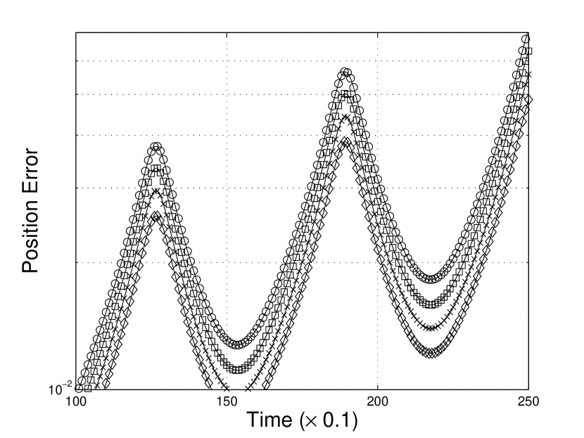
Figure 1: Figure 1.

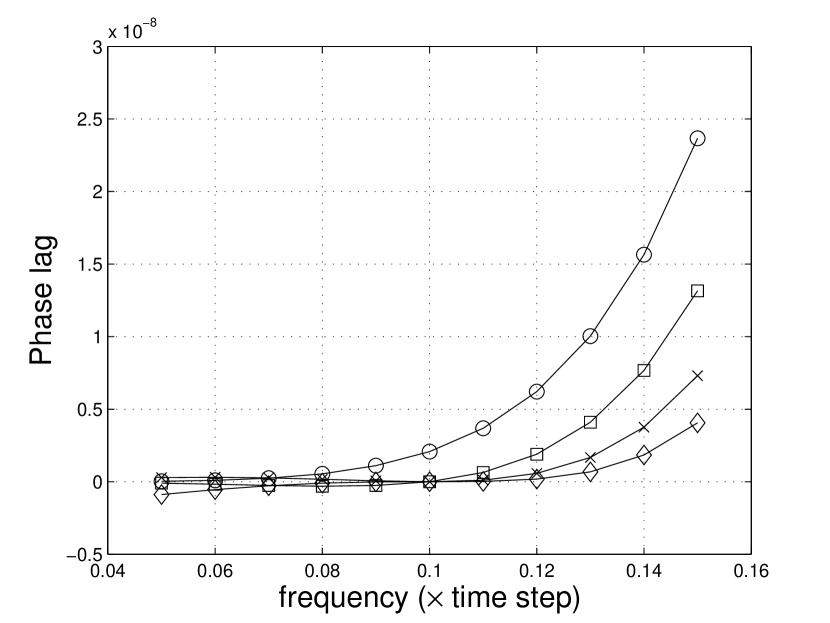
Figure 2: Figure 2.

References

- [1] Z.A. Anastassi and T.E. Simos. Special optimized runge-kutta methods for ivps with oscillating solutions. International Journal of Modern Physics C, 15:1–15, 2004.
- [2] Z.A. Anastassi and T.E. Simos. Trigonometrically fitted fifth order runge-kutta methods for the numerical solution of the schrödinger equation. Mathematical and Computer Modelling, 42:877–886, 2005.
- [3] Z.A. Anastassi and T.E. Simos. A trigonometrically-fitted runge-kutta method for the numerical solution of orbital problems. New Astronomy, 10:301–309, 2005.
- [4] Z.A. Anastassi and T.E. Simos. A family of exponentially-fitted runge-kutta methods with exponential order up to three for the numerical solution of the schrödinger equation. Journal of Mathematical Chemistry, 41:79–100, 2007.
- [5] G. Vanden Berghe and M. Van Daele. Exponentially-fitted stormer/ verlet methods. JNAIAM, 1(3):241–255, 2006.
- [6] L. Brusa and L. Nigro. A one-step method for direct integration of structural dynamic equations. Int. J. Num. Methods Engrg., 15:685–699, 1980.
- [7] J. R. Cash and F. Mazzia. Hybrid mesh selection algorithms based on conditioning for two-point boundary value problems. JNAIAM, 1(1):89–90, 2006.
- [8] M.M. Chawla and P.S. Rao. A numerov-type method with minimal phase-lag for the integration of second order periodic initial-value problems. ii. explicit method. J.Comput.Appl.Math., 15:329, 1986.
- [9] W. Gautschi. Numerical integration of ordinary differential equations based on trigonometric polynomials. Numer. Math., 3:381–397, 1961.
- [10] F. Iavernaro, F. Mazzia, and D. Trigiante. Stability and conditioning in numerical analysis. JNAIAM, 1(1):91–112, 2006.
- [11] L.Gr. Ixaru and G. Vanden Berghe. Exponential Fitting. Kluwer Academic Publishers, Dordrecht/Boston/London, 2004.
- [12] L.Gr. Ixaru and M. Rizea. A numerov-like scheme for the numerical solution of the schrödinger equation in the deep continuum spectrum of energies. Comp. Phys. Comm., 19:23–27, 1980.
- [13] J.D. Lambert and I.A. Watson. Symmetric multistep methods for periodic initial values problems. J. Inst. Math. Appl., 18:189–202, 1976.
- [14] T. Lyche. Chebyshevian multistep methods for ordinary differential equations. Num. Math., 19:65–75, 1972.
- [15] F. Mazzia, A. Sestini, and D. Trigiante. Bs linear multistep methods on non-uniform meshes. JNAIAM, 1(1):131–144, 2006.
- [16] G. Psihoyios. A block implicit advanced step-point (bias) algorithm for stiff differential systems. CoLe, 2(1-2):51–58, 2006.
- [17] D. Raptis and A.C. Allison. Exponential-fitting methods for the numerical solution of the schrödinger equation. Computer Physics Communications, 14:1, 1978.
- [18] T.E. Simos. A four-step method for the numerical solution of the schrödinger equation. J. Comput. Appl. Math., 30:251–255, 1990.
- [19] T.E. Simos. Some new four-step exponential-fitting methods for the numerical solution of the schrödinger equation. IMA J. Num. Anal., 11:347–356, 1991.
- [20] T.E. Simos. Error analysis of exponential-fitted methods for the numerical solution of the one-dimensional schrödinger equation. Phys. Lett. A, 177:345–350, 1993.
- [21] T.E. Simos. Specialist Periodical Reports. The Royal Society of Chemistry, Cambridge, 2000.
- [22] T.E. Simos. P-stable four-step exponentially-fitted method for the numerical integration of the schrödinger equation. CoLe, 1(1):37–45, 2005.
- [23] T.E. Simos. Closed newton-cotes trigonometrically-fitted formulae for numerical integration of the schrödinger equation. CoLe, 1(3):45–57, 2007.