Classical to quantum transition of a driven nonlinear nanomechanical resonator

Abstract

Much experimental effort is invested these days in fabricating nanoelectromechanical systems (NEMS) that are sufficiently small, cold, and clean, so as to approach quantum mechanical behavior as their typical quantum energy scale $\hbar\Omega$ becomes comparable to that of the ambient thermal energy $k_{B}T$. Such systems will hopefully enable one to observe the quantum behavior of human-made objects, and test some of the basic principles of quantum mechanics. Here we expand and elaborate on our recent suggestion [Phys. Rev. Lett. 99 (2007) 040404] to exploit the nonlinear nature of a nanoresonator in order to observe its transition into the quantum regime. We study this transition for an isolated resonator, as well as one that is coupled to a heat bath at either zero or finite temperature. We argue that by exploiting nonlinearities, quantum dynamics can be probed using technology that is almost within reach. Numerical solutions of the equations of motion display the first quantum corrections to classical dynamics that appear as the classical-to-quantum transition occurs. This provides practical signatures to look for in future experiments with NEMS resonators.

1 Motivation: Mechanical Systems at the Quantum Limit

This special focus issue of the New Journal of Physics is motivated by the growing interest in the study of “Mechanical Systems at the Quantum Limit”. Nanoelectromechanical systems (NEMS) [1, 2, 3, 4, 5] offer one of the most natural playgrounds for such a study [6, 7, 8]. With recent experiments coming within less than an order of magnitude from the ability to observe quantum zero-point motion [9, 10, 11], ideas about the quantum-to-classical transition (QCT) [12, 13, 14] may soon become experimentally accessible, more than 70 years after Schrödinger described his famous cat paradox [15]. As nanomechanical resonators become smaller, their masses decrease and natural frequencies $\Omega$ increase—exceeding 1GHz in recent experiments [16, 17]. For such frequencies it is sufficient to cool down to temperatures on the order of $50mK$ for the quantum energy $\hbar\Omega$ to be comparable to the thermal energy $k_{B}T$. Cooling well below such temperatures should allow one to observe truly quantum mechanical phenomena, such as resonances, oscillator number states, superpositions, and entanglement [18, 19, 20, 21, 22], at least for macroscopic objects that are sufficiently isolated from their environment.

Here we expand and elaborate on our recent suggestion [23] to exploit the nonlinear nature of NEMS resonators [24] in order to study the transition into the quantum domain. Nonlinear behavior of NEMS (and MEMS) resonators is frequently observed in experiments [1, 25, 26, 27, 28, 29, 30, 31, 32, 33], offers interesting theoretical challenges [34, 35, 36, 37], and can also be exploited for applications [38, 39, 40, 41]. Here we study a driven nonlinear nanomechanical resonator, also known as the Duffing resonator. We choose the system parameters such that the classical Duffing resonator is in a regime in which, in the presence of dissipation, it can oscillate at one of two different amplitudes, or one of two dynamical steady-states of motion, depending on its initial conditions. This dependence on initial conditions has recently been mapped-out by Kozinsky et al. [33] in an experiment with a nanoresonator. Thermally-induced switching between the two dynamical steady-states of motion has also been observed in a nanoresonator experiment by Aldridge and Cleland [30].

Naturally, the question arises whether quantum-mechanically the resonator can be driven into a superposition of the two possible steady-states of motion, or at least tunnel or switch between them at temperatures that are sufficiently low for thermal switching to be suppressed, but not necessarily so low to satisfy the constraint $k_{B}T\ll\hbar\Omega$ for observing full-fledged quantum mechanics. To answer this question we perform two separate calculations on the same Duffing resonator, viewing it once as a quantum-mechanical object and once as a classical object. With everything else being equal, this allows us to contrast the dynamics of a classical resonator with that of its quantum clone. We can then search for a regime in which quantum dynamics just begins to deviate away from classical dynamics, providing us with practical signatures that can be detected experimentally.

We calculate the dynamics numerically. We start each quantum calculation with a coherent state, which is a minimal wave-packet centered about some point in phase space. We start the corresponding classical calculation with an ensemble of initial conditions—typically of $N=10^{4}$ points—drawn from a Gaussian distribution in phase space that is identical to the initial quantum-mechanical probability density. We perform these calculations for three qualitatively different situations: An isolated resonator with no coupling to the environment; a resonator coupled to a heat bath at temperature $T_{env}=0$; and a resonator coupled to a heat bath at a finite temperature $T_{env}>0$. In all cases we display the calculated quantum dynamics in phase space using the quantum Wigner function

$$W(x,p,t)={\frac{1}{\pi\hbar}}\int_{\infty}^{\infty}dx^{\prime}e^{-{2i\over\hbar}px^{\prime}}\langle x+x^{\prime}|\rho(t)|x-x^{\prime}\rangle,$$ (1)

where $\rho(t)$ is the usual density operator, and compare it with the time-evolution of the classical phase-space density. We remind the reader that the Wigner function is not a true probability distribution as it may possess negative values, particularly when the quantum state has no classical analog. Nevertheless, it reduces to the quantum probability $P(x,t)$ of observing the system at position $x$ at time $t$ upon integration over $p$, and vice versa.

The paper is organized as follows. Section 2 gives a general discussion of the transition from quantum to classical dynamics, and the corresponding limit of $\hbar\to 0$. Section 3 describes the classical and quantum mechanical equations of motion for an isolated resonator, and section 4 discusses the results of our calculation for the isolated case. In Section 5 we describe the dynamics of a resonator that is coupled to a heat bath, and in Sections 6 and 7 we present the results of our calculation for a resonator, coupled to a zero-temperature and a finite-temperature bath respectively. We summarize and discuss the significance of our results in Section 8, concluding with some ideas for future directions.

2 The Quantum to Classical Transition (QCT)

Everyday macroscopic objects behave according to classical physics, expressed in terms of Newton’s or Hamilton’s equations of motion. Since these objects are composed of atoms and molecules, one expects this classical behavior to emerge from quantum dynamics under a certain limit of high temperature, large masses, and high energies, all characterizing the macroscopic world. It is commonly accepted that the transition between the quantum and the classical descriptions occurs by letting $\hbar$ go to zero. Of course $\hbar$ is actually a non-zero physical constant with the dimensionality of action, so whenever one says that “$\hbar$ goes to zero” one actually means that some dimensionless combination of $\hbar$ with a physical quantity characterizing the system—like its ratio to the classical action $\hbar/S$—goes to zero.

One can see in a number of different ways that classical dynamics should be obtained from the quantum description by letting $\hbar\rightarrow 0$. If one expresses the quantum mechanical wave function as $\psi=\sqrt{\rho}\exp[iS/\hbar]$, then upon letting $\hbar\rightarrow 0$ the Schrödinger equation reduces to the classical Hamilton-Jacoby equation for $S$ [45, Section 6.4]. The Feynman path integral approach to quantum mechanics, in which one sums over all paths between two points in space and time, reduces to Hamilton’s principle of classical mechanics, identifying the classical path for which the action satisfies $\delta S=0$ [46]. Finally, one can look at the equation of motion for the quantum Wigner function (1). This equation can be obtained using the von Neumann equation for the density operator $\rho(t)$,

$$\dot{\rho}=\frac{1}{i\hbar}[H_{sys},\rho],$$ (2)

where $H_{sys}$ is the Hamiltonian of the system. For a general potential $U(x)$, which can be expanded in a Taylor series, one gets the quantum Liouville equation [47],

$$\left(\partial_{t}+\frac{p}{m}\partial_{x}-\frac{dU(x)}{dx}\partial_{p}\right)W(x,p,t)=\sum_{n=1}^{\infty}\frac{(-1)^{n}(\hbar/2)^{2n}}{(2n+1)!}\partial_{x}^{2n+1}U(x)\partial_{p}^{2n+1}W(x,p,t).$$ (3)

If one formally sets $\hbar=0$, and unless the derivatives of the Wigner function on the right-hand side become singular, the right-hand side is equal to zero and one recovers the classical Liouville equation for the distribution in phase space.

It turns out that this naive approach does not work in general, and that one often encounters non-analyticities in quantum mechanics as one takes the limit $\hbar\rightarrow 0$ [48]. For an isolated system, the classical Liouville and master equations (see Section 3) violate unitarity, as well as the quantum restriction of the density matrix to be semi-positive definite. Thus, the limit $\hbar\rightarrow 0$ cannot be connected smoothly to $\hbar=0$. Therefore, as long as the dynamics considered is of an isolated system, the evolution of a quantum observable will in general agree with the corresponding classical average only up to a finite time, called the Ehrenfest time, $t_{E}$. For non chaotic systems, it is expected that $t_{E}$ will have some power law dependence on $\hbar$, $t_{E}\sim\hbar^{-\delta}$, though the exact value of $\delta$ may depend on the model [51, 52, 53]. Nevertheless, we observe here that it is difficult strictly to define the time scale at which a separation between classical and quantum dynamics occurs, mainly because this time scale seems to depend on the observable one chooses to measure. Generally, it seems that there is no single time scale, as described by Oliveira et al. [54, 55].

The contemporary approach to understanding the classical limit of quantum mechanics—stemming from early work of Feynman and Vernon [56] and Caldeira and Leggett [57]—is to look at a more realistic model, in which the system of interest is coupled in some way to the external world, generically referred to as ‘an environment’, whether it is another system or a measuring device [42, 43, 58]. The interaction with the environment must be taken into account, and one distinguishes between two types of systems, depending on whether a measurement is performed on the environment or not [59, 60, 61]. If the environment is not observed, then the appropriate description of the system is in terms of the reduced density operator, obtained by tracing the full density matrix over the variables of the environment. Time evolution is then given by a master equation, and the so called weak form of QCT is obtained by comparing quantum and classical distributions. This is what we do here, while noting in agreement with Habib et al. [52] that the role of the environment is actually two-fold. On one hand, it destroys interference patterns with negative values in the Wigner function that are incompatible with a classical probability density. On the other hand, it causes the classical fine structure to smear over a thermal scale, producing a classical distribution without the infinitely-small fine structure, which is incompatible with quantum mechanics owing to the finite value of $\hbar$ and the uncertainty principle.

If the environment is measured, the reduced density matrix depends on the outcome of the measurements, and the evolution is said to be conditioned on the observation results, as described for example by Habib et al. [61]. This type of evolution can yield effectively classical trajectories, and is called the strong form of QCT. We shall analyze the latter case, which requires more advanced tools of quantum measurement theory, in a future publication.

3 Isolated System – Method of Calculation

We consider a nonlinear resonator, such as a doubly-clamped nanomechanical beam [31, 32], nanowire [62, 63], or nanotube [64, 65], vibrating in its fundamental flexural mode, and thus treated as a single degree of freedom. The resonator is driven, in any of the standard NEMS techniques [4, 5], by an external periodic force and is either isolated from its environment—a case treated in this section—or coupled to the environment in the form of a heat bath at a temperature $T_{env}$—a case that will be treated later. The Hamiltonian for such a driven nonlinear resonator, known as the Duffing resonator, is

$$\tilde{H}_{sys}=\frac{1}{2m}\tilde{p}^{2}+\frac{m\Omega^{2}}{2}\tilde{x}^{2}+\frac{\varepsilon}{4}\tilde{x}^{4}-\tilde{x}\tilde{F}\cos\tilde{\omega}\tilde{t},$$ (4)

where $m$ is the effective mass of the resonator, $\Omega$ its normal frequency, $\varepsilon$ the strength of nonlinearity, $\tilde{F}$ the driving amplitude, and $\tilde{\omega}$ the driving frequency. Throughout the discussion here, and with no loss of generality, we consider the case of a stiffening nonlinearity, with $\varepsilon>0$.

We change from the physical variables, denoted by tildes, to dimensionless variables without tildes, by measuring time in units of $1/\Omega$, mass in units of $m$, and length in units of $\sqrt{m\Omega^{2}/\varepsilon}$. The dimensionless Hamiltonian $H_{sys}$ is then measured in units of the characteristic energy $m^{2}\Omega^{4}/\varepsilon$,

$$H_{sys}=\frac{1}{2}p^{2}+\frac{1}{2}x^{2}+\frac{1}{4}x^{4}-xF\cos\omega t,$$ (5)

where $x$, $p$, and $t$ are now measured in the dimensionless units, and $F=\tilde{F}\sqrt{\varepsilon}(m\Omega^{2})^{-\frac{3}{2}}$ and $\omega=\tilde{\omega}/\Omega$ are the dimensionless driving amplitude and frequency, respectively. The degree to which we approach the quantum domain is indicated by an increasing effective value of $\hbar$ as compared with a measure of the classical action $S$ of the system, both stated in terms of the scaled units $m^{2}\Omega^{3}/\varepsilon$. For the case of transverse vibrations of a doubly-clamped beam, as shown by Lifshitz and Cross [24], the nonlinear coefficient $\varepsilon$ is given by $m\Omega^{2}/d^{2}$ to within a numeral factor of order unity, where $d$ is the width, or diameter, of the beam. Thus, the scaled units of action become $m\Omega d^{2}$. We shall reinterpret these values later in terms of real experimental masses, frequencies, and widths.

3.1 Classical dynamics – Hamilton and Liouville equations

Hamilton’s equations give the equations of motion for $x$ and $p$,

$$\dot{x} = p$$ (6)

$$\dot{p} = -x-x^{3}+F\cos\omega t.$$ (7)

For the isolated resonator, the classical Liouville equation for the phase-space distribution function $f(x,p,t)$ is

$$\frac{\partial f}{\partial t}=-\{f,H_{sys}\},$$ (8)

where $\{\cdot,\cdot\}$ denotes the Poisson brackets. Upon substituting the Hamiltonian (4) one gets (denoting $\partial_{x}\equiv{\partial}/{\partial x}$ etc.)

$$\partial_{t}f=-\left[p\partial_{x}+\left(-x-x^{3}+F\cos\omega t\right)\partial_{p}\right]f,$$ (9)

where $x$ and $p$ are treated as independent variables. The initial state $f(x,p,t=0)$ is taken to be a Gaussian distribution centered at some $[x_{0},p_{0}]$ and having standard deviations of $\Delta x=\sqrt{\hbar/2}$ and $\Delta p=\sqrt{\hbar/2}$, corresponding to an initial quantum coherent state with minimum uncertainty $\Delta x\Delta p=\hbar/2$.

We can examine the case of a linear resonator simply by omitting the cubic term in (7). In this case the result is a set of linear ODE’s that can be solved analytically. For the nonlinear case we integrate the equation of motion (7) numerically. The solution enables us to calculate ensemble averages and make plots of the density in phase space. Instead of keeping track of all the trajectories as a function of time, we calculate a histogram of the probability density $f(x,p,t)$. We do so by dividing phase space using a grid, where each entry of the grid counts the number of trajectories passing through a particular square in phase space at any given time. This grid is then used to calculate the classical averages. The discrete nature of the grid and the finite number of initial conditions (typically 10⁴) is the reason for the apparent differences between the initial classical and quantum states shown in the Figures below.

3.2 Quantum dynamics – The Schrödinger equation

The quantum Hamiltonian operator of the driven Duffing resonator is the same as (4),

$$H_{sys}=\hbar\left(a^{\dagger}a+\frac{1}{2}\right)+\frac{\hbar^{2}}{16}\left(a^{\dagger}+a\right)^{4}-\sqrt{\frac{\hbar}{2}}\left(a^{\dagger}+a\right)F\cos\omega t,$$ (10)

where we have used the ordinary definition of the ladder operators

$$a = \frac{1}{\sqrt{2\hbar}}(x+ip),$$ (11a)

$$a^{{\dagger}} = \frac{1}{\sqrt{2\hbar}}(x-ip).$$ (11b)

We simply solve the corresponding Schrödinger equation numerically by advancing the wave function in discrete time steps $\Delta t$, using the interaction-picture time-evolution operator. We do so by expanding the wave function in a truncated energy basis $|n\rangle$, with $n\leq N$. The value of $N$, which is typically $\approx 50$, is determined by the requirement that the high-energy basis states are never significantly occupied. We use the wave function at time $t$ to calculate and then plot the corresponding Wigner function.

4 Isolated System – Results

All results in this section are given for a choice of parameters $F=0.01$ and $\omega=1.018$, which ensures that the resonator is in the bistability region. The results are shown in Figure 1 by plotting the Wigner function next to the sampled classical phase-space density, for the initial minimal Gaussian wave packet and its later evolution at three different times, measured in periods of the drive $T=2\pi/\omega$. We note that the apparent discreteness of the classical distributions, as opposed to the smooth quantum Wigner functions, stems from the fact that the former are generated from a histogram on a discrete grid. The densities are raised to the power $1/4$ for better color contrast, where blue denotes positive values, and red denotes negative values. A square of area $\hbar$ is shown at the bottom right corner of the initial state plot to indicate the scale of $\hbar$.

We see that for short times the positive (blue) outline of the Wigner function resembles that of the classical distribution (Figure 1b). In addition, a strong interference pattern is evident within this outline. In all the snapshots it is evident that the Wigner function has a strong positive density where the classical density is also large. Nevertheless, two differences between the quantum and classical distributions are evident, namely, the strong interference pattern which exists in the Wigner function even in the steady state, and the infinitely fine structure which develops in the classical distribution. These differences demonstrate that taking the limit of $\hbar\to 0$ does not give rise to the emergence of classical dynamics from the quantum description, as indicated earlier in Section 2.

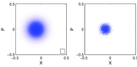
(a) Initial coherent state, $t=0$

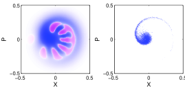
(b) $t=30T$

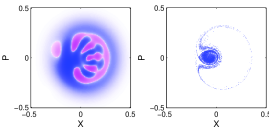
(c) $t=156T$

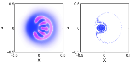
(d) $t=300T$

Figure 1: Isolated Duffing resonator with $\hbar=0.008$. Wigner function (left) and classical distribution (right) of the initial minimal Gaussian wave packet and its evolution at three later times, measured in terms of the drive period $T=2\pi/\omega$. A square of area $\hbar$ is shown at the bottom right corner of the initial state plot. The functions are scaled by $f\rightarrow f^{1/4}$ for better color contrast.

We can, however, use the approach proposed by Berry [48], where the quantum probability density is averaged over $x$ and $p$ to account for the limited precision of a typical measuring device. If we do the same here, and replace the value of the Wigner function $W(x,p)$ with its averaged value over a small area of size $\delta x\delta p$ around the point $(x,p)$, the negative and positive parts of the interference pattern cancel each other out. If we perform the same averaging also for the classical distribution, the classical fine structure is smeared, bringing the two distributions even closer in appearance, as shown in Figure 2.

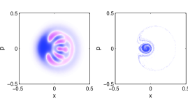
(a) Original distributions

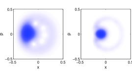
(b) Averaged distributions

Figure 2: Isolated Duffing resonator with $\hbar=0.008$. (a) Original Wigner function and classical distribution (left and right, respectively), shown after 300 periods of the drive, as obtained from the calculations shown in Fig. 1. (b) The same distributions averaged using a Gaussian kernel of area $2\hbar$. The functions are scaled to the power of $1/2$.

We use the calculated phase-space densities in order to try to estimate the time scale $t_{E}$ at which the quantum and classical correspondence is broken. We do so by measuring the distance in phase space between the quantum and classical expectation values of the first and second moments of $x$ and $p$ as a function of time, scaled by the distance of the classical phase-space point from the origin. This measure,

$$\Delta^{n}=\frac{\sqrt{(\langle x^{n}\rangle-x_{cl}^{n})^{2}+(\langle p^{n}\rangle-p_{cl}^{n})^{2}}}{\sqrt{(x_{cl}^{n})^{2}+(p_{cl}^{n})^{2}}},\qquad n=1,2,$$ (11l)

gives us the relative divergence of the quantum expectation values from the classical ones, where $\langle\cdot\rangle$ denotes the quantum expectation value, and the subscript ${cl}$ denotes the classical ensemble average. The results for $\Delta^{1}$ and $\Delta^{2}$ are shown in Fig. 3 on a semi-log scale as a function of time, along with their values averaged over one period of the drive. For both values of the effective $\hbar$ that are shown it appears difficult to determine the Ehrenfest times $t_{E}$. Even if one insists on making such a determination, it seems to depend on the power of $x$ and $p$ being measured, and the resulting estimates are inconclusive. Therefore, we cannot determine the Eherenfest times in our model with any real certainty.

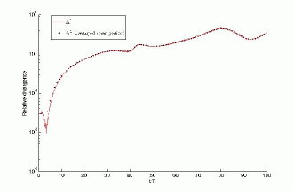
(a) $n=1,\hbar=0.032$

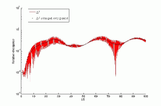
(b) $n=2,\hbar=0.032$

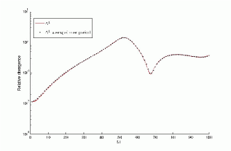
(c) $n=1,\hbar=0.008$

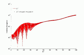
(d) $n=2,\hbar=0.008$

Figure 3: Relative divergence of quantum and classical expectation values for the isolated driven Duffing resonator, calculated using Eq. (11l). One cannot conclusively estimate the Ehrenfest times $t_{E}$ for the cases examined here.

5 Open System – Method of Calculation

We now couple the Duffing resonator to an external environment by introducing a thermal bath. As usual, this coupling introduces dissipation due to loss of energy from the resonator to the bath, as well as fluctuations due to the random forces applied by the heat bath to the resonator. We use different approaches to add this coupling to either the classical or quantum-mechanical resonators, as outlined below.

5.1 Open classical dynamics – Langevin equation

In the classical calculation, dissipation is introduced using a Langevin approach, adding two terms to the equation of motion for $p$. The first is a velocity dependent friction force $-\gamma\dot{x}$, and the second is a time dependent random force $\delta F(t)$ acting on the resonator. Note that these additional terms are dimensionless and measured using the units that were introduced earlier. In particular, $\gamma$ is in fact the inverse of the dimensionless quality factor $Q$. The random force is assumed to be a $\delta$-correlated Gaussian white noise, satisfying

$$\langle\delta F(t)\rangle=0,$$ (11m)

$$\langle\delta F(t)\delta F(t^{\prime})\rangle=2\gamma k_{B}T_{env}\delta(t-t^{\prime}),$$ (11n)

where $k_{B}$ is Boltzman’s constant, thus introducing the bath temperature $T_{env}$. The equations of motion become

$$\dot{x} = p,$$ (11oa)

$$\dot{p} = -x-x^{3}-\gamma p+F\cos\omega t+\delta F(t),$$ (11ob)

and are integrated numerically, as in the case of the isolated system.

5.2 Open quantum dynamics – Master equation

To describe the evolution of a quantum Duffing resonator that is coupled to an environment we can proceed either by using a quantum Langevin approach [42], or by coupling the resonator to a bath of harmonic resonators [42, 66]. The latter approach, which we follow here, adds two terms to the Hamiltonian (10)—a Hamiltonian for the bath and an interaction Hamiltonian—resulting in

$$\ H_{tot}=H_{sys}+H_{bath}+V.$$ (11op)

The von Neumann equation (2) for the total density operator $\rho_{tot}$, describing the resonator and the bath, is

$$\dot{\rho}_{tot}=\frac{1}{i\hbar}[H_{tot},\rho_{tot}],$$ (11oq)

where the resonator alone is now described by the reduced density operator, obtained by tracing out the bath degrees of freedom,

$$\rho_{sys}(t)=Tr_{bath}\left\{\rho_{tot}(t)\right\}.$$ (11or)

We use a standard interaction Hamiltonian [21] of the Caldeira-Leggett [57] type in the rotating-wave approximation,

$$V=\sum_{i}(\kappa_{i}b_{i}a^{\dagger}+\kappa_{i}^{*}b_{i}^{\dagger}a),$$ (11os)

where the $\kappa_{i}$ are bilinear coupling constants, the $b_{i}$ are annihilation operators acting on the bath oscillators, and $a$ is the annihilation operator of the Duffing resonator (11a and $b$). Note that a different choice of coupling other than Eq. (11os) may lead to a different Master equation.

By assuming the interaction to be weak, and by employing the Markov approximation which assumes that the bath has no memory, we obtain a standard master equation [21, 42, 66],

$$\dot{\rho}_{sys} = \frac{1}{i\hbar}[H_{sys},\rho_{sys}]-\frac{\gamma}{2}(1+\bar{n})(a^{\dagger}a\rho_{sys}+\rho_{sys}a^{\dagger}a-2a\rho_{sys}a^{\dagger})$$ (11ot)

$$- \frac{\gamma}{2}\bar{n}(aa^{\dagger}\rho_{sys}+\rho_{sys}aa^{\dagger}-2a^{\dagger}\rho_{sys}a),$$

where $\bar{n}\equiv(e^{\hbar\Omega/k_{B}T_{env}}-1)^{-1}$ is the Bose-Einstein distribution through which $T_{env}$ is introduced, $\gamma\equiv 2\pi g(\Omega)|\kappa(\Omega)|^{2}$ is interpreted as the damping rate, $g(\Omega)$ is the density of states of the bath, evaluated at the resonator’s natural frequency, and $\kappa(\Omega)$ is the coupling constant at the resonator’s natural frequency. We evaluate these two variables at the natural frequency $\Omega=1$, because the shift in the resonator’s frequency due to nonlinearity is assumed small.

The resulting master equation (11ot) is of a Lindblad form [42, 58, 67], which in the Schrödinger picture is given by

$$\dot{\rho}=\frac{1}{i\hbar}[\tilde{H},\rho]-\frac{1}{2}\sum_{m}(C_{m}^{\dagger}C_{m}\rho+\rho C_{m}^{\dagger}C_{m})+\sum_{m}C_{m}\rho C_{m}^{\dagger},$$ (11ou)

where $\tilde{H}$ may differ from $H_{sys}$, for example due to a Lamb shift of the resonator’s natural frequency. The non-unique operators $C_{m}$ and $C_{m}^{\dagger}$ operate on the Hilbert space of the resonator. Identifying the Lindblad form enables us to avoid solving the master equation directly—a solution which demands extensive computation. Instead, we use the Monte-Carlo wave function method (MCWF) [59, 68], which is computationally more efficient. It is based on computing many time evolutions of the initial quantum state, so-called quantum trajectories, with a non-hermitian Hamiltonian that implements the stochastic action of the bath and is derived from $H_{sys}$. Subsequent averaging over the different trajectories yields the correct time evolution of the density operator that satisfies the master equation (11ot). We carry out the MCWF numerically using MATLAB.

6 Open System at $T_{env}=0$ – Results

We begin by considering the coupling of the driven Duffing resonator to a zero-temperature bath. Again, we choose the values of the different parameters $F=0.015$, $\omega=1.018$, and $\gamma=0.01$, such that the driven nonlinear resonator is operating in its bistability regime. For $T_{env}=0$, in the quantum dynamics the average phonon number $\bar{n}=0$, and in the classical dynamics we expect to see damping without the smearing effect of a random force. Thus, the ability of the environment to induce transitions between the dynamic states of the resonator is suppressed. We look at a value of $\hbar=0.004$, as shown in Fig. 4, where the initial state is placed within the basin of attraction of the large amplitude classical stable solution. The Gaussian classical phase-space distribution all flows, as expected, to a single point—the fixed point corresponding to the large-amplitude dynamical state.

In the quantum dynamics, at short times we again see a general positive outline of the Wigner function which is similar to the classical density, as for the isolated Duffing resonator in Section 4, but it quickly deviates from the classical distribution. The uncertainly principle prevents it from shrinking to a point as in the classical dynamics. More importantly, we clearly observe that the Wigner distribution has substantial weight around the state of small-amplitude oscillations, which is inaccessible classically for the chosen initial conditions at $T_{env}=0$. The quantum resonator can still switch between the two stable dynamical states, even though the classical resonator cannot. This switching takes place either via tunneling—in analogy with the macroscopic quantum tunneling between two equilibrium states of a static system [19]—or via quantum activation [69, 70], although at this point it is impossible for us to distinguish between these two processes.

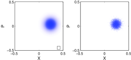
(a) Initial coherent state, $t=0$

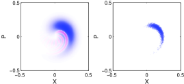
(b) $t=10T$

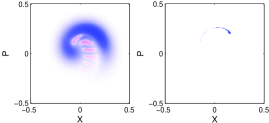
(c) $t=80T$

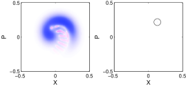
(d) $t=300T$

Figure 4: A driven Duffing resonator coupled to a zero-temperature heat bath with scaled $\hbar=0.004$ (other parameters are listed in the text). Wigner functions (left) and classical phase-space distributions (right) of the initial minimal Gaussian wave packet—located within the basin of attraction of the large-amplitude dynamical state—and its evolution at three later times. The large-amplitude fixed point, towards which the classical distribution flows, is encircled in Figure (d). A square of area $\hbar$ is shown at the bottom right corner of the initial state plot. The functions are scaled by $f\rightarrow f^{1/4}$ for a better color contrast.

7 Open System at $T_{env}>0$ – Results

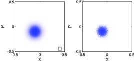
(a) Initial coherent state, $t=0$

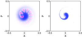
(b) $t=30T$

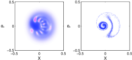
(c) $t=180T$

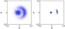
(d) $t=800T$

Figure 5: The driven Duffing resonator coupled to a heat bath at $k_{B}T_{env}=2\hbar\Omega$ with $\hbar=0.004$. Wigner function (left) and classical distribution (right) of an initial minimal Gaussian wave packet—straddling the separatrix between the regions in phase space flowing to the two stable states—and its evolution at three later times. A square of area $\hbar$ is shown at the bottom right corner of the initial state plot. The functions are scaled by $f\rightarrow f^{1/4}$ for a better color contrast.

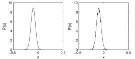
(a) Initial coherent state, $t=0$

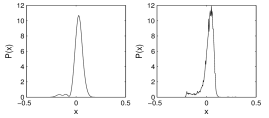
(b) $t=30T$

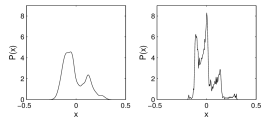
(c) $t=180T$

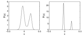
(d) $t=800T$

Figure 6: Probability densities $P(x)$ for the same four states shown in Fig. 5, obtained by integrating the phase-space distributions in the $p$ direction. The $y$ axis is scaled differently for better visualization.

Figure 5 shows the calculated results for a Duffing resonator with $\hbar=0.004$, coupled to a heat bath at a finite temperature $k_{B}T_{env}=2\hbar\Omega$. This temperature is obtained by adding a fluctuating force according to the fluctuation-dissipation relation (11n). To avoid having a random force whose magnitude dominates the dynamics we reduce the damping rate to $\gamma=0.001$, thus requiring a longer time for the resonator to reach its final steady state. The remaining parameters are chosen to be $F=0.006$ and $\omega=1.016$ to ensure that the resonator is still operating in the bistability regime.

Here we choose the initial Gaussian state to straddle the separatrix between regions in phase space that flow to the two stable states. The interference pattern that develops for short times within the general positive outline in the Wigner function is soon destroyed by decoherence, and becomes jittery in space and time. At long times, both distributions peak around the two stable states, nevertheless they differ significantly. The classical density is tightly localized around the two solutions with no overlap, indicating that $T_{env}$ is too small to induce thermal switching of the classical resonator between the two states, as was observed in a recent experiment [30]. The Wigner function, on the other hand, is spread out in phase space, indicating that $\hbar$ is sufficiently large for the quantum resonator to switch between the two states via tunneling or quantum activation [69, 70]. This is demonstrated more clearly in Fig. 6, which shows the probability distributions $P(x)$, that are obtained by integrating the phase-space distributions in Fig. 5 in the $p$ direction.

Further analysis shows that only for temperatures as high as $k_{B}T=17\hbar\Omega$ does the classical phase-space distribution become as wide as the Wigner function is at $k_{B}T=2\hbar\Omega$, as demonstrated in Fig. 7. Thus, in a real experiment, evidence for quantum-mechanical dynamics can be demonstrated as long as temperature and other sources of noise can be controlled to better than an order of magnitude. Note also that minor differences exist between the high-temperature classical distribution and the low-temperature quantum distribution (e.g. the relative heights of the two peaks in the probability density $P(x)$, as seen in Fig. 7(b)), which may assist in distinguishing between the two possibilities.

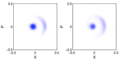
(a)  Phase space densities, $t=800T$

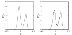
(b)  Probability densities of $x$, $t=800T$

Figure 7: As in Figs. 5(d) and  6(d), only that the classical calculation (right) is for $k_{B}T_{env}=17\hbar\Omega$, yielding (a) similar phase-space distributions; and (b) similar probability densities. Both distributions in (a) are left unscaled.

As we lower the temperature, for example, down to $k_{B}T_{env}=\hbar\Omega$, we see further deviations of the quantum dynamics from the classical one. Figure 8 shows the unscaled Wigner functions of the state at $t=800T$ for the two temperatures. In both cases the function is almost all positive with small negative parts, and are peaked around the two classical stable solutions. Nevertheless, one sees that the similarity to the classical distribution is evidently higher for the higher temperature.

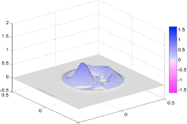
(a) $k_{B}T_{env}=\hbar\Omega$

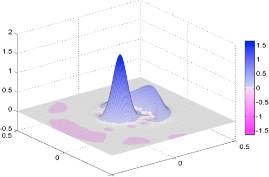
(b) $k_{B}T_{env}=2\hbar\Omega$

Figure 8: The driven Duffing resonator coupled to a heat bath at $k_{B}T_{env}=\hbar\Omega$ and at $k_{B}T_{env}=2\hbar\Omega$ with $\hbar=0.004$. Unscaled Wigner functions of the state at $t=800T$ are plotted for the two temperatures. As in Fig. 5, the initial Gaussian state straddles the separatrix so that the classical distribution splits towards both of the two stable dynamical states. With the decrease in temperature one sees further deviation away from classical behavior.

8 Discussion

We have calculated the classical evolution and the quantum evolution of a driven Duffing resonator, whether isolated or coupled to an environment. For the case of an isolated resonator—which is less relevant for experiment, yet still interesting theoretically—we have confirmed that the quantum and classical evolutions are essentially different, and that the transition from one picture to the other does not take place in a simple manner. The non-analytic nature of the limit $\hbar\to 0$ appears in the form of strong quantum interference patterns in the Wigner function, describing the quantum evolution, which are never suppressed in the absence of coupling to an environment. In addition, one observes an infinitely fine structure in the classical phase-space distribution, which is absent from the quantum distribution, owing to the uncertainty principle that smears any structure on the scale of $\hbar$. We have shown that these differences can be resolved by introducing a constraint on the experimental resolution. An uncertainty in the measurement on the order of $\hbar$ can both smear the fine structure in the classical distribution and average out the interference pattern in the quantum Wigner function, giving rise to similarly-looking phase-space distributions, as demonstrated in Fig. 2.

In all cases investigated here—whether for an isolated resonator or one that is coupled to an environment—we have found that at very early stages of the evolution the quantum Wigner function and the classical phase-space distribution agree with each other. As can be seen in Figs. 1(b), 4(b), and 5(b), at early times the Wigner function contains a positive backbone which closely resembles the classical distribution, even though a quantum interference pattern develops within this backbone. One expects that up to some Ehrenfest time there will be a corresponding agreement between quantum observables and classical averages. Nevertheless, even though such agreement is observed we could not consistently and conclusively estimate the Ehrenfest time.

Only after coupling the driven Duffing resonator to an environment at temperature $T_{env}$ was it possible to search for the regime of interest that we set out to find at the beginning of this work. We wanted to find a regime that would enable us to observe the first deviations away from classical behavior as we pass through the so-called classical-to-quantum transition. We have found this regime by gradually decreasing the physical dimensions of the system, or equivalently by increasing the effective value of $\hbar$, as measured by the physical scale $m\Omega d^{2}$, set by the parameters of the system. We have found an appropriate set of parameters—$\hbar\approx 10^{-3}$, $k_{B}T_{env}=2\hbar\Omega$, and $Q\approx 10^{3}$ with a corresponding forcing amplitude that puts the Duffing resonator in its bistable regime—for which the quantum dynamics, as it appears in the Wigner function, looks very much like classical dynamics, but at the same time shows clear signatures that it is not classical.

We should ask how far we are from reaching such parameters in realistic systems with current technology. Reaching quality factors on the order of hundreds to thousands is quite routine with standard suspended elastic beam resonators and somewhat optimistic with suspended nanotubes, while exciting these resonators into their nonlinear regime and observing hysteresis due to bistability is very common. Reaching the required effective $\hbar\approx 10^{-3}$ implies that one needs $m\Omega d^{2}\approx 10^{-31}$ m²kg/s. For a NEMS beam [31, 32] with $d\approx 10$nm and $m\approx 10^{-18}$kg, vibrating at $\Omega\approx 10^{8}$Hz, we obtain $m\Omega d^{2}\approx 10^{-26}$ m²kg/s, which is 5 orders of magnitude too large. On the other hand, with suspended nanowires [62, 63] or nanotubes [64, 65] with $d\approx 1$nm and $m\approx 10^{-21}$kg, also vibrating at $\Omega\approx 10^{8}$Hz, we obtain $m\Omega d^{2}\approx 10^{-31}$ m²kg/s, which is exactly what we want. Note that 100MHz is quite a high natural frequency for a nanotube. For a lower frequency, one would obtain an even better value for the effective $\hbar$, but this would require working at extremely low temperatures, while for $\Omega\approx 100$MHz we would need $T_{env}\approx 10$mK. Thus, we believe that with slight improvement over current technology, one would be able to see the classical-to-quantum transition described here, by taking advantage of the nonlinear nature of doubly-clamped nanoresonators.

Clearly, the most striking signature of quantum dynamics is the appearance of quantum interference with negative regions in the Wigner function. It would be wonderful if, at some point in the future, one could directly measure the Wigner function and observe these negative regions, as one can already do, for example, in the case of trapped atoms [71]. Before such direct measurement is possible, we suggest to perform experiments along the lines of the weak from of QCT that we have studied here. In such experiments one should prepare the system in a particular initial point $(x,p)$ in phase space, let it evolve, and observe it at some later time $t$. Repeating the same experiment 10,000 times, will allow one to generate a histogram of measured positions $x(t)$, similar to the numerical histograms shown in Fig. 6. We emphasize that in this kind of experimental protocol, the quantum state of the system—assuming it is indeed quantum—is destroyed in the measurement process, a time $t$ after it is initialized, but otherwise one is free of any considerations of quantum measurement theory.

It is possible to recognize clear signatures while performing such an experiment, implying that a driven Duffing resonator, working in its bistability regime, is behaving in accordance with the laws of quantum mechanics. In both cases one should operate in a regime of $\hbar$ and $T_{env}$ similar to the one used here, in which thermal switching between the two dynamical steady-states of the resonator is exponentially suppressed, whereas quantum switching is possible. Under such circumstances one can look for the following signatures:

1. If the initial coherent state is prepared within the basin of attraction of one of the two steady-state solutions of the dynamical system, as we did in section 6, the classical ensemble should flow as a whole to this solution at long times, while parts of the quantum Wigner function should flow to the other steady-state solution. This yields a finite probability of finding the quantum resonator oscillating in a dynamical state that is inaccessible for the classical resonator.

2. Even if the initial coherent state straddles over both basins of attraction, as we showed in section 7, and both distributions split between the two steady-state solutions, at long times there is a nonzero probability of finding the quantum resonator in a position between the two steady-state solutions, while classically this probability is zero.

An interesting question that we have not yet addressed here, is whether the quantum switching that we see takes place via tunneling or quantum activation, as suggested by Marthaler and Dykman [69, 70]. We will address this question in a future publication where we will consider individual quantum trajectories of our system, possibly while performing a continuous weak measurement, along the lines of the strong form of QCT.

References

References

- [1] H.G. Craighead. Nanoelectromechanical systems. Science, 290:1532, 2000.
- [2] M.L. Roukes. Plenty of room indeed. Scientific American, 285:42, 2001.
- [3] M.L. Roukes. Nanoelectromechanical systems face the future. Physics World, 14:25, 2001.
- [4] A.N. Cleland. Foundations of Nanomechanics. Springer, Berlin, 2003.
- [5] K. L. Ekinci and M. L. Roukes. Nanoelectromechanical systems. Review of Scientific Instruments, 76:061101, 2005.
- [6] A. Cho. Researchers race to put the quantum into mechanics. Science, 299:36–37, 2003.
- [7] M. P. Blencowe. Quantum electromechanical systems. Physics Reports, 395:159–222, 2004.
- [8] K.C. Schwab and M.L. Roukes. Putting mechanics into quantum mechanics. Physics Today, 58:36–42, July 2005.
- [9] R.G. Knobel and A.N. Cleland. Nanometre-scale displacement sensing using a single electron transistor. Nature, 424:291, 2003.
- [10] M. D. LaHaye, O. Buu, B. Camarota, and K. C. Schwab. Approaching the quantum limit of a nanomechanical resonator. Science, 304(5667):74–77, 2004.
- [11] A. Naik, O. Buu, M. D. LaHaye, A. D. Armour, A. A. Clerk, M. P. Blencowe, and K. C. Schwab. Cooling a nanomechanical resonator with quantum back-action. Nature, 443(7108):193–196, 2006.
- [12] Roger Penrose. On gravity‘s role in quantum state reduction. Gen. Relativ. Gravit., 28:581–600, 1996.
- [13] A. J. Leggett. The significance of the MQC experiment. J. Supercond., 12(6):683–687, 1999.
- [14] A. J. Leggett. Testing the limits of quantum mechanics: motivation, state of play, prospects. J. Phys.: Cond. Mat., 14(15):R415–R451, 2002.
- [15] E. Schrödinger. Naturwissenschaften, 23:807, 1935.
- [16] X. M. H. Huang, C. A. Zorman, M. Mehregany, and M. L. Roukes. Nanodevice motion at microwave frequencies. Nature, 421:496, 2003.
- [17] A. N. Cleland and M. R. Geller. Superconducting qubit storage and entanglement with nanomechanical resonators. Phys. Rev. Lett., 93:070501, 2004.
- [18] V. Peano and M. Thorwart. Macroscopic quantum effects in a strongly driven nanomechanical resonator. Physical Review B (Condensed Matter and Materials Physics), 70(23):235401, 2004.
- [19] S. M. Carr, W. E. Lawrence, and M. N. Wybourne. Accessibility of quantum effects in mesomechanical systems. Phys. Rev. B, 64:220101(R), 2001.
- [20] A. D. Armour, M. P. Blencowe, and K. C. Schwab. Entanglement and decoherence of a micromechanical resonator via coupling to a cooper-pair box. Phys. Rev. Lett., 88:148301, 2002.
- [21] D. H. Santamore, A. C. Doherty, and M. C. Cross. Quantum nondemolition measurement of fock states of mesoscopic mechanical oscillators. Phys. Rev. B, 70:144301, 2004.
- [22] J. Eisert, M. B. Plenio, S. Bose, and J. Hartley. Towards quantum entanglement in nanoelectromechanical devices. Phys. Rev. Lett., 93:190402, 2004.
- [23] I. Katz, A. Retzker, R. Straub, and R. Lifshitz. Signatures for a classical to quantum transition of a driven nonlinear nanomechanical resonator. Phys. Rev. Lett., 99(4):040404, 2007.
- [24] Ron Lifshitz and M. C. Cross. Nonlinear dynamics of nanomechanical and micromechanical resonators, volume 1 of Review of Nonlinear Dynamics and Complexity, chapter 1. Wiley, Berlin, 2008.
- [25] K. L. Turner, S. A. Miller, P. G. Hartwell, N. C. MacDonald, S. H. Strogatz, and S. G. Adams. Five parametric resonances in a microelectromechanical system. Nature, 396:149–152, 1998.
- [26] E. Buks and M.L̃. Roukes. Metastability and the casimir effect in micromechanical systems. Europhys. Lett., 54:220, 2000.
- [27] E. Buks and M. L. Roukes. Electrically tunable collective response in a coupled micromechanical array. J. MEMS, 11:802–807, 2002.
- [28] D.V. Scheible, A. Erbe, and R.H. Blick. Evidence of a nanomechanical resonator being driven into chaotic response via the Ruelle-Takens route. Appl. Phys. Lett., 81:1884, 2002.
- [29] M. Yu, G. J. Wagner, R. S. Ruoff, and M. J. Dyer. Realization of parametric resonances in a nanowire mechanical system with nanomanipulation inside a scanning electron microscope. Phys. Rev. B, 66:073406, 2002.
- [30] J. S. Aldridge and A. N. Cleland. Noise-enabled precision measurements of a duffing nanomechanical resonator. Phys. Rev. Lett., 94(15):156403, 2005.
- [31] H.W.Ch. Postma, I. Kozinsky, A. Husain, and M.L. Roukes. Dynamic range of nanotube- and nanowire-based electromechanical systems. Appl. Phys. Lett., 86:223105, May 2005.
- [32] I. Kozinsky, H.W.Ch. Postma, I. Bargatin, and M.L. Roukes. Tuning nonlinearity, dynamic range, and frequency of nanomechanical resonators. Appl. Phys. Lett., 88:253101, Jun 2006.
- [33] I. Kozinsky, H. W. Ch. Postma, O. Kogan, A. Husain, and M. L. Roukes. Basins of attraction of a nonlinear nanomechanical resonator. Phys. Rev. Lett., 99:207201, 2007.
- [34] Ron Lifshitz and M. C. Cross. Response of parametrically driven nonlinear coupled oscillators with application to micromechanical and nanomechanical resonator arrays. Phys. Rev. B, 67(13):134302, 2003.
- [35] Yaron Bromberg, M. C. Cross, and Ron Lifshitz. Response of discrete nonlinear systems with many degrees of freedom. Phys. Rev. E, 73(1):016214, 2006.
- [36] M. C. Cross, A. Zumdieck, Ron Lifshitz, and J. L. Rogers. Synchronization by nonlinear frequency pulling. Phys. Rev. Lett., 93:224101, 2004.
- [37] M. C. Cross, J. L. Rogers, Ron Lifshitz, and A. Zumdieck. Synchronization by reactive coupling and nonlinear frequency pulling. Phys. Rev. E, 73(3):036205, 2006.
- [38] D. Rugar and P. Grütter. Mechanical parametric amplification and thermomechanical noise squeezing. Phys. Rev. Lett., 67(6):699–702, Aug 1991.
- [39] D. W. Carr, S. Evoy, L. Sekaric, H. G. Craighead, and J. M. Parpia. Parametric amplification in a torsional microresonator. Appl. Phys. Lett., 77:1545–1547, 2000.
- [40] A. Lupascu, E.F.C. Driessen, L. Roschier, C.J.P.M. Harmans, and J.E. Mooij. High-contrast dispersive readout of a superconducting flux qubit using a nonlinear resonator. Phys. Rev. Lett., 96(12):127003, 2006.
- [41] M.J. Woolley, A.C. Doherty, G.J. Milburn, and K.C. Schwab. Nanomechanical squeezing with detection via a microwave cavity. eprint arXiv:quant-ph/0803.1757v1, 2008.
- [42] C.W. Gardiner and P. Zoller. Quantum Noise. Springer, Berlin, 3rd edition, 2004.
- [43] D.F. Walls and G.J. Milburn. Quantum Optics. Springer, Berlin, 1994.
- [44] A. Sergi and F. Petruccione. Nosé-Hoover dynamics in quantum phase space. eprint arXiv:quant-ph/0711.2207v1, 2007.
- [45] Louis N. Hand and Janet D. Finch. Analytical Mechanics. Cambridge University Press, Cambridge, 1998.
- [46] R. P. Feynman and A. R. Hibbs. Quantum Mechanics and Path Integrals. McGraw-Hill, 1965.
- [47] W.P. Schleich. Quantum Optics in Phase Space. Wiley-VCH, Berlin, 2001.
- [48] M. V. Berry. Some Quantum-to-Classical Asymptotics, volume LII of Les Houches Lecture Series, Eds. M.J. Giannoni and A. Voros and J. Zinn-Justin, chapter 4. Elsevier, 1991.
- [49] S. Habib, K. Jacobs, H. Mabuchi, R. Ryne, K. Shizume, and B. Sundaram. Quantum-classical transition in nonlinear dynamical systems. Phys. Rev. Lett., 88(4):040402, Jan 2002.
- [50] Omri Gat. Quantum dynamics and breakdown of classical realism in nonlinear oscillators. J. Phys. A: Math. Theor., 40:F911–F920, 2007.
- [51] M. V. Berry and N. L. Balazs. Evolution of semiclassical quantumm states in phase space. J. Phys. A: Math. Gen., 12(5):625–642, 1978.
- [52] S. Habib, K. Shizume, and W. H. Zurek. Decoherence, chaos, and the correspondence principle. Phys. Rev. Lett., 80(20):4361–4365, May 1998.
- [53] F. Cametti and C. Presilla. Quantum breaking time near classical equilibrium points. Phys. Rev. Lett., 89(4):040403, 2002.
- [54] A. C. Oliveira, M. C. Nemes, and K. M. F. Romero. Quantum time scales and the classical limit: Analytic results for some simple systems. Phys. Rev. E, 68:036214, 2003.
- [55] A. C. Oliveira, J. G. Peixoto de Faria, and M. C. Nemes. Quantum-classical transition of the open quartic oscillator: The role of the environment. Phys. Rev. E, 73:046207, 2006.
- [56] R. P. Feynman and F. L. Vernon. The theory of a general quantum system interacting with a linear dissipative system. Ann. Phys., 24:118–173, 1963.
- [57] A.O. Caldeira and A.J. Leggett. Quantum tunnelling in a dissipative system. Ann. Phys., 149(2):374–456, september 1983.
- [58] Maximilian Schlosshauer. Decoherence and the quantum to classical transition. Springer, Berlin, 2007.
- [59] M.B. Plenio and P.L. Knight. The quantum-jump approach to dissipative dynamics in quantum optics. Rev. Mod. Phys., 70(1):101–144, Jan 1998.
- [60] B. D. Greenbaum, S. Habib, K. Shizume, and B. Sundaram. The semiclassical regime of the chaotic quantum-classical transition. Chaos, 15(3):033302, 2005.
- [61] S. Habib, T. Bhattacharya, A. Doherty, B. Greenbaum, A. Hopkins, K. Jacobs, H. Mabuchi, K. Schwab, K. Shizume, D. Steck, and B. Sundaram. Nonlinear quantum dynamics. eprint arXiv:quant-ph/0505046, 2005.
- [62] A. Husain, J. Hone, Henk W. Ch. Postma, X. M. H. Huang, T. Drake, M. Barbic, A. Scherer, and M. L. Roukes. Nanowire-based very-high-frequency electromechanical resonator. Appl. Phys. Lett., 83(6):1240–1242, 2003.
- [63] X.L. Feng, R.R. He, P.D. Yang, and M.L. Roukes. Very high frequency silicon nanowire electromechanical resonators. Nano Lett., 7:1953–1959, Jul 2007.
- [64] V. Sazonova, Y. Yaish, H. Üstünel, D. Roundy, T.A. Arias, and P.L. McEuan. A tunable carbon nanotube electromechanical oscillator. Nature, 431:284–287, Sep 2004.
- [65] B. Witkamp, M. Poot, and H.S.J. van der Zant. Bending-mode vibration of a suspended nanotube resonator. Nano Lett., 6:2904 – 2908, Dec 2006.
- [66] W. Louisell. Quantum Statistical Properties of Radiation. Wiley, New York, 1973.
- [67] H. Spohn. Kinetic equations from hamiltonian dynamics. Rev. Mod. Phys., 52:569–615, 1980.
- [68] K. Mølmer, Y. Castin, and J. Dalibard. Monte carlo wave-function method in quantum optics. J. Opt. Soc. Am. B, 10:524, 1993.
- [69] M. Marthaler and M. I. Dykman. Switching via quantum activation: A parametrically modulated oscillator. Phys. Rev. A, 73:042108, 2006.
- [70] M. I. Dykman. Critical exponents in metastable decay via quantum activation. Phys. Rev. E, 75:011101, 2007.
- [71] D. Leibfried, D.M. Meekhof, B.E. King, C. Monroe, W.M. Itano, and D.J. Wineland. Experimental determination of the motional quantum state of a trapped atom. Phys. Rev. Lett., 77(21):4281–4285, Nov 1996.