The pattern of genetic hitchhiking under recurrent mutation

Abstract

Genetic hitchhiking describes evolution at a neutral locus that is linked to a selected locus. If a beneficial allele rises to fixation at the selected locus, a characteristic polymorphism pattern (so-called selective sweep) emerges at the neutral locus. The classical model assumes that fixation of the beneficial allele occurs from a single copy of this allele that arises by mutation. However, recent theory (Pennings and Hermisson, 2006a, b) has shown that recurrent beneficial mutation at biologically realistic rates can lead to markedly different polymorphism patterns, so-called soft selective sweeps. We extend an approach that has recently been developed for the classical hitchhiking model (Schweinsberg and Durrett, 2005; Etheridge et al., 2006) to study the recurrent mutation scenario. We show that the genealogy at the neutral locus can be approximated (to leading orders in the selection strength) by a marked Yule process with immigration. Using this formalism, we derive an improved analytical approximation for the expected heterozygosity at the neutral locus at the time of fixation of the beneficial allele.

1 Introduction

The model of genetic hitchhiking, introduced by Maynard Smith and Haigh (1974), describes the process of fixation of a new mutation due to its selective advantage. During this fixation process, linked neutral DNA variants that are initially associated with the selected allele will hitchhike and also increase in frequency. As a consequence, sequence diversity in the neighborhood of the selected locus is much reduced when the beneficial allele fixes, a phenomenon known as a selective sweep. This characteristic pattern in DNA sequence data can be used to detect genes that have been adaptive targets in the recent evolutionary history by statistical tests (e.g. Kim and Stephan 2002; Nielsen et al. 2005; Jensen et al. 2007).

Since its introduction, several analytic approximations to quantify the hitchhiking effect have been developed (Kaplan et al., 1989; Stephan et al., 1992; Barton, 1998; Schweinsberg and Durrett, 2005; Etheridge et al., 2006; Eriksson et al., 2008). The mathematical analysis of selective sweeps makes use of the coalescent framework (Kingman, 1982; Hudson, 1983), which describes the genealogy of a population sample backward in time. Most studies follow the suggestion of Kaplan et al. (1989) and use a structured coalescent to describe the genetic footprint at a linked neutral locus, conditioned on an approximated frequency path of the selected allele. In this approach, population structure at the neutral locus consists of the wild-type and beneficial background at the selected locus, respectively. A mathematical rigorous construction was given by Barton et al. (2004). Moreover, a structured ancestral recombination graph was used in Pfaffelhuber and Studeny (2007); McVean (2007); Pfaffelhuber et al. (2008) to describe the common ancestry of two neutral loci linked to the beneficial allele.

It has long been noted that the initial rise in frequency of a beneficial allele is similar to the evolution of the total mass of a supercritical branching process (Fisher 1930; Kaplan et al. 1989; Barton 1998; Ewens 2004, p. 27f). This insight led to the approximation of the structured coalescent by the genealogy of a supercritical branching process—a Yule process (O’Connell, 1993; Evans and O’Connell, 1994). Given a selection intensity of $\alpha$ and a recombination rate of $\rho$ between the selected and neutral locus, it has been shown that a Yule process with branching rate $\alpha$, which is marked at rate $\rho$ and stopped upon reaching $\lfloor 2\alpha\rfloor$ lines, is an accurate approximation of the structured coalescent (Schweinsberg and Durrett, 2005; Etheridge et al., 2006; Pfaffelhuber et al., 2006). For the standard scenario of genetic hitchhiking, this approach leads to a refined analytical approximation of the sampling distribution, estimates of the approximation error and to efficient numerical simulations.

The classical hitchhiking model assumes that adaptation occurs from a single origin of the beneficial allele. An explicit mutational process at the selected locus, where the beneficial allele can enter the population recurrently, is not taken into account. However, it has recently been demonstrated that recurrent beneficial mutation at a biologically realistic rate can lead to considerable changes in the selective footprint in DNA sequence data (Hermisson and Pennings, 2005; Pennings and Hermisson, 2006a, b). In the present paper, we extend the Yule process approach of Etheridge et al. (2006) to the full biological model with recurrent mutation at the beneficial locus. Specifically, we show that the genealogy at the selected site can be approximated by a Yule process with immigration. Our results can serve as a basis for a detailed analysis of patterns of genetic hitchhiking under recurrent mutation, such as the site-frequency spectrum and linkage disequilibrium patterns. As an example of such an application, we derive the expected heterozygosity in Section 3.3.

The paper is organized as follows. In Section 2, we introduce the model as well as the structured coalescent and we discuss the biological context of our work. In Section 3 we state results on the adaptive process, give the approximation of the structured coalescent by a Yule process with immigration and apply the approximation to derive expressions for the heterozygosity at the neutral locus at the time of fixation. In Sections 4, 5 and 6 we collect all proofs.

2 The model

We describe evolution in a two-locus system, where a neutral locus is linked to a locus experiencing positive selection. In Section 2.1, we first focus on the selected locus and formulate the adaptive process as a diffusion. In Section 2.2, we describe the genealogy at the neutral locus by a structured coalescent. In Section 2.3 we discuss the biological context.

2.1 Time-forward process

Consider a population of constant size $N$. Individuals are haploid; their genotype is thus characterized by a single copy of each allele. Selection acts on a single bi-allelic locus. The ancestral (wild-type) allele $b$ has fitness $1$ and the beneficial variant $B$ has fitness $1+s$, where $s>0$ is the selection coefficient. Mutation from $b$ to $B$ is recurrent and occurs with probability $u$ per individual per generation. Let $X_{t}$ be the frequency of the $B$ allele in generation $t$. In a standard Wright-Fisher model with discrete generations, the number of $B$-alleles in the offspring generation $t+1$ is $NX_{t+1}$, which is binomially distributed with parameters $\frac{(1+s)X_{t}+u(1-X_{t})}{(1+s)X_{t}+1-X_{t}}$ and $N$.

We assume that the beneficial allele $B$ is initially absent from the population in generation $t=0$ when the selection pressure on the $B$ locus sets in. Since the $B$ allele is created recurrently by mutation and we ignore back-mutations it will eventually fix at some time $T$, i.e. $X_{t}=1$ for $t\geq T$. This process of fixation can be approximated by a diffusion. To this end, let $\mathcal{X}^{N}=(X_{t}^{N})_{t=0,1,2,\ldots}$ with $X^{N}_{0}=0$ be the path of allele frequencies of $B$.

Assuming $u=u_{N}\to 0,s=s_{N}\to 0$ such that $2Nu\to\theta,Ns\to\alpha$ as $N\to\infty$, it is well-known (see e.g. Ewens 2004) that $(X^{N}_{\lfloor 2Nt\rfloor})_{t\geq 0}\Rightarrow(X_{t})_{t\geq 0}$ as $N\to\infty$ where $\mathcal{X}:=(X_{t})_{t\geq 0}$ follows the SDE

$$dX =\big{(}\tfrac{\theta}{2}(1-X)+\alpha X(1-X)\big{)}dt+\sqrt{X(1-X)}dW$$ (2.1)

with $X_{0}=0$. In other words, the diffusion approximation of $\mathcal{X}^{N}$ is given by a diffusion $\mathcal{X}$ with drift and diffusion coefficients

$$\mu_{\alpha,\theta}(x)=(\tfrac{\theta}{2}+\alpha x)(1-x),\qquad\sigma^{2}(x)=x(1-x).$$

We denote by $\mathbb{P}^{p}_{\alpha,\theta}[.]$ and $\mathbb{E}^{p}_{\alpha,\theta}[.]$ the probability distribution and its expectation with respect to the diffusion with parameters $\mu_{\alpha,\theta}$ and $\sigma^{2}$ and $X_{0}=p$ almost surely. The fixation time can be expressed in the diffusion setting as

$$T:=\inf\{t\geq 0:X_{t}=1\}.$$ (2.2)

2.2 Genealogies

We are interested in the change of polymorphism patterns at a neutral locus that is linked to a selected locus. We ignore recombination within the selected and the neutral locus, but (with sexual reproduction) there is the chance of recombination between the selected and the neutral locus. Let the recombination rate per individual be $\rho$ in the diffusion scaling (i.e. $r=r_{N}$ is the recombination probability in a Wright-Fisher model of size $N$ and $r_{N}\xrightarrow{N\to\infty}0$ and $Nr_{N}\xrightarrow{N\to\infty}\rho$). Not all recombination events have the same effect, however. We will be particularly interested in events that change the genetic background of the neutral locus at the selected site from $B$ to $b$, or vice-versa. This is only possible if $B$ individuals from the parent generation reproduce with $b$ individuals. Under the assumption of random mating, the effective recombination rate in generation $t$ that changes the genetic background is thus $\rho X_{t}(1-X_{t})$ in the diffusion setting.

Following Barton et al. (2004), we use the structured coalescent to describe the polymorphism pattern at the neutral locus in a sample. In this framework, the population is partitioned into two demes according to the allele ($B$ or $b$) at the selected locus. The relative size of these demes is defined by the fixation path $\mathcal{X}$ of the $B$ allele. Only lineages in the same deme can coalesce. Transition among demes is possible by either recombination or mutation at the selected locus. We focus on the pattern at the time $T$ of fixation of the beneficial allele. Throughout we fix a sample size $n$.

Remark 2.1.

We define the coalescent as a process that takes values in partitions and introduce the following notation. Denote by $\Sigma_{n}$ the set of partitions of $\{1,...,n\}$. Each $\xi\in\Sigma_{n}$ is thus a set $\xi=\{\xi_{1},...,\xi_{|\xi|}\}$ such that $\bigcup_{i=1}^{|\xi|}\xi_{i}=\{1,...,n\}$ and $\xi_{i}\cap\xi_{j}=\emptyset$ for $i\neq j$. Partitions can also be defined by equivalence relations and we write $k\sim_{\xi}\ell$ iff there is $1\leq i\leq|\xi|$ such that $k,\ell\in\xi_{i}$. Equivalently, $\xi$ defines a map $\xi:\{1,...,n\}\to\{1,...,|\xi|\}$ by setting $\xi(k)=i$ iff $k\in\xi_{i}$. We will also need the notion of a composition of two partitions. If $\xi$ is a partition of $\{1,...,n\}$ and $\eta$ is a partition of $\{1,...,|\xi|\}$, define the partition $\xi\circ\eta$ on $\{1,...,n\}$ by $k\sim_{\xi\circ\eta}\ell$ iff $\xi(k)\sim_{\eta}\xi(\ell)$.∎

Setting $\beta=T-t$ we are interested in the genealogical process $\xi^{\mathcal{X}}=(\xi_{\beta})_{0\leq\beta\leq T}$ of a sample of size $n$, conditioned on the path $\mathcal{X}$ of the beneficial allele $B$. The state space of $\xi^{\mathcal{X}}$ is

$$S_{n}:=\{(\xi^{B},\xi^{b}):\xi^{B}\cup\xi^{b}\in\Sigma_{n}\}.$$

Elements of $\xi^{B}$ ($\xi^{b}$) are ancestral lines of neutral loci that are linked to a beneficial (wild-type) allele. Since there are only beneficial alleles at time $T$, the starting configuration of $\xi^{\mathcal{X}}$ is

$$\xi^{\mathcal{X}}_{0}=(\{1\},...,\{n\},\emptyset).$$

For a given coalescent state $\xi^{\mathcal{X}}_{\beta}=(\xi^{B},\xi^{b})$ at time $\beta$, several events can occur, with rates that depend on the value of the frequency path $\mathcal{X}$ at that time, ${X}_{T-\beta}$. Coalescences of pairs of lines in the beneficial (wild-type) background occur at rate $1/X_{T-\beta}$ ($1/(1-X_{T-\beta})$). Formally, for all pairs $1\leq i<j\leq|\xi^{B}|$ and $1\leq i^{\prime}<j^{\prime}\leq|\xi^{b}|$, transitions occur at time $\beta$ to

$$\big{(}(\xi^{B}\setminus\{\xi^{B}_{i},\xi^{B}_{j}\})\cup\{\xi^{B}_{i}\cup\xi^{B}_{j}\},\xi^{b}\big{)} \qquad\text{ with rate }\qquad\frac{1}{X_{T-\beta}}$$ (2.3)

$$\big{(}\xi^{B},(\xi^{b}\setminus\{\xi^{b}_{i^{\prime}},\xi^{b}_{j^{\prime}}\})\cup\{\xi^{b}_{i^{\prime}}\cup\xi^{b}_{j^{\prime}}\}\big{)} \qquad\text{ with rate }\qquad\frac{1}{1-X_{T-\beta}}.$$

Changes of the genetic background happen either due to mutation at the selected locus or recombination events between the selected and the neutral locus. For $1\leq i\leq|\xi^{B}|$, transitions of genetic backgrounds due to mutation occur at time $\beta$ from $\xi^{\mathcal{X}}_{\beta}=(\xi^{B},\xi^{b})$ for $1\leq i\leq|\xi^{B}|$ to

$$\big{(}\xi^{B}\setminus\{\xi^{B}_{i}\},\xi^{b}\cup\{\xi^{B}_{i}\}\big{)} \qquad\text{ with rate }\qquad\frac{\theta}{2}\frac{1-X_{T-\beta}}{X_{T-\beta}}.$$ (2.4)

(Recall that we assume that there are no back-mutations to the wild-type). Moreover, changes of the genetic background due to recombination occur at time $\beta$ for $1\leq i\leq|\xi^{B}|$, $1\leq i^{\prime}\leq|\xi^{b}|$ from $\xi^{\mathcal{X}}_{\beta}=(\xi^{B},\xi^{b})$ to

$$\big{(}\xi^{B}\setminus\{\xi^{B}_{i}\},\xi^{b}\cup\{\xi^{B}_{i}\}\big{)} \qquad\text{ with rate }\qquad\rho(1-X_{T-\beta})$$ (2.5a)

$$\big{(}\xi^{B}\cup\{\xi^{b}_{i^{\prime}}\},\xi^{b}\setminus\{\xi^{b}_{i^{\prime}}\}\big{)} \qquad\text{ with rate }\qquad\rho X_{T-\beta}.$$ (2.5b)

All rates of $\xi^{\mathcal{X}}$ are collected in Table 1.

event	coal in $B$	coal in $b$	mut from $B$ to $b$	rec from $B$ to $b$	rec from $b$ to $B$
rate	$\frac{1}{X_{t}}$	$\frac{1}{1-X_{t}}$	$\frac{\theta}{2}\frac{1-X_{t}}{X_{t}}$	$\rho(1-X_{t})$	$\rho X_{t}$

Table 1: Transition rates in the process $\xi^{\mathcal{X}}$ at time $t=T-\beta$. Coalescence rates are equal for all pairs of partition elements in the beneficial and wild-type background. Recombination and mutation rates are equal for all partition elements in $\xi^{B}$ and $\xi^{b}$.

Remark 2.2.

1. The rates for mutation and recombination can be understood heuristically. Assume $X_{t}^{N}=x$ and assume $u,s,r$ are small. A neutral locus linked to a beneficial allele in generation $t+1$ falls into one of three classes: (i) the class for which the ancestor of the selected allele was beneficial has frequency $x+\mathcal{O}(u,s,r)$; (ii) the class for which the beneficial allele was a wild-type and mutated in the last generation has frequency $u(1-x)+\mathcal{O}(us,ur)$; (iii) the class for which the neutral locus was linked to a wild-type allele in generation $t$ and recombined with a beneficial allele has frequency $rx(1-x)+\mathcal{O}(ru,rs)$). Hence, if we are given a neutral locus in the beneficial background, the probability that its linked selected locus experienced a mutation one generation ago is $\frac{u(1-x)}{x}+\mathcal{O}(u^{2},us,ur)$ and that it recombined with a wild-type allele one generation ago is $\frac{rx(1-x)}{x}+\mathcal{O}(ru,rs,r^{2})$. Thus, the rates (2.4) and (2.5a) arise by a rescaling of time by $N$.

2. In (2.3) and (2.4) the rates have singularities when $X_{T-\beta}=0$. However, we will show in Lemma 5.3 using arguments from Barton et al. (2004) and Taylor (2007) that a line will almost surely leave the beneficial background before such a singularity occurs. In particular, the structured coalescent process $\xi^{\mathcal{X}}$ is well-defined.

2.3 Biological context

A selective sweep refers to the reduction of sequence diversity and a characteristic polymorphism pattern around a positively selected allele. Models show that this pattern is most pronounced close to the selected locus if selection is strong and if the sample is taken in a short time window after the fixation of the beneficial allele (i.e. before it is diluted by new mutations). Today, biologists try to detect sweep patterns in genome-wide polymorphism scans in order to identify recent adaptation events (e.g. Harr et al., 2002; Ometto et al., 2005; Williamson et al., 2005).

The detection of sweep regions is complicated by the fact that certain demographic events in the history of the population (in particular bottlenecks) can lead to very similar patterns. Vice-versa, also the footprint of selection can take various guises. In particular, recent theory shows that the pattern can change significantly if the beneficial allele at the time of fixation traces back to more than a single origin at the start of the selective phase (i.e. there is more than a single ancestor at this time). As a consequence, genetic variation that is linked to any of the successful origins of the beneficial allele will survive the selective phase in proximity of the selective target and the reduction in diversity (measured e.g. by the number of segregating sites or the average heterozygosity in a sample) is less severe. Pennings and Hermisson (2006a) therefore called the resulting pattern a soft selective sweep in distinction of the classical hard sweep from only a single origin. Nevertheless, also a soft sweep has highly characteristic features, such as a more pronounced pattern of linkage disequilibrium as compared to a hard sweep (Pennings and Hermisson, 2006b).

Soft sweeps can arise in several biological scenarios. For example, multiple copies of the beneficial allele can already segregate in the population at the start of the selective phase (adaptation from standing genetic variation; Hermisson and Pennings 2005; Przeworski et al. 2005). Most naturally, however, the mutational process at the selected locus itself may lead to a recurrent introduction of the beneficial allele. Any model, like the one in this article, that includes an explicit treatment of the mutational process will therefore necessarily also allow for soft selective sweeps. For biological applications the most important question then is: When are soft sweeps from recurrent mutation likely? The results of Pennings and Hermisson (2006a) as well as Theorem 1 in the present paper show that the probability of soft selective sweeps is mainly dependent on the population-wide mutation rate $\theta$. The classical results of a hard sweep are reproduced in the limit $\theta\to 0$ and generally hold as a good approximation for $\theta<0.01$ in samples of moderate size. For larger $\theta$, approaching unity, soft sweep phenomena become important.

Since $\theta$ scales like the product of the (effective) population size and the mutation rate per allele, soft sweeps become likely if either of these factors is large. Very large population sizes are primarily found for insects and microbial organisms. Consequently, soft sweep patterns have been found, e.g., in Drosophila (Schlenke and Begun, 2004) and in the malaria parasite Plasmodium falsiparum (Nair et al., 2007). Since point mutation rates (mutation rates per DNA base per generation per individual) are typically very small ($\sim 10^{-8}$), large mutation rates are usually found in situations where many possible mutations produce the same (i.e. physiologically equivalent) allele. This holds, in particular, for adaptive loss-of-function mutations, where many mutations can destroy the function of a gene. An example is the loss of pigmentation in Drosophila santomea (Jeong et al., 2008). But also adaptations in regulatory regions often have large mutation rates and can occur recurrently. A well-known example is the evolution of adult lactose tolerance in humans, where several mutational origins have been identified (Tishkoff et al., 2007).

Several extensions of the model introduced in Section 2 are possible. In a full model, we should allow for the possibility of back-mutations from the beneficial to the wild-type allele in natural populations. However, such events are rarely seen in any sample because such back-mutants have lower fitness and are therefore less likely to contribute any offspring to the population at the time of fixation. Another step towards a more realistic modeling of genetic hitchhiking under recurrent mutation would be to allow for beneficial mutation to the same (physiological) allele at multiple different positions of the genome. In such a model, recombination between the different positions of the beneficial mutation in the genome would complicate our analysis.

3 Results

The process of fixation of the beneficial allele is described by the diffusion (2.1). In Section 3.1, we will derive approximations for the fixation time $T$ of this process. These results will be needed in Section 3.2, where we construct an approximation for the structured coalescent $\xi^{\mathcal{X}}$.

3.1 Fixation times

In the study of the diffusion (2.1) the time $T$ of fixation of the beneficial allele (see (2.2)) is of particular interest. We decompose the interval $[0;T]$ by the last time a frequency of $X_{t}=0$ was reached, i.e., we define

$$T_{0} :=\sup\{t\geq 0:X_{t}=0\},\qquad T^{\ast}:=T-T_{0}.$$

Note that for $\theta\geq 1$, the boundary $x=0$ is inaccessible, such that $T_{0}=0,T^{\ast}=T$, almost surely, in this case.

Proposition 3.1.

1. Let $\gamma_{e}\approx 0.57$ be Euler’s $\gamma$. For $\theta>0$,

   $$\mathbb{E}^{0}_{\alpha,\theta}[T] =\frac{1}{\alpha}\Big{(}2\log(2\alpha)+2\gamma_{e}+\frac{1}{\theta}-\theta\sum_{n=1}^{\infty}\frac{1}{n(n+\theta)}\Big{)}+\mathcal{O}\Big{(}\frac{\log\alpha}{\alpha^{2}}\Big{)}+\frac{1}{\theta}\mathcal{O}\big{(}\alpha e^{-\alpha}\big{)}$$ (3.1)

2. For $\theta\geq 1$, almost surely, $T=T^{\ast}$.

3. For $0\leq\theta\leq 1$,

   $$\mathbb{E}^{0}_{\alpha,\theta}[T^{\ast}] =\frac{2}{\alpha}\big{(}\log(2\alpha)+\gamma_{e}\big{)}+\mathcal{O}\Big{(}\frac{\log\alpha}{\alpha^{2}}\Big{)}$$ (3.2)

4. For $\theta\geq 0$,

   $$\mathbb{V}^{0}_{\alpha,\theta}[T^{\ast}] =\mathcal{O}\Big{(}\frac{1}{\alpha^{2}}\Big{)}.$$ (3.3)

All error terms are in the limit for large $\alpha$ and are uniform on compacta in $\theta$.

Remark 3.2.

1. Note that (3.1) reduces to (3.2) for $\theta=1$ as it should since $T_{0}\xrightarrow{\theta\uparrow 1}0$.

2. For $\theta\leq 1$, we find that $\mathbb{E}^{0}_{\alpha,\theta}[T^{\ast}]$ is independent of $\theta$ to the order considered. In particular it is identical to the conditioned fixation time without recurrent mutation ($\theta=0$) that was previously derived (van Herwaarden and van der Wal, 2002; Hermisson and Pennings, 2005; Etheridge et al., 2006). A detailed numerical analysis (not shown) demonstrates that the passage times of the beneficial allele decrease at intermediate and high frequencies, but increase at low frequencies $X\lesssim 1/\alpha$ where recurrent mutation prevents the allele from dying out. Both effects do not affect the leading order and precisely cancel in the second order for large $\alpha$.

3. To leading order in $1/\theta$ and $\alpha$, the total fixation time (3.1) is

   $$\mathbb{E}^{0}_{\alpha,\theta}[T]\approx\frac{1}{\alpha\theta}+E^{0}_{\alpha,\theta}[T^{\ast}].$$

   Since the fixation probability of a new beneficial mutation is $P_{\text{fix}}\approx 2s$ and the rate of new beneficial mutations per time unit (of $N$ generations) is $N\theta/2$, mutations that are destined for fixation enter the population at rate $sN\theta=\alpha\theta$. The total fixation time thus approximately decomposes into the conditioned fixation time $\mathbb{E}[T^{\ast}]$ and the exponential waiting time for the establishment of the beneficial allele $\frac{1}{\alpha\theta}$.

4. In applications, selective sweeps are found with $\alpha\geq 100$. We can then ignore the error term $\tfrac{1}{\theta}\mathcal{O}\big{(}\alpha e^{-\alpha/2}\big{)}$ in (3.1) even for extremely rare mutations with $\theta\sim 10^{-10}$.

5. The proof of Proposition 3.1 can be found in Section 4.

3.2 The Yule approximation

We will provide a useful approximation of the coalescent process with rates defined in (2.3)–(2.5). As already seen in the last section the process of fixation of the beneficial allele can be decomposed into two parts. First, the beneficial allele has to be established, i.e., its frequency must not hit 0 any more. Second, the established allele must fix in the population. The first phase has an expected length of about $1/(\alpha\theta)$ and hence may be long even for large values of $\alpha$, depending on $\theta$. The second phase has an expected length of order $(\log\alpha)/\alpha$ and is thus short for large $\alpha$, independently of $\theta$. For the potentially long first phase we give an approximation for the distribution of the coalescent on path space by a finite Kingman coalescent. For the short second phase, we obtain an approximation of the distribution of the coalescent (which is started at time $T$) at time $T_{0}$ using a Yule process with immigration (which constructs a genealogy forward in time). To formulate our results, define

$$\beta_{0}:=T-T_{0}.$$

Setting $X_{t}=0$ for $t<0$ we will obtain approximations for the distribution of coalescent states at time $\beta_{0}$,

$$\xi_{\beta_{0}}:=(\xi_{\beta_{0}}^{B},\xi_{\beta_{0}}^{b}):=\int\mathbb{P}_{\alpha,\theta}[d\mathcal{X}]\xi_{\beta_{0}}^{\mathcal{X}},$$

and of the genealogies for $\beta>\beta_{0}$, i.e. in the phase prior to establishment of the beneficial allele,

$$\xi_{\geq\beta_{0}}:=(\xi_{\geq\beta_{0}}^{B},\xi_{\geq\beta_{0}}^{b}):=\int\mathbb{P}_{\alpha,\theta}[d\mathcal{X}](\xi_{\beta_{0}+t}^{\mathcal{X}})_{t\geq 0}.$$

Note that $\xi_{\beta_{0}}\in\mathbb{S}_{n}$ while $\xi_{\geq\beta_{0}}\in\mathcal{D}([0;\infty),\mathbb{S}_{n})$, the space of cadlag paths on $[0;\infty)$ with values in $\mathbb{S}_{n}$.

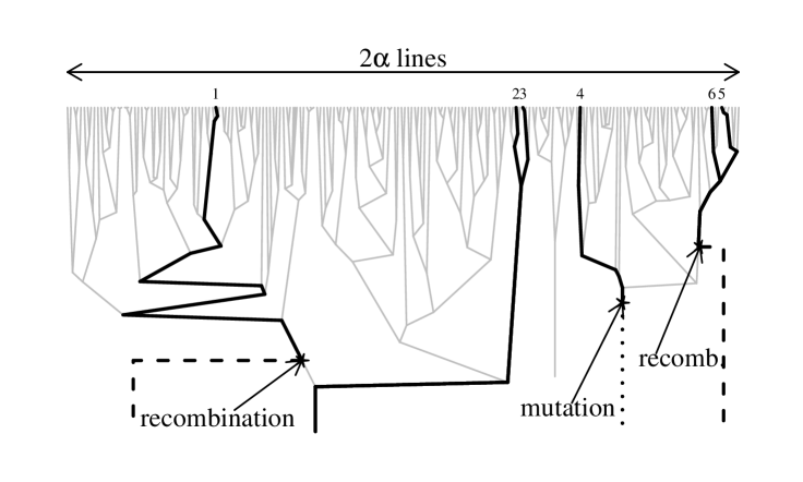
Figure 1: The Yule process approximation for the genealogy at the neutral locus in a sample of size $n=6$. The Yule process with immigration produces a random forest (grey lines) which grows from the past (past) to the present (top). A sample is drawn in the present. Every line is marked at constant rate along the Yule forest indicating recombination events. Sample individuals within the same tree not separated by a recombination mark share ancestry and thus belong to the same partition element of $\Upsilon$. In this realization, we find $\Upsilon=\{\{1\},\{2,3\},\{4\},\{5,6\}\}$.

Let us start with $\xi_{\beta_{0}}$ (see Figure 1 for an illustration of our approximation). Consider the selected site first. Take a Yule process with immigration. Starting with a single line,

• every line splits at rate $\alpha$.

• new lines (mutants) immigrate at rate $\alpha\theta$.

For this process we speak of Yule-time $i$ for the time the Yule process has $i$ lines for the first time. We stop this Yule process with immigration at Yule-time $\lfloor 2\alpha\rfloor$. In order to define identity by descent within a sample of $n$ lines, take a sample of $n$ randomly picked lines from the $\lfloor 2\alpha\rfloor$. Note that the Yule process with immigration defines a random forest $\mathcal{F}$ and we may define the random partition $\widetilde{\Upsilon}$ of $\{1,...,n\}$ by saying that

$$k\sim_{\widetilde{\Upsilon}}\ell\iff\,k,\ell\text{ are in the same tree of }\mathcal{F}.$$

As a special case of Theorem 1 we will show that $\widetilde{\Upsilon}$ is a good approximation to $\xi_{\beta_{0}}$ in the case $\rho=0$.

In order to extend the picture to the general case with recombination, consider a single line of the neutral allele at time $T$. The line may recombine in the interval $[T_{0},T]$ and thus have an ancestor at time $T_{0}$, which carries the wild-type allele. Since recombination events take place with a rate proportional to $\rho$ and $T-T_{0}=T^{\ast}$ is of the order $(\log\alpha)/\alpha$, it is natural to use the scaling

$$\rho=\gamma\frac{\alpha}{\log\alpha}.$$ (3.4)

Take a sample of $n$ lines from the $\lfloor 2\alpha\rfloor$ lines of the top of the Yule tree and consider the subtree of the $n$ lines. Indicating recombination events, we mark all branches in the subtree independently. A branch in the subtree, which starts at Yule-time $i_{1}$ and ends at Yule-time $i_{2}$ is marked with probability $1-p_{i_{1}}^{i_{2}}(\gamma,\theta)$, where

$$p_{i_{1}}^{i_{2}}(\gamma,\theta):=\exp\Big{(}-\frac{\gamma}{\log\alpha}\sum_{i=i_{1}+1}^{i_{2}}\frac{1}{i+\theta}\Big{)}.$$ (3.5)

Then, define the random partition $\Upsilon$ of $\{1,...,n\}$ (our approximation of $\xi_{\beta_{0}}$) by

$$k\sim_{\Upsilon}\ell\iff k\sim_{\widetilde{\Upsilon}}\ell\;\wedge\;\text{path from }k\text{ to }\ell\text{ in }\mathcal{F}\text{ not separated by a mark.}$$

To obtain an approximation of $\xi_{\geq\beta_{0}}$ consider the finite Kingman coalescent $\mathcal{C}:=(C_{t})_{t\geq 0}$. Given there are $m$ lines such that $C_{t}=C=\{C_{1},...,C_{m}\}$, transitions occur for $1\leq 1<j\leq m$ to

$$\big{(}C\setminus\{C_{i},C_{j}\}\big{)}\cup\{C_{i}\cup C_{j}\}\text{ with rate }1.$$

Given $\Upsilon$, our approximation of $\xi_{\geq\beta_{0}}$ is

$$\Upsilon\circ\mathcal{C}:=(\Upsilon\circ C_{t})_{t\geq 0}.$$

Remark 3.3.

Our approximations are formulated in terms of the total variation distance of probability measures. Given two probability measures $\mathbb{P},\mathbb{Q}$ on a $\sigma$-algebra $\mathcal{A}$, the total variation distance is given by

$$d_{TV}(\mathbb{P},\mathbb{Q})=\tfrac{1}{2}\sup_{A\in\mathcal{A}}|\mathbb{P}[A]-\mathbb{Q}[A]|.$$

Similarly, for two random variables $X,Y$ on $\Omega$ with $\sigma(X)=\sigma(Y)$ and distributions $\mathcal{L}(X)$ and $\mathcal{L}(Y)$ we will write

$$d_{TV}(X,Y)=d_{TV}(\mathcal{L}(X),\mathcal{L}(Y)).$$

Theorem 1.

1. The distribution of coalescent states $\xi_{\beta_{0}}$ at time $\beta_{0}$ under the full model can be approximated by a distribution of coalescent states of a Yule process with immigration. In particular,

   $$\mathbb{P}_{\alpha,\theta}[\xi_{\beta_{0}}^{B}=\emptyset]=1$$ (3.6)

   and the bound

   $$d_{TV}\big{(}\xi_{\beta_{0}}^{b},\Upsilon\big{)} =\mathcal{O}\Big{(}\frac{1}{(\log\alpha)^{2}}\Big{)}$$ (3.7)

   holds in the limit of large $\alpha$ and is uniform on compacta in $n,\gamma$ and $\theta$.

2. The distribution of genealogies $\xi_{\geq\beta_{0}}$ prior to the establishment of the beneficial allele can be approximated by the distribution of genealogies under a composition of a Yule process with immigration and the Kingman coalescent. In particular,

   $$\mathbb{P}[\xi_{\geq\beta_{0}}^{B}\neq(\emptyset)_{t\geq 0}]=\mathcal{O}\Big{(}\frac{1}{\alpha\log\alpha}\Big{)}$$

   and the bound

   $$d_{TV}\big{(}\xi_{\geq\beta_{0}}^{b},\Upsilon\circ\mathcal{C}\big{)} =\mathcal{O}\Big{(}\frac{1}{(\log\alpha)^{2}}\Big{)}$$ (3.8)

   holds in the limit of large $\alpha$ and is uniform on compacta in $n,\gamma$ and $\theta$.

Remark 3.4.

1. Let us give an intuitive explanation for the approximation of the genealogy at the selected site by $\widetilde{\Upsilon}$. Consider a finite population of size $N$. It is well-known that a supercritical branching process is a good approximation for the frequency path $\mathcal{X}$ at times $t$ when $X_{t}$ is small. In such a process, each individual branches at rate 1. It either splits in two with probability $\tfrac{1+s}{2}$ or dies with probability $\tfrac{1-s}{2}$. In this setting every line has a probability of $2s+\mathcal{O}(s^{2})\approx 2\alpha/N$ to be of infinite descent. In particular, new mutants that have an infinite line of descent arise approximately at rate $2s\cdot Nu=\alpha\theta/N$. In addition, when there are $2Ns$ lines of infinite descent there must be approximately $N$ lines in total, which is the whole population.

2. Using the approximation of $\xi_{\beta_{0}}$ by $\Upsilon$ we can immediately derive a result found in Pennings and Hermisson (2006b): when the Yule process has $i$ lines the probability that the next event (either a split of a Yule line or an incoming mutant) is a split is $\frac{i}{\theta+i}$, and that it is an incoming mutant is $\frac{\theta}{\theta+i}$. This implies that the random forest $\mathcal{F}$ is generated by Hoppe’s urn. Recall also the related Chinese restaurant process; see Aldous (1985) and Joyce and Tavaré (1987). The resulting sizes of all families is given by the Ewens’ Sampling Formula for the $\lfloor 2\alpha\rfloor$ lines when the Yule tree is stopped. Moreover, the Ewens’ Sampling Formula is consistent, i.e., subsamples of a large sample again follow the formula.

3. When biologists screen the genome of a sample for selective sweeps, they can not be sure to have sampled at time $t=T$. Given they have sampled lines linked to the beneficial type at $t<T$ when the beneficial allele is already in high frequency (e.g. $X_{t}\approx 1-\delta/\log\alpha$ for some $\delta>0$), the approximations of Theorem 1 still apply. The reason is that neither recombination events changing the genetical background nor coalescences occur in $[t;T]$ in $\xi$ with high probability; see Section 6.6. If $t>T$, a good approximation to the genealogy is $\widetilde{\mathcal{C}}\circ\Upsilon\circ\mathcal{C}$ where $\widetilde{\mathcal{C}}$ is a Kingman coalescent run for time $t-T$.

4. The model parameters $n,\gamma$ and $\theta$ enter the error terms $\mathcal{O}(.)$ above. The most severe error in (3.7) arises from ignoring events with two recombination events on a single line. See also Remark 5.4. Hence, $\gamma$ enters the error term quadratically. Since each line might have a double-recombination history, the sample size $n$ enters this error term linearly. The contribution of $\theta$ to the error term cannot be seen directly and is a consequence of the dependence of the frequency path $\mathcal{X}$ on $\theta$.

   Note that coalescence events always affect pairs of lines while both recombination and mutation affects only single lines. As a consequence, $n$ enters quadratically into higher order error terms. In particular, for practical purposes, the Yule process approximation becomes worse for big samples.

5. The proof of Theorem 1 can be found in Section 6. Key facts needed in the proof are collected in Section 5.

3.3 Application: Expected heterozygosity

The approximation of Theorem 1 using a Yule forest as a genealogy has direct consequences for the interpretation of population genetic data. While genealogical trees cannot be observed directly, their impact on measures of DNA sequence diversity in a population sample can be described. The idea is that mutations along the genealogy of a sample produce polymorphisms that can be observed. Genealogies in the neighbourhood of a recent adaptation event are shorter, on average, meaning that sequence diversity is reduced. This reduction is stronger, however, for a ’hard sweep’ (see Section 2.3), where the sample finds a common ancestor during the time of the selective phase $\mathbb{E}[T^{\ast}]\approx 2\log(\alpha)/\alpha\ll 1$ than for a ’soft sweep’, where the most recent common ancestor is older. Using our fine asymptotics for genealogies, we are able to quantify the prediction of sequence diversity under genetic hitchhiking with recurrent mutation. In this section we will concentrate on heterozygosity as the simplest measure of sequence diversity.

By definition, heterozygosity is the probability that two randomly picked lines from a population are different. Writing $H_{t}$ for the heterozygosity at time $t$ and using (3.6), we obtain

$$H_{T}=\mathbb{P}_{\alpha,\theta}[\xi_{\beta_{0}}^{b}=\{\{1\},\{2\}\}|\xi_{0}=(\{1\},\{2\},\emptyset)]\cdot H_{T_{0}}.$$

Assuming that the population was in equilibrium at time $0$, we can use Theorem 1, in particular (3.7), to obtain an approximation for the heterozygosity at time $T$.

Proposition 3.5.

Abbreviating $p_{i}:=p_{i}^{\lfloor 2\alpha\rfloor}(\gamma,\theta)$ (compare (3.5)), heterozygosity at time $T$ is approximated by

$$\frac{H_{T}}{H_{T_{0}}}=1-\frac{p_{1}^{2}}{\theta+1}-\frac{2\gamma}{\log\alpha}\sum_{i=2}^{\lfloor 2\alpha\rfloor}\frac{2i+\theta}{(i+\theta)^{2}(i+1+\theta)}p_{i}^{2}+\mathcal{O}\Big{(}\frac{1}{(\log\alpha)^{2}}\Big{)}$$ (3.9)

where the error is in the limit of large $\alpha$ and is uniform on compacta in $n,\gamma$ and $\theta$.

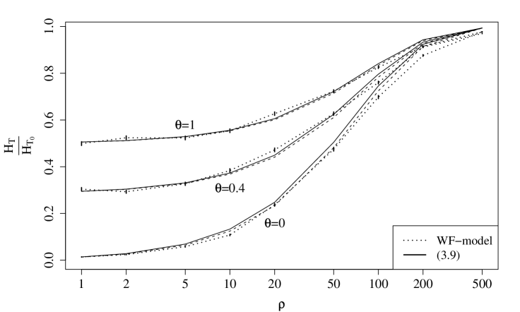
Figure 2: Reduction in heterozygosity at time of fixation of the beneficial allele. The $x$-axis shows the recombination distance of the selected from the neutral locus. Solid lines connect results from the analytical approximation. Dotted lines show simulation results of a structured coalescent in a Wright-Fisher model with $N=10^{4}$ and $\alpha=1000$. Small vertical bars indicate standard errors from $10^{3}$ numerical iterations.

Remark 3.6.

1. The formula (3.9) establishes that

   $$\frac{H_{T}}{H_{T_{0}}}=1-\frac{p_{1}^{2}}{\theta+1}+\mathcal{O}\Big{(}\frac{1}{\log\alpha}\Big{)}.$$ (3.10)

   In particular, to a first approximation, two lines taken from the population at time $T$ are identical by descent if their linked selected locus has the same origin (probability $\frac{1}{1+\theta}$) and if both lines were not hit by independent recombination events (probability $p_{1}^{2}$).

2. We investigated the quality of the approximation (3.9) by numerical simulations. The outcome can be seen in Figure 2. As we see, for $\alpha=1000$, our approximation works well for all values of $\theta\leq 1$ up to $\rho/\alpha=0.1$, i.e., $\gamma=0.7$.

3. We can compare Proposition 3.5 with the result for the heterozygosity under a star-like approximation for the genealogy at the selected site, which was used by Pennings and Hermisson (2006b, eq. (8)), i.e.

   $$\frac{H_{T}}{H_{T_{0}}}\approx 1-\frac{e^{-2\gamma}}{\theta+1}.$$ (3.11)

   Note that this formula also arises approximately by taking $p_{1}^{\lfloor 2\alpha\rfloor}(\gamma,0)$ instead of $p_{1}$ in (3.10). As shown in Table 2, the additional terms from the Yule process approximation lead to an improvement over the simple star-like approximation result.

   	$\theta=0,\rho=2$	$\theta=0,\rho=5$	$\theta=0,\rho=10$	$\theta=0,\rho=50$
   WF-model	0.024	0.058	0.108	0.475
   (3.9)	0.028(17%)	0.069(19%)	0.133(23%)	0.504(6%)
   (3.11)	0.032(33%)	0.079(36%)	0.151(40%)	0.559(18%)
   	$\theta=0.1,\rho=2$	$\theta=0.1,\rho=5$	$\theta=0.1,\rho=10$	$\theta=0.1,\rho=50$
   WF-model	0.112	0.153	0.223	0.507
   (3.9)	0.116(4%)	0.152(1%)	0.209(6%)	0.541(7%)
   (3.11)	0.12(7%)	0.162(6%)	0.228(2%)	0.599(18%)
   	$\theta=1,\rho=2$	$\theta=1,\rho=5$	$\theta=1,\rho=10$	$\theta=1,\rho=50$
   WF-model	0.524	0.523	0.554	0.723
   (3.9)	0.512(2%)	0.529(1%)	0.556(0%)	0.722(0%)
   (3.11)	0.516(2%)	0.539(3%)	0.575(4%)	0.779(8%)

   Table 2: Comparison of numerical simulation of a Wright-Fisher model to (3.9) and (3.11). Numbers in brackets are the relative error of the approximation. For $\theta=0$ and $\theta=1$, the same set of simulations as in Figure 2 are used. In particular, $N=10^{4}$ and $\alpha=1000$.

4. The quantification of sequence diversity patterns for selective sweeps with recurrent mutation using the Yule process approximation is not restricted to heterozygosity. Properties of several other statistics could be computed. As an example, we mention the site frequency spectrum, which describes the number of singleton, doubleton, tripleton, etc, mutations in the sample.

   Moreover, as pointed out by Pennings and Hermisson (2006b), selective sweeps with recurrent mutation also lead to a distinct haplotype pattern around the selected site. Intuitively, every beneficial mutant at the selected site brings along its own genetic background leading to several extended haplotypes. Quantifying such haplotypes patterns would require models for more than one neutral locus.

Proof of Proposition 3.5.

Using Theorem 1 we have to establish that $\mathbb{P}_{\alpha,\theta}[\xi_{\beta_{0}}^{b}=\{\{1,2\}\}|\xi_{0}=(\{1\},\{2\},\emptyset)]$ is approximately given by the right hand side of (3.5). To see this, we compute, accounting for all possibilities when coalescence of two lines can occur,

$$\mathbb{P}[\Upsilon=\{\{1,2\}\}] =\sum_{i=1}^{\lfloor 2\alpha\rfloor}\frac{i}{i+\theta}\frac{1}{\binom{i+1}{2}}p_{i}^{2}\cdot\prod_{j=i+1}^{\lfloor 2\alpha\rfloor}\Big{(}\frac{\theta}{j+\theta}\Big{(}1-\frac{2}{j+1}\Big{)}+\frac{j}{j+\theta}\Big{(}1-\frac{1}{\binom{j+1}{2}}\Big{)}\Big{)}$$

$$=\sum_{i=1}^{\lfloor 2\alpha\rfloor}\frac{2p_{i}^{2}}{(i+\theta)(i+1)}\cdot\prod_{j=i+1}^{\lfloor 2\alpha\rfloor}\Big{(}\theta\frac{j-1}{(j+\theta)(j+1)}+\frac{(j-1)(j+2)}{(j+\theta)(j+1)}\Big{)}$$

$$=\sum_{i=1}^{\lfloor 2\alpha\rfloor}\frac{2p_{i}^{2}}{(i+\theta)(i+1)}\cdot\prod_{j=i+1}^{\lfloor 2\alpha\rfloor}\frac{j-1}{j+1}\frac{j+2+\theta}{j+\theta}$$

$$=\sum_{i=1}^{\lfloor 2\alpha\lfloor}\frac{2p_{i}^{2}}{i+\theta}\frac{i}{(i+1+\theta)(i+2+\theta)}+\mathcal{O}\Big{(}\frac{1}{\alpha}\Big{)}$$

$$=\sum_{i=1}^{\lfloor 2\alpha\rfloor}\Big{(}\frac{2}{(i+1+\theta)(i+2+\theta)}-\frac{2\theta}{(i+\theta)(i+1+\theta)(i+2+\theta)}\Big{)}p_{i}^{2}+\mathcal{O}\Big{(}\frac{1}{\alpha}\Big{)}.$$

Rewriting gives

$$\mathbb{P}[\Upsilon=\{\{1,2\}\}] =\sum_{i=1}^{\lfloor 2\alpha\rfloor}\Big{(}\frac{2p_{i}^{2}}{i+1+\theta}-\frac{2p_{i}^{2}}{i+2+\theta}\Big{)}$$

$$\qquad\qquad\qquad\qquad-\theta\sum_{i=1}^{\lfloor 2\alpha\rfloor}\Big{(}\frac{p_{i}^{2}}{(i+\theta)(i+1+\theta)}-\frac{p_{i}^{2}}{(i+1+\theta)(i+2+\theta)}\Big{)}+\mathcal{O}\Big{(}\frac{1}{\alpha}\Big{)}$$

$$=\frac{2p_{1}^{2}}{\theta+2}+\sum_{i=1}^{\lfloor 2\alpha\rfloor}\frac{2(p_{i+1}^{2}-p_{i}^{2})}{i+2+\theta}$$

$$\qquad\qquad\qquad\qquad-\theta\frac{p_{1}^{2}}{(\theta+1)(\theta+2)}-\theta\sum_{i=1}^{\lfloor 2\alpha\rfloor}\frac{p_{i+1}^{2}-p_{i}^{2}}{(i+1+\theta)(i+2+\theta)}+\mathcal{O}\Big{(}\frac{1}{\alpha}\Big{)}$$

$$=\frac{p_{1}^{2}}{\theta+1}+\sum_{i=1}^{\lfloor 2\alpha\rfloor}\frac{2i+\theta+2}{(i+1+\theta)(i+2+\theta)}(p_{i+1}^{2}-p_{i}^{2})+\mathcal{O}\Big{(}\frac{1}{\alpha}\Big{)}$$

$$=\frac{p_{1}^{2}}{\theta+1}+\frac{2\gamma}{\log\alpha}\sum_{i=2}^{\lfloor 2\alpha\rfloor}p_{i}^{2}\frac{2i+\theta}{(i+\theta)^{2}(i+1+\theta)}+\mathcal{O}\Big{(}\frac{1}{(\log\alpha)^{2}}\Big{)}$$

where the last equality follows from

$$p_{i+1}^{2}-p_{i}^{2}=p_{i+1}^{2}\Big{(}1-\exp\Big{(}-\frac{2\gamma}{\log\alpha}\frac{1}{i+1+\theta}\Big{)}\Big{)}=p_{i+1}^{2}\frac{2\gamma}{\log\alpha}\frac{1}{i+1+\theta}+\frac{1}{i^{2}}\mathcal{O}\Big{(}\frac{1}{(\log\alpha)^{2}}\Big{)}.$$

∎

4 Proof of Proposition 3.1 (Fixation times)

Our calculations are based on the Green function $t(.;.)$ for the diffusion $\mathcal{X}=(X_{t})_{t\geq 0}$. This function satisfies

$$\mathbb{E}_{\alpha,\theta}^{p}\Big{[}\int_{0}^{T}f(X_{t})dt\Big{]}=\int_{0}^{1}t(x;p)f(x)dx$$ (4.1)

and

$$\mathbb{E}_{\alpha,\theta}^{p}\Big{[}\int_{0}^{T}\int_{t}^{T}f(X_{t})g(X_{s})dsdt\Big{]}=\int_{0}^{1}\int_{0}^{1}t(x;p)t(y;x)f(x)g(y)dydx.$$ (4.2)

Using

$$\psi_{\alpha,\theta}(y):=\psi(y):=\exp\Big{(}-2\int_{1}^{y}\frac{\mu_{\alpha,\theta}(z)}{\sigma^{2}(z)}dz\Big{)}=\frac{1}{y^{\theta}}\exp(2\alpha(1-y))$$

the Green function for $\mathcal{X}$, started in $p$, is given by (compare Ewens (2004), (4.40), (4.41))

$$t_{\alpha,\theta}(x;p) =\frac{2}{\sigma^{2}(x)\psi(x)}\int_{x\vee p}^{1}\psi(y)dy=\frac{2}{x(1-x)}\int_{x\vee p}^{1}e^{-2\alpha(y-x)}\Big{(}\frac{x}{y}\Big{)}^{\theta}dy.$$

Since $T^{\ast}$ depends only on the path conditioned not to hit 0, we need the Green function of the conditioned diffusion. To derive its infinitesimal characteristics, we need the absorption probability, i.e., given a current frequency of $p$ of the beneficial allele, its probability of absorption at 1 before hitting 0. This probability is given by

$$P^{1}_{\alpha,\theta}(p) =\frac{\int_{0}^{p}\psi(y)dy}{\int_{0}^{1}\psi(y)dy}=\frac{\int_{0}^{p}\frac{e^{-2\alpha y}}{y^{\theta}}dy}{\int_{0}^{1}\frac{e^{-2\alpha y}}{y^{\theta}}dy}$$

for $\theta<1$. For $\theta\geq 1$, we have $P^{1}_{\alpha,\theta}=1$, i.e., 0 is an inaccessible boundary. In the case $\theta<1$, the Green function of the conditioned process is for $p\leq x$ (compare Ewens (2004), (4.50))

$$t^{\ast}_{\alpha,\theta}(x;p)=P^{1}_{\alpha,\theta}(x)\cdot t_{\alpha,\theta}(x;p)$$

and for $x\leq p$ (see Ewens (2004), (4.49))

$$t^{\ast}_{\alpha,\theta}(x;p) =\frac{2}{\sigma^{2}(x)\psi(x)}\frac{(1-P^{1}_{\alpha,\theta}(x))P^{1}_{\alpha,\theta}(x)}{P^{1}_{\alpha,\theta}(p)}\int_{0}^{x}\psi(y)dy$$

$$=2\frac{1}{\sigma^{2}(x)\psi(x)}\frac{\int_{p}^{1}\psi(y)dy\int_{0}^{x}\psi(y)dy\int_{0}^{x}\psi(y)dy}{\int_{0}^{p}\psi(y)dy\int_{0}^{1}\psi(y)dy}.$$

Before we prove Proposition 3.1 we give some useful estimates.

Lemma 4.1.

1. For $\varepsilon,K\in(0;\infty)$ there exists $C\in\mathbb{R}$ such that

   $$\sup_{\varepsilon\leq x\leq 1,0\leq\theta\leq K}\Big{|}\frac{1-x^{\theta}}{\theta(1-x)}\Big{|}\leq C.$$ (4.3)

2. For $\theta\in[0;1)$,

   $$\int_{0}^{1}z^{-\theta}e^{-2\alpha z}dz=\frac{1}{2\alpha^{1-\theta}}\Gamma(1-\theta)+\mathcal{O}(e^{-2\alpha})$$ (4.4)

   where $\Gamma(.)$ is the Gamma function.

3. The bounds

   $$\int_{0}^{1}x^{\theta-1}e^{-2\alpha(1-x)}dx =\mathcal{O}\Big{(}\frac{1}{\alpha}\Big{)}+\frac{1}{\theta}\mathcal{O}\big{(}\alpha e^{-\alpha}\big{)},$$ (4.5)

   $$\int_{0}^{1}\frac{1-e^{-2\alpha x}}{x}dx-\log 2\alpha+\gamma_{e} =\mathcal{O}\Big{(}\frac{1}{\alpha}\Big{)},$$ (4.6)

   $$\int_{0}^{1}\frac{1-x^{\theta}}{1-x}e^{-2\alpha(1-x)}dx =\mathcal{O}\Big{(}\frac{1}{\alpha}\Big{)},$$ (4.7)

   $$\int_{0}^{1}\int_{0}^{y/2}\frac{1}{1-x}\Big{(}\frac{x}{y}\Big{)}^{\theta}e^{-2\alpha(y-x)}dxdy =\mathcal{O}\Big{(}\frac{1}{\alpha^{2}}\Big{)}$$ (4.8)

   hold in the limit of large $\alpha$, and uniformly on compacta in $\theta$.

Proof.

1. By a Taylor approximation of $x\mapsto x^{\theta}$ around $x=1$ we obtain

   $$x^{\theta}=1+\theta(1-x)+\tfrac{\theta(\theta-1)}{2}\xi^{\theta-2}(1-x)^{2}$$

   for some $x\leq\xi\leq 1$ and the result follows.

2. We simply compute

   $$\int_{0}^{1}z^{-\theta}e^{-2\alpha z}dz=\frac{1}{(2\alpha)^{1-\theta}}\int_{0}^{2\alpha}e^{-z}z^{-\theta}dz=\frac{1}{(2\alpha)^{1-\theta}}\Gamma(1-\theta)+\mathcal{O}(e^{-2\alpha})$$ (4.9)

3. For (4.5), we write

   $$\int_{0}^{1}x^{\theta-1}e^{-2\alpha(1-x)}dx =\frac{1}{\theta}x^{\theta}e^{-2\alpha(1-x)}\Big{|}_{0}^{1}+\frac{2\alpha}{\theta}\int_{0}^{1}x^{\theta}e^{-2\alpha(1-x)}dx$$

   $$=\frac{1}{\theta}-\frac{2\alpha}{\theta}\int_{0}^{1}e^{-2\alpha x}dx+\mathcal{O}\Big{(}\tfrac{2\alpha}{\theta}e^{-\alpha}+2\alpha\int_{0}^{1}(1-x)e^{-2\alpha(1-x)}dx\Big{)}$$

   $$=\mathcal{O}\Big{(}\frac{1}{\alpha}\Big{)}+\frac{1}{\theta}\mathcal{O}\big{(}\alpha e^{-\alpha}\big{)}$$

   where we have used 1. for $\varepsilon=\tfrac{1}{2}$. For (4.6), see (Bronstein, 1982, p. 61). Equation (4.7) follows from

   $$\int_{0}^{1}\frac{1-x^{\theta}}{1-x}e^{-2\alpha(1-x)}dx \leq\int_{0}^{1}\frac{1-x^{\lceil\theta\rceil}}{1-x}e^{-2\alpha(1-x)}dx=\sum_{i=0}^{\lceil\theta\rceil}\int_{0}^{1}x^{i}e^{-2\alpha(1-x)}dx\leq\frac{\lceil\theta\rceil}{2\alpha}$$

   and (4.8) from

   $$\int_{0}^{1}\int_{0}^{y/2}\frac{1}{1-x}\Big{(}\frac{x}{y}\Big{)}^{\theta}e^{-2\alpha(y-x)}dxdy \leq 2\int_{0}^{1}\int_{0}^{y/2}e^{-2\alpha(y-x)}dxdy$$

   $$=\frac{1}{2\alpha}\int_{0}^{1}e^{-2\alpha y}-e^{-2\alpha y/2}dy=\mathcal{O}\Big{(}\frac{1}{\alpha^{2}}\Big{)}.$$

∎

Lemma 4.2.

Let $2\alpha\geq 1$. There is $C>0$ such that for all $\theta\in[0;1]$ and $x\in[0;1]$

$$P^{1}_{\alpha,\theta}(x)\leq\big{(}C(2\alpha x)^{1-\theta}\big{)}\wedge 1.$$

Proof.

By a direct calculation, we find

$$P^{1}_{\alpha,\theta}(x) =\frac{\int_{0}^{2\alpha x}\frac{e^{-y}}{y^{\theta}}dy}{\int_{0}^{2\alpha}\frac{e^{-y}}{y^{\theta}}dy}\leq\frac{\int_{0}^{2\alpha x}y^{-\theta}}{\int_{0}^{1}\frac{e^{-1}}{y^{\theta}}}=e\cdot(2\alpha x)^{1-\theta}$$

Moreover, since $P^{1}_{\alpha,\theta}(x)$ is a probability, the bound $P^{1}_{\alpha,\theta}(x)\leq 1$ is obvious. ∎

Proof of Proposition 3.1.

We start with the proof of (3.1), i.e., we set $f=1$ in (4.1). We split the integral of $\mathbb{E}_{\alpha,\theta}[T]$ by using $\tfrac{1}{x(1-x)}=\tfrac{1}{x}+\tfrac{1}{1-x}$, i.e.,

$$\mathbb{E}_{\alpha,\theta}[T] =2\int_{0}^{1}\int_{0}^{y}\frac{1}{x}\Big{(}\frac{x}{y}\Big{)}^{\theta}e^{-2\alpha(y-x)}dxdy+2\int_{0}^{1}\int_{0}^{y}\frac{1}{1-x}\Big{(}\frac{x}{y}\Big{)}^{\theta}e^{-2\alpha(y-x)}dxdy.$$

For the first part,

$$2\int_{0}^{1} \int_{0}^{y}\frac{1}{x}\Big{(}\frac{x}{y}\Big{)}^{\theta}e^{-2\alpha(y-x)}dxdy\stackrel{{\scriptstyle x\to x/y}}{{=}}2\int_{0}^{1}\int_{0}^{1}x^{\theta-1}e^{-2\alpha y(1-x)}dydx$$

$$=\frac{1}{\alpha}\int_{0}^{1}x^{\theta-1}\frac{1}{1-x}\big{(}1-e^{-{2\alpha}(1-x)}\big{)}dx$$

$$=\frac{1}{\alpha}\int_{0}^{1}\Big{(}x^{\theta-1}+\frac{x^{\theta}}{1-x}\Big{)}\big{(}1-e^{-{2\alpha}(1-x)}\big{)}dx$$

$$=\frac{1}{\alpha}\Big{(}\frac{1}{\theta}-\int_{0}^{1}\frac{1-x^{\theta}}{1-x}(1-e^{-{2\alpha}(1-x)})dx+\int_{0}^{1}\frac{1-e^{-{2\alpha}(1-x)}}{1-x}dx\Big{)}+\mathcal{O}\Big{(}\frac{1}{\alpha^{2}}\Big{)}+\frac{1}{\theta}\mathcal{O}\big{(}\alpha e^{-\alpha}\big{)}$$

$$=\frac{1}{\alpha}\Big{(}\frac{1}{\theta}-\sum_{n=0}^{\infty}\int_{0}^{1}(x^{n}-x^{n+\theta})dx+\log({2\alpha})+\gamma_{e}\Big{)}+\mathcal{O}\Big{(}\frac{1}{\alpha^{2}}\Big{)}+\frac{1}{\theta}\mathcal{O}\big{(}{2\alpha}e^{-{\alpha}}\big{)}$$

$$=\frac{1}{\alpha}\Big{(}\frac{1}{\theta}-\theta\sum_{n=1}^{\infty}\frac{1}{n(n+\theta)}+\log({2\alpha})+\gamma_{e}\Big{)}+\mathcal{O}\Big{(}\frac{1}{\alpha^{2}}\Big{)}+\frac{1}{\theta}\mathcal{O}\big{(}\alpha e^{-{\alpha}}\big{)}.$$

where we have used (4.5) in the fourth and both, (4.6) and (4.7) in the fifth equality. The second part gives, using (4.8) and (4.3),

$$2\int_{0}^{1}\int_{0}^{y} \frac{1}{1-x}\Big{(}\frac{x}{y}\Big{)}^{\theta}e^{-{2\alpha}(y-x)}dxdy=2\int_{0}^{1}\int_{0}^{y/2}\frac{1}{1-x}\Big{(}\frac{x}{y}\Big{)}^{\theta}e^{-{2\alpha}(y-x)}dxdy$$ (4.10)

$$\qquad\qquad\qquad\qquad\qquad\qquad\qquad\qquad+2\int_{0}^{1}\int_{0}^{y/2}\frac{1}{1-y+x}\Big{(}1-\frac{x}{y}\Big{)}^{\theta}e^{-{2\alpha}x}dxdy$$

$$=2\int_{0}^{1}\int_{0}^{y}\frac{1}{1-y+x}e^{-{2\alpha}x}dxdy+\mathcal{O}\Big{(}\int_{0}^{1}\int_{0}^{y}\frac{x}{1+x}\Big{(}\frac{1}{1-y+x}+\frac{1}{y}\Big{)}e^{-{2\alpha}x}dxdy\Big{)}+\mathcal{O}\Big{(}\frac{1}{\alpha^{2}}\Big{)}$$

$$=2\int_{0}^{1}\int_{0}^{y}\frac{1}{1-x}e^{-{2\alpha}(y-x)}dydx+\mathcal{O}\Big{(}\int_{0}^{1}x\log\Big{(}\frac{y}{1-y+x}\Big{)}\Big{|}_{y=x}^{y=1}e^{-{2\alpha}x}dx\Big{)}+\mathcal{O}\Big{(}\frac{1}{\alpha^{2}}\Big{)}$$

$$=\frac{1}{\alpha}\int_{0}^{1}\frac{1-e^{-{2\alpha}(1-x)}}{1-x}dx+\mathcal{O}\Big{(}\frac{1}{\alpha^{2}}\int_{0}^{2\alpha}x\log\Big{(}\frac{2\alpha}{x}\Big{)}e^{-x}dx\Big{)}+\mathcal{O}\Big{(}\frac{1}{\alpha^{2}}\Big{)}$$

$$=\frac{1}{\alpha}\big{(}\log 2\alpha+\gamma_{e}\big{)}+\mathcal{O}\Big{(}\frac{\log\alpha}{\alpha^{2}}\Big{)}$$

and (3.1) follows. For the proof of (3.2) we have

$$\mathbb{E}_{\alpha,\theta}[T^{\ast}]=\frac{2\int_{0}^{1}\int_{x}^{1}\int_{0}^{x}\frac{e^{-2\alpha(y-x)}}{x(1-x)}\Big{(}\frac{x}{yz}\Big{)}^{\theta}e^{-2\alpha z}dzdydx}{\int_{0}^{1}z^{-\theta}e^{-2\alpha z}dz}$$ (4.11)

By using $\tfrac{1}{x(1-x)}=\tfrac{1}{x}+\tfrac{1}{1-x}$ we again split the integral in the numerator. For the $\tfrac{1}{x}$-part we find

$$2\int_{0}^{1}\int_{x}^{1}\int_{0}^{x} \frac{e^{-2\alpha(y-x)}}{x}\Big{(}\frac{x}{yz}\Big{)}^{\theta}e^{-2\alpha z}dzdydx\stackrel{{\scriptstyle x\to x/y}}{{=}}2\int_{0}^{1}\int_{0}^{1}\int_{0}^{xy}\frac{e^{-2\alpha(y(1-x))}}{x}\Big{(}\frac{x}{z}\Big{)}^{\theta}e^{-2\alpha z}dzdydx$$

$$\stackrel{{\scriptstyle z\to z/x}}{{=}}2\int_{0}^{1}\int_{0}^{1}\int_{0}^{y}e^{-2\alpha y(1-x)}z^{-\theta}e^{-2\alpha zx}dzdydx$$

$$=\frac{1}{\alpha}\int_{0}^{1}\int_{0}^{1}\frac{1}{1-x}\big{(}e^{-2\alpha z(1-x)}-e^{-2\alpha(1-x)}\big{)}z^{-\theta}e^{-2\alpha zx}dzdx$$

$$\stackrel{{\scriptstyle 1\to 1-x}}{{=}}\frac{1}{\alpha}\int_{0}^{1}\int_{0}^{1}\frac{1}{x}\big{(}e^{-2\alpha z}-e^{-2\alpha(x+z-xz)}\big{)}z^{-\theta}dzdx$$

$$=\frac{1}{\alpha}\int_{0}^{1}\frac{1-e^{-2\alpha x}}{x}dx\int_{0}^{1}e^{-2\alpha z}z^{-\theta}dz+\frac{1}{\alpha}\int_{0}^{1}\int_{0}^{1}\frac{1}{x}e^{-2\alpha(x+z)}\big{(}1-e^{2\alpha xz}\big{)}z^{-\theta}dxdz.$$

Using (4.4) we see that

$$\int_{0}^{1}\int_{0}^{1} \frac{1}{x}e^{-2\alpha(x+z)}\big{(}e^{2\alpha xz}-1\big{)}z^{-\theta}dxdz=\sum_{n=1}^{\infty}\int_{0}^{1}e^{-2\alpha z}z^{n-\theta}dz\int_{0}^{2\alpha}e^{-x}\frac{x^{n-1}}{n!}dx$$ (4.12)

$$=\mathcal{O}\Big{(}\int_{0}^{1}e^{-2\alpha z}z^{-\theta}\sum_{n=1}^{\infty}\frac{z^{n}}{n}dz\Big{)}$$

$$=\mathcal{O}\Big{(}\int_{0}^{1}e^{-2\alpha z}z^{-\theta}\log(1-z)dz\Big{)}$$

$$=\mathcal{O}\Big{(}\int_{0}^{1}z^{1-\theta}e^{-2\alpha z}dz\Big{)}$$

$$=\Gamma(2-\theta)\mathcal{O}\Big{(}\frac{1}{\alpha^{2-\theta}}\Big{)}$$

such that, with (4.4),

$$\frac{2\int_{0}^{1}\int_{x}^{1}\int_{0}^{x}\frac{e^{-\alpha(y-x)}}{x}\Big{(}\frac{x}{yz}\Big{)}^{\theta}e^{-\alpha z}dzdydx}{\int_{0}^{1}z^{-\theta}e^{-\alpha z}dz}=\frac{1}{\alpha}\big{(}\log 2\alpha+\gamma_{e}\big{)}+\mathcal{O}\Big{(}\frac{1}{\alpha^{2}}\Big{)}.$$ (4.13)

For the $\tfrac{1}{1-x}$-part, we write

$$\Big{|}\int_{0}^{1}\int_{x}^{1}\int_{0}^{x} \frac{e^{-2\alpha(y-x)}}{1-x}\Big{(}\frac{x}{yz}\Big{)}^{\theta}e^{-2\alpha z}dzdydx-\Big{(}\int_{0}^{1}z^{-\theta}e^{-2\alpha z}dz\Big{)}\Big{(}\int_{0}^{1}\int_{x}^{1}\frac{e^{-2\alpha(y-x)}}{1-x}\Big{(}\frac{x}{y}\Big{)}^{\theta}dydx\Big{)}\Big{|}$$

$$=\int_{0}^{1}\int_{x}^{1}\int_{x}^{1}\frac{e^{-2\alpha(y-x)}}{1-x}\Big{(}\frac{x}{yz}\Big{)}^{\theta}e^{-2\alpha z}dzdydx$$

$$=\mathcal{O}\Big{(}\int_{0}^{1}z^{-\theta}e^{-2\alpha z}\int_{0}^{z}\int_{x}^{1}\frac{e^{-2\alpha(y-x)}}{1-x}dydxdz\Big{)}$$

$$=\mathcal{O}\Big{(}\frac{1}{\alpha}\int_{0}^{1}z^{-\theta}e^{-2\alpha z}\int_{1-z}^{1}\frac{1-e^{-2\alpha x}}{x}dxdz\Big{)}$$

$$=\mathcal{O}\Big{(}\frac{1}{\alpha}\int_{0}^{1}z^{-\theta}e^{-2\alpha z}\log(1-z)dz\Big{)}$$

$$=\mathcal{O}\Big{(}\frac{1}{\alpha}\int_{0}^{1}z^{1-\theta}e^{-2\alpha z}dz\Big{)}$$

$$=\Gamma(2-\theta)\mathcal{O}\Big{(}\frac{1}{\alpha^{3-\theta}}\Big{)}$$

where we have used (4.4) in the last step. Hence, by (4.10),

$$\frac{2\int_{0}^{1}\int_{x}^{1}\int_{0}^{x}\frac{e^{-2\alpha(y-x)}}{1-x}\Big{(}\frac{x}{yz}\Big{)}^{\theta}e^{-2\alpha z}dzdydx}{\int_{0}^{1}z^{-\theta}e^{-2\alpha z}dz}=\frac{1}{\alpha}\big{(}\log 2\alpha+\gamma_{e}\big{)}+\theta\mathcal{O}\Big{(}\frac{\log\alpha}{\alpha^{2}}\Big{)}+\mathcal{O}\Big{(}\frac{1}{\alpha^{2}}\Big{)}.$$ (4.14)

Plugging (4.13) and (4.14) into (4.11) gives (3.2).

For the variance we start with $\theta<1$. By (4.2) and a similar calculation as in the proof of Lemma 4.2, for some finite $C$ (which is independent of $\theta$ and $\alpha$), using (4.2)

$$\mathbb{V}^{0} [T^{\ast}]=2\int_{0}^{1}\int_{0}^{w}t^{\ast}_{\theta}(w;0)t^{\ast}_{\theta}(x;w)dxdw$$ (4.15)

$$=4\int_{0}^{1}\int_{0}^{w}\frac{e^{2\alpha(w+x)}}{w^{1-\theta}(1-w)x^{1-\theta}(1-x)}\Big{(}\int_{w}^{1}\frac{e^{-2\alpha y}}{y^{\theta}}dy\Big{)}\Big{(}\int_{w}^{1}\frac{e^{-2\alpha z}}{z^{\theta}}dz\Big{)}\Big{(}\frac{\int_{0}^{x}\frac{e^{-2\alpha\hat{z}}}{\hat{z}^{\theta}}d\hat{z}}{\int_{0}^{1}\frac{e^{-2\alpha\tilde{z}}}{\tilde{z}^{\theta}}d\tilde{z}}\Big{)}^{2}dxdw$$

$$\begin{array}[]{c}\scriptstyle w,x,y,z\to\\[-4.30554pt] \leq\\[-4.30554pt] \scriptstyle 2\alpha(w,x,y,z)\end{array}\frac{C}{\alpha^{2}}\int_{0}^{2\alpha}\int_{0}^{w}\int_{w}^{1}\int_{w}^{1}\frac{e^{w+x-y-z}}{w(1-\frac{w}{2\alpha})x(1-\frac{x}{2\alpha})}\Big{(}\frac{wx}{yz}\Big{)}^{\theta}(x^{2-2\theta}\wedge 1)dzdydxdw$$

$$=\frac{2C}{\alpha^{2}}\int_{0}^{2\alpha}\int_{0}^{z}\int_{0}^{y}\int_{0}^{w}\Big{(}\frac{1}{w}+\frac{1}{2\alpha-w}\Big{)}\Big{(}\frac{1}{x}+\frac{1}{2\alpha-x}\Big{)}e^{w+x-y-z}\Big{(}\frac{wx}{yz}\Big{)}^{\theta}(x^{2-2\theta}\wedge 1)dxdwdydz$$

where the last equality follows by the symmetry of the integrand with respect to $y$ and $z$. We divide the last integral into several parts. Moreover, we use that

$$\int_{0}^{2\alpha}\int_{0}^{z}\int_{0}^{y}\int_{0}^{w}...dxdwdydz=\int_{0}^{2\alpha}\int_{0}^{z}\int_{0}^{y}\int_{0}^{w\wedge 1}...dxdwdydz+\int_{1}^{2\alpha}\int_{1}^{z}\int_{1}^{y}\int_{1}^{w}...dxdwdydz.$$ (4.16)

First,

$$\int_{0}^{2\alpha} \int_{0}^{z}\int_{0}^{y}\int_{0}^{w}\frac{1}{wx}e^{w+x-y-z}\Big{(}\frac{wx}{yz}\Big{)}^{\theta}(x^{2-2\theta}\wedge 1)dxdwdydz$$ (4.17)

$$=\mathcal{O}\Big{(}\int_{0}^{\infty}\int_{0}^{z}\int_{0}^{y}\int_{0}^{w\wedge 1}\frac{e^{-z}}{wx}\Big{(}\frac{wx}{yz}\Big{)}^{\theta}x^{2-2\theta}dxdwdydz+\int_{1}^{\infty}\int_{1}^{z}\int_{1}^{y}\int_{1}^{w}\frac{e^{w+x-y-z}}{wx}dxdwdydz\Big{)}$$

$$=\mathcal{O}\Big{(}\frac{1}{2-\theta}\int_{0}^{\infty}\int_{0}^{z}\int_{0}^{y}e^{-z}w\Big{(}\frac{1}{yz}\Big{)}^{\theta}dwdydz+\int_{1}^{\infty}\int_{x}^{\infty}\int_{w}^{\infty}\int_{y}^{\infty}\frac{e^{w+x-y-z}}{wx}dzdydwdx\Big{)}$$

$$=\mathcal{O}\Big{(}\int_{0}^{\infty}\int_{0}^{z}\frac{e^{-z}}{z^{\theta}}y^{2-\theta}dydz+\int_{1}^{\infty}\int_{x}^{\infty}\frac{e^{x-w}}{wx}dwdx\Big{)}$$

$$=\mathcal{O}\Big{(}\int_{0}^{\infty}z^{3-2\theta}e^{-z}dz+\int_{1}^{\infty}\frac{1}{x^{2}}dx\Big{)}=\mathcal{O}(1)$$

Second, since $\frac{1}{w(2\alpha-x)}\leq\frac{1}{x(2\alpha-w)}$ for $x\leq w$,

$$\int_{0}^{2\alpha} \int_{0}^{z}\int_{0}^{y}\int_{0}^{w}\Big{(}\frac{1}{w(2\alpha-x)}+\frac{1}{x(2\alpha-w)}\Big{)}e^{w+x-y-z}\Big{(}\frac{wx}{yz}\Big{)}^{\theta}(x^{2-2\theta}\wedge 1)dxdwdydz$$ (4.18)

$$=\mathcal{O}\Big{(}\int_{0}^{\infty}\int_{0}^{z}\int_{0}^{y}\int_{0}^{w\wedge 1}\frac{e^{-z}}{x(2\alpha-w)}\Big{(}\frac{wx}{yz}\Big{)}^{\theta}x^{2-2\theta}dxdwdydz$$

$$\qquad\qquad\qquad\qquad\qquad\qquad\qquad\qquad+\int_{1}^{2\alpha}\int_{1}^{z}\int_{1}^{y}\int_{1}^{w}\frac{e^{w+x-y-z}}{x({2\alpha}-w)}dxdwdydz\Big{)}$$

$$=\mathcal{O}\Big{(}\int_{0}^{2\alpha}\int_{0}^{z}\int_{0}^{y}\underbrace{\frac{w^{2}}{{2\alpha}-w}}_{\leq\frac{({2\alpha})^{2}}{{2\alpha}-w}-{2\alpha}}e^{-z}\Big{(}\frac{1}{yz}\Big{)}^{\theta}dwdydz+\int_{1}^{2\alpha}\int_{x}^{2\alpha}\int_{w}^{2\alpha}\int_{y}^{\infty}\frac{e^{w+x-y-z}}{x({2\alpha}-w)}dzdydwdx\Big{)}$$

$$=\mathcal{O}\Big{(}\alpha^{2}\int_{0}^{\infty}\int_{0}^{z}\big{(}-\log(1-\tfrac{y}{2\alpha})-\tfrac{y}{2\alpha}\big{)}e^{-z}\Big{(}\frac{1}{yz}\Big{)}^{\theta}dydz+\int_{1}^{2\alpha}\int_{x}^{2\alpha}\frac{e^{w+x}(e^{-2w}-e^{-4\alpha})}{x({2\alpha}-w)}dwdx\Big{)}$$

$$=\mathcal{O}\Big{(}\int_{0}^{\infty}\int_{0}^{z}y^{2-\theta}\frac{e^{-z}}{z^{\theta}}dydz+\int_{1}^{2\alpha}\int_{0}^{{2\alpha}-x}\frac{e^{-{2\alpha}+x}(e^{w}-e^{-w})}{wx}dwdx\Big{)}$$

$$=\mathcal{O}\Big{(}\int_{0}^{\infty}z^{3-2\theta}e^{-z}dz+\int_{1}^{{2\alpha}-1}\underbrace{\frac{1}{x({2\alpha}-x)}}_{=\frac{1}{2\alpha}\big{(}\frac{1}{x}+\frac{1}{{2\alpha}-x}\big{)}}dx\Big{)}+\mathcal{O}(1)$$

$$=\mathcal{O}(1).$$

Third,

$$\int_{0}^{2\alpha} \int_{0}^{z}\int_{0}^{y}\int_{0}^{w}\frac{1}{({2\alpha}-w)({2\alpha}-x)}e^{w+x-y-z}\Big{(}\frac{wx}{yz}\Big{)}^{\theta}(x^{2-2\theta}\wedge 1)dxdwdydz$$ (4.19)

$$\begin{array}[]{c}\scriptstyle(w,x,y,z)\to\\[-4.30554pt] =\\[-4.30554pt] \scriptstyle{2\alpha}-(w,x,y,z)\end{array}\mathcal{O}\Big{(}\int_{0}^{2\alpha}\int_{z}^{2\alpha}\int_{y}^{2\alpha}\int_{w}^{\infty}\frac{e^{y+z-x-w}}{wx}dxdwdydz\Big{)}$$

$$=\mathcal{O}\Big{(}\int_{0}^{2\alpha}\int_{0}^{x}\int_{0}^{w}\int_{0}^{y}\frac{e^{y+z-x-w}}{wx}dzdydwdx\Big{)}$$

$$=\mathcal{O}\Big{(}\int_{0}^{2\alpha}\int_{0}^{x}\frac{e^{-x}(e^{w}-e^{-w})}{xw}dwdx\Big{)}$$

$$=\mathcal{O}\Big{(}\int_{0}^{2\alpha}\int_{0}^{x\wedge 1}\frac{e^{-x}}{x}dwdx+\int_{1}^{2\alpha}\int_{1}^{x}\frac{e^{w-x}}{xw}dwdx\Big{)}=\mathcal{O}(1).$$

Plugging (4.17), (4.18), (4.19) into (4.15) gives (3.3) for $\theta<1$.

For $\theta\geq 1$, we compute

$$\mathbb{V}_{\alpha,\theta}[T^{\ast}] =\mathbb{V}_{\alpha,\theta}[T]=2\int_{0}^{1}\int_{0}^{w}\int_{w}^{1}\int_{w}^{1}\frac{e^{-{2\alpha}(w+x-y-z)}}{w(1-w)x(1-x)}\Big{(}\frac{wx}{yz}\Big{)}^{\theta}dzdydxdw$$ (4.20)

$$\leq 4\int_{0}^{1}\int_{0}^{z}\int_{0}^{y}\int_{0}^{w}\frac{e^{-{2\alpha}(w+x-y-z)}}{y(1-w)z(1-x)}dxdwdydz$$

$$\begin{array}[]{c}\scriptstyle(w,x,y,z)\to\\[-4.30554pt] =\\[-4.30554pt] \scriptstyle{2\alpha}(w,x,y,z)\end{array}\mathcal{O}\Big{(}\int_{0}^{2\alpha}\int_{0}^{z}\int_{0}^{y}\int_{0}^{w\wedge 1}\frac{e^{-z}}{y({2\alpha}-w)z({2\alpha}-x)}dxdwdydz$$

$$\qquad\qquad\qquad\qquad\qquad\qquad+\int_{1}^{2\alpha}\int_{x}^{2\alpha}\int_{w}^{2\alpha}\int_{y}^{\infty}\frac{e^{w+x-y-z}}{({2\alpha}-w)({2\alpha}-x)yz}dzdydwdx\Big{)}$$

$$=\mathcal{O}\Big{(}\frac{1}{\alpha}\int_{0}^{2\alpha}\int_{0}^{z}\int_{0}^{y}\frac{e^{-z}}{yz}\frac{w\wedge 1}{{2\alpha}-w}dwdydz+\int_{1}^{2\alpha}\int_{x}^{2\alpha}\int_{w}^{2\alpha}\frac{e^{w+x-2y}}{({2\alpha}-w)({2\alpha}-x)y^{2}}dydwdx\Big{)}$$

$$=\mathcal{O}\Big{(}\frac{1}{\alpha^{2}}\int_{0}^{2\alpha}\int_{0}^{z}\frac{e^{-z}}{z}\log\big{(}1-\tfrac{y}{2\alpha}\big{)}dydz+\int_{1}^{{2\alpha}-1}\int_{x}^{{2\alpha}-1}\frac{e^{x-w}}{({2\alpha}-w)({2\alpha}-x)w^{2}}dwdx+\frac{1}{\alpha^{2}}\Big{)}$$

$$=\mathcal{O}\Big{(}\frac{1}{\alpha^{2}}\int_{0}^{2\alpha}e^{-z}\log\big{(}1-\tfrac{z}{2\alpha}\big{)}dz+\int_{1}^{{2\alpha}-1}\Big{(}\frac{1}{({2\alpha}-x)x}\Big{)}^{2}dx+\frac{1}{\alpha^{2}}\Big{)}$$

$$=\mathcal{O}\Big{(}\frac{1}{\alpha^{2}}+\frac{1}{\alpha^{2}}\int_{1}^{{2\alpha}-1}\Big{(}\frac{1}{x}+\frac{1}{{2\alpha}-x}\Big{)}^{2}dx\Big{)}=\mathcal{O}\Big{(}\frac{1}{\alpha^{2}}\Big{)}.$$

∎

5 Key Lemmata

In this section we prove some key facts for the proof of Theorem 1. Recall $\rho=\gamma\frac{\log\alpha}{\alpha}$ from (3.4) and let $\xi_{1}^{\mathcal{X}},\xi_{2}^{\mathcal{X}},\xi_{3}^{\mathcal{X}},\xi_{4}^{\mathcal{X}},\xi_{5}^{\mathcal{X}}$ and $\xi_{6}^{\mathcal{X}}$ be Poisson-processes conditioned on $\mathcal{X}$ with rates $\tfrac{1}{X_{t}},\frac{\theta}{2}\frac{1-X_{t}}{X_{t}},\rho(1-X_{t}),\rho X_{t},1$ and $\frac{X_{t}}{1-X_{t}}$, at time $t$, as given in Table 3. Moreover, let $T_{i}^{\mathcal{X}}:=\sup\xi_{i}^{\mathcal{X}}$ be the last event of $\xi_{i}^{\mathcal{X}}$, $i=1,...,4$ in $[0;T]$.

Note that $\xi_{1}^{\mathcal{X}}$ give the pair coalescence rates in $B$. In addition, coalescences in the wild-type background might happen due to events in $\xi_{5}^{\mathcal{X}}\cup\xi_{6}^{\mathcal{X}}$ since $1+\frac{X_{t}}{1-X_{t}}=\frac{1}{1-X_{t}}$. The other processes determine changes in the genetic background due to mutation ($\xi_{2}^{\mathcal{X}}$) and recombination ($\xi_{3}^{\mathcal{X}},\xi_{4}^{\mathcal{X}}$).

process	$\xi_{1}^{\mathcal{X}}$	$\xi_{2}^{\mathcal{X}}$	$\xi_{3}^{\mathcal{X}}$	$\xi_{4}^{\mathcal{X}}$	$\xi_{5}^{\mathcal{X}}$	$\xi_{6}^{\mathcal{X}}$
rate	$\tfrac{1}{X_{t}}$	$\frac{\theta}{2}\frac{1-X_{t}}{X_{t}}$	$\rho(1-X_{t})$	$\rho X_{t}$	$1$	$\frac{X_{t}}{1-X_{t}}$
interpretation	coalescence in $B$	mutation from $B$ to $b$	recombination from $B$ to $b$	recombination from $b$ to $B$	coalescence in $b$

Table 3: Rates of Poisson processes

We will prove three Lemmata. The first deals with events of the Poisson processes during $[0;T_{0}]$. Recall that $T_{0}>0$ iff $\theta<1$. The second lemma is central for (3.6), i.e., to prove that no lines are in the beneficial background at time $T_{0}$. The third Lemma helps to order events during $[T_{0};T]$. We use the convention that $[s;t]=\emptyset$ for $s>t$.

Lemma 5.1.

Let $\theta<1$. Then,

$$\mathbb{P}^{0}_{\alpha,\theta}[\xi_{4}^{\mathcal{X}}\cap[0;T_{0}]\neq\emptyset] =\mathcal{O}\Big{(}\frac{1}{\alpha\log\alpha}\Big{)},$$ (5.1)

$$\mathbb{P}^{0}_{\alpha,\theta}[\xi_{6}^{\mathcal{X}}\cap[0;T_{0}]\neq\emptyset] =\mathcal{O}\Big{(}\frac{1}{\alpha^{2}}\Big{)}.$$ (5.2)

All error terms are in the limit for large $\alpha$, are uniform in $\theta$ and uniform on compacta in $\gamma$.

Lemma 5.2.

For all values of $\theta$ and $\alpha$,

$$\mathbb{P}^{0}_{\alpha,\beta}[\xi_{2}^{\mathcal{X}}\cap[T_{0};T_{0}+)=\emptyset]=0.$$

Lemma 5.3.

The bounds

$$\mathbb{P}^{0}_{\alpha,\theta}[\xi_{4}^{\mathcal{X}}\cap[T_{0};T_{2}^{\mathcal{X}}]\neq\emptyset] =\mathcal{O}\Big{(}\frac{1}{\sqrt{\alpha}}\Big{)},$$ (5.3)

$$\mathbb{P}^{0}_{\alpha,\theta}[\xi_{4}^{\mathcal{X}}\cap[T_{0};T_{3}^{\mathcal{X}}]\neq\emptyset] =\mathcal{O}\Big{(}\frac{1}{(\log\alpha)^{2}}\Big{)},$$ (5.4)

$$\mathbb{P}^{0}_{\alpha,\theta}[\xi_{5}^{\mathcal{X}}\cap[T_{0};T]\neq\emptyset] =\mathcal{O}\Big{(}\frac{\log\alpha}{\alpha}\Big{)},$$ (5.5)

$$\mathbb{P}^{0}_{\alpha,\theta}[\xi_{6}^{\mathcal{X}}\cap[T_{0};T_{2}^{\mathcal{X}}]\neq\emptyset] =\mathcal{O}\Big{(}\frac{1}{\sqrt{\alpha}}\Big{)},$$ (5.6)

$$\mathbb{P}^{0}_{\alpha,\theta}[\xi_{6}^{\mathcal{X}}\cap[T_{0};T_{3}^{\mathcal{X}}]\neq\emptyset] =\mathcal{O}\Big{(}\frac{\log\alpha}{\alpha}\Big{)}.$$ (5.7)

hold in the limit for large $\alpha$, are uniform on compacta in $\theta$ and $\gamma$.

Remark 5.4.

Lemmata 5.1 and 5.3 are crucial in ordering events in $\xi^{\mathcal{X}}$ (recall all rates from Table 1). In particular, let us consider events in $[T_{0};T]$, i.e., the bounds from Lemma 5.3. The full argument for the application of Lemmata 5.1-5.3 is given in the proof of Theorem 1 in Section 6. Consider a single line (i.e. a sample of size 1). Recall from Table 3 that the processes $\xi_{i}^{\mathcal{X}},i=2,3,4$ determine changes in the genetic background due to mutation ($\xi_{2}^{\mathcal{X}}$) and recombination ($\xi_{3}^{\mathcal{X}},\xi_{4}^{\mathcal{X}}$).

As we see from (5.4), the event that the line (backwards in time) changes background by recombination to the wild-type and back to the beneficial background has a probability of order $\mathcal{O}\big{(}\frac{1}{(\log\alpha)^{2}}\big{)}$. The event that the line changes genetic background by mutation and recombines back to the beneficial background has a probability of order $\mathcal{O}\big{(}\frac{1}{\sqrt{\alpha}}\big{)}$ by (5.3). The event of a coalescence in the wild-type background requires that both lines change background to the wild-type and so, necessarily, one event from (5.5), (5.6) or (5.7) must take place. Hence, the probability of a coalescence event in the wild-type background is of the order $\mathcal{O}\big{(}\frac{1}{\sqrt{\alpha}}\big{)}$.

Proof of Lemma 5.1.

For (5.1), since $P^{1}_{\theta}$ is monotone increasing in $\theta$ and $P_{\alpha,0}^{1}(p)=\frac{1-e^{-2\alpha p}}{1-e^{-2\alpha}}$, we compute, using Lemma 4.2 and $\rho=\mathcal{O}\big{(}\frac{\alpha}{\log\alpha}\big{)}$,

$$\mathbb{P}^{0}_{\alpha,\theta}[\xi_{4}^{\mathcal{X}}\cap[0;T_{0}]\neq\emptyset] =\mathbb{E}^{0}_{\alpha,\theta}\Big{[}1-\exp\Big{(}-\int_{0}^{T_{0}}\rho X_{t}dt\Big{)}\Big{]}\leq\mathbb{E}^{0}_{\alpha,\theta}\Big{[}\int_{0}^{T_{0}}\rho X_{t}dt\Big{]}$$

$$=\rho\int_{0}^{1}\big{(}t_{\alpha,\theta}(x;0)-t^{\ast}_{\alpha,\theta}(x;0)\big{)}xdx$$

$$\leq\rho\int_{0}^{1}(1-P^{1}_{\alpha,0}(x))xt_{\alpha,\theta}(x;0)dx$$

$$=\mathcal{O}\Big{(}\rho\int_{0}^{1}\int_{x}^{1}\frac{e^{-2\alpha y}}{1-x}\underbrace{\Big{(}\frac{x}{y}\Big{)}^{\theta}}_{\leq 1}dydx\Big{)}$$

$$=\mathcal{O}\Big{(}\frac{\rho}{\alpha}e^{-2\alpha}\int_{0}^{1}\frac{e^{2\alpha(1-x)}-1}{1-x}dx\Big{)}$$

$$=\mathcal{O}\Big{(}\frac{e^{-2\alpha}}{\log\alpha}\int_{0}^{2\alpha}\frac{e^{x}-1}{x}dx\Big{)}$$

$$=\mathcal{O}\Big{(}\frac{1}{\alpha\log\alpha}\Big{)}.$$

For $\xi_{6}^{\mathcal{X}}$, by a similar calculation,

$$\mathbb{P}^{0}_{\alpha,\theta}[\xi_{6}\cap[0;T_{0}]\neq\emptyset] \leq\int_{0}^{1}\big{(}t_{\alpha,\theta}(x;0)-t^{\ast}_{\alpha,\theta}(x;0)\big{)}\frac{x}{1-x}dx$$

$$=\mathcal{O}\Big{(}\int_{0}^{1}\int_{x}^{1}\frac{e^{-2\alpha y}(1-e^{-2\alpha(1-x)})}{(1-x)^{2}}\Big{(}\frac{x}{y}\Big{)}^{\theta}dydx\Big{)}$$

$$\leq\mathcal{O}\Big{(}\frac{1}{\alpha}e^{-2\alpha}\int_{0}^{1}\frac{(e^{2\alpha(1-x)}-1)(1-e^{-2\alpha(1-x)})}{(1-x)^{2}}dx\Big{)}$$

$$=\mathcal{O}\Big{(}e^{-2\alpha}\int_{0}^{2\alpha}\frac{(e^{x}-1)(1-e^{-x})}{x^{2}}dx\Big{)}$$

$$=\mathcal{O}\Big{(}\frac{1}{\alpha^{2}}\Big{)}.$$

∎

Proof of Lemma 5.2.

Note that the process $\mathcal{X}$ as well as its time-reversion $\mathcal{Z}=(Z_{t})_{t\geq 0}$ with $Z_{t}:=X_{T-t}$ are special cases of the diffusion studied in Taylor (2007). We use Lemma 2.1 of that paper, which extends Lemma 4.4 of Barton et al. (2004). Their Lemma 2.1 shows that, for all $0\leq s\leq T^{\ast}$,

$$\mathbb{P}_{\alpha,\theta}\Big{[}\int_{s}^{T^{\ast}}\frac{1-Z_{t}}{Z_{t}}dt=\infty\Big{]}=1.$$

In particular,

$$\mathbb{P}_{\alpha,\theta}[\xi_{2}^{\mathcal{X}}\cap[T_{0},T_{0}+s)=\emptyset]=\mathbb{E}_{\alpha,\theta}\Big{[}\exp\Big{(}-\int_{T_{0}}^{T_{0}+s}\frac{\theta}{2}\frac{1-X_{t}}{X_{t}}dt\Big{)}\Big{]}=0.$$

Hence the result follows for $s\to 0$. ∎

Proof of Lemma 5.3.

Proof of (5.3): Set $\mathcal{Y}=(Y_{t})_{0\leq t\leq T^{\ast}}$ with $Y_{t}=X_{T-t}$, i.e. $\mathcal{Y}$ is the time-reversion of $(X_{T_{0}+t})_{0\leq t\leq T^{\ast}}$. Recall that the Green function of the time-reversed diffusion $\mathcal{Y}$ is given for $x\leq p$ by (see Ewens (2004), (4.51))

$$t^{\ast\ast}(x;p)=2\frac{1}{\sigma^{2}(x)\psi(x)}\frac{\int_{x}^{1}\psi(y)dy\int_{0}^{x}\psi(y)dy}{\int_{0}^{1}\psi(y)dy}$$

and for $p\leq x$ by (see Ewens (2004), (4.52))

$$t^{\ast\ast}(x;p)=2\frac{1}{\sigma^{2}(x)\psi(x)}\frac{\int_{x}^{1}\psi(y)dy\int_{0}^{p}\psi(y)dy\int_{x}^{1}\psi(y)dy}{\int_{p}^{1}\psi(y)dy\int_{0}^{1}\psi(y)dy}$$

with the convention that $\frac{\int_{0}^{x}\psi(y)dy}{\int_{0}^{1}\psi(y)dy}=1$ for $\theta\geq 1$. Denote by

$$\widetilde{T}_{\varepsilon}^{\mathcal{X}}:=\sup\{{t\leq T:X_{t}=\varepsilon}\}=T-\inf\{t\geq 0:Y_{t}=\varepsilon\}.$$

We will use

$$\mathbb{P}_{\alpha,\theta}^{0}[\xi_{4}^{\mathcal{X}}\cap[T_{0};T_{2}^{\mathcal{X}}]\neq\emptyset]\leq\mathbb{P}_{\alpha,\theta}^{0}[\xi_{4}^{\mathcal{X}}\cap[T_{0};\widetilde{T}_{\varepsilon}^{\mathcal{X}}]\neq\emptyset]+\mathbb{P}_{\alpha,\theta}^{0}[\widetilde{T}^{\mathcal{X}}_{\varepsilon}\leq T_{2}^{\mathcal{X}}]$$ (5.8)

and bound both terms on the right hand side separately for $\varepsilon=\varepsilon(\alpha)=\frac{\log\alpha}{\sqrt{\alpha}}$. The bound of the first term is established by

$$\frac{\int_{x}^{1}\frac{e^{-2\alpha y}}{y^{\theta}}dy}{\int_{\varepsilon}^{1}\frac{e^{-2\alpha y}}{y^{\theta}}dy}=\mathcal{O}\Big{(}\Big{(}\frac{\varepsilon}{x}\Big{)}^{\theta}e^{-2\alpha(x-\varepsilon)}\Big{)}$$

uniformly for $\varepsilon\leq x\leq 1$ and

$$\mathbb{P}_{\alpha,\theta}^{0} [\xi_{4}^{\mathcal{X}}\cap[T_{0};\widetilde{T}_{\varepsilon}^{\mathcal{X}}]\neq\emptyset]=\mathbb{E}^{0}_{\alpha,\theta}\Big{[}1-\exp\Big{(}-\rho\int_{0}^{\widetilde{T}_{\varepsilon}^{\mathcal{X}}}X_{t}dt\Big{)}\Big{]}$$

$$=\mathbb{E}^{\varepsilon}_{\alpha,\theta}\Big{[}1-\exp\Big{(}-\rho\int_{0}^{\infty}Y_{t}dt\Big{)}\Big{]}\leq\rho\int_{0}^{1}t^{\ast\ast}_{\alpha,\theta}(x;\varepsilon)xdx$$

$$=\mathcal{O}\Big{(}\rho\int_{0}^{\varepsilon}\int_{x}^{1}\frac{1}{1-x}\Big{(}\frac{x}{y}\Big{)}^{\theta}e^{-2\alpha(y-x)}dydx+\rho\int_{\varepsilon}^{1}\int_{x}^{1}\frac{1}{1-x}\Big{(}\frac{\varepsilon}{y}\Big{)}^{\theta}e^{-2\alpha(y-\varepsilon)}dydx\Big{)}$$

$$=\mathcal{O}\Big{(}\rho\int_{0}^{\varepsilon}\int_{x}^{1}e^{-2\alpha(y-x)}dydx+\rho\int_{\varepsilon}^{1}\int_{\varepsilon}^{y}\frac{1}{1-x}e^{-2\alpha(y-\varepsilon)}dxdy\Big{)}$$

$$=\mathcal{O}\Big{(}\frac{\rho}{\alpha}\int_{0}^{\varepsilon}dx+\rho\int_{\varepsilon}^{1}\log\big{(}1-(y-\varepsilon)\big{)}e^{-2\alpha(y-\varepsilon)}dy\Big{)}$$

$$=\mathcal{O}\Big{(}\frac{1}{\sqrt{\alpha}}+\rho\int_{0}^{1}ye^{-2\alpha y}dy\Big{)}=\mathcal{O}\Big{(}\frac{1}{\sqrt{\alpha}}\Big{)},$$

while the bound of the second term follows from

$$\mathbb{P}_{\alpha,\theta}^{0}[\widetilde{T}^{\mathcal{X}}_{\varepsilon}\leq T_{2}^{\mathcal{X}}]=\mathbb{E}^{0}_{\alpha,\theta}\Big{[}1-\exp\Big{(}-\int_{\widetilde{T}^{\mathcal{X}}_{\varepsilon}}^{T}\frac{\theta}{2}\frac{1-X_{t}}{X_{t}}dt\Big{)}\Big{]}\leq\frac{\theta}{2}\frac{1}{\varepsilon}\mathbb{E}^{0}_{\alpha,\theta}[T^{\ast}]=\mathcal{O}\Big{(}\frac{1}{\sqrt{\alpha}}\Big{)}.$$ (5.9)

Hence, we have bounded both terms on the right hand side of (5.8) and thus have proved (5.3).

Proof of (5.4): Note that by (4.2)

$$\mathbb{P}^{0}_{\alpha,\theta} [\xi_{4}^{\mathcal{X}}\cap[T_{0};T_{3}^{\mathcal{X}}]\neq\emptyset]$$ (5.10)

$$=\mathbb{E}^{0}_{\alpha,\theta}\Big{[}\int_{T_{0}}^{T}\Big{(}1-\exp\Big{(}-\int_{T_{0}}^{t}\rho X_{s}ds\Big{)}\Big{)}\rho(1-X_{t})\exp\Big{(}-\int_{t}^{T}\rho(1-X_{s})ds\Big{)}dt\Big{]}$$

$$\leq\rho^{2}\mathbb{E}_{\alpha,\theta}^{0}\Big{[}\int_{T_{0}}^{T}(1-X_{t})\int_{T_{0}}^{t}X_{s}dsdt\Big{]}$$

$$=\rho^{2}\int_{0}^{1}\int_{0}^{1}t_{\theta}^{\ast}(x;0)t_{\theta}^{\ast}(y;x)x(1-y)dydx.$$

We split the last double integral into parts. First,

$$\int_{0}^{1}\int_{0}^{x}t_{\theta}^{\ast}(x;0)t_{\alpha,\theta}^{\ast}(y;x)x(1-y)dydx\leq\mathbb{V}^{0}_{\alpha,\theta}[T^{\ast}]=\mathcal{O}\Big{(}\frac{1}{\alpha^{2}}\Big{)}$$ (5.11)

by Proposition 3.1, (3.3). Second, recall $t_{\alpha,\theta}^{\ast}(y,x)=t_{\alpha,\theta}^{\ast}(y;0)$ for $x\leq y$. So we have, for all values of $\theta$,

$$\int_{0}^{1}\int_{x}^{1} t_{\alpha,\theta}^{\ast}(x;0)t_{\alpha,\theta}^{\ast}(y;0)x(1-y)dydx\leq\int_{0}^{1}\int_{x}^{1}t_{\alpha,\theta}(x;0)t_{\alpha,\theta}(y;0)x(1-y)dydx$$ (5.12)

$$=\mathcal{O}\Big{(}\int_{0}^{1}\int_{x}^{1}\int_{x}^{1}\int_{y}^{1}e^{-2\alpha(z+z^{\prime}-x-y)}\Big{(}\frac{xy}{zz^{\prime}}\Big{)}^{\theta}\frac{1}{1-x}\frac{1}{y}dz^{\prime}dzdydx\Big{)}$$

$$=\mathcal{O}\Big{(}\frac{1}{\alpha^{2}}\int_{0}^{2\alpha}\int_{x}^{2\alpha}\int_{x}^{2\alpha}\int_{y}^{2\alpha}e^{-(z+z^{\prime}-x-y)}\underbrace{\Big{(}\frac{xy}{zz^{\prime}}\Big{)}^{\theta}}_{\leq 1}\frac{1}{2\alpha-x}\frac{1}{y}dz^{\prime}dzdydx\Big{)}$$

$$=\mathcal{O}\Big{(}\frac{1}{\alpha^{2}}\int_{0}^{2\alpha}\int_{0}^{y}\frac{1}{2\alpha-x}\frac{1}{y}dxdy\Big{)}=\mathcal{O}\Big{(}\frac{1}{\alpha^{2}}\int_{0}^{2\alpha}\frac{\log(1-\tfrac{y}{2\alpha})}{y}dy\Big{)}$$

$$=\mathcal{O}\Big{(}\frac{1}{\alpha^{2}}\int_{0}^{1}\frac{\log(1-y)}{y}dy\Big{)}=\mathcal{O}\Big{(}\frac{1}{\alpha^{2}}\Big{)}.$$

Hence, plugging (5.11) and (5.12) into (5.10) establishes (5.4) since $\rho=\mathcal{O}\Big{(}\frac{\alpha}{\log\alpha}\Big{)}$.

Proof of (5.5): We simply observe, using Proposition 3.1,

$$\mathbb{P}^{0}_{\alpha,\theta}[\xi_{4}^{\mathcal{X}}\cap[T_{0};T]\neq\emptyset] =\mathbb{E}_{\alpha,\theta}^{0}[1-e^{-T^{\ast}}]\leq\mathbb{E}^{0}_{\alpha,\theta}[T^{\ast}]=\mathcal{O}\Big{(}\frac{\log\alpha}{\alpha}\Big{)}.$$

Proof of (5.6): We will use the time-reversed process $\mathcal{Y}$ as in the proof of (5.3). Note that

$$\mathbb{P}_{\alpha,\theta}^{0}[\xi_{6}^{\mathcal{X}}\cap[T_{0};T_{2}^{\mathcal{X}}]\neq\emptyset]\leq\mathbb{P}_{\alpha,\theta}^{0}[\xi_{6}^{\mathcal{X}}\cap[T_{0};\widetilde{T}_{\varepsilon}^{\mathcal{X}}]\neq\emptyset]+\mathbb{P}_{\alpha,\theta}^{0}[\widetilde{T}^{\mathcal{X}}_{\varepsilon}\leq T_{2}^{\mathcal{X}}]$$ (5.13)

and the last term is bounded by (5.9). The first term is bounded using

$$\frac{1}{\int_{\varepsilon}^{1}\frac{e^{-2\alpha y}}{y^{\theta}}dy}=\mathcal{O}\big{(}\alpha\varepsilon^{\theta}e^{2\alpha\varepsilon}\big{)}$$

by (recall $\varepsilon=\varepsilon(\alpha)=\frac{\log\alpha}{\sqrt{\alpha}}$)

$$\mathbb{P}_{\alpha,\theta}^{0} [\xi_{6}^{\mathcal{X}}\cap[T_{0};\widetilde{T}_{\varepsilon}^{\mathcal{X}}]\neq\emptyset]\leq\int_{0}^{1}t^{\ast\ast}_{\alpha,\theta}(x;\varepsilon)\frac{x}{1-x}dx$$

$$=\mathcal{O}\Big{(}\int_{0}^{\varepsilon}\int_{x}^{1}\frac{1}{(1-x)^{2}}\Big{(}\frac{x}{y}\Big{)}^{\theta}e^{-2\alpha(y-x)}dydx$$

$$\qquad\qquad\qquad\qquad\qquad+\alpha\int_{\varepsilon}^{1}\int_{x}^{1}\int_{x}^{1}\frac{1}{(1-x)^{2}}\Big{(}\frac{x\varepsilon}{yz}\Big{)}^{\theta}e^{-2\alpha(y+z-x-\varepsilon)}dzdydx\Big{)}$$

$$=\mathcal{O}\Big{(}\int_{0}^{\varepsilon}\int_{x}^{1}e^{-2\alpha(y-x)}dydx+\frac{1}{\alpha}\int_{\varepsilon}^{1}e^{-2\alpha(x-\varepsilon)}dx\Big{)}$$

$$=\mathcal{O}\Big{(}\frac{\log\alpha}{\alpha^{3/2}}+\frac{1}{\alpha^{2}}\Big{)}=\mathcal{O}\Big{(}\frac{\log\alpha}{\alpha^{3/2}}\Big{)}.$$

Proof of (5.7): Note that

$$\mathbb{P}^{0}[\xi_{6}^{\mathcal{X}}\cap[T_{0};T_{3}^{\mathcal{X}}]\neq\emptyset] \leq\rho\int_{0}^{1}\int_{0}^{1}t_{\theta}^{\ast}(w;0)t_{\theta}^{\ast}(x;w)\frac{w}{1-w}(1-x)dxdw.$$

We split the last integral and use that $t^{\ast}(x;w)=t^{\ast}(x;0)$ for $w\leq x$, such that

$$\int_{0}^{1}\int_{w}^{1}t_{\alpha,\theta}^{\ast}(w;0)t_{\alpha,\theta}^{\ast}(x;0)\frac{w}{1-w}(1-x)dxdw \leq\mathcal{O}\Big{(}\Big{(}\int_{0}^{1}t_{\alpha,\theta}^{\ast}(w;0)dw\Big{)}^{2}\Big{)}$$

$$=\mathcal{O}\big{(}(\mathbb{E}_{\alpha,\theta}^{0}[T^{\ast}])^{2}\big{)}=\mathcal{O}\Big{(}\frac{(\log\alpha)^{2}}{\alpha^{2}}\Big{)}$$

by Proposition 3.1. For the second part, using (4.16), we have in the case $\theta<1$, by a calculation similar to (4.18),

$$\int_{0}^{1}\int_{0}^{w} t_{\alpha,\theta}^{\ast}(w;0)t_{\alpha,\theta}^{\ast}(x;w)\frac{w}{1-w}(1-x)dxdw$$ (5.14)

$$=\mathcal{O}\Big{(}\int_{0}^{1}\int_{0}^{w}\int_{w}^{1}\int_{w}^{1}\frac{e^{2\alpha(w+x-y-z)}}{(1-w)^{2}x}\Big{(}\frac{wx}{yz}\Big{)}^{\theta}(2\alpha x\wedge 1)^{2-2\theta}dzdydxdw\Big{)}$$

$$=\mathcal{O}\Big{(}\frac{1}{\alpha}\int_{0}^{2\alpha}\int_{0}^{z}\int_{0}^{y}\int_{0}^{w}\frac{e^{w+x-y-z}}{x(2\alpha-w)^{2}}\Big{(}\frac{wx}{yz}\Big{)}^{\theta}(x\wedge 1)^{2-2\theta}dxdwdydz\Big{)}$$

$$=\mathcal{O}\Big{(}\frac{1}{\alpha}\int_{0}^{2\alpha}\int_{0}^{z}\int_{0}^{y}\int_{0}^{w\wedge 1}\frac{e^{-z}}{x(2\alpha-w)^{2}}\Big{(}\frac{wx}{yz}\Big{)}^{\theta}x^{2-2\theta}dxdwdydz$$

$$\qquad\qquad\qquad\qquad\qquad+\frac{1}{\alpha}\int_{1}^{2\alpha}\int_{x}^{2\alpha}\int_{w}^{2\alpha}\int_{y}^{2\alpha}\frac{e^{w+x-y-z}}{x(2\alpha-w)^{2}}dzdydwdx\Big{)}$$

$$=\mathcal{O}\Big{(}\frac{1}{\alpha}\int_{0}^{2\alpha}\int_{0}^{z}\int_{0}^{y}\frac{e^{-z}w^{2}}{(2\alpha-w)^{2}}\frac{1}{(yz)^{\theta}}dwdydz$$

$$\qquad\qquad\qquad\qquad\qquad+\frac{1}{\alpha}\int_{1}^{2\alpha}\int_{x}^{2\alpha}\int_{w}^{2\alpha}\frac{e^{w+x-y}(e^{-y}-e^{-2\alpha})}{x(2\alpha-w)^{2}}dydwdx\Big{)}$$

$$=\mathcal{O}\Big{(}\frac{1}{\alpha^{3}}\int_{0}^{2\alpha}\int_{0}^{z}\int_{0}^{y\wedge\alpha}\frac{e^{-z}w^{2}}{(yz)^{\theta}}dwdydz+e^{-\alpha}\alpha^{1-2\theta}\int_{\alpha}^{2\alpha}\int_{w}^{2\alpha}\int_{w}^{2\alpha}\frac{1}{(2\alpha-w)^{2}}dzdydw$$

$$\qquad\qquad\qquad\qquad+\frac{1}{\alpha}\int_{1}^{2\alpha}\int_{x}^{2\alpha}\frac{e^{w+x}(\tfrac{1}{2}(e^{-2w}-e^{-4\alpha})-e^{-w-2\alpha}+e^{-4\alpha})}{x(2\alpha-w)^{2}}dwdx\Big{)}$$

$$\stackrel{{\scriptstyle w\to 2\alpha-w}}{{=}}\mathcal{O}\Big{(}\frac{1}{\alpha^{3}}\int_{0}^{2\alpha}e^{-z}z^{4-2\theta}dz$$

$$\qquad\qquad\qquad\qquad\qquad+\frac{e^{-4\alpha}}{\alpha}\int_{1}^{2\alpha}\int_{0}^{2\alpha-x}\frac{e^{2\alpha-w+x}(\tfrac{1}{2}(e^{2w}-1)-e^{w}+1)}{xw^{2}}dwdx\Big{)}$$

$$=\mathcal{O}\Big{(}\frac{1}{\alpha^{3}}+\frac{1}{\alpha}\int_{1}^{2\alpha-1}\frac{e^{-2x}}{x(2\alpha-x)^{2}}dx\Big{)}=\mathcal{O}\Big{(}\frac{1}{\alpha^{3}}\Big{)}.$$

For $\theta\geq 1$, we compute, similar to (4.20),

$$\int_{0}^{1}\int_{0}^{w} t_{\alpha,\theta}^{\ast}(w;0)t_{\alpha,\theta}^{\ast}(x;w)\frac{w}{1-w}(1-x)dxdw=\int_{0}^{1}\int_{0}^{w}\int_{w}^{1}\int_{w}^{1}\frac{e^{{2\alpha}(w+x-y-z)}}{(1-w)^{2}x}\Big{(}\frac{wx}{yz}\Big{)}^{\theta}dzdydxdw$$

$$\begin{array}[]{c}\scriptstyle(w,x,y,z)\to\\[-4.30554pt] \leq\\[-4.30554pt] \scriptstyle{2\alpha}(w,x,y,z)\end{array}\mathcal{O}\Big{(}\frac{1}{\alpha}\int_{0}^{2\alpha}\int_{0}^{z}\int_{0}^{y}\int_{0}^{w}\frac{e^{w+x-y-z}}{(2\alpha-w)^{2}}\frac{w}{yz}dxdwdydz\Big{)}$$

$$=\mathcal{O}\Big{(}\frac{1}{\alpha}\int_{0}^{2\alpha}\int_{0}^{z}\int_{0}^{y}\int_{0}^{w\wedge 1}\frac{e^{-z}w}{({2\alpha}-w)^{2}yz}dxdwdydz$$

$$\qquad\qquad\qquad\qquad\qquad\qquad+\frac{1}{\alpha}\int_{1}^{2\alpha}\int_{x}^{2\alpha}\int_{w}^{2\alpha}\int_{y}^{2\alpha}\frac{e^{w+x-y-z}w}{(2\alpha-w)^{2}yz}dzdydwdx\Big{)}$$

$$=\mathcal{O}\Big{(}\frac{1}{\alpha^{3}}\int_{0}^{2\alpha}\int_{0}^{z}\int_{0}^{y\wedge\alpha}e^{-z}dwdydz+\frac{1}{\alpha}\int_{1}^{2\alpha}\int_{x}^{2\alpha}\int_{w}^{2\alpha}\int_{y}^{2\alpha}\frac{e^{w+x-y-z}}{(2\alpha-w)^{2}x}dzdydwdx\Big{)}$$

$$=\mathcal{O}\Big{(}\frac{1}{\alpha^{3}}\Big{)},$$

since the last term in the second to last line equals the term in the fifth line of (5.14) such that we are done. ∎

6 Proof of Theorem 1

Recall the transition rates of the process $\xi^{\mathcal{X}}$ given in Table 1. We prove Theorem 1 in four steps. First, we establish that almost surely, all lines in $\xi^{\mathcal{X}}$ are in the wild-type background by time $\beta_{0}$. In Step 2, we give an approximate structured coalescent $\eta^{\mathcal{X}}$, which has different rates before and after $\beta_{0}$. This process already provides us with a good approximation for $\xi_{\geq\beta_{0}}$. In Step 3, we will use a random time-change of the diffusion $\mathcal{X}$ to a supercritical Feller diffusion $\mathcal{Y}$ with immigration. In Step 4 we will use facts about the connection of the supercritical branching process with immigration to a Yule process with immigration.

6.1 Step 1: All lines in wild-type background by time $\beta_{0}$

We will show below that all lines in the structured coalescent $\xi^{\mathcal{X}}$ are in the wild-type background by time $\beta_{0}$.

Proposition 6.1.

For all values of $\theta,\alpha$,

$$\mathbb{P}_{\alpha,\theta}[\xi_{\beta_{0}}^{B}=\emptyset]=1.$$

Proof.

Note that the structured coalescent $\xi^{\mathcal{X}}$ can be constructed using a finite number of processes $\xi_{1}^{\mathcal{X}},\xi_{2}^{\mathcal{X}},\xi_{3}^{\mathcal{X}},\xi_{4}^{\mathcal{X}}$ (compare Table 3). In particular, the escape of lines in the beneficial background to the wild-type background due to mutation is given by the processes $\xi_{2}^{\mathcal{X}}$. Moreover, we know from Lemma 5.2 that any line in the beneficial background by time $T_{0}+\varepsilon$ for some $\varepsilon>0$ will experience such an escape since $\xi_{2}^{\mathcal{X}}\cap[T_{0};T_{0}+]\neq\emptyset$ almost surely. Hence the assertion follows. ∎

6.2 Step 2: Approximation of $\xi_{\geq 0}$ by $\eta_{\geq 0}$

In order to define the process $\eta^{\mathcal{X}}$ we use transition rates as given in Tables 4 and 5. Moreover, set

$$\eta_{\geq s}:=\int\mathbb{P}_{\alpha,\theta}[d\mathcal{X}](\eta_{s+t}^{\mathcal{X}})_{t\geq 0}.$$

We will establish that $\xi_{\geq 0}$ and $\eta_{\geq 0}$ are close in variational distance.

Proposition 6.2.

The bound

$$d_{TV}(\xi_{\geq 0},\eta_{\geq 0})=\mathcal{O}\Big{(}\frac{1}{(\log\alpha)^{2}}\Big{)}.$$

holds in the limit of large $\alpha$ and uniformly on compacta in $n,\gamma$ and $\theta$.

Remark 6.3.

Note that $(\eta^{\mathcal{X}}_{t})_{t\geq\beta_{0}}$ does not depend on $\mathcal{X}$ (i.e. $\eta_{\geq\beta_{0}}=(\eta^{\mathcal{X}}_{t})_{t\geq\beta_{0}}$ in distribution for all realizations of $\mathcal{X}$). Using the same argument as in Step 1 all lines of $\eta_{\beta_{0}}$ are in the wild-type background. These two facts together imply that $\xi_{\geq\beta_{0}}$ approximately has the same transition rates as the finite Kingman coalescent $\mathcal{C}$, which is the statement of (3.8).

event	coal in $B$	coal in $b$	mut from $B$ to $b$	rec from $B$ to $b$	rec from $b$ to $B$
rate	$\frac{1-X_{t}}{X_{t}}$	$0$	$\frac{\theta}{2}\frac{1-X_{t}}{X_{t}}$	$\rho(1-X_{t})$	$0$

Table 4: Transition rates of $\eta^{\mathcal{X}}$ in the interval $[0;\beta_{0}]$.

event	coal in $B$	coal in $b$	mut from $B$ to $b$	rec from $B$ to $b$	rec from $b$ to $B$
rate	$0$	$1$	$0$	$0$	$0$

Table 5: Transition rates of $\eta^{\mathcal{X}}$ in the interval $[\beta_{0};\infty]$.

Proof of Proposition 6.2.

Again it is important to note that $\xi^{\mathcal{X}}$ can be constructed using a finite number of Poisson processes $\xi_{1}^{\mathcal{X}},...,\xi_{6}^{\mathcal{X}}$. In the same way, $\eta^{\mathcal{X}}$ can be constructed using a finite number of Poisson processes $\xi_{1}^{\mathcal{X}},\xi_{2}^{\mathcal{X}},\xi_{3}^{\mathcal{X}},\xi_{5}^{\mathcal{X}}$ and Poisson processes with rates $\frac{1-X_{t}}{X_{t}}$.

Consider times $0\leq\beta\leq\beta_{0}$ first and recall $T_{i}^{\mathcal{X}}=\sup\xi_{i}^{\mathcal{X}}$. A single line may escape the beneficial background and recombine back in $\xi^{\mathcal{X}}$, while this is not possible in $\eta^{\mathcal{X}}$. Such an event in $\xi^{\mathcal{X}}$ requires that either $\xi_{4}^{\mathcal{X}}\cap[T_{0};T_{2}^{\mathcal{X}}]\neq\emptyset$ or $\xi_{4}^{\mathcal{X}}\cap[T_{0};T_{3}^{\mathcal{X}}]\neq\emptyset$ for one triple of the processes $\xi_{2}^{\mathcal{X}},\xi_{3}^{\mathcal{X}},\xi_{4}^{\mathcal{X}}$, which has a probability of order $\mathcal{O}\Big{(}\frac{1}{(\log\alpha)^{2}}\Big{)}$ by (5.3) and (5.4). Hence, ignoring these events produces a total variation distance of at most $\mathcal{O}\Big{(}\frac{1}{(\log\alpha)^{2}}\Big{)}$. The coalescence rates in the beneficial background of the processes $\xi^{\mathcal{X}}$ and $\eta^{\mathcal{X}}$ differ by 1. By the bound (5.5), the different coalescence rates in the beneficial background produce a total variation distance of $\mathcal{O}\big{(}\frac{\log\alpha}{\alpha}\big{)}$. Lastly, since $\frac{1}{1-X_{t}}=1+\frac{X_{t}}{1-X_{t}}$, we can assume that coalescences in the wild-type background in $\xi^{\mathcal{X}}$ occur along events of one pair of processes $\xi_{5}^{\mathcal{X}}\cup\xi_{6}^{\mathcal{X}}$. Such an event requires that either $\xi_{5}^{\mathcal{X}}\cap[T_{0};T]\neq\emptyset$, $\xi_{6}^{\mathcal{X}}\cap[T_{0};T_{2}^{\mathcal{X}}]\neq\emptyset$ or $\xi_{6}^{\mathcal{X}}\cap[T_{0};T_{3}^{\mathcal{X}}]\neq\emptyset$. These events together have a probability of order $\mathcal{O}\big{(}\frac{1}{\sqrt{\alpha}}\big{)}$ by (5.5), (5.6) and (5.7) and hence, ignoring these events gives a total variation distance of order $\mathcal{O}\big{(}\frac{1}{\sqrt{\alpha}}\big{)}$. Hence, $\xi^{\mathcal{X}}$ and $\eta^{\mathcal{X}}$ are close for times $0\leq\beta\leq\beta_{0}$.

Let us turn to times $\beta\geq\beta_{0}$. It is important to notice that, using the same arguments as in the proof of Proposition 6.1, $\mathbb{P}_{\alpha,\theta}[\eta_{\beta_{0}}^{B}=\emptyset]=1$. Note that $\eta^{\mathcal{X}}$ differs from $\xi^{\mathcal{X}}$ by ignoring back-recombinations along processes $\xi^{\mathcal{X}}_{4}$ and by changing the coalescence rate in the wild-type background from $\frac{1}{1-X_{t}}$ to 1. Considering a single line, ignoring events in $\xi^{\mathcal{X}}_{4}$ produces a total variation distance of order $\mathcal{O}\big{(}\frac{1}{\alpha\log\alpha}\big{)}$ by (5.1). Hence, we can assume that all lineages are in the wild-type background for $\beta\geq\beta_{0}$. For coalescences in the wild-type background, we are using that $\frac{1}{1-X_{t}}=1+\frac{X_{t}}{1-X_{t}}$ and the fact that ignoring events, which occur along one process $\xi_{6}^{\mathcal{X}}$ produces a total variation distance of order $\mathcal{O}\big{(}\frac{1}{\alpha^{2}}\big{)}$ by (5.2).

Putting all arguments together, we have

$$d_{TV}(\xi_{\geq 0},\eta_{\geq 0})\leq d_{TV}(\xi_{0\leq\beta\leq\beta_{0}},\eta_{0\leq\beta\leq\beta_{0}})+d_{TV}(\xi_{\geq\beta_{0}},\eta_{\geq\beta_{0}})=\mathcal{O}\Big{(}\frac{1}{(\log\alpha)^{2}}\Big{)}.$$

∎

6.3 Step 3: Random time-change to a supercritical branching process

By a random time change, the diffusion (2.1) is taken to a supercritical branching process with immigration. Specifically, use the random time change $d\tau=(1-X_{t})dt$ to see that the time-changed process $\mathcal{Y}=(Y_{\tau})_{\tau\geq 0}$ solves

$$dY=\big{(}\tfrac{\theta}{2}+\alpha Y\big{)}d\tau+\sqrt{Y}d\widetilde{W},$$ (6.1)

stopped when $Y_{\tau}=1$, with some Brownian motion $(\widetilde{W}_{\tau})_{\tau\geq 0}$ (see e.g. Ethier and Kurtz (1986), Theorem 6.1.3). Hence, $\mathcal{Y}$ is a supercritical branching process with immigration. Analogous to $T_{0}$ and $T$, define the random times

$$\widetilde{T}_{0}:=\sup\{\tau\geq 0:Y_{\tau}=0\},\qquad\qquad\widetilde{T}:=\inf\{\tau\geq 0:Y_{\tau}=1\}$$

as well as

$$\widetilde{\beta}:=\widetilde{T}-\tau,\qquad\qquad\widetilde{\beta}_{0}:=\widetilde{T}-\widetilde{T}_{0}.$$

Conditioned on $\mathcal{Y}$, we define the structured coalescent $\zeta^{\mathcal{Y}}:=(\zeta^{\mathcal{Y}}_{\widetilde{\beta}})_{0\leq\widetilde{\beta}\leq\widetilde{\beta}_{0}}$ with transition rates defined in Table 6. Setting

$$\zeta_{\widetilde{\beta}_{0}}:=\int\mathbb{P}[d\mathcal{Y}]\zeta_{\widetilde{\beta}_{0}}^{\mathcal{Y}}$$

we immediately obtain the following result.

event	coal in $B$	coal in $b$	mut from $B$ to $b$	rec from $B$ to $b$	rec from $b$ to $B$
rate	$\frac{1}{X_{t}}$	$0$	$\frac{\theta}{2}\frac{1}{X_{t}}$	$\rho$	$0$

Table 6: Transition rates of $\zeta^{\mathcal{Y}}$.

Proposition 6.4.

For all $\theta,\alpha$ and $\gamma$,

$$d_{TV}(\zeta_{\widetilde{\beta}_{0}},\eta_{\beta_{0}})=0.$$

Proof.

The pairs $(\mathcal{X},\eta^{\mathcal{X}})$ and $(\mathcal{Y},\zeta^{\mathcal{Y}})$ can be perfectly coupled by setting $d\tau=(1-X_{t})dt$. Under this random time change $\beta_{0}$ becomes $\widetilde{\beta}_{0}$ and hence, the averaged processes $\eta_{\beta_{0}}$ and $\zeta_{\widetilde{\beta}_{0}}$ can also be perfectly coupled, leading to a distance of 0 in total variation. ∎

6.4 Step 4: Genealogy of $\mathcal{Y}$ is $\Upsilon$

Proposition 6.5.

Let $\mathcal{Y}$ be a supercritical Feller branching process governed by (6.1) started in $0$ and let $\widetilde{\mathcal{F}}^{\mathcal{Y}}$ be the forest of individuals with infinite descent. Then the following statements are true:

1. $\widetilde{\mathcal{F}}=\int\mathbb{P}[d\mathcal{Y}]\widetilde{\mathcal{F}}^{\mathcal{Y}}$ is a Yule tree with birth rate $\alpha$ and immigration rate $\alpha\theta$.

2. The number of lines in $\widetilde{\mathcal{F}}$ extant at time $\widetilde{T}$ (when $\mathcal{Y}$ hits 1 for the first time) has a Poisson distribution with mean $2\alpha$.

3. Given $\mathcal{Y}$, the pair coalescence rate of $\widetilde{\mathcal{F}}^{\mathcal{Y}}$ is $1/Y_{\tau}$ and the rate by which migrants occur is $\frac{\theta}{2}\frac{1}{Y_{\tau}}$.

Proof.

The proposition is analogous to Lemma 4.5 of Etheridge et al. (2006) and can be proved along similar lines. We give an alternative proof based on an approximation of $\mathcal{Y}$ by finite models.

Statement 1. is an extension of Theorem 3.2 of O’Connell (1993). Consider a time-continuous supercritical Galton-Watson process $\mathcal{Y}^{N}=(Y^{N}_{t})_{t\geq 0}$ with immigration, starting with 0 individuals. Each individual branches after an exponential waiting time with rate $N$. (Note that $N$ is a scaling parameter and not directly related to the population size.) It splits in two or dies with probabilities $\frac{1+s}{2}$ and $\frac{1-s}{2}$, respectively. New lines enter the population at rate $\frac{\theta N}{2}$. Then, $\mathcal{Y}^{N}/N\Rightarrow\mathcal{Y}$, the solution of (6.1) as $N\to\infty$, if $Ns\xrightarrow{N\to\infty}\alpha$. Moreover, the probability that an individual of the population has an infinite line of descent is $2s+\mathcal{O}(s^{2})$ for small $s$. As a consequence, the rate of immigration of individuals with an infinite line of descent is $\theta\alpha$ in $\mathcal{Y}$. In addition, each such line has descendants, which have an infinite line of descent. In particular, each immigrant with an infinite line of descent is founder of a Yule tree with branching rate $\alpha$; see O’Connell (1993).

For 2., consider times $t$ when $Y_{t}^{N}/N=1$, i.e., $Y^{N}_{t}=N$ for the first time. Since all lines have an infinite number of offspring independently of each other, each with probability $2s+\mathcal{O}(s^{2})$, the total number of lines with infinite descent is binomially distributed with parameters $N$ and $2s+\mathcal{O}(s^{2}))$. In the limit $N\to\infty$, this becomes a Poisson number of lines in $\widetilde{\mathcal{F}}$ with parameter $2\alpha$ at times $t$ when $Y_{t}=1$.

For 3., let $Y^{N}_{\tau}=y^{N}$ such that $y^{N}/N\xrightarrow{N\to\infty}y$. Note that by exchangeability the coalescence and mutation rates are the same for lines of finite and infinite descent. Since $\mathcal{Y}^{N}/N$ converges to a diffusion process, we can assume that $\sup_{\tau-1/N\leq s\leq\tau}|Y^{N}_{s}-y^{N}|=\mathcal{O}(\sqrt{N})$. Consider the emergence of a migrant first and recall that migrants enter the population at rate $\frac{\theta N}{2}$, independent of $Y^{N}_{\tau}$. Since we pick a specific line among all $y^{N}$ lines with probability $1/y^{N}$, that rate of immigration for times $[\tau-1/N;\tau]$ is $\frac{\theta N}{2y^{N}+\mathcal{O}(\sqrt{N})}\xrightarrow{N\to\infty}\frac{\theta}{2}\frac{1}{y}$. Next, turn to coalescence of a pair of lines. Observe that such events may only occur along birth events forward in time, which occur at rate $Ny^{N}\frac{1+s}{2}$. Since the probability that a specific pair out of $y^{N}$ lines coalesces is $1/\binom{y^{N}}{2}$ we find that the coalescence rate for times $[\tau-1/N;\tau]$ is

$$N(y^{N}+\mathcal{O}(\sqrt{N}))\frac{1+s}{2}\frac{1}{\binom{y^{N}+\mathcal{O}(\sqrt{N})}{2}}\xrightarrow{N\to\infty}\frac{1}{y}.$$

Hence we are done.

∎

Proposition 6.6.

The bound

$$d_{TV}(\zeta_{\widetilde{\beta}_{0}},\Upsilon)=\mathcal{O}\Big{(}\frac{1}{(\log\alpha)^{2}}\Big{)}$$

holds for large $\alpha$ and is uniform on compacta in $n,\gamma$ and $\theta$.

Proof.

The statement as well as its proof is analogous to Proposition 4.7 in Etheridge et al. (2006). By Proposition 6.5, the random partition $\zeta_{\widetilde{\beta}_{0}}$ arises by picking $n$ lines from the tips of a Yule tree with birth rate $\alpha$ with immigration rate $\alpha\theta$ and which has grown to a Poisson$(2\alpha)$ number of lines, and marking all lines at constant rate $\rho$. Hence, the difference of $\zeta_{\widetilde{\beta}_{0}}$ and $\Upsilon$ arises from

$\zeta_{\widetilde{\beta}_{0}}$:

1. picking from a Yule tree with Poisson$(2\alpha)$ tips

2. a constant marking rate $\rho$ for all lines

$\Upsilon$:

1. picking from a Yule tree with $\lfloor 2\alpha\rfloor$ tips

2. a marking probability of $1-p_{i_{1}}^{i_{2}}(\gamma,\theta)$ for a branch, which starts at Yule-time $i_{1}$ and ends at Yule-time $i_{2}$.

Both differences only have an effect if they lead to different marks of the Yule tree with immigration. To bound the probability of the difference of 1. and 1’., note that the Poisson distribution has a variance of $2\alpha$ and hence, typical deviations are of the order $\sqrt{\alpha}$. Given such a typical deviation of the Poisson from its mean, the probability of a different marking of both Yule trees is of the order $\mathcal{O}\big{(}\frac{1}{\sqrt{\alpha}\log\alpha}\big{)}$, as shown below (4.9) in Etheridge et al. (2006). For the different marks from 2. and 2’. note first that the probability that two marks occur within any Yule-time is, since the marks and splits of the Yule tree having competing exponential distributions, bounded by

$$\sum_{i=1}^{\lfloor 2\alpha\rfloor}\Big{(}\frac{\rho}{\alpha(i+\theta)+\rho}\Big{)}^{2}\leq\frac{\gamma^{2}}{(\log\alpha)^{2}}\sum_{i=1}^{\infty}\frac{1}{i^{2}}=\mathcal{O}\Big{(}\frac{1}{(\log\alpha)^{2}}\Big{)}.$$

Hence, treating these double hits of Yule times differently only leads to a total variation distance of $\mathcal{O}\big{(}\frac{1}{(\log\alpha)^{2}}\big{)}$. In particular, we may mark all lines of the Yule tree independently (as in $\Upsilon$) since dependence of marks only arises by double hits of Yule times. The probability that a line that starts in Yule time $i_{1}$ and ends in Yule-time $i_{2}$ is not marked, is, again using competing exponentials,

$$\prod_{j=i_{1}+1}^{i_{2}}\frac{\alpha(j+\theta)}{\alpha(j+\theta)+\rho} =\prod_{j=i_{1}+1}^{i_{2}}\Big{(}\exp\Big{(}-\frac{\gamma/\log\alpha}{j+\theta+\gamma/\log\alpha}\Big{)}+\frac{1}{j^{2}}\mathcal{O}\Big{(}\frac{1}{(\log\alpha)^{2}}\Big{)}\Big{)}$$

$$=\exp\Big{(}-\frac{\gamma}{\log\alpha}\sum_{j=i_{1}+1}^{i_{2}}\frac{1}{j+\theta+\gamma/\log\alpha}\Big{)}+\mathcal{O}\Big{(}\frac{1}{(\log\alpha)^{2}}\Big{)}$$

$$=p_{i_{1}}^{i_{2}}(\gamma,\theta)+\mathcal{O}\Big{(}\frac{1}{(\log\alpha)^{2}}\Big{)}.$$

Hence, the difference of 2. and 2.’ accounts for a total variation distance of oder $\mathcal{O}\big{(}\frac{1}{(\log\alpha)^{2}}\big{)}$ and we are done.

∎

6.5 Conclusion

Using Propositions 6.1-6.6 we can now prove Theorem 1. Note that (3.6) is the same statement as given in Proposition 6.1. Since $\xi_{\beta_{0}}^{B}=\emptyset$ almost surely, all ancestral lines of $\xi_{\beta_{0}}$ must be in the wild-type background and so, using Propositions 6.2, 6.4 and 6.6,

$$d_{TV}(\xi_{\beta_{0}}^{b},\Upsilon)\leq d_{TV}(\xi_{\geq 0},\eta_{\geq 0})+d_{TV}(\eta_{\beta_{0}},\zeta_{\widetilde{\beta}_{0}})+d_{TV}(\zeta_{\widetilde{\beta}_{0}},\Upsilon)=\mathcal{O}\Big{(}\frac{1}{(\log\alpha)^{2}}\Big{)}.$$

For the approximation of $\xi^{b}_{\geq\beta_{0}}$ by the finite Kingman coalescent $\mathcal{C}$ we will use Proposition 6.2. First, note that by the same reasoning as in the proof of Proposition 6.1, $\mathbb{P}[\eta_{\beta_{0}}^{B}\neq\emptyset]=0$. Moreover, $\xi^{B}_{\geq\beta_{0}}\neq(\emptyset)_{t\geq 0}$ requires a back-recombination event with rate $\rho X_{t}$ for some time $0\leq t\leq T_{0}$ and thus, using (5.1),

$$\mathbb{P}[\xi^{B}_{\geq\beta_{0}}\neq(\emptyset)_{t\geq 0}]\leq\mathcal{O}\Big{(}\frac{1}{\alpha\log\alpha}\Big{)}.$$

Let $\mathcal{C}^{\prime}$ be a finite Kingman coalescent that starts with a random number of lines and which is distributed like $\xi_{\beta_{0}}^{b}$. Then, since $d_{TV}(\xi_{\geq\beta_{0}}^{b},\mathcal{C}^{\prime})\leq d_{TV}(\xi_{\geq 0},\eta_{\geq 0})$,

$$d_{TV}(\xi_{\geq\beta_{0}}^{b},\Upsilon\circ\mathcal{C})\leq d_{TV}(\xi_{\beta_{0}}^{b},\Upsilon)+d_{TV}(\xi_{\geq\beta_{0}}^{b},\mathcal{C}^{\prime})=\mathcal{O}\Big{(}\frac{1}{(\log\alpha)^{2}}\Big{)}.$$

6.6 Sampling at time $t<T$

Assume $t<T$ is such that $X_{t}=1-\delta/\log\alpha$ for some $\delta>0$. To approximate the number of recombination events in $[t;T]$, we can use the time-rescaling to the process $\mathcal{Y}$ from (6.1) and Proposition 6.5 to note that the Yule process has a Poisson number with parameter $2\alpha(1-\delta/\log\alpha)$ lines at the time the supercritical branching process has $Y_{\tau}=1-\delta/\log\alpha$. Since recombination events fall on the Yule tree at constant rate $\rho$, the probability of such an event during $[\tau;\widetilde{T}]$ is

$$\frac{\rho}{\alpha}\sum_{i=\lfloor 2\alpha(1-\delta/\log\alpha)\rfloor}^{\lfloor 2\alpha\rfloor}\frac{1}{i}=\mathcal{O}\Big{(}\frac{1}{\log\alpha}\log\Big{(}\log\Big{(}1-\delta/\log\alpha\Big{)}\Big{)}=\mathcal{O}\Big{(}\frac{1}{(\log\alpha)^{2}}\Big{)}.$$

A similar calculation shows that there are no coalescence events in a sample from the Yule tree between Yule times $\lfloor 2\alpha(1-\delta/\log\alpha)\rfloor$ and $\lfloor 2\alpha\rfloor$ with high probability.

Acknowledgement We thank John Wakeley for fruitful discussion and an anonymous referee for a careful reading of our manuscript. The Erwin-Schrödinger Institut, Vienna is acknowledged for its hospitality during the Workshop Frontiers of Mathematical Biology in April, 2008. Both authors were supported by the Vienna Science and Technology Fund WWTF. PP obtained additional support by the BMBF, Germany, through FRISYS (Freiburg Initiative for Systems biology), Kennzeichen 0313921.

References

- Aldous (1985) Aldous, D. (1985). Exchangeability and related topics. In École d’Été St Flour 1983, pp. 1–198. Springer. Lecture Notes in Math. 1117.
- Barton (1998) Barton, N. (1998). The effect of hitch-hiking on neutral genealogies. Genetical Research 72, 123–133.
- Barton et al. (2004) Barton, N., A. Etheridge, and A. Sturm (2004). Coalescence in a random background. Ann. of Appl. Probab. 14, no. 2, 754–785.
- Bronstein (1982) Bronstein, I. N. (1982). Taschenbuch der Mathematik. Teubner, 23rd edition.
- Eriksson et al. (2008) Eriksson, A., P. Fernström, B. Mehlig, and S. Sagitov (2008). An accurate model for genetic hitchhiking. Genetics 178, 439–451.
- Etheridge et al. (2006) Etheridge, A., P. Pfaffelhuber, and A. Wakolbinger (2006). An approximate sampling formula under genetic hitchhiking. Ann. Appl. Probab. 16, 685–729.
- Ethier and Kurtz (1986) Ethier, S. and T. Kurtz (1986). Markov Processes: Characterization and Convergence. Wiley.
- Evans and O’Connell (1994) Evans, S. N. and N. O’Connell (1994). Weighted occupation time for branching particle systems and a representation for the supercritical superprocess. Canad. Math. Bull. 37(2), 187–196.
- Ewens (2004) Ewens, W. J. (2004). Mathematical PopulationGenetics. I. Theoretical introduction. Second edition. Springer.
- Fisher (1930) Fisher, R. A. (1930). The Genetical Theory of Natural Selection. Second edition. Oxford: Clarendon Press.
- Harr et al. (2002) Harr, B., M. Kauer, and C. Schlötterer (2002). Hitchhiking mapping: a population-based fine-mapping strategy for adaptive mutations in Drosophila melanogaster. Proc. Natl. Acad. Sci. U.S.A. 99, 12949–12954.
- Hermisson and Pennings (2005) Hermisson, J. and P. Pennings (2005). Soft sweeps: molecular population genetics of adaptation from standing genetic variation. Genetics 169(4), 2335–2352.
- Hudson (1983) Hudson, R. (1983). Properties of a neutral allele model with intragenic recombination. Theo. Pop. Biol. 23, 183–201.
- Jensen et al. (2007) Jensen, J. D., K. R. Thornton, C. D. Bustamante, and C. F. Aquadro (2007). On the utility of linkage disequilibrium as a statistic for identifying targets of positive selection in non-equilibrium populations. Genetics 176, 2371–2379.
- Jeong et al. (2008) Jeong, S., M. Rebeiz, P. Andolfatto, T. Werner, J. True, and S. Carroll (2008). The evolution of gene regulation underlies a morphological difference between two Drosophila sister species. Cell 132, 783–793.
- Joyce and Tavaré (1987) Joyce, P. and S. Tavaré (1987). Cycles, Permutations and the Structure of the Yule proess with immigration. Stoch. Proc. Appl. 25, 309–314.
- Kaplan et al. (1989) Kaplan, N. L., R. R. Hudson, and C. H. Langley (1989). The ’Hitchhiking effect’ revisited. Genetics 123, 887–899.
- Kim and Stephan (2002) Kim, Y. and W. Stephan (2002). Detecting a local signature of genetic hitchhiking along a recombining chromosome. Genetics 160, 765–777.
- Kingman (1982) Kingman, J. F. C. (1982). The coalescent. Stoch. Proc. Appl. 13, 235–248.
- Maynard Smith and Haigh (1974) Maynard Smith, J. and J. Haigh (1974). The hitch-hiking effect of a favorable gene. Genetic Research 23, 23–35.
- McVean (2007) McVean, G. A. (2007). The structure of linkage disequilibrium around a selective sweep. Genetics 175, 1395–1406.
- Nair et al. (2007) Nair, S., D. Nash, D. Sudimack, A. Jaidee, M. Barends, A. Uhlemann, S. Krishna, F. Nosten, and T. Anderson (2007). Recurrent gene amplification and soft selective sweeps during evolution of multidrug resistance in malaria parasites. Mol. Biol. Evol. 24, 562–573.
- Nielsen et al. (2005) Nielsen, R., S. Williamson, Y. Kim, M. Hubisz, A. Clark, and C. Bustamante (2005). Genomic scans for selective sweeps using SNP data. Genome Research 15, 1566–1575.
- O’Connell (1993) O’Connell, N. (1993). Yule Process Approximation for the Skeleton of a Branching Process. J. Appl. Prob. 30, 725–729.
- Ometto et al. (2005) Ometto, L., S. Glinka, D. D. Lorenzo, and W. Stephan (2005). Inferring the effects of demography and selection on Drosophila melanogaster populations from a chromosome-wide scan of DNA variation. Mol. Biol. Evol. 22, 2119–2130.
- Pennings and Hermisson (2006a) Pennings, P. and J. Hermisson (2006a). Soft sweeps II–molecular population genetics of adaptation from recurrent mutation or migration. Mol. Biol. Evol. 23(5), 1076–1084.
- Pennings and Hermisson (2006b) Pennings, P. and J. Hermisson (2006b). Soft Sweeps III - The signature of positive selection from recurrent mutation. PLoS Genetics 2(e186).
- Pfaffelhuber et al. (2006) Pfaffelhuber, P., B. Haubold, and A. Wakolbinger (2006). Approximate genealogies under genetic hitchhiking. Genetics 174, 1995–2008.
- Pfaffelhuber et al. (2008) Pfaffelhuber, P., A. Lehnert, and W. Stephan (2008). Linkage disequilibrium under genetic hitchhiking in finite populations. Genetics 179, 527–537.
- Pfaffelhuber and Studeny (2007) Pfaffelhuber, P. and A. Studeny (2007). Approximating genealogies for partially linked neutral loci under a selective sweep. J. Math. Biol. 55, 299–330.
- Przeworski et al. (2005) Przeworski, M., G. Coop, and J. D. Wall (2005). The signature of positive selection on standing genetic variation. Evolution 59, 2312–2323.
- Schlenke and Begun (2004) Schlenke, T. A. and D. J. Begun (2004). Strong selective sweep associated with a transposon insertion in Drosophila simulans. Proc. Natl. Acad. Sci. U.S.A. 101, 1626–1631.
- Schweinsberg and Durrett (2005) Schweinsberg, J. and R. Durrett (2005). Random partitions approximating the coalescence of lineages during a selective sweep. Ann. Appl. Probab. 15, 1591–1651.
- Stephan et al. (1992) Stephan, W., T. H. E. Wiehe, and M. W. Lenz (1992). The effect of Strongly Selected Substitutions on Neutral Polymorphism: Analytical Results Based on Diffusion Theory. Theo. Pop. Biol. 41, 237–254.
- Taylor (2007) Taylor, J. E. (2007). The common ancestor process for a Wright-Fisher diffusion. Elec. J. Prob. 12, 808–847.
- Tishkoff et al. (2007) Tishkoff, S., F. Reed, A. Ranciaro, B. Voight, C. Babbitt, J. Silverman, K. Powell, H. Mortensen, J. Hirbo, M. Osman, M. Ibrahim, S. Omar, G. Lema, T. Nyambo, J. Ghori, S. Bumpstead, J. Pritchard, G. Wray, and P. Deloukas (2007). Convergent adaptation of human lactase persistence in Africa and Europe. Nat. Genet. 39, 31–40.
- van Herwaarden and van der Wal (2002) van Herwaarden, O. and N. van der Wal (2002). Extinction time and age of an allele in a large finite population. Theo. Pop. Biol. 61, 311–318.
- Williamson et al. (2005) Williamson, S. H., R. Hernandez, A. Fledel-Alon, L. Zhu, R. Nielsen, and C. D. Bustamante (2005). Simultaneous inference of selection and population growth from patterns of variation in the human genome. Proc. Natl. Acad. Sci. U.S.A. 102, 7882–7887.