Energy-efficient Scheduling of Delay Constrained Traffic over Fading Channels

Abstract

A delay-constrained scheduling problem for point-to-point communication is considered: a packet of $B$ bits must be transmitted by a hard deadline of $T$ slots over a time-varying channel. The transmitter/scheduler must determine how many bits to transmit, or equivalently how much energy to transmit with, during each time slot based on the current channel quality and the number of unserved bits, with the objective of minimizing expected total energy. In order to focus on the fundamental scheduling problem, it is assumed that no other packets are scheduled during this time period and no outage is allowed. Assuming transmission at capacity of the underlying Gaussian noise channel, a closed-form expression for the optimal scheduling policy is obtained for the case $T=2$ via dynamic programming; for $T>2$, the optimal policy can only be numerically determined. Thus, the focus of the work is on derivation of simple, near-optimal policies based on intuition from the $T=2$ solution and the structure of the general problem. The proposed bit-allocation policies consist of a linear combination of a delay-associated term and an opportunistic (channel-aware) term. In addition, a variation of the problem in which the entire packet must be transmitted in a single slot is studied, and a channel-threshold policy is shown to be optimal.

I Introduction

A time-varying channel is a fundamental feature of wireless communication. In this context, opportunistic scheduling refers to the idea of transmitting with more power/higher rate when the channel quality is good and less power/lower rate when the channel is in a poor state. While this strategy is efficient from the perspective of long-term average rate, it is not necessarily appropriate for delay-constrained traffic which requires guaranteed short-term performance.

In this paper we consider the problem of transmitting a packet of $B$ bits over $T$ time slots, where the channel fades independently from slot to slot and the transmitter has perfect causal channel information (i.e., knowledge of the current channel, but not of the future channel). During each slot, the transmitter (or scheduler hereafter) determines how many bits to transmit based on the current channel quality and the number of bits yet to be served. The scheduler must balance the desire to be opportunistic, i.e., wait to serve many of the bits when the channel is in a good state, with the hard deadline. We investigate the setting where there is a single packet to be transmitted (i.e., no other packets are scheduled during the $T$ slot delay horizon), the packet must be transmitted by the deadline, and transmission occurs at capacity of the underlying Gaussian noise channel. In this framework our objective is to design a scheduling policy that minimize the expected energy consumed. This setup reasonably models delay-constrained applications such as VoIP, where packets arrive regularly and each must be received within a short delay window. In such a setting perhaps the most important design objective is to minimize the resources (in our case, energy) needed to meet the delay requirements. In the cellular uplink, for example, an energy-minimizing policy would extend the battery life of mobile terminals.

I-A Prior Work

Delay constrained scheduling in wireless communication systems has been actively studied in various network settings under different traffic models and delay constraints (see for example [1][2][3][4][5][6][7][8] and references therein). In [1][2][3], power/rate control policies that minimize average delay are studied for a fading channel with random packet arrivals. In [4][5][6][7][8] systems with random packet arrivals, hard delay constraints, and general energy-rate relationships are studied, but the emphasis is on “offline” algorithms in which the scheduler has non-causal knowledge of the packet arrivals and the channel states; heuristic variations of the optimal “offline” algorithms are also proposed for the more challenging “online” (i.e., causal) setting.

In this paper, we rather focus on the interplay between fading, hard deadlines, and causal channel information by studying transmission of only a single packet, and thus do not consider random arrivals. Not only is this model more tractable, but it also more reasonably models applications with deterministic packet arrivals, e.g., VoIP or video streaming. To emphasize our treatment of physical-layer issues, we use the terms causal and non-causal rather than online and offline to indicate whether the scheduler has knowledge of future channel states. Recently, Fu et al. [9] considered this problem (single packet transmission over a block fading channel, subject to a hard deadline) and formulated it as a finite-horizon dynamic program (DP). For general energy-bit functions this DP can only be solved numerically, but in [9] a closed-form description of the optimal policy is derived for the special case where the energy-bit relationship is linear and the channel state is restricted to be an integer multiple of some constant. In this work we specialize the framework of [9] to the case where the energy-bit relationship is governed by the AWGN channel capacity formula, and derive closed-form descriptions of the optimal policy for $T=2$ and sub-optimal policies for $T>2$. In [10] the work of [9] is extended to a setting where the channel evolves according to a continuous Markov process, and the optimal scheduler is derived for the case where the energy-bit relationship is given by the AWGN capacity formula under particular assumptions on the channel model (channels with drift). However, these results do not apply to the block fading model considered here and the policies are rather different in structure from those developed here.

In an earlier work, Negi and Cioffi [11] studied the dual problem of maximizing the expected number of transmitted bits in a finite number of slots subject to a finite energy constraint (with the energy-bit relationship described by the AWGN capacity formula). The optimal policy can generally only be found by numerical methods (although a threshold policy is found to be optimal at low SNR), and thus the solutions give little insight into how the scheduling parameters (e.g., channel state, number of bits to serve, number of slots remaining toward the deadline, and the like) affect the scheduling process. Although we deal primarily with suboptimal scheduling policies, we are able to deduce the effect of these parameters on the optimal policy.

I-B Summary of Contribution

In this paper, we develop low-complexity and near-optimal scheduling policies for delay-constrained causal scheduling. Our main result is the following scheduler: a time-dependent weighted sum of a delay associated term and an opportunistic term as

$$b_{t}=\underbrace{\frac{1}{t}\beta_{t}}_{\text{delay associated}}+\underbrace{\frac{t-1}{t}\log\frac{g_{t}}{\eta_{t}}}_{\text{opportunistic}},$$ (1)

where $b_{t}$ is the number of bits to serve (from the remaining $\beta_{t}$ bits) at time slot $t$ ($t$ is in descending order and thus represents the number of remaining slots), $g_{t}$ denotes the current channel state, and $\eta_{t}$ denotes a channel threshold determined by the channel statistics and the particular policy. If the current channel quality is equal to the threshold level, then a fraction $\frac{1}{t}$ of the remaining bits are transmitted. If the channel quality is better/worse than the threshold, then additional/fewer bits are transmitted. The scheduler acts very opportunistically when the deadline is far away ($t$ large) but less so as the deadline approaches. The motivation of this form was raised from the simple $T=2$ case, for which this form is shown to be optimal.

Two different suboptimal policies in the form of (1) are proposed, one through a simple extension of the optimal $T=2$ scheduler and the other by solving a relaxed version of the optimization. Numerical results are presented to illustrate that these policies provide a significant advantage over a naive equal-bit policy, and that they perform quite close to the optimal for moderate/large values of $B$. In addition, we consider the case of one-shot allocation where the entire packet must be transmitted in only one of the slots. This is an optimal stopping problem, from which it follows that a simple channel threshold policy is optimal.

This paper is organized as follows. Section II describes the problem formulation. Section III discusses the optimal scheduler and Section IV develops suboptimal schedulers and their general framework that gives an insight on the algorithm structure that reveals the incorporation of the delay constraint on the scheduling process. Section V provides analysis and simulations. Section VI considers the one-shot allocation problem. We conclude in Section VII.

Notations: The operation $\mathop{\mathbb{missing}}{E}\nolimits[X]$ for a random variable $X$ denotes the expected value. The operation $\mathop{\mathbb{missing}}{G}\nolimits[X]$ for a random variable $X$ denotes $e^{\mathop{\mathbb{missing}}{E}\nolimits[\ln X]}$ and the function $\mathop{\mathbb{missing}}{G}\nolimits(x_{1},\cdots,x_{m})$ for deterministic quantities $x_{1},\cdots,x_{m}$ denotes the geometric mean $(\prod_{i=1}^{m}x_{i})^{1/m}$. The operation $\langle\cdot\rangle_{x}^{y}$ denotes truncation from below at $x$ and truncation from above at $y$. The function $1_{\{\cdot\}}$ denotes the indicator function, i.e., its value is 1 if the argument is true and 0 otherwise. The sets $\mathbb{R}_{+}$ and $\mathbb{R}_{++}$ denote the set of non-negative numbers and the set of positive numbers, respectively.

II Problem Formulation

We consider a single-user delay constrained scheduling problem as illustrated in Fig. 1: a packet of $B$ bits must be transmitted within $T$ time slots through a fading channel, in which $T$ is referred to as the delay-limit or deadline. We assume no other packet is scheduled during the $T$ time slots, and that the packet must be transmitted by the deadline (i.e., no outage is allowed). Although these two assumptions may not be entirely realistic, even for relatively deterministic traffic (e.g., in VoIP, the next packet generally arrives before the deadline of the previous has expired; furthermore, a small percentage of packets are allowed to miss their deadlines), these set of assumptions allow for a relatively tractable problem and allow us to focus on the central issue of meeting deadlines based upon causal channel information. The purpose of the scheduler is to determine the energy, or equivalently the number of bits, to be served during each time slot such that the expected energy is minimized and the bits are served by the deadline $T$.

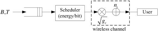
Figure 1: Single-user delay constrained scheduling

Time is indexed in descending order, i.e., $t=T$ is the initial slot, $t=T-1$ is the 2nd slot, $\ldots$, and $t=1$ is the final slot before the deadline; in doing so, $t$ represents the number of remaining slots. The channel state, in power units, is denoted by $g_{t}$. We assume that the channel states $\{g_{t}\}_{t=1}^{T}$ are independently and identically distributed (i.i.d.) and the scheduler has causal knowledge of these channel states (i.e., at time $t$, $g_{T},g_{T-1}\cdots,g_{t}$ are known but $g_{t-1},\cdots,g_{1}$ are unknown). In this context, we refer to this type of scheduler as a causal scheduler. The channel state $g$ is assumed to be a non-degenerate positive continuous random variable.

Assuming unit variance Gaussian additive noise and transmission at capacity, the number of transmitted bits, denoted as $b_{t}$, if $E_{t}$ energy is used is given by $b_{t}=\log_{2}(1+g_{t}E_{t})$. By solving for $E_{t}$ we arrive at a formula for the energy cost in terms of the channel state $g_{t}$, and the number of bits served $b_{t}$:

$$E_{t}(b_{t},g_{t})=\frac{2^{b_{t}}-1}{g_{t}}.$$ (2)

We use $\beta_{t}$ to denote the queue state; i.e., the remaining bits at time slot $t$. Then, $\beta_{t}$ can be calculated recursively as $\beta_{t}=\beta_{t+1}-b_{t+1}$. Given this setup, a scheduler is a sequence of functions $\{b_{t}\}_{t=1}^{T}$ that maps from the remaining bits and the current channel state to the number of bits served, i.e., $b_{t}:\mathbb{R}_{+}\times\mathbb{R}_{++}\to[0,\beta_{t}]$. Then, the optimal energy-efficient scheduler is the set of scheduling functions $\{b_{t}^{\text{opt}}(\cdot,\cdot)\}_{t=1}^{T}$ that minimizes the total expected energy cost (summed over the $T$ slots): i.e.,

$$\min_{b_{T},\cdots,b_{1}}\mathop{\mathbb{missing}}{E}\nolimits\left[\sum_{t=1}^{T}E_{t}(b_{t},g_{t})\right]$$ (3)

subject to $\sum_{t=1}^{T}b_{t}=B$ and $b_{t}\geq 0$ for all $t$.

The optimization in (3) can be formulated sequentially (via dynamic programming) with the remaining bits $\beta_{t}$ as a state variable that summarizes the bit allocation up until the previous time step.

$$b_{t}^{\text{opt}}(\beta_{t},g_{t})=\begin{cases}\arg\min\limits_{0\leq b_{t}\leq\beta_{t}}\left\{E_{t}(b_{t},g_{t})+\mathop{\mathbb{missing}}{E}\nolimits\left[\sum_{s=1}^{t-1}E_{s}(b_{s},g_{s})\Bigg{|}b_{t}\right]\right\},&t=T,\ldots,2,\\ \beta_{1},&t=1.\end{cases}$$ (4)

This is the standard backward iteration: we first determine the optimal action at $t=1$, then find the optimal policy at $t=2$ by taking into account the optimal policy to be used at $t=1$, and so forth. Since $g_{t}$ is known but future channel states $g_{t-1},\ldots,g_{1}$ are unknown, the quantity $E_{t}$ is not random but the future energy costs $E_{t-1},\ldots,E_{1}$ are random. Note also that the optimization (4) should be performed for all possible values of $\beta_{t}$ and $g_{t}$. In other words, deriving the optimal scheduling function $b_{t}^{\text{opt}}$ is equivalent to finding the optimal decision rule for all possible pairs $(\beta_{t},g_{t})$.

III Optimal Scheduling

In this section we attempt to derive the optimal (causal) scheduler using the conventional dynamic programming technique [12]. Unfortunately, an analytic expression is obtained only when $T=2$ (besides the $T=1$ trivial case). For $T>2$, we discuss the difficulty in obtaining an analytic expression. When the scheduler has non-causal knowledge of the future channel states, however, deriving an optimal scheduler is possible; the optimal non-causal scheduler provides useful intuition and is derived in Appendix A.

III-A Optimal Scheduler for $T=2$

In the final time slot ($t=1$), the scheduler is required to transmit all $\beta_{1}$ unserved bits regardless of the channel state $g_{1}$, due to the hard delay constraint. Thus, the energy cost is given by $E_{1}(\beta_{1},g_{1})=(2^{\beta_{1}}-1)/g_{1}$ for all $g_{1}$, and the expected cost to serve $\beta_{1}$ bits in the final slot is $\mathop{\mathbb{missing}}{E}\nolimits_{g_{1}}\left[E_{1}(\beta_{1},g_{1})\right]=\mathop{\mathbb{missing}}{E}\nolimits\left[\frac{1}{g}\right](2^{\beta_{1}}-1)$.

At $t=2$, $g_{2}$ is known but $g_{1}$ is unknown. The scheduler needs to determine $b_{2}$, based on $g_{2}$ and $B$, while balancing the current energy cost (of serving $b_{2}$ bits in the current slot) and the expected future cost (of deferring $B-b_{2}$ bits to the last slot). Thus, the optimum scheduler is the solution to the following minimization:

$$b_{2}^{\text{opt}}(B,g_{2}) = \arg\min_{0\leq b_{2}\leq B}\left(\underbrace{\frac{2^{b_{2}}-1}{g_{2}}}_{\text{current power cost}}+\underbrace{\mathop{\mathbb{missing}}{E}\nolimits_{g_{1}}\left[E_{1}(B-b_{2},g_{1})\right]}_{\text{expected future cost}}\right)$$

$$= \arg\min_{0\leq b_{2}\leq B}\left(\frac{1}{g_{2}}\left(2^{b_{2}}-1\right)+\mathop{\mathbb{missing}}{E}\nolimits\left[\frac{1}{g_{1}}\right]\left(2^{B-b_{2}}-1\right)\right).$$

The objective function in (III-A) is convex, and therefore the minimizer is found by setting the derivative to zero while taking into account the constraints on $b_{2}$:

$$b_{2}^{\text{opt}}(B,g_{2})=\left\langle\frac{1}{2}B+\frac{1}{2}\log_{2}\left(g_{2}\nu_{1}\right)\right\rangle_{0}^{B},$$ (6)

where $\nu_{1}\triangleq\mathop{\mathbb{missing}}{E}\nolimits\left[1/g\right]$ is a constant that depends only on the distribution of the channel state $g$ (see Appendix B for the definition of constants $\nu_{m}$ for $m=1,2,\ldots$). Note that this policy depends only on the unserved bits and the current channel state. This policy is only meaningful when $\nu_{1}$ is finite; this rules out Rayleigh fading, in which case $g$ is exponentially distributed and thus $\mathop{\mathbb{missing}}{E}\nolimits\left[1/g\right]$ is not finite.

Notice that the optimal scheduling function (6) has two additive terms: (a) $\frac{1}{2}B$ corresponds to an equal distribution to time slots $t=1$ and $t=2$, and (b) $\frac{1}{2}\log_{2}\left(g_{2}\nu_{1}\right)$ associated with a measure of the channel quality at $t=2$. That is, if the channel quality $g_{2}$ is bigger than a threshold $1/\nu_{1}$, then more bits are allocated than $\frac{1}{2}B$; if $g_{t}$ is smaller than the threshold then fewer bits are allocated and more bits are deferred to the final slot.

III-B Optimal Scheduler for $T>2$

From (4), the optimization that the scheduler solves at each time step is:

$$J_{t}^{\text{opt}}(\beta_{t},g_{t})=\begin{cases}\min\limits_{0\leq b_{t}\leq\beta_{t}}\left(\frac{2^{b_{t}}-1}{g_{t}}+\bar{J}_{t-1}^{\text{opt}}(\beta_{t}-b_{t})\right),&t\geq 2\\ E_{1}(\beta_{1},g_{1}),&t=1,\end{cases}$$ (7)

where $\bar{J}_{t-1}^{\text{opt}}(\beta)=\mathop{\mathbb{missing}}{E}\nolimits_{g}[J_{t-1}^{\text{opt}}(\beta,g)]$ denotes the cost-to-go function, which is the expected cost to serve $\beta$ bits in $(t-1)$ slots if the optimal control policy is used at each step. This is a one-dimensional convex optimization (pp. 87-88 in [13]) over $b_{t}$ and the optimal solution satisfies

$$b_{t}^{\text{opt}}(\beta,g_{t})=\begin{cases}0,&g_{t}\leq\frac{\ln 2}{(\bar{J}_{t-1}^{\text{opt}})^{\prime}(\beta)},\\ \arg_{b}\left\{\frac{2^{b}}{g_{t}}=\frac{1}{\ln 2}(\bar{J}_{t-1}^{\text{opt}})^{\prime}(\beta-b)\right\},&\frac{\ln 2}{(\bar{J}_{t-1}^{\text{opt}})^{\prime}(\beta)}<g_{t}<\frac{2^{\beta}\ln 2}{(\bar{J}_{t-1}^{\text{opt}})^{\prime}(0)},\\ \beta,&g_{t}\geq\frac{2^{\beta}\ln 2}{(\bar{J}_{t-1}^{\text{opt}})^{\prime}(0)},\end{cases}$$ (8)

assuming $\bar{J}_{t-1}^{\text{opt}}$ is differentiable (pp. 254-255 in [14]), where $\arg_{b}\{\cdot\}$ represents the solution of the argument equation.

When $t=2$, the cost-to-go function $\bar{J}_{1}^{\text{opt}}(\beta)=(2^{\beta}-1)\nu_{1}$ (as well as its derivative) takes on a very simple form and thus (8) can be solved in closed form as in (6). However, the same is not true for $t>2$. Because the optimal policy for $t=2$ is known, the cost-go-to $\bar{J}_{2}^{\text{opt}}(\beta)$ can be written in closed form. The derivative $(\bar{J}_{2}^{\text{opt}})^{\prime}(\beta)$ can also be written in closed form but cannot be analytically inverted; thus, the optimal policy for $t=3$ can only be written in the form of (8) with the second condition given by the following fixed point equation:

$$\frac{2^{b_{3}}}{g_{3}}=2^{\beta-b_{3}}\int_{0}^{\frac{2^{-(\beta-b_{3})}}{\nu_{1}}}\nu_{1}dF(x)+2^{\frac{\beta-b_{3}}{2}}\nu_{1}^{\frac{1}{2}}\int_{\frac{2^{-(\beta-b_{3})}}{\nu_{1}}}^{\frac{2^{\beta-b_{3}}}{\nu_{1}}}\left(\frac{1}{x}\right)^{\frac{1}{2}}dF(x)+2^{\beta-b_{3}}\int_{\frac{2^{\beta-b_{3}}}{\nu_{1}}}^{\infty}\frac{1}{x}dF(x),$$ (9)

where $F$ is the cumulative distribution function of the channel state $g$. As a result, no analytical characterization of $\bar{J}_{3}^{\text{opt}}(\beta)$ is possible, and thus neither $b_{t}^{\text{opt}}(\cdot,\cdot)$ nor $\bar{J}_{t}^{\text{opt}}(\beta)$ can be found in closed form for $t\geq 4$.

Alternately, we can numerically find the optimal scheduler by the discretization method [15]. However, large complexity and memory is required for sufficiently fine discretization. More importantly, this numerical method gives little insight on how the delay constraint and channel state affect the scheduling function.

IV Suboptimal Scheduling Policies

Because the optimal scheduler cannot be written in closed form, it is of interest to develop suboptimal schedulers. The first scheduler is based on the intuition from the optimal $T=2$ policy, and the second is found by solving a relaxed version of the optimization.

IV-A Suboptimal I Scheduler

If we compare the optimal causal scheduler for $T=2$ (Section III-A) to the non-causal scheduler, we can immediately notice that the optimal scheduler determines $b_{2}^{\text{opt}}$ by inverse-waterfilling over channels $g_{2}$ and $1/\nu_{1}$, where the non-causal scheduler inverse waterfills over $g_{2}$ and the actual value of $g_{1}$. This is because of the particularly simple form of the expected future cost. Although the expected future cost does not take on such a simple form for $T>2$, we can get a suboptimal scheduler by simply applying this inverse-waterfilling at every time slot $t$. In other words, at time step $t$, perform inverse-waterfilling over the following $t$ channels:

$$g_{t},\underbrace{\frac{1}{\nu_{1}},\ldots,\frac{1}{\nu_{1}}}_{t-1}$$

to determine how many of the unserved $\beta_{t}$ bits to serve now. We denote this bit allocation policy as $b_{t}^{\rm(I)}$. Since $t-1$ of the $t$ channels are equal, the inverse-waterfilling operation is very simple and the policy is given by

$$b_{t}^{\text{(I)}}(\beta_{t},g_{t})=\left\langle\frac{1}{t}\beta_{t}+\frac{t-1}{t}\log_{2}\frac{g_{t}}{\eta_{t}^{\text{(I)}}}\right\rangle_{0}^{\beta_{t}},$$ (10)

where $\eta_{t}^{\text{(I)}}=1/\nu_{1}$ serves as the channel threshold. Notice that this threshold value depends only on the channel statistics and is constant with respect to $t$.

When the deadline is far away (large $t$), the first term in (10) is negligible and the bit allocation is almost completely dependent on the instantaneous channel quality. As the deadline approaches ($t$ decreases toward $1$), the weight of the channel-dependent second term decreases and the weight of the delay-associated first term increases.

IV-B Suboptimal II Scheduler

The inability to find a general analytic solution to the original optimization (7) is due to complications caused by the constraint $0\leq b_{t}\leq\beta_{t}$ (for each $t$) in the dynamic optimization. However, if we relax this constraint (i.e., allow $b_{t}<0$ and $b_{t}>\beta_{t}$ while maintaining the constraint $\sum_{t=1}^{T}b_{t}=B$) we can derive the optimal policy in closed form.

If we define the function $L_{t}$ as below, then we can show inductively that $L_{t}$ represents the cost-to-go function for the relaxed optimization:

$$L_{t}(\beta_{t})=t2^{\frac{\beta_{t}}{t}}\mathop{\mathbb{missing}}{G}\nolimits(\nu_{t},\nu_{t-1},\ldots,\nu_{1})-t\nu_{1}$$ (11)

where $\nu_{1},\nu_{2},\cdots$ are the fractional moments defined in Appendix B and $\mathop{\mathbb{missing}}{G}\nolimits()$ represents the geometric mean operation defined in Section I. When $t=1$, (11) holds trivially. If we assume (11) holds for $t-1$, then the relaxed optimization for the next time step is given by

$$\min_{b_{t}}\left(\frac{2^{b_{t}}-1}{g_{t}}+L_{t-1}(\beta_{t}-b_{t})\right)$$ (12)

and the solution (i.e., the optimum scheduler for the relaxed problem) is found by setting the derivative of the objective to zero:

$$b_{t}=\frac{1}{t}\beta_{t}+\frac{t-1}{t}\log_{2}\left(g_{t}\mathop{\mathbb{missing}}{G}\nolimits(\nu_{t-1},\ldots,\nu_{1})\right).$$ (13)

By plugging in the optimum value of $b_{t}$ in (13) into (12) and taking expectation with respect to $g_{t}$, we reach (11). By truncating the policy in (13) at $0$ and $\beta_{t}$ we get a policy, referred to as Suboptimal II, for the original (un-relaxed) problem:

$$b_{t}^{\rm(II)}=\left\langle\frac{1}{t}\beta_{t}+\frac{t-1}{t}\log_{2}\frac{g_{t}}{\eta_{t}^{\rm(II)}}\right\rangle_{0}^{\beta_{t}},$$ (14)

where

$$\eta_{t}^{\rm(II)}=\frac{1}{\mathop{\mathbb{missing}}{G}\nolimits\left(\nu_{t-1},\nu_{t-2},\cdots,\nu_{1}\right)}$$ (15)

denotes the threshold that depends only on the statistics not the realizations.

IV-C Remarks on the Suboptimal Schedulers

From (10) and (14), we can see that the two schedulers have a very similar form with the only difference term being the threshold $\eta_{t}$. Notice that both policies simplify to the optimal policy for $t=2$. Based on the policy formulations, this subsection investigates the common and different characteristics of the suboptimal schedulers.

IV-C1 General Framework

The two algorithms thus far considered can be cast into a single framework:

$$b_{t}(\beta_{t},g_{t})=\left\langle\frac{1}{t}\beta_{t}+\frac{t-1}{t}\log_{2}\frac{g_{t}}{\eta_{t}}\right\rangle_{0}^{\beta_{t}},$$ (16)

where $\eta_{t}$ is the channel threshold determined by the individual algorithms. This simple allocation strategy reveals how the delay constraint affects the scheduling algorithms: at time step $t$ serve a fraction $1/t$ of the remaining bits plus/minus a quantity that depends on the strength of the current channel compared to a channel threshold. If the current channel is good (i.e., $g_{t}$ is bigger than the threshold $\eta_{t}$), additional bits are served (up to $\beta_{t}$), while fewer bits are served when the current channel is poorer than the threshold. Furthermore, note that when $t$ is large (i.e., far from the deadline), the first term $\beta_{t}/t$ is very small and the number of bits served is almost completely determined by the current channel conditions. This agrees with intuition that we should make aggressive, almost completely channel dependent (and deadline independent) decisions when the deadline is far away, while we should make more conservative (more deadline dependent, less channel dependent) decisions near the deadline (small $t$).

Using $\log_{2}10\approx 3$ we can rewrite the policy in dB units as:

$$b_{t}(\beta_{t},g_{t})\approx\left\langle\frac{1}{t}\beta_{t}+\left(\frac{t-1}{t}\right)\left(\frac{g_{t}^{\text{dB}}-\eta_{t}^{\text{dB}}}{3}\right)\right\rangle_{0}^{\beta_{t}}.$$ (17)

For large $t$, approximately one bit is allocated for every $3$ dB by which the channel exceeds the threshold.

IV-C2 Channel Thresholds

The difference between the two policies is in the threshold values, which are illustrated in Fig. 2 for a particular channel distribution. The suboptimal I scheduler has a constant threshold $\eta_{t}^{\text{(I)}}=1/\nu_{1}$ for all $t$, whereas Suboptimal II has a threshold that increases with $t$ (by Proposition I). It is intuitive to use a larger threshold when the deadline is far away (large $t$), as the scheduler can be more selective because many different channels remain to be seen before the deadline is reached.

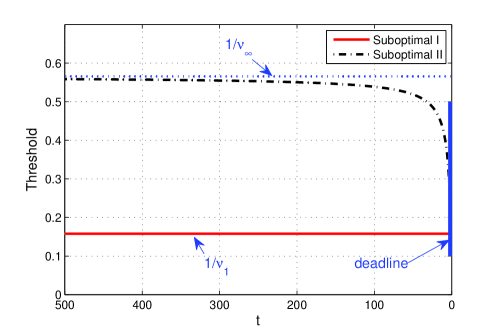
Figure 2: Thresholds $\eta_{t}^{\text{(I)}}$ for the suboptimal I scheduler and $\eta_{t}^{\text{(II)}}$ for the suboptimal II scheduler when the channel state has the truncated exponential with $\gamma_{0}=0.001$.

By using a constant threshold, Suboptimal I is not selective enough and transmits too many bits when the deadline is far away. To see this, consider the average number of bits transmitted in slot $t$ (ignoring truncation):

$$\mathop{\mathbb{missing}}{E}\nolimits_{g_{t}}[b_{t}(\beta_{t},g_{t})]=\mathop{\mathbb{missing}}{E}\nolimits_{g_{t}}\left[\frac{1}{t}\beta_{t}+\frac{t-1}{t}\log_{2}\frac{g_{t}}{\eta_{t}}\right]=\frac{1}{t}\beta_{t}+\frac{t-1}{t}\mathop{\mathbb{missing}}{E}\nolimits\left[\log_{2}\frac{g_{t}}{\eta_{t}}\right].$$ (18)

Because $\eta_{t}^{\text{(I)}}=1/\nu_{1}=1/\mathop{\mathbb{missing}}{E}\nolimits\left[1/g\right]$, by Jensen’s inequality $\mathop{\mathbb{missing}}{E}\nolimits\left[\log_{2}\frac{g_{t}}{\eta_{t}^{\text{(I)}}}\right]=\mathop{\mathbb{missing}}{E}\nolimits\left[\log_{2}g_{t}\right]+\log_{2}\mathop{\mathbb{missing}}{E}\nolimits\left[1/g\right]>0$. Thus, Suboptimal I transmits more than $\frac{B}{T}$ bits on average when scheduling begins, which is in some sense overly aggressive. On the other hand, the quantity $\mathop{\mathbb{missing}}{E}\nolimits_{g_{t}}\left[\log_{2}\left(g_{t}/\eta_{t}^{\text{(II)}}\right)\right]$ decreases as $t$ increases and the limit is given by

$$\lim_{t\to\infty}\mathop{\mathbb{missing}}{E}\nolimits_{g_{t}}\left[\log_{2}\frac{g_{t}}{\eta_{t}^{\text{(II)}}}\right]=0$$ (19)

because of Proposition 1. This implies that the suboptimal II scheduler allocates $B/T$ bits on the average when the deadline is far away and thus, unlike Suboptimal I, is not biased or overly aggressive. Numerical results given later support the fact that Suboptimal II generally performs better than Suboptimal I.

IV-D Equal-bit Scheduler

For comparison purposes, we consider one of the simplest causal schedulers: equal-bit scheduler. This policy allocates $B/T$ bits in each time slot, regardless of channel conditions, i.e.,

$$b_{t}^{\text{eq}}(\beta,g_{t})=\frac{B}{T}=\frac{1}{t}\beta_{t}.$$ (20)

The corresponding expected energy is given by

$$\bar{J}_{t}^{\text{eq}}(\beta)=t(2^{\frac{\beta}{t}}-1)\mathop{\mathbb{missing}}{E}\nolimits\left[\frac{1}{g}\right]=t(2^{\frac{\beta}{t}}-1)\nu_{1}.$$ (21)

Although equal-power scheduling is asymptotically optimal for the dual problem of maximizing rate over $T$ slots when given a finite energy budget in the high power regime [11], it will be seen that equal-bit scheduling is suboptimal even when $B$ is large.

IV-E Inverse Waterfilling Interpretation

If Suboptimal I and II and the equal-bit schedulers are compared to the optimal non-causal policy (inverse waterfilling), one can see that each of the algorithms mimics inverse waterfilling using either the current channel or channel statistics for the future channels, as summarized in Table I.

TABLE I: Waterfilling analogy.

	At each $t$, perform inverse-waterfilling over the following channels
Equal-bit scheduler	$g_{t},\underbrace{g_{t},g_{t},\cdots,g_{t}}_{t-1}$
Suboptimal I scheduler	$g_{t},\underbrace{\frac{1}{\nu_{1}},\frac{1}{\nu_{1}},\cdots,\frac{1}{\nu_{1}}}_{t-1}$
Suboptimal II scheduler	$g_{t},\frac{1}{\nu_{t-1}},\frac{1}{\nu_{t-2}},\cdots,\frac{1}{\nu_{1}}$
Non-causal IWF	$g_{t},g_{t-1},g_{t-2},\cdots,g_{1}$

V Analysis & Numerical Results

In this section, we compare the performance of the optimal, Suboptimal I and II, and equal-bit schedulers. For $T=2$ we are able to quantify the advantage of optimal scheduling relative to equal bit scheduling in two extreme cases, while for $T>2$ we can only consider numerical results.

V-A Asymptotic Analysis for $T=2$

From the optimal scheduling expression for $T=2$ given in (6), we can see that the packet is split over both time slots (i.e., $0<b_{2}<B$) if and only if $2^{-B}/\nu_{1}<g_{2}<2^{B}/\nu_{1}$. As $B\to 0$, the probability of this event goes to zero: if $g_{2}<1/\nu_{1}$ then all bits are deferred to the final slot, while if $g_{2}>1/\nu_{1}$ all bits are served at $t=2$. As a result, the expected energy cost takes on a rather simple form as $B\to 0$ (the derivation is provided in Appendix C):

$$\bar{J}_{2}^{\text{opt}}(B)\cong(2^{B}-1)\mathop{\mathbb{missing}}{E}\nolimits\left[\min\left(\frac{1}{g_{2}},\nu_{1}\right)\right],$$ (22)

where $\cong$ represents equivalence in the limit (i.e., the ratio between both sides converges to $1$ as $B\to 0$). This implies that the corresponding effective channel is $\max(g_{2},1/\nu_{1})$. On the other hand, when $B\to\infty$ the probability of only utilizing one slot goes to zero and the limiting expected cost can be derived. The following theorem quantifies the power advantage of optimal scheduling:

Theorem 1

The energy savings of optimal scheduling with respect to equal bit scheduling in extremes of $B\rightarrow 0$ and $B\rightarrow\infty$ is given by:

$$\lim_{B\to 0}\frac{\bar{J}_{2}^{\text{eq}}(B)}{\bar{J}_{2}^{\text{opt}}(B)} = \frac{\nu_{1}}{\mathop{\mathbb{missing}}{E}\nolimits\left[\min\left(\frac{1}{g},\nu_{1}\right)\right]},$$ (23)

$$\lim_{B\to\infty}\frac{\bar{J}_{2}^{\text{eq}}(B)}{\bar{J}_{2}^{\text{opt}}(B)} = \sqrt{\frac{\nu_{1}}{\nu_{2}}}.$$ (24)

Proof:

See Appendix C. ∎

Table II summarizes typical values of the energy savings (at the extremes of $B\to 0$ and $B\to\infty$) for several fading distributions, as given by Theorem 1. As intuitively expected, the energy advantage is larger for more severe fading distributions. In other words, optimal scheduling is more beneficial in more severe fading environments.

TABLE II: Average energy offsets for $T=2$

	equal-bit vs. optimal causal ($\bar{J}_{2}^{\text{eq}}(B)/\bar{J}_{2}^{\text{opt}}(B)$)
distribution of channel state $g$	$B\to 0$	$B\to\infty$
truncated exponential with $\gamma_{0}=0.1$	1.96 dB	0.44 dB
truncated exponential with $\gamma_{0}=0.01$	3.26 dB	1.04 dB
truncated exponential with $\gamma_{0}=0.001$	4.32 dB	1.68 dB
$1\times 2$ Rayleigh fading ($g\sim\chi^{2}_{4}$)	1.99 dB	0.52 dB
$1\times 3$ Rayleigh fading ($g\sim\chi^{2}_{6}$)	1.37 dB	0.27 dB
$1\times 4$ Rayleigh fading ($g\sim\chi^{2}_{8}$)	1.10 dB	0.18 dB

Figure 3 contains a plot of expected energy versus $B$ for the optimal and equal-bit schedulers as well as a plot of the energy difference between the two schedulers as a function of $B$, for channel state $g$ distributed as a truncated exponential with the threshold $\gamma_{0}=0.001$. The energy advantage is seen to decrease from its $B\rightarrow 0$ advantage of $4.32$ dB to the large $B$ asymptote of $1.68$ dB.

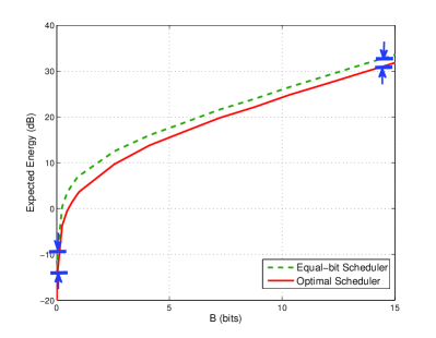
(a) Average total energy

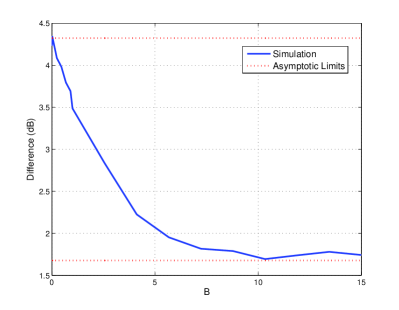
(b) Energy advantage of optimal relative to equal-bit scheduling (difference in dB)

Figure 3: Average total energy consumptions for $T=2$ and average energy offset when $g$ is a truncated exponential variable with threshold $\gamma_{0}=0.001$

V-B Numerical Results for $T>2$

Throughout the simulations, we assume that the channel state $g_{t}$ is a truncated exponential with parameter $\lambda=1$ and threshold $\gamma_{0}=0.001$. The factional moments of this truncated exponential variable can be calculated as:

$$\nu_{m}=\begin{cases}\lambda e^{\lambda\gamma_{0}}\text{E}_{1}(\lambda\gamma_{0}),&m=1,\\ \lambda\left[e^{\lambda\gamma_{0}}\Gamma\left(\frac{m-1}{m},\lambda\gamma_{0}\right)\right]^{m},&m>1,\end{cases}$$

where ${\rm E_{1}}(\cdot)$ and $\Gamma(\cdot,\cdot)$ denote the exponential integral and the incomplete gamma function, respectively, and its limit is given by $\nu_{\infty}=\frac{1}{\gamma_{0}}e^{-e^{\lambda\gamma_{0}}\text{E}_{1}(\lambda\gamma_{0})}$.

Figures 4a and 4b compare the energy consumption of the four different algorithms (equal-bit, Suboptimal I and II, optimal causal) for $T=5$ and $T=50$, in which the optimal scheduler is calculated by numerical methods. The $x$-axis denotes the total number of bits $B$ transmitted in $T$ time slots, and thus $B/T$ can be thought of as the average bits per channel use. The $y$-axis denotes the average total energy cost $\bar{J}_{T}^{\text{eq}}$, $\bar{J}_{T}^{\text{(I)}}$, $\bar{J}_{T}^{\text{(II)}}$, and $\bar{J}_{T}^{\text{opt}}$.

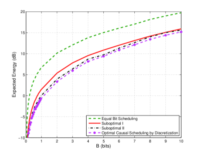
(a) $T=5$

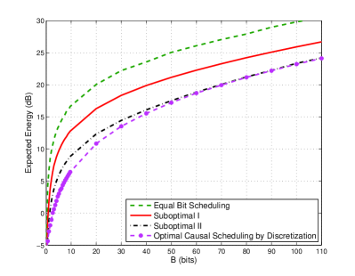
(b) $T=50$

Figure 4: Average total energy consumption for $T=5$ and $T=50$

From Fig. 4a we see that both Suboptimal I and II perform nearly as well as the optimal scheduler, although Suboptimal II performs better than I. There are significant differences between the equal-bit and optimal schedulers, which is to be expected given the time diversity available over the five time slots. In Fig. 4b we see even larger differences between equal-bit and optimal causal, which can be explained by the even larger degree of time diversity ($T=50$). Furthermore, Suboptimal II significantly outperforms Suboptimal I for $T=50$ due to the over-aggressive nature of Suboptimal I. Suboptimal II performs nearly as well as the optimal scheduler when $B$ is approximately $50$ or larger (i.e., $B/T\geq 1$), but is sub-optimal for smaller values of $B$.

Figure 5 shows the expected bit allocation $\mathop{\mathbb{missing}}{E}\nolimits[b_{t}]$ for the different algorithms for $T=10$ slots when $B$ is large ($B=50$, upper) and small ($B=2$, lower). While the optimal causal scheduling policy allocates roughly an equal number of bits (averaged across different realizations, and not for each particular realization) to each of the slots, Suboptimal I is immediately seen to allocate too many bits (on average) to early time slots which agrees with our earlier claim that this algorithm is often overly-aggressive as explained in Section IV-C2. For $B=50$ the bit allocation of Suboptimal II is very similar to that of the optimal policy. However, for $B=2$ Suboptimal II is also overly-aggressive as compared to the optimal. We suspect that the performance of Suboptimal II could be further improved by performing some heuristic modifications to the algorithm, but this is beyond the scope of the paper and is left to future work.

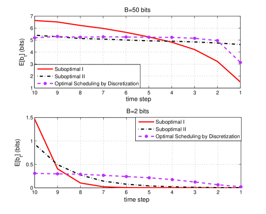
Figure 5: Bit allocation profiles for $T=10$ when $B=50$ (upper) and $B=2$ (lower)

To summarize, the numerical results indicate that (a) Suboptimal II is nearly optimal for moderate to large values of $B$, (b) Suboptimal II outperforms Suboptimal I, and (c) neither suboptimal algorithm is near optimal for small values of $B$. In the next section, we will consider a policy that performs close to the optimal when $B$ is small.

VI One-shot Allocation

In some settings it may be undesirable to split the packet across multiple time slots, e.g., because there is a large overhead associated with each slot used for transmission. In this scenario we may wish to find only one time slot among the $T$ slots for the transmission of $B$ bits; i.e., the action $b_{t}$ can be either $0$ or $B$.

The dynamic program in this setting can be written as

$$J_{1}(B) = \frac{2^{B}-1}{g_{1}},$$ (25)

$$J_{t}(B) = \min\left\{\frac{2^{B}-1}{g_{t}},\mathop{\mathbb{missing}}{E}\nolimits[J_{t-1}(B)]\right\},\qquad t=2,\cdots,T,$$ (26)

which is precisely an optimal stopping problem [12]. Thus, a threshold policy is optimal: allocate all $B$ bits at the first slot $t$ such that $g_{t}>1/\omega_{t}$, where $1/\omega_{t}$ is the threshold. That is,

$$b_{t}=\begin{cases}B,&t=\max\left\{s:g_{s}>1/\omega_{s}\right\},\\ 0,&\text{elsewhere}.\end{cases}$$ (27)

At $t=1$ a packet must be served and thus $\omega_{1}$ is infinite. Because the expected cost-to-go decreases as $t$ increases, the threshold also decreases with $t$. In Appendix D we show the thresholds are given by the following recursive formula.

$$\omega_{t}=\begin{cases}\mathop{\mathbb{missing}}{E}\nolimits\left[\frac{1}{g}\right],&t=2,\\ \mathop{\mathbb{missing}}{E}\nolimits\left[\frac{1}{g}\Big{|}\frac{1}{g_{t}}<\omega_{t-1}\right]\Pr\left\{\frac{1}{g_{t}}<\omega_{t-1}\right\}+\omega_{t-1}\Pr\left\{\frac{1}{g_{t}}\geq\omega_{t-1}\right\},&t=3,\cdots,T.\end{cases}$$ (28)

Notice that the threshold $1/\omega_{t}$ depends only on the channel statistics and does not depend on $B$.

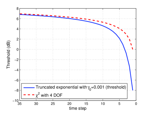
Figure 6: Thresholds for the one-shot allocation

Figure 6 illustrates the thresholds for the truncated exponential $g$ (with $\lambda=1$ and $\gamma_{0}=0.001$) and the chi-squared $g$ (with 4 degrees of freedom). Figure 7 illustrates the energy usage (normalized by $T$) of the optimal one-shot allocation policy and the multiple slot policies. The $B/T=0.1$ and $B/T=1$ curves illustrate performance for relatively small and large values of $B$, respectively. When $B$ is small, the energy of the one-shot allocation is nearly the same as the optimal policy that allows for multiple slots to be used. However, this one-shot allocation is not appropriate when $B$ is relatively large because the required energy of the one-shot policy grows exponentially with $B$.

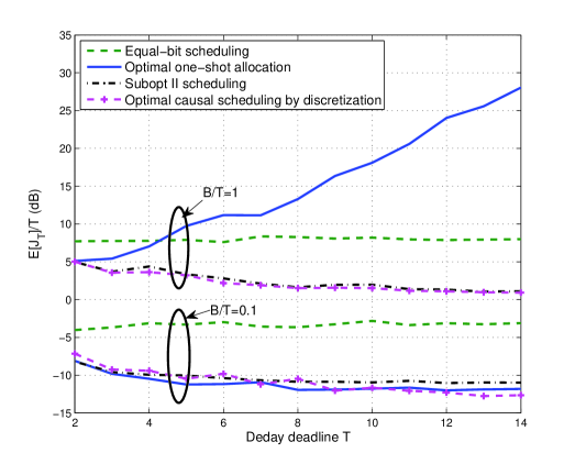
Figure 7: Performance of the optimal one-shot allocation compared with multi-slot allocation algorithms

VII Conclusion

In this paper we considered the problem of bit/energy allocation for transmission of a finite number of bits over a finite delay horizon, assuming perfect instantaneous channel state information is available to the transmitter and that the energy and rate are related by the Shannon-type (exponential) function. We derived the optimal scheduling policy when the deadline spans two time slots, and derived two near-optimal policies for general deadlines. The proposed schedulers have a simple and intuitive form that gives insight into the optimal balance between channel-awareness (i.e., opportunism) and deadline-awareness in a delay-limited setting. We also considered the same problem under the additional constraint that only a single of the available time slots can be used, and in this case found the optimal threshold-based policy. Based upon the policy constructions and the numerical results, we observed that the suboptimal II scheduler is near-optimal for large/moderate values of $B$ while the one-shot policy is near-optimal for small values of $B$.

Given the increasing volume of delay-limited traffic over packet-switched wireless networks (e.g., VoIP or multimedia transmission in 3G systems), we expect problems of this sort to become increasingly important. Of course, the problem considered here represents only a particular instance of the rich space of delay-limited scheduling problems. Interesting extensions include consideration of discrete code rates, peak power constraints, and multi-user issues, and we hope this work provides useful insight for some of these other formulations.

Appendix A Non-causal Scheduling

If the channel states are known non-causally, i.e., $g_{T},\ldots,g_{1}$ are known at $t=T$, the optimal scheduling/allocation is determined by waterfilling because each time slot serves as a parallel channel. While conventional waterfilling maximizes rate subject to a power constraint, this is the dual of minimizing power/energy subject to a rate/bit constraint and is referred to as inverse-waterfilling (IWF):

$$J_{T}^{\text{IWF}}(B,\{g_{t}\}_{t=1}^{T})=\min_{b_{T},\cdots,b_{1}}\sum_{t=1}^{T}\frac{2^{b_{t}}-1}{g_{t}},$$ (29)

subject to $\sum_{t=1}^{T}b_{t}=B$ and $b_{t}\geq 0$. This is a convex optimization problem and can be easily solved using the standard Lagrangian method:

$$b_{t}^{\text{IWF}}=\left\langle\log_{2}\left(\frac{g_{t}}{g_{\text{th}}}\right)\right\rangle_{0}^{\infty},$$ (30)

where $g_{\text{th}}$ is the solution to $\sum_{i=1}^{T}\left\langle\log_{2}\left(\frac{g_{i}}{g_{\text{th}}}\right)\right\rangle_{0}^{\infty}=B$. A time slot $t$ is called utilized if a positive bit is scheduled at $t$, i.e., $b_{t}>0$ or equivalently $g_{t}>g_{\text{th}}$. With algebraic manipulations, we can express this IWF policy in (30) sequentially like other causal scheduling policies as

$$b_{t}^{\text{IWF}}(\beta_{t},g_{t})=\frac{1}{t^{\prime}}\beta_{t}+\frac{t^{\prime}-1}{t^{\prime}}\log_{2}\frac{g_{t}}{\eta_{t}^{\text{IWF}}},\qquad\text{if}\;\;g_{t}>g_{\text{th}},$$ (31)

otherwise $b_{t}^{\text{IWF}}(\beta_{t},g_{t})=0$, where $t^{\prime}=\sum_{i=1}^{t}1_{\{g_{i}\geq g_{\rm th}\}}$ and $\eta_{t}^{\text{IWF}}=\left(\prod\limits_{i=1}^{t-1}g_{i}^{1_{\{g_{i}>g_{\text{th}}\}}}\right)^{1/(t^{\prime}-1)}$. Notice that $g_{t-1},\cdots,g_{1}$ are relatively future quantities at slot $t$.

Like causal scheduling, the bit allocation process is described in two stages: first the remaining bits are divided equally amongst the active slots and then bits are added/subtracted depending on the channel state.

Appendix B Channel Characterization by Fractional Moments

We characterize the statistics of the channel states by using the fractional moments of the inverse of the channel states $g$. We define the following quantity for $m=1,2,\ldots$,

$$\nu_{m}=\left(\mathop{\mathbb{missing}}{E}\nolimits\left[\left(\frac{1}{g}\right)^{\frac{1}{m}}\right]\right)^{m}.$$ (32)

Then, the properties of these quantities are summarized as follows:

Proposition 1

The channel statistics defined according to (32) for a non-degenerate positive random variable have the following properties:

1. the sequence $\{\nu_{m}\}$ is strictly decreasing and the limit exists (denote the limit as $\nu_{\infty}$),

2. the sequence $\{(\nu_{m}\nu_{m-1}\cdots\nu_{1})^{1/m}\}$ is also strictly decreasing and its limit is also $\nu_{\infty}$.

Proof:

1. First, we show the sequence $\{\nu_{m}\}$ is monotonically decreasing. Let $Y=1/g$ and $f_{Y}(y)$ be the pdf of $Y$. By the Hölder’s inequality [16],

   $$\mathop{\mathbb{missing}}{E}\nolimits\left[Y^{\frac{1}{m+1}}\right] = \int_{0}^{\infty}y^{\frac{1}{m+1}}f_{Y}(y)dy$$

   $$= \int_{0}^{\infty}\left(y^{\frac{1}{m}}f_{Y}(y)\right)^{\frac{m}{m+1}}\left(f_{Y}(y)\right)^{\frac{1}{m+1}}dy$$

   $$< \left(\int_{0}^{\infty}y^{\frac{1}{m}}f_{Y}(y)dy\right)^{\frac{m}{m+1}}\left(\int_{0}^{\infty}f_{Y}(y)dy\right)^{\frac{1}{m+1}}=\left(\mathop{\mathbb{missing}}{E}\nolimits[Y^{\frac{1}{m}}]\right)^{\frac{m}{m+1}}.$$

   The strict inequality is due to the fact that $Y$ is not a point-mass density. Raising both sides to the power $(m+1)$ gives $\nu_{m+1}<\nu_{m}$.

   Second, we show convergence of the sequence. Let $\phi_{m}(y)=y^{\frac{1}{m}}$ for $y>0$ and $\psi(y)=1+y$ for $y>0$. Then, it is clear that $\lim_{m\to\infty}\phi_{m}(y)=1$ for all $y>0$, and $0<\phi_{m}(y)\leq\psi(y)$ for all $y>0$. Additionally, $\int_{0}^{\infty}\psi(y)f_{Y}(y)dy<\infty$. By the dominated convergence theorem [16], we have

   $$\lim_{m\to\infty}\mathop{\mathbb{missing}}{E}\nolimits[Y^{\frac{1}{m}}]=\lim_{m\to\infty}\int_{0}^{\infty}\phi_{m}(y)f_{Y}(y)dy=\int_{0}^{\infty}1\cdot f_{Y}(y)dy=1.$$

   Let $x$ be a positive real number. By the continuity of the logarithmic function, we have $\lim_{x\to 0}\ln\mathop{\mathbb{missing}}{E}\nolimits[Y^{x}]=0$. By L’Hospital rule,

   $$\lim_{x\to 0}\frac{\ln\mathop{\mathbb{missing}}{E}\nolimits[Y^{x}]}{x}=\lim_{x\to 0}\frac{\mathop{\mathbb{missing}}{E}\nolimits[Y^{x}\ln Y]}{\mathop{\mathbb{missing}}{E}\nolimits[Y^{x}]}=\mathop{\mathbb{missing}}{E}\nolimits[\ln Y]$$

   since $\lim_{x\to 0}\mathop{\mathbb{missing}}{E}\nolimits[Y^{x}]=1$ and $\lim_{x\to 0}\mathop{\mathbb{missing}}{E}\nolimits[Y^{x}\ln Y]=\mathop{\mathbb{missing}}{E}\nolimits[\ln Y]$ (due to the dominated convergence theorem). By the continuity of the exponential function, $\lim_{x\to 0}e^{\frac{1}{x}\ln\mathop{\mathbb{missing}}{E}\nolimits[Y^{x}]}=e^{\mathop{\mathbb{missing}}{E}\nolimits[\ln Y]}$. Since the above limit exists and $x$ is in the superset of integers, we have the result.

2. The monotonicity of the sequence $\{(\nu_{m}\nu_{m-1}\cdots\nu_{1})^{1/m}\}$ follows immediately from the monotonicity of the sequence $\{\nu_{m}\}$ and its positivity.

   By the property of the exponential function, we have $\left(\nu_{m}\nu_{m-1}\cdots\nu_{1}\right)^{\frac{1}{m}}=e^{\frac{1}{m}\ln(\nu_{m}\nu_{m-1}\cdots\nu_{1})}=e^{\frac{1}{m}\sum_{n=1}^{m}\ln\nu_{n}}$. Since $\lim_{m\to\infty}\nu_{m}=\nu_{\infty}$ and $\log$ is continuous, $\lim_{m\to\infty}\ln\nu_{m}=\ln\nu_{\infty}$. By Cesáro mean,

   $$\lim_{m\to\infty}\frac{1}{m}\sum_{n=1}^{m}\ln\nu_{n}=\ln\nu_{\infty}.$$

   From the continuity of the exponential function, we have the result.

∎

Notice that $\nu_{1}$ and $\nu_{\infty}$ represent the arithmetic mean and the geometric mean of random variable $1/g$, respectively. All other values in the sequence $\{\nu_{m}\}$ lie between these two means.

Appendix C Proof of Theorem 1

For simple derivation, we work in units of nats rather than bits. From (6), the energy cost can be derived as

$$J_{2}^{\text{opt}}(g_{2},B)=\begin{cases}(e^{B}-1)\nu_{1},&g_{2}\leq\frac{e^{-B}}{\nu_{1}},\\ 2e^{\frac{B}{2}}\left(\frac{1}{g_{2}}\nu_{1}\right)^{1/2}-\frac{1}{g_{2}}-\nu_{1},&\frac{e^{-B}}{\nu_{1}}<g_{2}<\frac{e^{B}}{\nu_{1}},\\ \frac{e^{B}-1}{g_{2}},&g_{2}\geq\frac{e^{B}}{\nu_{1}}.\end{cases}$$ (33)

Thus,

$$\bar{J}_{2}^{\text{opt}}(B) = \mathop{\mathbb{missing}}{E}\nolimits_{g_{2}}\left[J_{2}^{\text{opt}}(g_{2},B)\right]$$

$$= \int_{0}^{\frac{e^{-B}}{\nu_{1}}}(e^{B}-1)\nu_{1}dF(x)+\int_{\frac{e^{-B}}{\nu_{1}}}^{\frac{e^{B}}{\nu_{1}}}\left[2e^{\frac{B}{2}}\left(\frac{1}{x}\nu_{1}\right)^{1/2}-\frac{1}{x}-\nu_{1}\right]dF(x)$$

$$\qquad\qquad+\int_{\frac{e^{B}}{\nu_{1}}}^{\infty}\frac{e^{B}-1}{x}dF(x),$$

where $F$ is the cumulative distribution function (CDF) of the channel state $g$.

By the limit rules,

$$\lim_{B\to 0}\frac{\bar{J}_{2}^{\text{opt}}(B)}{e^{B}-1} = \lim_{B\to 0}\frac{\left\{\int_{0}^{\frac{e^{-B}}{\nu_{1}}}(e^{B}-1)\nu_{1}dF(x)+\int_{\frac{e^{B}}{\nu_{1}}}^{\infty}\frac{e^{B}-1}{x}dF(x)\right\}}{e^{B}-1}$$ (35)

$$= \lim_{B\to 0}\frac{\int_{0}^{\infty}(e^{B}-1)\min\left(\frac{1}{x},\nu_{1}\right)dF(x)}{e^{B}-1}$$

$$= \mathop{\mathbb{missing}}{E}\nolimits\left[\min\left(\frac{1}{g},\nu_{1}\right)\right]$$

and

$$\lim_{B\to 0}\frac{e^{B}-1}{2(e^{B/2}-1)}=1.$$ (36)

With (21), we obtain (23). Likewise,

$$\lim_{B\to\infty}\frac{\bar{J}_{2}^{\text{opt}}(B)}{2e^{\frac{B}{2}}(\nu_{2}\nu_{1})^{1/2}} = \lim_{B\to\infty}\frac{\int_{\frac{e^{-B}}{\nu_{1}}}^{\frac{e^{B}}{\nu_{1}}}\left[2e^{\frac{B}{2}}\left(\frac{1}{x}\nu_{1}\right)^{1/2}-\frac{1}{x}-\nu_{1}\right]dF(x)}{2e^{\frac{B}{2}}(\nu_{2}\nu_{1})^{1/2}}$$ (37)

$$= \lim_{B\to\infty}\frac{2e^{\frac{B}{2}}\left(\nu_{2}\nu_{1}\right)^{1/2}-2\nu_{1}}{2e^{\frac{B}{2}}(\nu_{2}\nu_{1})^{1/2}}=1$$

and

$$\lim_{B\to\infty}\frac{\bar{J}_{2}^{\text{eq}}(B)}{2e^{\frac{B}{2}}\nu_{1}}=1$$ (38)

Thus, we have shown (24).

Appendix D Derivation of (28)

From (26) the threshold $\omega_{t}$ is related to the expected cost-to-go by $\omega_{t}=\frac{1}{2^{B}-1}\mathop{\mathbb{missing}}{E}\nolimits[J_{t-1}(B)]$. The one-step cost-to-go is $\mathop{\mathbb{missing}}{E}\nolimits[J_{1}(B)]=(2^{B}-1)\mathop{\mathbb{missing}}{E}\nolimits\left[\frac{1}{g}\right]$ and therefore $\omega_{2}=\mathop{\mathbb{missing}}{E}\nolimits\left[\frac{1}{g}\right]$. For $t>2$, we expand the cost-to-go in terms of $\omega_{t-1}$ to give:

$$\omega_{t} = \frac{1}{2^{B}-1}\mathop{\mathbb{missing}}{E}\nolimits[J_{t-1}(B)]$$

$$= \frac{1}{2^{B}-1}\Bigg{(}\mathop{\mathbb{missing}}{E}\nolimits\left[\frac{2^{B}-1}{g_{t-1}}\Bigg{|}\frac{1}{g_{t-1}}<\omega_{t-1}\right]\Pr\left\{\frac{1}{g_{t-1}}<\omega_{t-1}\right\}+$$

$$\hskip 80.0pt\mathop{\mathbb{missing}}{E}\nolimits\left[\mathop{\mathbb{missing}}{E}\nolimits[J_{t-2}(B)]\Bigg{|}\frac{1}{g_{t-1}}<\omega_{t-1}\right]\Pr\left\{\frac{1}{g_{t-1}}\geq\omega_{t-1}\right\}\Bigg{)}$$

By substituting $\mathop{\mathbb{missing}}{E}\nolimits[J_{t-2}(B)]=(2^{B}-1)\omega_{t-1}$, we have the result.

References

- [1] R. A. Berry and R. G. Gallager, “Communication over fading channels with delay constraints,” IEEE Trans. Inf. Theory, vol. 48, no. 5, pp. 1135–1149, May. 2002.
- [2] D. Rajan, A. Sabharwal, and B. Aazhang, “Delay-bounded packet scheduling of bursty traffic over wireless channels,” IEEE Trans. Inf. Theory, vol. 50, no. 1, pp. 125–144, Jan. 2004.
- [3] B. E. Collins and R. L. Cruz, “Transmission policies for time varying channels with average delay constraints,” in Proc. 1999 Allerton Conf. on Commun., Control, & Comp., Monticello, IL, 1999.
- [4] B. Prabhakar, E. Uysal-Biyikoglu, and A. E. Gamal, “Energy-efficient transmission over a wireless link via lazy packet scheduling,” in Proc. IEEE INFOCOM, Anchorage, AK, Apr. 2001, pp. 386–394.
- [5] E. Uysal-Biyikoglu and A. E. Gamel, “On adaptive transmission for energy efficient in wireless data networks,” IEEE Trans. Inf. Theory, vol. 50, 2004.
- [6] M. J. Neely, “Optimal energy and delay tradeoffs for multiuser wireless downlinks,” IEEE Trans. Inf. Theory, vol. 53, no. 9, pp. 3095–3113, Sep. 2007.
- [7] W. Chen, M. J. Neely, and U. Mitra, “Energy efficient scheduling with individual packet delay constraints: Offline and online results,” in Proc. IEEE INFOCOM, Anchorage, AK, May 2007, pp. 1136–1144.
- [8] ——, “Energy efficient scheduling with individual delay constraints over a fading channel,” in Proc. WiOpt, 2007.
- [9] A. Fu, E. Modiano, and J. N. Tsitsiklis, “Optimal transmission scheduling over a fading channel with energy and deadline constraints,” IEEE Trans. Wireless Commun., vol. 5, no. 3, pp. 630–641, Mar. 2006.
- [10] M. Zafer and E. Modiano, “Delay constrained energy efficient data transmission over a wireless fading channel,” in Workshop on Inf. Theory and Appl., La Jolla, CA, Jan./Feb. 2007, pp. 289–298.
- [11] R. Negi and J. M. Cioffi, “Delay-constrained capacity with causal feedback,” IEEE Trans. Inf. Theory, vol. 48, no. 9, pp. 2478–2494, Sep. 2002.
- [12] D. P. Bertsekas, Dynamic Programming and Optimal Control, 3rd ed. Mass.: Athena Scientific, 2005, vol. 1.
- [13] S. Boyd and L. Vandenberghe, Convex Optimization. Cambridge, UK: Cambridge Univ. Press, 2004.
- [14] R. T. Rockafellar, Convex Analysis. Princeton Univ. Press, 1970.
- [15] D. P. Bertsekas, “Convergence of discretization procedures in dynamic programming,” IEEE Trans. Automat. Contr., vol. AC-20, no. 3, pp. 415–419, Jun. 1975.
- [16] W. Rudin, Real and Complex Analysis, 3rd ed. McGraw-Hill, 1987.