A Fortran 90 program to solve the Hartree-Fock equations for interacting spin-$\frac{1}{2}$ Fermions confined in Harmonic potentials

Abstract

A set of weakly interacting spin-$\frac{1}{2}$ Fermions, confined by a harmonic oscillator potential, and interacting with each other via a contact potential, is a model system which closely represents the physics of a dilute gas of two-component Fermionic atoms confined in a magneto-optic trap. In the present work, our aim is to present a Fortran 90 computer program which, using a basis set expansion technique, solves the Hartree-Fock (HF) equations for spin-$\frac{1}{2}$ Fermions confined by a three-dimensional harmonic oscillator potential, and interacting with each other via pair-wise delta-function potentials. Additionally, the program can also account for those anharmonic potentials which can be expressed as a polynomial in the position operators $x,$ $y$, and $z$. Both the restricted-HF (RHF), and the unrestricted-HF (UHF) equations can be solved for a given number of Fermions, with either repulsive or attractive interactions among them. The option of UHF solutions for such systems also allows us to study possible magnetic properties of the physics of two-component confined atomic Fermi gases, with imbalanced populations. Using our code we also demonstrate that such a system exhibits shell structure, and follows Hund’s rule.

Program Summary
Title of program: trap.x
Catalogue Identifier:
Program summary URL:
Program obtainable from: CPC Program Library, Queen’s University of Belfast, N. Ireland
Distribution format: tar.gz
Computers : PC’s/Linux, Sun Ultra 10/Solaris, HP Alpha/Tru64, IBM/AIX
Programming language used: mostly Fortran 90
Number of bytes in distributed program, including test data, etc.: size of the gzipped tar file 371074 bytes
Card punching code: ASCII
Nature of physical problem: The simplest description of a spin $\frac{1}{2}$ trapped system at the mean field level is given by the Hartree-Fock method. This program presents an efficient approach of solving these equations. Additionally, this program can solve for time-independent Gross-Pitaevskii and Hartree-Fock equations for bosonic atoms confined in a harmonic trap. Thus the combined program can handle mean-field equations for both the fermi and the bose particles.
Method of Solution: The solutions of the Hartree-Fock equation corresponding to the fermi systems in atomic traps are expanded as linear combinations of simple-harmonic oscillator eigenfunctions. Thus, the Hartree-Fock equations which comprises of a set of nonlinear integro-differential equation, is transformed into a matrix eigenvalue problem. Thereby, its solutions are obtained in a self-consistent manner, using methods of computational linear algebra.
Unusual features of the program: None

1 Introduction

Over the last several years, there has been an enormous amount of interest in the physics of dilute Fermi gases confined in magneto-optic traps[1, 2, 3, 4, 5]. With the possibility of tuning the atomic scattering lengths from the repulsive regime to an attractive one using the Feshbach resonance technique, there has been considerable experimental activity in looking for phenomenon such as superfluidity, and other phase transitions in these systems[1, 2]. This has led to equally vigorous theoretical activity starting from the studies of so-called BEC-BCS crossover physics[3], search for shell-structure in these systems[4], to the study of more complex phases[5]. As far as the spin of the fermions is concerned, most attention has been given to the cases of two-component gases which can be mapped to a system of spin-$\frac{1}{2}$ atoms[3, 4]. Therefore, in our opinion, a quantum-mechanical study of spin-$\frac{1}{2}$ fermions moving in a harmonic oscillator potential, and interacting via a pair-wise delta function potential, can help us achieve insights into the physics of dilute gases of trapped fermionic atoms.

With the aforesaid aims in mind, the purpose of this paper is to describe a Fortran 90 computer program developed by us which can solve the Hartree-Fock equations for spin-$\frac{1}{2}$ fermions moving in a three-dimensional (3D) harmonic oscillator potential, and interacting via delta-function potential. A basis set approach has been utilized in the program, in which the single-particle orbitals are expanded as a linear combination of the 3D simple harmonic oscillator basis functions, expressed in terms of Cartesian coordinates. The program can solve both the restricted-Hartree-Fock (RHF), and the unrestricted Hartree-Fock (UHF) equations, the latter being useful for fermi gases with imbalanced populations. We would like to clarify, that as far as the applications of this approach to dilute Fermi gases is concerned, at present it is not possible to reach the thermodynamic limit of very large $N$, where $N$ is the total number of atoms in the trap. However, we believe that by solving the HF equations for a few tens of atoms, one may be able to achieve insights into the microscopic aspects such as the nature of pairing in such systems. This program is an extension of an earlier program developed in our group, aimed at solving the time-independent Gross-Pitaevskii equation (GPE) for harmonically trapped Bose gases[6]. Thus the combined total program accompanying this paper can now solve for both Bose and Fermi systems, confined to move in a harmonic oscillator potential, with mutual interactions of the delta-function form. As with our earlier boson program, because of the use of a Cartesian harmonic oscillator basis set, the new program can handle trap geometries ranging from spherical to completely anisotropic, and it can also account for those trap anharmonicities which can be expressed as polynomials in the Cartesian coordinates. The nature of interparticle interactions, i.e., whether they are attractive or repulsive, also imposes no restrictions on the program. We note that Yu et al.[4] have recently described a Hartree-Fock approach for dealing with two-component fermions confined in harmonic traps with spherical symmetry, employing a finite-difference-based numerical approach. However, we would like to emphasize that, as mentioned earlier, our approach is more general in that it is not restricted to any particular trap symmetry. Apart from describing the program, we also present and discuss several of its applications. With the aim of exploring the shell-structure in trapped fermionic atoms, using our UHF approach we compute the addition energy for spherically trapped fermions for various particle numbers, and obtain results consistent with a shell-structure and Hund’s rule.

The remainder of the paper is organized as follows. In the next section we discuss the basic theoretical aspects of our approach. In section 3, we briefly describe the most important subroutines that comprise the new enlarged program. Section 4 contains a brief note on how to install the program and prepare the input files. In section 5 we discuss results of several example runs of our program for different geometries. In the same section, we also discuss issues related to the convergence of the procedure. Finally, in section 6, we end this paper with a few concluding remarks.

2 Theory

We consider a system of $N$ identical spin-$\frac{1}{2}$ particles of mass $m$, moving in a 3D potential with harmonic and anharmonic terms, interacting with each other via a pair-wise delta function potential. The Hamiltonian for such a system can be written as

$$H=\sum_{i=1}^{N}h({\bf r}_{i})+g\sum_{i>j}^{N}\delta({\bf r}_{i}-{\bf r}_{j}),$$ (1)

where ${\bf r}_{i}$ represents the position vector of $i-$th particle, $g$ represents the strength of the delta-function interaction, and $h({\bf r}_{i})$ denotes the one-particle terms of the Hamiltonian

$$h({\bf r}_{i})=-\frac{\hbar^{2}}{2m}\mathbf{\nabla}_{i}^{2}+\frac{1}{2}m(\omega_{x}^{2}x_{i}^{2}+\omega_{y}^{2}y_{i}^{2}+\omega_{z}^{2}z_{i}^{2})+V^{anh}(x_{i},y_{i},z_{i}),$$ (2)

where $\omega_{x}$, $\omega_{y}$ and $\omega_{z}$ are the angular frequencies of the external harmonic potential in the $x$, $y$ and $z$ directions, respectively, and $V^{anh}(x_{i},y_{i},z_{i})$ represents any anharmonicity in the potential. In order to parametrize the strength of the delta-function interactions, we use the formula $g=\frac{4\pi\hbar^{2}a}{m}$ in our program, where $a$ is the $s$-wave scattering length for the atoms. Next we will obtain the RHF and the UHF equations for the system.

Assuming that $N=2n$, and that the many-particle wave function of the system can be represented by a single closed-shell Slater determinant, the RHF equations for the $n$ doubly occupied orbitals $\{\psi_{i}({\bf r}),\>i=1,\ldots,n\}$ of the system are obtained to be[7]

$$(h+g\sum_{j=1}^{n}|\psi_{j}({\bf r})|^{2})\psi_{i}({\bf r})=\epsilon_{i}\psi_{i}({\bf r}).$$ (3)

Similarly, for a system with $n_{1}$ up-spin ($\alpha$) fermions, and $n_{2}$ down-spin ($\beta$) fermions $(n_{1}+n_{2}=N)$, the UHF equations for the up-spin orbitals can be written as[7]

$$(h+g\sum_{j=1}^{n_{2}}|\psi_{j}^{(\beta)}({\bf r})|^{2})\psi_{i}^{(\alpha)}({\bf r})=\epsilon_{i}\psi_{i}^{(\alpha)}({\bf r}),$$ (4)

where $\{\psi_{i}^{(\alpha)}({\bf r}),\>i=1,\ldots,n_{1}\}$ and $\{\psi_{j}^{(\beta)}({\bf r}),\>j=1,\ldots,n_{2}\}$, represent the occupied orbitals corresponding to the up and the down spins, respectively. Similar to the the UHF equations for the down-spin orbitals can be deduced easily from Eq. (4). As in our earlier work on the bosonic systems[6], we adopt a basis-set approach and expand the HF orbitals in terms of the 3D Harmonic oscillator basis functions. This approach is fairly standard, and is well-known as the Hartree-Fock-Roothan procedure in the quantum chemistry community[7]. Thus, for the RHF case, the orbitals are expressed as

$$\psi_{i}({\bf r})=\sum_{j=1}^{N_{basis}}C_{ji}\Phi_{n_{xj},n_{yj},n_{zj}}({\bf r})=\sum_{j=1}^{N_{basis}}C_{ji}\phi_{n_{xj}}(x)\phi_{n_{yj}}(y)\phi_{n_{zj}}(z),$$ (5)

where $C_{ji}$ represents the coefficient corresponding to the $j$-th 3D harmonic oscillator basis function $\Phi_{n_{xj},n_{yj},n_{zj}}({\bf r})$, in the expansion of the $i$-th occupied orbital $\psi_{i}({\bf r})$, and $N_{basis}$ is the total number of basis functions used. Note that $\Phi_{n_{xj},n_{yj},n_{zj}}({\bf r})$ is itself a product of three linear harmonic oscillator eigenfunctions of quantum numbers $n_{xj},$ $n_{yj}$, and $n_{zj}$. Therefore, a set of functions $\Phi_{n_{xj},n_{yj},n_{zj}}({\bf r})$, for different values of $n_{xj},$ $n_{yj}$, and $n_{zj}$, will constitute an orthonormal basis set, leading to an overlap matrix which is identity matrix. For the UHF case, the corresponding expansion for up-spin particles is

$$\psi_{i}^{(\alpha)}({\bf r})=\sum_{j=1}^{N_{basis}}C_{ji}^{(\alpha)}\phi_{n_{xj}}(x)\phi_{n_{yj}}(y)\phi_{n_{zj}}(z),$$ (6)

from which the expansion for the down-spin particles can be easily deduced. Upon substituting Eqs. (5) and (6), in Eqs. (3) and (4), respectively, one can obtain the matrix forms of the RHF/UHF equations[7]. As outlined in our earlier work[6], numerical implementation of the approach is carried out in the so-called harmonic oscillator units, in which the unit of length is the quantity $a_{x}=\sqrt{\frac{\hbar}{m\omega_{x}}}$ , and that of energy is $\hbar\omega_{x}$. The resulting matrix equation for the RHF case is

$$\hat{F}\hat{C}_{(i)}=\tilde{\epsilon_{i}}\hat{C}_{(i)},$$ (7)

where $\hat{C}_{(i)}$ represents the column vector containing expansion coefficients $\{C_{ji},\>j=1,\ldots,N_{basis}\}$ of $\psi_{i}$, $\tilde{\epsilon_{i}}$ is the corresponding energy eigenvalue, and the elements of the Fock matrix $\hat{F}$ are given by

$$\hat{F_{i,j}}=E_{i}\delta_{i,j}+V_{i,j}^{anh}+g\sum_{k,l=1}^{N_{basis}}\tilde{J}_{i,j,k,l}D_{k,l}.$$ (8)

Above

$$E_{i}=(n_{xi}+\frac{1}{2})+(n_{yi}+\frac{1}{2})\gamma_{y}+(n_{zi}+\frac{1}{2})\gamma_{z},$$ (9)

expressed in terms of aspect ratios $\gamma_{y}=\frac{\omega_{y}}{\omega_{x}}$ and $\gamma_{z}=\frac{\omega_{z}}{\omega_{x}}$, $V_{i,j}^{anh}$ are the matrix elements of the anharmonic term in the confining potential, $D_{k,l}=\sum_{i=1}^{n}C_{ki}C_{li}$ is a density-matrix element, and $\tilde{J}_{i,j,k,l}$ represents the 3D two-fermion repulsion matrix defined as

$$\tilde{J}_{i,j,k,l}=J_{n_{xi}n_{xj}n_{xk}n_{xl}}J_{n_{yi}n_{yj}n_{yk}n_{yl}}J_{n_{zi}n_{zj}n_{zk}n_{zl}.}$$ (10)

Each one of the $J$ matrices in Eq. (10), corresponding to the three Cartesian directions, can be written in the form

$$J_{n_{i}n_{j}n_{k}n_{l}}=\int_{-\infty}^{\infty}d\xi\phi_{n_{l}}(\xi)\phi_{n_{k}}(\xi)\phi_{n_{j}}(\xi)\phi_{n_{i}}(\xi),$$ (11)

where $\xi$ is the corresponding Cartesian coordinate in the harmonic oscillator units. An analytical expression for $J_{n_{i}n_{j}n_{k}n_{l}}$ can be found in our earlier work[6]. In the UHF case, one obtains two matrix equations for the up/down-spin particles of the form

$$\hat{F}^{(\alpha)}\hat{C}_{(i)}^{(\alpha)}=\tilde{\epsilon}_{i}^{(\alpha)}\hat{C}_{(i)}^{(\alpha)},$$ (12)

where the $\hat{F}^{(\alpha)}$ represents the Fock matrix for the up-spin particles given by $\hat{F_{i,j}}^{(\alpha)}=E_{i}\delta_{i,j}+V_{i,j}^{anh}+g\sum_{k,l=1}^{N_{basis}}\tilde{J}_{i,j,k,l}D_{k,l}^{(\beta)}$, $\tilde{\epsilon}_{i}^{(\alpha)}$ is the energy eigenvalue, and $D_{k,l}^{(\beta)}=\sum_{i=1}^{n_{2}}C_{ki}^{(\beta)}C_{li}^{(\beta)}$, are the elements of the down-spin density matrix. We can easily deduce the form of the Fock equation for the down-spin particles from Eq. (12). In our program, HF Eqs. (7) and (12) are solved employing the self-consistent field (SCF) procedure, which requires the iterative diagonalization of the Fock equations[7].

3 Description of the program

In this section we briefly describe the main program and various subroutines which constitute the entire module. As mentioned in the Introduction, the present program is an extension of our earlier program for bosons[6]. Thus the new program, which compiles as trap.x, can solve for: (a) time-independent Gross-Pitaevskii equation for bosons, and (b) Hartree-Fock equations for fermions, confined in a trap. Therefore, most of the changes in the present program, as compared the earlier bosonic program, are related to its added fermionic HF capabilities. However, we have also tried to optimize the earlier bosonic module of the program wherever possible. A README file associated with this program lists all its subroutines. Thus, in what follows, we will describe only those subroutines which are either new (fermion related), or modified, as compared to the older bosonic code[6]. For an account of the older subroutines not described here, we refer the reader to our earlier work[6]. Additionally, with the aim of making the calculations faster, in the present code, we use the diagonalization routines of LAPACK library[8], which requires the linking of our code to that library. Therefore, for this program to work, the user must have the LAPACK/BLAS program libraries installed on his/her computer system. The letter F or B has been included in parenthesis after the name of each subroutine to show whether the subroutine is useful for Fermionic or Bosonic calculations. If it is applicable for both, we denote this by writing BF.

3.1 Main Program OSCL (BF)

This is the main program of our package which reads the input data, dynamically allocates relevant arrays, and then calls other subroutines to perform tasks related to the remainder of the calculations. The main modification in this program, as compared to its earlier version[6], is that it now allows for input related to fermionic HF calculations. Thus, the user now has to specify whether the particles considered are bosons or fermions. If the particles considered are fermions, one has to further specify whether the RHF or the UHF calculations are desired. For the case of UHF calculations, the user also needs to specify the number of up- and down-spin orbitals. Because of the dynamic array allocation throughout, no data as to the size of the arrays is needed from the user. The program will stop only if it exhausts all the available memory on the computer. There is one major departure in the storage philosophy in the present version of the code as compared to the previous one[6] in that now only the lower/upper triangles of most of the real-symmetric matrices (such as the Fock matrix) are stored in the linear arrays in the packed format. This not only reduces the memory requirements roughly by a factor of two, but also leads to faster execution of the code.

3.2 BECFERMI_DRV (BF)

This is the modified version of the old subroutine BEC_DRV, and is called from the main program OSCL. As its name suggests, it is the driver routine for performing: (a) calculations of the bose condensate wave function for bosons, or (b) solving the RHF/UHF equations for fermions. Apart from allocating a few arrays, the main task of this routine is to call either: (a) routines BOSE_SCF or BOSE_STEEP depending upon whether the user wants to use the SCF or the steepest-descent approach meant for solving the GPE[6], or (b) routines FERMI_RHF or FERMI_UHF depending on whether the RHF or UHF calculations are to be performed.

3.3 FERMI_RHF (F)

This subroutine solves the RHF equations for the fermions in a trap using the SCF procedure, mentioned earlier. Its main tasks are as follows:

1. Allocate various arrays needed for the SCF calculations

2. Setup the starting orbitals. This is achieved by diagonalizing the one-particle part of the Hamiltonian.

3. Perform the SCF calculations. For this purpose, the two-particle integrals $J_{i,j,k,l}$ (cf. Eq. (10)) are calculated during each iteration[6]. If the user has opted for Fock matrix/orbital mixing, it is implemented using the formula

   $$R^{(i)}=xmix\>R^{(i)}+(1-xmix)\>R^{(i-1)},$$

   where $R^{(i)}$ is the quantity under consideration in the $i$-th iteration, and parameter $xmix$ quantifying the mixing is user specified. Thus, if Fock matrix mixing has been opted, $xmix$ specifies the fraction of the new Fock matrix in the total Fock matrix in the $i$-th iteration. If the user has opted for the orbital mixing, then each occupied orbital is mixed as per the formula above. The Fock matrix constructed in each iteration is diagonalized using the LAPACK routine DSPEVX[8], which can obtain a selected number of eigenvalues/eigenvectors of a real-symmetric matrix, as against traditional diagonalizers which calculate the entire spectrum of such matrices. We use DSPEVX during the SCF iterations to obtain only the occupied orbitals and their energies, thereby, leading to a much faster completion of the SCF process in comparison to using a diagonalizer which computes all the eigenvalues/vectors of the Fock matrix. The occupied orbitals are identified according to the aufbau principle.

4. The total energy and the wave function obtained after every iteration are written in various data files so that the progress of the calculation can be monitored. This process continues until the required precision (user specified) in the total HF energy is obtained.

3.4 FERMI_UHF (F)

In structure and philosophy this subroutine is similar to FERMI_RHF, except that its purpose is to solve the UHF equations for interacting spin-$\frac{1}{2}$ fermions confined in a harmonic potential. Because there are two separate Fock equations corresponding to the up- and the down-spin fermions, the computational effort associated with this subroutine is roughly twice that of routine FERMI_RHF.

3.5 BOSE_SCF (B)

This subroutine aims at solving the time-independent GPE for bosons using the iterative diagonalization approach, and was described in our earlier paper[6]. The diagonalizing routine which was being used for the purpose obtained all the eigenvalues and eigenvectors of the GPE, which is quite time consuming for calculations involving large basis sets. Since the condensate corresponds to the lowest-energy solution of the GPE, using diagonalizing routines which obtain all its eigenvalues and eigenvectors is wasteful. Therefore, in the new version of BOSE_SCF we now use the LAPACK[8] routine DSPEVX to obtain the lowest eigenvalue and the eigenvector of the Hamiltonian during the SCF cycles, leading to substantial improvements in speed.

3.6 BOSE_STEEP (B)

This subroutine aims at solving the time-independent GPE for bosons using the steepest-descent method, and was also described in our earlier paper[6]. In this routine, the main computational step is multiplication of a trial vector by the matrix representation of the Hamiltonian. In the earlier version of the code, because the entire Hamiltonian was being stored in a two-dimensional array, we used the Fortran 90 intrinsic subroutine MATMUL for the purpose. However, now that we only store the upper triangle of the Hamiltonian in a linear array, it is fruitful to use an algorithm which utilizes this aspect. Therefore, we have replaced the call to MATMUL by a call to a routine called MATMUL_UT written by us. This has also lead to significant speed improvements.

3.7 MATMUL_UT (B)

As mentioned in the previous section, the aim of this subroutine is to multiply a vector by a real-symmetric matrix, whose upper triangle is stored in a linear array. This routine is called from the subroutine BOSE_STEEP, and it utilizes a straightforward algorithm for achieving its goals by calling two BLAS[8] functions DDOT and DAXPY.

3.8 Plotting Subroutines (BF)

We have also significantly improved the capabilities of the program as far as plotting of the orbitals and the associated densities is concerned. Now the orbitals, or corresponding densities, can be computed both on one-dimensional and two-dimensional spatial grids, along user-specified directions, or planes. The driver subroutine for the purpose is called PLOT_DRV, which in turn calls the specific subroutines suited for the calculations. These subroutines are PLOT_1D, and PLOT_1D_UHF for the one-dimensional plots, and PLOT_2D and PLOT_2D_UHF for the planar plots. The output of this module is written in a file called orb_plot.dat, which can be directly used in plotting programs such as gnuplot or xmgrace.

4 Installation, input files, output files

In our earlier paper, we had described in detail how to install, compile, and run our program on various computer systems[6]. Additionally, we had explained in a step-by-step manner how to prepare the input file meant for running the code, and also the contents of a typical output file[6]. Because, various aspects associated with the installation and running of the program remain unchanged, except for some minor details, we prefer not to repeat the same discussion. Instead, we refer the reader to the README file in connection with various details related to the installation and execution of the program. Additionally, the file ’input_prep.pdf’ explains how to prepare a sample input file. Several sample input and output files corresponding to various example runs are also provided with the package.

5 Calculations and Results

In this section we report results of some of the calculations performed by our code on fermionic systems. We present both RHF and UHF calculations for various types of traps. Further, we discuss some relevant issues related to the convergence of the calculations.

5.1 RHF Calculations: total energy convergence

In this section our aim is to investigate the convergence properties of the total HF energy of our program with respect to: (a) number of particles in the trap, (b) symmetry of the confining potential, (c) nature and strength of interactions, and (d) number of basis functions employed in the calculations. As far as the number of particles is concerned, we have considered two closed-shell systems namely with two particles ($N=2$), and with eight particles ($N=8$). For $N=2$ case, calculations have been performed for all possible trap geometries ranging from a spherical trap to a completely anisotropic trap. During these calculations, we have considered both attractive and repulsive interactions, corresponding to negative and positive scattering lengths, respectively. The magnitude of the scattering length ($|a|$) employed in these calculations ranges from $0.01a_{x}$ to $0.8a_{x}$. To put these numbers in perspective, we recall that in most of the atomic traps, $a_{x}\approx 1.0$ $\mu$m, and for a two-component ⁶Li trapped gas, the estimated value of the scattering length is anomalously large $a\approx-2160a_{0}$[9], where $a_{0}$ is the Bohr radius. Thus, for this very strongly interacting system, the scattering length $a\approx-0.11a_{x}$, is well within the range of the scattering lengths considered in these calculations. Therefore, the systems considered here—ranging from weakly interacting ones to very strongly interacting ones—truly test our numerical methods.

		$a=0.1a_{x}$	$a=0.2a_{x}$	$a=0.4a_{x}$	$a=0.8a_{x}$
$nmax$	$N_{basis}$	$E_{HF}$	$E_{HF}$	$E_{HF}$	$E_{HF}$
$2$	$10$	$3.150676$	$3.285944$	$3.521934$	$3.906583$
$4$	$35$	$3.149708$	$3.283415$	$3.517600$	$3.904041$
$6$	$84$	$3.149568$	$3.283145$	$3.517392$	$3.904014$
$8$	$165$	$3.149546$	$3.283118$	$3.517390$	$3.903925$
$10$	$286$	$3.149543$	$3.283117$	$3.517388$	$3.903892$
$12$	$455$	$3.149543$	$3.283117$	$3.517386$	$3.903886$
$14$	$680$	$3.149543$	$3.283117$	$3.517385$	$3.903885$

Table 1: Convergence of total HF energy ($E_{HF}$) for a spherically symmetric trap containing two particles, with respect to the size of the basis set, for various positive values (repulsive interactions) of the scattering length. Above, $nmax$ is the maximum value of the quantum number of the SHO basis function in a given direction, and $N_{basis}$ is the total number of basis functions corresponding to a given value of $nmax$. In some cases, Fock matrix mixing approach was used to achieve convergence.

The results of our calculations are presented in tables 1—5. For $N=2$ system, we performed these calculations in order to understand the convergence behavior of the total energy with respect to the basis set size, with the goal of a high precision (six decimal digit convergence) in the total energy. Such high accuracy on larger systems will be computationally much more expensive, and, therefore, our aim behind the study of $N=8$ system was to understand the role of number of particles on our results. The next larger closed-shell system will correspond to $N=20$, but we have not studied that here, because, in our opinion, such calculations will not lead to any newer insights into our approach. Next we discuss our results on these systems individually.

With the aim of a more detailed exposition of the convergence behavior for repulsive and attractive interactions, for $N=2$ system corresponding to an isotropic trap, we present our results for the positive and negative scattering lengths in separate tables 1 and 2. For the rest of the cases, results for the attractive and the repulsive interactions are presented in the same tables. Upon examining our results for $N=2$ case (cf. tables 1—4), we conclude that for the case of repulsive interactions, calculations always exhibit convergence from above on $E_{HF}$, with respect to the basis set size. In order to achieve six-digit accuracy for repulsive interactions, one needs to use relatively large basis sets, although a three-digit accuracy can be obtained using considerably smaller basis sets. However, quite expectedly, a drastically distinct convergence behavior is seen for the cases involving attractive interactions. It is obvious that for the attractive interactions, for sufficiently large scattering length, the HF method will not be applicable, and will exhibit instabilities because of pair formation. For relatively weaker attractive interactions, one again encounters convergence from above, as was the case for repulsive interactions. But, as the strength of the attractive interactions increases, the convergence with respect to the basis set size becomes more difficult to achieve, and for $|a|>0.3a_{x}$ (with $a<0$), this property is completely lost, and the HF method begins to exhibit unstable behavior.

		$a=-0.1a_{x}$	$a=-0.2a_{x}$	$a=-0.3a_{x}$	$a=-0.4a_{x}$
$nmax$	$N_{basis}$	$E_{HF}$	$E_{HF}$	$E_{HF}$	$E_{HF}$
$2$	$10$	$2.830199$	$2.637330$	$2.418234$	$2.171854$
$4$	$35$	$2.827878$	$2.622865$	$2.368604$	$2.045741$
$6$	$84$	$2.827266$	$2.617430$	$2.340043$	$1.935626$
$8$	$165$	$2.827091$	$2.615260$	$2.321750$	$1.816197$
$10$	$286$	$2.827038$	$2.614355$	$2.309079$	$1.662494$
$12$	$455$	$2.827021$	$2.613963$	$2.299711$	$1.448111$
$14$	$680$	$2.827016$	$2.613787$	$2.292337$	$1.115306$
$16$	$969$	$2.827014$	$2.613706$	$2.286104$	$0.767242$
$18$	$1330$	$2.827013$	$2.613667$	$2.280232$	$0.287303$

Table 2: Convergence of total HF energy for a spherically symmetric trap containing two particles, with respect to the size of the basis set, for various negative values (attractive interactions) of the scattering length $a$. Various symbols have the same meaning as in table 1.

			$a=-0.3a_{x}$	$a=-0.1a_{x}$	$a=0.1a_{x}$	$a=0.2a_{x}$	$a=0.4a_{x}$
$nxmax$	$nzmax$	$N_{basis}$	$E_{HF}$	$E_{HF}$	$E_{HF}$	$E_{HF}$	$E_{HF}$
$2$	$0$	$6$	$3.843213$	$4.540956$	$5.080053$	$5.303210$	$5.689668$
$2$	$2$	$18$	$3.776326$	$4.536093$	$5.077093$	$5.293658$	$5.662586$
$4$	$0$	$15$	$3.757823$	$4.536934$	$5.078865$	$5.300842$	$5.687999$
$4$	$2$	$45$	$3.652833$	$4.531485$	$5.075905$	$5.291342$	$5.660857$
$4$	$4$	$75$	$3.627775$	$4.530813$	$5.075670$	$5.290704$	$5.659490$
$6$	$2$	$84$	$3.566045$	$4.530250$	$5.075782$	$5.291219$	$5.660855$
$6$	$4$	$140$	$3.524613$	$4.529542$	$5.075548$	$5.290582$	$5.659487$
$6$	$6$	$196$	$3.510247$	$4.529419$	$5.075520$	$5.290518$	$5.659382$
$8$	$6$	$315$	$3.408095$	$4.529035$	$5.075508$	$5.290515$	$5.659352$
$8$	$8$	$405$	$3.396675$	$4.529008$	$5.075504$	$5.290508$	$5.659344$
$10$	$8$	$594$	$3.278208$	$4.528883$	$5.075503$	$5.290508$	$5.659332$
$10$	$10$	$726$	$3.265916$	$4.528877$	$5.075502$	$5.290507$	$5.659332$
$12$	$12$	$1183$	$3.091015$	$4.528832$	$5.075502$	$5.290506$	$5.659329$

Table 3: Convergence of total HF energy for a cylindrical potential ($\gamma_{y}=1,\;\gamma_{z}=\sqrt{8}$) containing two particles, with respect to the size of the basis set, for various values of the scattering length $a$. Above, $nxmax$ is the maximum value of the quantum number of the SHO basis function in $x$- and $y-$direction, $nzmax$ is the same number corresponding to the $z$-direction. Rest of the quantities have the same meaning as explained in the caption of table 1. In some cases, Fock matrix mixing was employed to achieve convergence.

Inspection of tables 3 and 4 reveals that for a given value of interaction length, the convergence requires the use of larger basis sets with increasing trap anisotropy, ranging from the perfectly spherical traps, to completely anisotropic traps. This behavior is expected for cases with aspect ratios $\gamma_{y}$ and $\gamma_{z}>1$, because the effective interaction constant in such cases $g^{\prime}=\sqrt{\gamma_{y}\gamma_{z}}g>g$[6].

Upon examining our results for $N=8$ case (cf. table 5), we again see very monotonic convergence behavior for all calculations corresponding to repulsive interactions, and note that the high accuracy in $E_{HF}$ can be achieved with reasonably sized basis functions. However, as was the case for $N=2$, completely different behavior is encountered when the interactions are attractive. The calculations with $a=-0.05a_{x}$ exhibit systematic convergence in $E_{HF}$ with the increasing basis set size, but for the case with $a=-0.1a_{x}$, no trend towards the convergence emerges, pointing again towards an unstable behavior.

				$a=-0.3a_{x}$	$a=-0.1a_{x}$	$a=0.1a_{x}$	$a=0.2a_{x}$	$a=0.4a_{x}$
$nxmax$	$nymax$	$nzmax$	$N_{basis}$	$E_{HF}$	$E_{HF}$	$E_{HF}$	$E_{HF}$	$E_{HF}$
$2$	$0$	$0$	$3$	$4.665163$	$5.589854$	$6.372501$	$6.712470$	$7.323686$
$2$	$2$	$0$	$9$	$4.524297$	$5.577420$	$6.363976$	$6.683899$	$7.236946$
$2$	$2$	$2$	$27$	$4.377194$	$5.567347$	$6.358276$	$6.665811$	$7.185985$
$4$	$2$	$2$	$45$	$4.237680$	$5.562563$	$6.357536$	$6.664895$	$7.185950$
$4$	$4$	$2$	$75$	$4.141946$	$5.560272$	$6.356979$	$6.663649$	$7.184217$
$4$	$4$	$4$	$125$	$4.062610$	$5.558749$	$6.356555$	$6.662580$	$7.182201$
$6$	$4$	$4$	$175$	$3.914860$	$5.557403$	$6.356508$	$6.662569$	$7.182068$
$6$	$6$	$6$	$343$	$3.749314$	$5.556591$	$6.356406$	$6.662389$	$7.181903$
$8$	$8$	$8$	$819$	$3.344656$	$5.555972$	$6.356391$	$6.662373$	$7.181859$
$10$	$10$	$10$	$1331$	$2.746459$	$5.555775$	$6.356390$	$6.662370$	$7.181852$
$12$	$12$	$12$	$2197$	$1.871496$	$5.555707$	$6.356390$	$6.662369$	$7.181851$

Table 4: Convergence of total HF energy for an anisotropic potential ($\gamma_{y}=2,\;\gamma_{z}=3$) containing two particles, with respect to the size of the basis set, for various values of the scattering length. Above, $nxmax$, $nymax$, and $nzmax$ represent the maximum values of the quantum number of the SHO basis function in $x$-, $y-$, and $z-$ directions, respectively. Rest of the quantities have the same meaning as explained in the caption of table 1. In some cases, Fock matrix mixing was employed to achieve convergence.

		$a=-0.1a_{x}$	$a=-0.05a_{x}$	$a=0.01a_{x}$	$a=0.05a_{x}$	$a=0.1a_{x}$	$a=0.2a_{x}$
$nmax$	$N_{basis}$	$E_{HF}$	$E_{HF}$	$E_{HF}$	$E_{HF}$	$E_{HF}$	$E_{HF}$
$1$	$4$	$13.05312$	$15.52656$	$18.49468$	$20.47344$	$22.94688$	$27.89377$
$3$	$20$	$11.11619$	$15.06420$	$18.47996$	$20.16365$	$21.92218$	$24.85687$
$5$	$56$	$9.55419$	$14.91302$	$18.47931$	$20.16099$	$21.91766$	$24.77399$
$7$	$120$	$7.88921$	$14.86390$	$18.47929$	$20.15984$	$21.91127$	$24.75854$
$9$	$220$	$5.87592$	$14.84991$	$18.47925$	$20.15895$	$21.90931$	$24.75772$
$11$	$364$	$3.37633$	$14.84676$	$18.47923$	$20.15863$	$21.90899$	$24.75771$
$13$	$560$	$0.32535$	$14.84615$	$18.47921$	$20.15854$	$21.90897$	$24.75767$

Table 5: Convergence of total HF energy ($E_{HF}$) for a spherical symmetric potential containing eight particles, with respect to the size of the basis set, for various values of the scattering length. Different symbols above have the same meaning as explained in the caption of table 1. In all the calculations presented above, Fock matrix mixing was used to achieve convergence.

Finally, in Fig. 1 we present the orbital density plots for the $N=2$ case with both attractive and repulsive interactions, corresponding to $a=\pm 0.2a_{x}$. The noteworthy point in the graph is the accumulation of the density at the center of the trap in case of attractive interactions, as compared to when the interactions are repulsive. With increasingly attractive interactions, this phenomenon becomes even more pronounced, possibly causing the instabilities in the HF approach.

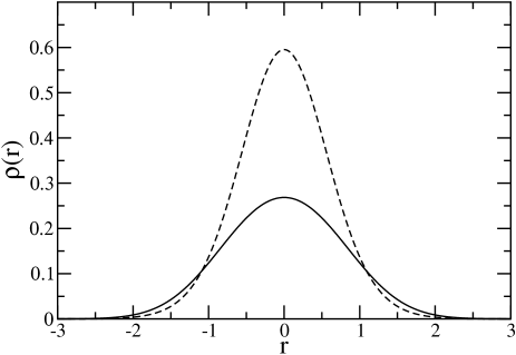
Figure 1: Density $\rho(r)=2|\psi_{1s}(r)|^{2}$ plotted along the $x$-axis, obtained from RHF calculations on a two-particle system in an isotropic trap with $a=0.2a_{x}$ (solid lines), and $a=-0.2a_{x}$ (dashed lines). Distance $r$ is in harmonic oscillator units.

5.2 Unrestricted Hartree-Fock Calculations

In this section we describe the results of our UHF calculations. If one performs a UHF calculation on a closed-shell system, one must get the same results as obtained by an RHF calculation. Similarly, the total energy and orbitals of a system with $m$ up-spin and $n$ down-spin particles should be the same as that of a system with $n$ up-spin and $m$ down-spin particles. These properties of the UHF calculations can be used to check the correctness of the underlying algorithm. We verified these properties explicitly by: (a) performing UHF calculations on closed-shell systems with various scattering lengths and geometries, and found that the results always agreed with the corresponding RHF calculations, and (b) by performing UHF calculations on various open-shell systems with interchanged spin configurations and found the results to be identical. Therefore, we are confident of the essential correctness of our UHF program, and in what follows, we describe its applications in calculating the addition energy of fermionic atoms confined in a spherical trap. The aim behind this calculation is to explore whether such a system follows: (a) shell-structure, and (b) Hund’s rule, in analogy with harmonically trapped electrons confined in a quantum dot. We also note that a study of Hund’s rule for fermionic atoms confined in an optical lattice was carried out recently by Kärkkäinen et al.[10].

The addition energy, i.e, the energy required to add an extra atom, to an $N$-atom trap is defined as $\Delta\mu(N)=\mu(N+1)-\mu(N)$, where $\mu(N)$/$\mu(N+1)$ represents the chemical potential of an $N/(N+1)$ particle system. The chemical potentials, in turn, are defined as $\mu(N)=E(N)-E(N-1)$, where $E(N)$/$E(N+1)$ represents the total energy of an $N/(N+1)$ particle system. In our calculations, the total energies were calculated using the UHF approach for various values of the scattering length and our results for the addition energy for an $a=0.01a_{x}$ spherical trap are presented in Fig. 2, for the values from $N=1$ to $N=21$ .

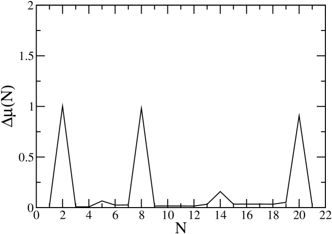
Figure 2: Calculated UHF values of addition energies ($\Delta\mu(N)=\mu(N+1)-\mu(N)$) of a spherical trap (in the units of $\hbar\omega_{x}$) with scattering length $a=0.01a_{x}$, plotted as a function of the particle number $N$, ranging from $N=1$ to $N=21$.

For the range of $N$ values studied here, in a noninteracting model the charging energy acquires nonzero values $\Delta\mu(N)=\hbar\omega_{x}$, only for $N=2,$ $8$, and $20$, corresponding to filled-shell configurations. In an interacting model, however, $\Delta\mu(N)$ should additionally exhibit smaller peaks at $N=5$, $N=14$, corresponding to the half-filled shells. If the inter-particle repulsion is strong enough to split $3s$ and $3d$ shells significantly, we will additionally obtain a peak at $N=18$ corresponding to the filled $3d$ shell, while the peaks corresponding to the half-filled shells will occur at $N=13$, and $N=19$, instead of $N=14$. Moreover, it is of considerable interest to examine whether the Hund’s rule is also satisfied for open-shell configurations of such spherically trapped fermionic atoms, as is the case, e.g., for electrons in quantum dots[11]. From Fig. 2 it is obvious that major peaks are located at $N=2,$ $8$, and $20$, while the minor ones are at $N=5$, and $14$, with no peaks at $N=13$, $18$, or $19$. The heights of the major peaks are in the descending order with increasing $N$, ranging from $1.003\hbar\omega_{x}$ ($N=2)$ to $0.908\hbar\omega_{x}$ ($N=20$). Additionally, for all the open-shell cases, the lowest-energy configurations were consistent with the Hund’s rule in that, a given shell is first filled with fermions of one (say ’up’) spin-orientation, and upon completion, followed by the fermions of other (’down’) spin orientation. We note that these results are qualitatively similar to the results obtained for spherical quantum dots[11]. Thus, we conclude that for the small number of particles considered by us, the shell structure and the Hund’s rule are also followed by atoms confined in harmonic traps where the mutual repulsion is through short-range the contact interaction.

We have performed a number of UHF calculations on traps of different geometries, and scattering lengths, whose results will be published elsewhere. However, we would like to briefly state that as the scattering length is increased, in several cases the ferromagnetic configurations violating the Hund’s rule become energetically more stable. This implies that for large scattering lengths the UHF mean-field approach may not be representative of the true state, and inclusion of correlation effects may be necessary.

6 Conclusions and Future Directions

In this paper we reported a Fortran 90 implementation of a harmonic oscillator basis set based approach towards obtaining the numerical solutions of both the restricted, as well as the unrestricted Hartree-Fock equations for spin-$\frac{1}{2}$ fermions confined by a harmonic potential, and interacting via pair-wise delta-function potential. The spin-$\frac{1}{2}$ fermions under consideration could represent a two-component fermi gas composed of atoms confined in harmonic traps. We performed a number of calculations assuming both attractive, and repulsive, inter-particle interactions. As expected, the Hartree-Fock method becomes unstable with the increasing scattering length for attractive interactions, while no such problem is encountered for the repulsive interactions. Additionally, we performed a UHF study of atoms confined in a spherical harmonic trap and verified the existence of a shell structure, and that the Hund’s rule is followed. These results are in good qualitative agreement with similar studies performed on harmonically confined electrons in quantum dots, interacting via Coulomb interaction.

In future, we intend to extend and improve the fermionic aspects of the present computer program in several possible ways. As far as problems related to fermionic gases in a trap are concerned, we would like to implement the Hartree-Fock-Bogoliubov approach to allow us to study such systems in the thermodynamic limit, and at finite temperatures. With the aim of studying the electronic structure of quantum dots, we plan to introduce the option of using the Coulomb-repulsion for interparticle interactions, a step which will require significant code writing for the two-electron matrix elements. Additionally, we also aim to introduce the option of studying the dynamics of electrons in the presence of an external magnetic field, which will also allow us to study fermionic gases in rotating traps. Finally, we plan to implement the option of including spin-orbit coupling in our approach, which, at present, is a very active area of research. We will report results along these lines in the future, as and when they become available.

References

- [1] See, e.g., K. M. O’Hara, S. L. Hemmer, M. E. Gehm, S. R. Granade, and, J. E. Thomas, Science 298 (2002) 2179; C. A. Regal, C. Ticknor, J. L. Bohn, and D. S. Jin, Nature 424 (2003) 47; M. Greiner, C. A. Regal, and D. S. Jin, 426 (2003) 537; S. Jochim, M. Bartenstein, A. Altmeyer, G. Hendl, S. Riedl, C. Chin, J. Hecker Denschlag, and R. Grimm, Science 302 (2003) 2101; M. W. Zwierlin, C. A. Stan, C. H. Schunk, S. M. F. Raupach, S. Gupta, Z. Hadzibabic, and W. Ketterle, Phys. Rev. Lett. 91 (2003) 250401;
- [2] M. W. Zwierlin, A. Schirotzek, C. H. Schunk, and W. Ketterle, Science 311 (2006) 492; G. B. Patridge, W. Li, R. I. Kamar, Y. Liao, R. G. Hulet, Science 311 (2006) 503; M. W. Zwierlin, C. H. Schunk, A. Schirotzek, and W. Ketterle, Nature 442 (2006) 54.
- [3] For a review, see, D. S. Petrov, C. Salomon, G. V. Shlyapnikov, J. Phys. B 38 (2005) S645; V. Gurarie and L. Radzihovsky, Ann. Phys. 322 (2002) 2, and references therein.
- [4] Y. Yu, M. Ögren, S. Åberg, S. M. Reimann, and M. Brack, Phys. Rev. A 72 (2005) 051602(R).
- [5] See, e.g., P. Pieri and G. C. Strinati, Phys. Rev. Lett. 96 (2006) 150404; K. B. Gubbels, M. W. J. Romans, and H. T. C. Stoof, Phys. Rev. Lett. 97 (2006) 210402.t
- [6] R. P. Tiwari and A. Shukla, Comp. Phys. Commun. 174 (2006) 966.
- [7] A. Szabo and N. Ostlund, Modern Quantum Chemistry, Introduction to Advanced Electronic Structure Theory, Dover Publications, Inc. (1989).
- [8] E. Anderson, Z. Bai, C. Bischof, S. Blackford, J. Demmel, J. Dongarra, J. Du Croz, A. Greenbaum, S. Hammarling, A. McKenney, and D. Sorensen, LAPACK Users’ Guide, 3rd Edn., (2002), SIAM, Philadelphia (USA).
- [9] E. R. I. Abraham, W. I. McAlexander, J. M. Gerton, R. G. Hulet, R. Côté, and A. Dalgarno, Phys. Rev. A 55 (1997) R3299.
- [10] K. Käkkäinen, M. Borgh, M. Manninen, and S. M. Reimann, New J. Phys. 9 (2007) 33.
- [11] See, e.g., Y. Asari, K. Takeda, and H. Tamura, Jpn. J. Appl. Phys. 43 (2004) 4424; C. F. Destefani, J. D. M. Vianna, and G. E. Marques, arxiv:physics/0404007.