Preconditioned HSS Method for Finite Element Approximations of Convection-Diffusion Equations

Abstract

A two-step preconditioned iterative method based on the Hermitian/Skew-Hermitian splitting is applied to the solution of nonsymmetric linear systems arising from the Finite Element approximation of convection-diffusion equations. The theoretical spectral analysis focuses on the case of matrix sequences related to FE approximations on uniform structured meshes, by referring to spectral tools derived from Toeplitz theory. In such a setting, if the problem is coercive, and the diffusive and convective coefficients are regular enough, then the proposed preconditioned matrix sequence shows a strong clustering at unity, i.e., a superlinear preconditioning sequence is obtained. Under the same assumptions, the optimality of the PHSS method is proved and some numerical experiments confirm the theoretical results. Tests on unstructured meshes are also presented, showing the some convergence behavior.

1 Introduction

The paper deals with the numerical solution of linear systems arising from the Finite Element approximation of the elliptic convection-diffusion problem

$$\left\{\begin{array}[]{l}\mathrm{div}\left(-a(\mathbf{x})\nabla u+\vec{\mathbf{\beta}}(\mathbf{x})u\right)=f,\quad\mathbf{x}\in\Omega,\\ u_{|\partial\Omega}=0.\end{array}\right.$$ (1)

We apply the two-step iterative method based on the Hermitian/Skew-Hermitian splitting (HSS) of the coefficient matrix proposed in [3] for the solution of nonsymmetric linear systems whose real part is coercive. The aim is to study the preconditioning effectiveness when the Preconditioned HSS (PHSS) method is applied, as proposed in [5]. According to the PHSS convergence properties, the preconditioning strategy for the matrix sequence $\{A_{n}(a,\vec{\mathbf{\beta}})\}$ can be tuned only with respect to the stiffness matrices. This allows to adopt the same preconditioning proposal just analyzed in the case of Finite Difference (FD) and Finite Element (FE) approximations of the diffusion problem in [17, 19, 20, 22, 23, 21, 4], and, more recently, in the case of FD approximations of (1).
More precisely, we consider the preconditioning matrix sequence $\{P_{n}(a)\}$ defined as $P_{n}(a)=D_{n}^{{1}/{2}}(a)A_{n}(1,0)D_{n}^{{1}/{2}}(a)$, where $D_{n}(a)=\mathrm{diag}(A_{n}(a,0))\mathrm{diag}\!^{-1}(A_{n}(1,0))$, i.e., the suitable scaled main diagonal of $A_{n}(a,0)$. In such a way, the solution of the linear system with coefficient matrix $A_{n}(a,\vec{\mathbf{\beta}})$ is reduced to computations involving diagonals and the matrix $A_{n}(1,0)$. In the case of uniform structured meshes the latter task can be efficiently performed by means of fast Poisson solvers, among which we can list those based on the cyclic reduction idea (see e.g. [8, 10, 25]) and several specialized multigrid methods (see e.g. [13, 18]).
Our theoretical analysis focuses on the case of matrix sequences $\{A_{n}(a,\vec{\mathbf{\beta}})\}$ related to FE approximations on uniform structured meshes, since the powerful spectral tools derived from Toeplitz theory [6, 7, 15, 16] greatly facilitate the required spectral analysis. In such a setting, under proper assumptions on $a(\mathbf{x})$ and $\vec{\mathbf{\beta}}(\mathbf{x})$, we prove the optimality of the PHSS method. In our terminology (see [2]) this means that the PHSS iterations number for reaching the solution within a fixed accuracy can be bounded from above by a constant independent of the dimension $n=n(h)$.
Nevertheless, the numerical experiments have been performed also in the case of unstructured meshes, with negligible differences in the PHSS method performances. In such cases, by coupling the PHSS method with standard Preconditioned Conjugate Gradient (PCG) and Preconditioned Generalized Minimal Residual (PGMRES) method, our proposal makes only use of matrix vector products (for sparse or even diagonal matrices) and of a solver for the related diffusion equation with constant coefficient.
The underlying idea is that whenever $P_{n}(a)$ results to be an approximate factorization of $A_{n}(a,\vec{\mathbf{\beta}})$, the computational bottleneck lies in the solution of linear systems with coefficient matrix $A_{n}(1,0)$. Thus, the main effort in devising efficient algorithms must be devoted to this simpler problem. Moreover, to some extent, the approximation schemes in the discretization should take into account this key step to give rise to a linear algebra problem less difficult to cope with.

The outline of the paper is as follows. In section 2 we report a brief description of the FE approximation of the convection-diffusion equation, while in section 3 we summarize the definition and the convergence properties of the Hermitian/Skew-Hermitian (HSS) method and of its preconditioned formulation (PHSS method). Section 4 analyzes the spectral properties of the matrix sequences arising from FE approximations of the considered convection-diffusion problem and reports the preconditioner definition. Section 5 is devoted to the theoretical analysis of the preconditioned matrix sequence spectral properties in the case of structured uniform meshes. In section 6 several numerical experiments illustrate the claimed convergence properties and their extension in the case of other structured and unstructured meshes. Lastly, section 7 deals with complexity issues and perspectives.

2 Finite Element approximation

Problem (1) can be stated in variational form as follows:

$$\left\{\begin{array}[]{l}\textrm{find $u\in H_{0}^{1}(\Omega)$ such that}\\ \int_{\Omega}\left(a\nabla u\cdot\nabla\varphi-\vec{\mathbf{\beta}}\cdot\nabla\varphi\ u\right)=\int_{\Omega}f\varphi\quad\textrm{for all }\varphi\in H_{0}^{1}(\Omega)\end{array}\right.$$ (2)

where $H_{0}^{1}(\Omega)$ is the space of square integrable functions, with ${L}^{2}$ weak derivatives vanishing on $\partial\Omega$. We assume that $\Omega$ is a polygonal domain and we make the following hypotheses on the coefficients

$$\left\{\begin{array}[]{l}a\in{\bf C}^{2}(\overline{\Omega}),\quad\textrm{ with }a(\mathbf{x})\geq a_{0}>0,\\ \vec{\mathbf{\beta}}\in{\bf C}^{1}(\overline{\Omega}),\quad\textrm{ with }\mathrm{div}\vec{\mathbf{\beta}}\geq 0\textrm{ pointwise in }\Omega,\\ f\in{L}^{2}(\Omega).\end{array}\right.$$ (3)

The previous assumptions guarantee existence and uniqueness for problem (2).
For the sake of simplicity, we restrict ourselves to linear finite element approximation of problem (2). To this end, let $\mathcal{T}_{h}=\{K\}$ be a usual finite element partition of $\overline{\Omega}$ into triangles, with $h_{K}=\mathrm{diam}(K)$ and $h=\max_{K}{h_{K}}$. Let $V_{h}\subset H^{1}_{0}(\Omega)$ be the space of linear finite elements, i.e.

$$V_{h}=\{\varphi_{h}:\overline{\Omega}\rightarrow\mathbb{R}\ \textrm{ s.t. }\varphi_{h}\textrm{ is continuous, }{\varphi_{h}}_{|_{K}}\textrm{ is linear, and }{\varphi_{h}}_{|\partial\Omega}=0\}.$$

The finite element approximation of problem (2) reads:

$$\left\{\begin{array}[]{l}\textrm{find $u_{h}\in V_{h}$ such that}\\ \int_{\Omega}\left(a\nabla u_{h}\cdot\nabla\varphi_{h}-\vec{\mathbf{\beta}}\cdot\nabla\varphi_{h}\ u_{h}\right)=\int_{\Omega}f\varphi_{h}\quad\textrm{for all }\varphi_{h}\in V_{h}.\end{array}\right.$$ (4)

For each internal node $i$ of the mesh $\mathcal{T}_{h}$, let $\varphi_{i}\in V_{h}$ be such that $\varphi_{i}(\textrm{node }i)=1$, and $\varphi_{i}(\textrm{node }j)=0$ if $i\neq j$. Then, the collection of all $\varphi_{i}$’s is a base for $V_{h}$. We will denote by $n(h)$ the number of the internal nodes of $\mathcal{T}_{h}$, which corresponds to the dimension of $V_{h}$. Then, we write $u_{h}$ as

$$u_{h}=\sum_{i=1}^{n(h)}u_{i}\varphi_{i}$$

and the variational equation (4) becomes an algebraic linear system:

$$\sum_{j=1}^{n(h)}\left(\int_{\Omega}a\nabla\varphi_{j}\cdot\nabla\varphi_{i}-\nabla\varphi_{i}\cdot\vec{\mathbf{\beta}}\ \varphi_{j}\right)u_{j}=\int_{\Omega}f\varphi_{i},\quad i=1,\ldots,n(h).$$ (5)

The aim of this paper is to study the effectiveness of the proposed Preconditioned HSS method applied to the quoted nonsymmetric linear systems (5), both from the theoretical and numerical point of view.

3 Preconditioned HSS method

In this section we briefly summarize the definition and the relevant properties of the Hermitian/Skew-Hermitian (HSS) method formulated in [3] and of its extension in the case of preconditioning as proposed in [5].
The HSS method can be applied whenever we are looking for the solution of a linear system $A_{n}\mathbf{x}=\mathbf{b}$ where $A_{n}\in\mathbb{C}^{n\times n}$ is a non singular matrix with a positive definite real part and $\mathbf{x},\mathbf{b}$ belong to $\mathbb{C}^{n}$. Several applications in scientific computing lead to such kind of linear problems and, typically, the matrix $A_{n}$ is also large and sparse, as in the case of FD or FE approximations of (1).
More in detail, the HSS method refers to the unique Hermitian/Skew-Hermitian splitting of the matrix $A_{n}$ as

$$A_{n}=\mathrm{Re}(A_{n})+\mathrm{i}\,\mathrm{Im}(A_{n}),\quad\mathrm{i}^{2}=-1$$ (6)

where

$$\mathrm{Re}(A_{n})=\frac{A_{n}+A_{n}^{H}}{2}\quad\mathrm{and}\quad\mathrm{Im}(A_{n})=\frac{A_{n}-A_{n}^{H}}{2\mathrm{i}}$$

are Hermitian matrices by definition.
In the same spirit of the ADI method [11], the quoted splitting allows to define the Hermitian/Skew-Hermitian (HSS) method [3], as follows

$$\left\{\begin{array}[]{lcl}\left(\alpha I+\mathrm{Re}(A_{n})\right)\mathbf{x}^{k+{1\over 2}}&=&\left(\alpha I-\mathrm{i}\,\mathrm{Im}(A_{n})\right)\mathbf{\mathbf{x}}^{k}+\mathbf{b}\\ \left(\alpha I+\mathrm{i}\,\mathrm{Im}(A_{n})\right)\mathbf{x}^{k+1}&=&\left(\alpha I-\mathrm{Re}(A_{n})\right)\mathbf{x}^{k+{1\over 2}}+\mathbf{b}\end{array}\right.$$ (7)

with $\alpha$ positive parameter and $\mathbf{x}^{0}$ given initial guess.
Beside the quoted formulation as a two-step iteration method, the HSS method can be reinterpreted as a stationary iterative method whose iteration matrix is given by

$$\widetilde{M}(\alpha)=\left(\alpha I+\mathrm{i}\,\mathrm{Im}(A_{n})\right)^{-1}\left(\alpha I-\mathrm{Re}(A_{n})\right)\left(\alpha I+\mathrm{Re}(A_{n})\right)^{-1}\left(\alpha I-\mathrm{i}\,\mathrm{Im}(A_{n})\right)$$ (8)

and whose convergence properties are only related to the spectral radius of the Hermitian matrix $\left(\alpha I-\mathrm{Re}(A_{n})\right)\left(\alpha I+\mathrm{Re}(A_{n})\right)^{-1}$, which is unconditionally bounded by $1$ provided the positivity of $\alpha$ and of $\mathrm{Re}(A_{n})$ [3].
Indeed, the rate of convergence can be unsatisfactory for large values of $n$ in the case of PDEs applications, as for instance (1), so that the preconditioned formulation of the method proposed in [5] is more profitable.
Let $P_{n}$ be a Hermitian positive definite matrix. The Preconditioned HSS (PHSS) method can be defined as

$$\left\{\begin{array}[]{lcl}\left(\alpha I+P_{n}^{-1}\mathrm{Re}(A_{n})\right)\mathbf{x}^{k+{1\over 2}}&=&\left(\alpha I-P_{n}^{-1}\mathrm{i}\,\mathrm{Im}(A_{n})\right)\mathbf{x}^{k}+P_{n}^{-1}\mathbf{b}\\ \left(\alpha I+P_{n}^{-1}\mathrm{i}\,\mathrm{Im}(A_{n})\right)\mathbf{x}^{k+1}&=&\left(\alpha I-P_{n}^{-1}\mathrm{Re}(A_{n})\right)\mathbf{x}^{k+{1\over 2}}+P_{n}^{-1}\mathbf{b}\end{array}\right.$$ (9)

Notice that the proposed method differs from the HSS method applied to the matrix $P_{n}^{-1}A_{n}$ since $P_{n}^{-1}\mathrm{Re}(A_{n})$ and $P_{n}^{-1}\mathrm{Im}(A_{n})$ are not the Hermitian/Skew-Hermitian splitting of $P_{n}^{-1}A_{n}$.
Let $\lambda(X)$ denote the set of the eigenvalues of a square matrix $X$; the convergence properties of the PHSS method exactly mimic those of the previous HSS method, as claimed in the theorem below.

Theorem 1.

[5] Let $A_{n}\in\mathbb{C}^{n\times n}$ be a matrix with positive definite real part, $\alpha$ be a positive parameter and let $P_{n}\in\mathbb{C}^{n\times n}$ be a Hermitian positive definite matrix. Then the iteration matrix of the PHSS method is given by

$$M(\alpha) = \left(\alpha I+\mathrm{i}\,P_{n}^{-1}\mathrm{Im}(A_{n})\right)^{-1}\left(\alpha I-P_{n}^{-1}\mathrm{Re}(A_{n})\right)\left(\alpha I+P_{n}^{-1}\mathrm{Re}(A_{n})\right)^{-1}$$

$$\left(\alpha I-\mathrm{i}\,P_{n}^{-1}\mathrm{Im}(A_{n})\right),$$

its spectral radius $\varrho(M(\alpha))$ is bounded by

$$\sigma(\alpha)=\max_{\lambda_{i}\in\lambda(P_{n}^{-1}{\rm Re}(A_{n}))}\left|{\alpha-\lambda_{i}\over\alpha+\lambda_{i}}\right|<1\quad\textrm{for any}\quad\alpha>0,$$

i.e., the PHSS iteration is unconditionally convergent to the unique solution of the system $A_{n}\mathbf{x}=\mathbf{b}$. Moreover, denoting by $\kappa={\lambda_{\max}(P_{n}^{-1}\mathrm{Re}(A_{n}))}/{\lambda_{\min}(P_{n}^{-1}\mathrm{Re}(A_{n}))}$ the spectral condition number (namely the Euclidean (spectral) condition number of the symmetrized matrix), the optimal $\alpha$ value that minimizes the quantity $\sigma(\alpha)$ equals

$$\alpha^{*}=\sqrt{\lambda_{\min}(P_{n}^{-1}\mathrm{Re}(A_{n}))\lambda_{\max}(P_{n}^{-1}\mathrm{Re}(A_{n}))}\quad\mathrm{and}\quad\sigma(\alpha^{*})={\sqrt{\kappa}-1\over\sqrt{\kappa}+1}.$$

Thus, the unconditional convergence property holds also in the preconditioned formulation of the method and the convergence properties are related to the spectral radius of

$$\left(\alpha I-P_{n}^{-1/2}\mathrm{Re}(A_{n})P_{n}^{-1/2}\right)\left(\alpha I+P_{n}^{-1/2}\mathrm{Re}(A_{n})P_{n}^{-1/2}\right)^{-1},$$

where the optimal parameter $\alpha$ is the square root of the product of the extreme eigenvalues of $P_{n}^{-1}\mathrm{Re}(A_{n})$.
It is worth stressing that the PHSS method in (9) can also be interpreted as the original iteration (7) where the identity matrix is replaced by the preconditioner $P_{n}$, i.e.,

$$\left\{\begin{array}[]{lcl}\left(\alpha P_{n}+\mathrm{Re}(A_{n})\right)\mathbf{x}^{k+{1\over 2}}&=&\left(\alpha P_{n}-\mathrm{i}\ \mathrm{Im}(A_{n})\right)\mathbf{x}^{k}+\mathbf{b}\\ \left(\alpha P_{n}+\mathrm{i}\ \mathrm{Im}(A_{n})\right)\mathbf{x}^{k+1}&=&\left(\alpha P_{n}-\mathrm{Re}(A_{n})\right)\mathbf{x}^{k+{1\over 2}}+\mathbf{b}\end{array}\right.$$ (10)

Clearly, the last formulation is the most interesting from a practical point of view, since it does not involve any inverse matrix and it easily allows to define an inexact formulation of the quoted method: in principle, at each iteration, the PHSS method requires the exact solutions with respect to the large matrices $\alpha P_{n}+\mathrm{Re}(A_{n})$ and $\alpha P_{n}+\mathrm{i}\,\mathrm{Im}(A_{n})$. This requirement is impossible to achieve in practice and an inexact outer iteration is computed by applying a Preconditioned Conjugate Gradient method (PCG) and a Preconditioned Generalized Minimal Residual method (PGMRES), with preconditioner $P_{n}$, to the coefficient matrices $\alpha P_{n}+\mathrm{Re}(A_{n})$ and $\alpha P_{n}+\textrm{i}\ \mathrm{Im}(A_{n})$, respectively. Hereafter, we denote by IPHSS method the described inexact PHSS iterations.
The accuracy for the stopping criterion of these additional inner iterative procedures must be chosen by taking into account the accuracy obtained by the current step of the outer iteration (see [3, 5] and section 6 for some remarks about this topic). The most remarkable fact is that the PHSS and IPHSS methods show the same convergence properties, though the computational cost of the latter is substantially reduced with respect to the former.
In the IPHSS perspective the spectral properties induced by the preconditioner $P_{n}$ are relevant not only with respect to the IPHSS rate of convergence, i.e., the outer iteration, but also with respect to the PCG and PGMRES ones. So, the spectral analysis of the matrix sequence $\{P_{n}^{-1}\mathrm{Im}(A_{n})\}$ becomes relevant exactly as the spectral analysis of the matrix sequence $\{P_{n}^{-1}\mathrm{Re}(A_{n})\}$.
Lastly, it is worth stressing that a deeper insight of the HSS/PHSS convergence properties with respect to the skew-Hermitian part pertains to the framework of multi-iterative methods [14], among which multigrid methods represent a classical example. Typically, a multi-iterative method is composed by two, or more, different iterative techniques, where each one is cheap and potentially slow convergent. Nevertheless, these iterations have a complementary spectral behavior, so that their composition becomes fast convergent. In fact, the PHSS matrix iteration can be reinterpreted as the composition of two distinct iteration matrices and the strong complementarity of these two components makes the contraction factor of the whole procedure much smaller than the contraction factors of the two distinct components. In particular, the skew-Hermitian contributions in the iteration matrix can have a role in accelerating the convergence. The larger is $\vec{\mathbf{\beta}}(\mathbf{x})$, i.e., the problem is convection dominated, the more the FE matrix $A_{n}$ departs from normality. Thus, a stronger “mixing up effect” is observed and the real convergence behavior of the method is much faster compared with the forecasts of Theorem 1. See [5] for further details.

4 Preconditioning strategy

According to the notations and definitions in Section 2, the algebraic equations in (5) can be rewritten in matrix form as the linear system

$$A_{n}(a,\vec{\mathbf{\beta}})\mathbf{x}=\mathbf{b},$$

with

$$A_{n}(a,\vec{\mathbf{\beta}})=\Theta_{n}(a)+\Psi_{n}(\vec{\mathbf{\beta}})\in\mathbb{R}^{n\times n},\ n=n(h),$$ (11)

where $\Theta_{n}(a)$ and $\Psi_{n}(\vec{\mathbf{\beta}})$ represent the approximation of the diffusive term and approximation of the convective term, respectively. More precisely, we have

$$(\Theta_{n}(a))_{i,j} = \int_{\Omega}a\nabla\varphi_{i}\nabla\varphi_{j}$$ (12)

$$(\Psi_{n}(\vec{\mathbf{\beta}}))_{i,j} = -\int_{\Omega}(\nabla\varphi_{i}\cdot\vec{\mathbf{\beta}})\ \varphi_{j},$$ (13)

where suitable quadrature formula are considered in the case of non constant coefficient functions $a$ and $\vec{\mathbf{\beta}}$.
Thus, according to (6), the Hermitian/skew-Hermitian decomposition of $A_{n}(a,\vec{\mathbf{\beta}})$ is given by

$$\mathrm{Re}(A_{n}(a,\vec{\mathbf{\beta}})) = \Theta_{n}(a)+\mathrm{Re}(\Psi_{n}(\vec{\mathbf{\beta}})),$$ (14)

$$\mathrm{i}\,\mathrm{Im}(A_{n}(a,\vec{\mathbf{\beta}})) = \mathrm{i}\,\mathrm{Im}(\Psi_{n}(\vec{\mathbf{\beta}})),$$ (15)

where

$$\mathrm{Re}(\Psi_{n}(\vec{\mathbf{\beta}})) = \frac{1}{2}(\Psi_{n}(\vec{\mathbf{\beta}})+\Psi_{n}^{T}(\vec{\mathbf{\beta}}))=E_{n}(\vec{\mathbf{\beta}}),$$

$$\mathrm{i}\,\mathrm{Im}(\Psi_{n}(\vec{\mathbf{\beta}})) = \Psi_{n}(\vec{\mathbf{\beta}})-E_{n}(\vec{\mathbf{\beta}}),$$

since by definition, the diffusion therm $\Theta_{n}(a)$ is a Hermitian matrix and does not contribute to the skew-Hermitian part of $A_{n}(a,\vec{\mathbf{\beta}})$. Notice also that $E_{n}(\vec{\mathbf{\beta}})=0$ if $\mathrm{div}(\vec{\mathbf{\beta}})=0$.
Clearly, the quoted HSS decomposition can be performed on any single elementary matrix related to $\mathcal{T}_{h}$ by considering the standard assembling procedure.
By construction, the matrix $\mathrm{Re}(A_{n}(a,\vec{\mathbf{\beta}}))$ is symmetric and positive definite whenever $\lambda_{\min}(\Theta_{n}(a))\geq\rho(E_{n}(\vec{\mathbf{\beta}}))$. Indeed, without the condition $\mathrm{div}(\vec{\mathbf{\beta}})\geq 0$, the matrix $E_{n}(\vec{\mathbf{\beta}})$ does not have a definite sign.
Moreover, the Lemma below allows to obtain further information regarding such a structural assumption.

Lemma 2.

Let $\{E_{n}(\vec{\mathbf{\beta}})\}$ be the matrix sequence defined as

$$E_{n}(\vec{\mathbf{\beta}})=\frac{1}{2}(\Psi_{n}(\vec{\mathbf{\beta}})+\Psi_{n}^{T}(\vec{\mathbf{\beta}})).$$

Under the assumptions in (3), then it holds

$$\|E_{n}(\vec{\mathbf{\beta}})\|_{2}\leq\|E_{n}(\vec{\mathbf{\beta}})\|_{\infty}\leq Ch^{2},$$

with $C$ absolute positive constant only depending on $\vec{\mathbf{\beta}}(\mathbf{x})$ and $\Omega$.

Proof.

By applying the Green formula, it holds that for any $i,j=1,\ldots,n(h)$

$$(E_{n}(\vec{\mathbf{\beta}}))_{i,j} = -\frac{1}{2}\int_{\Omega}\left((\nabla\varphi_{i}\cdot\vec{\mathbf{\beta}})\varphi_{j}+(\nabla\varphi_{j}\cdot\vec{\mathbf{\beta}})\varphi_{i}\right)=-\frac{1}{2}\int_{\Omega}\vec{\mathbf{\beta}}\cdot\nabla(\varphi_{i}\varphi_{j})$$

$$= \frac{1}{2}\int_{\Omega}\mathrm{div}(\vec{\mathbf{\beta}})\cdot\varphi_{i}\varphi_{j}$$

$$= \frac{1}{2}\sum_{K\subseteq S(\varphi_{i})\cap S(\varphi_{j})}\int_{K}\mathrm{div}(\vec{\mathbf{\beta}})\varphi_{i}\varphi_{j},$$

with respect to the related mesh $\mathcal{T}_{h}=\{K\}$ and where $S(\varphi_{k})$ denotes the support of basis element $\varphi_{k}$ on $\mathcal{T}_{h}$. Thus, we have

$$|E_{n}(\vec{\mathbf{\beta}})|_{i,j}\leq\frac{1}{2}\sup_{\Omega}\left|\mathrm{div}(\vec{\mathbf{\beta}})\right|\sum_{K\subseteq S(\varphi_{i})\cap S(\varphi_{j})}\int_{K}|\varphi_{i}\varphi_{j}|\leq\frac{1}{4}\sup_{\Omega}\left|\mathrm{div}(\vec{\mathbf{\beta}})\right|qh^{2}$$

since $|\varphi_{k}|\leq 1$ for any $k$ and

$$\sum_{K\subseteq S(\varphi_{i})\cap S(\varphi_{j})}\int_{K}|\varphi_{i}\varphi_{j}|\leq\frac{h^{2}}{2}\#\{K\in\mathcal{T}_{h}|K\subseteq S(\varphi_{i})\cap S(\varphi_{j})\}\leq\frac{qh^{2}}{2},$$

where $h$ is the finesse parameter of the mesh $\mathcal{T}_{h}$ and $q$ equals the maximum number of involved mesh elements with respect to the mesh sequence $\{\mathcal{T}_{h}\}$.
Lastly, since $E_{n}(\vec{\mathbf{\beta}})$ is a Hermitian matrix, it holds

$$\|E_{n}(\vec{\mathbf{\beta}})\|_{2}\leq\|E_{n}(\vec{\mathbf{\beta}})\|_{\infty}\leq D\max_{i,j=1,\ldots,n(h)}|E_{n}(\vec{\mathbf{\beta}})|_{i,j}\leq\frac{1}{4}D\sup_{\Omega}|\mathrm{div}(\vec{\mathbf{\beta}})|qh^{2},$$

where $D$ denotes the maximum number of nonzero entries on the rows of $E_{n}(\vec{\mathbf{\beta}})$. ∎

Remark 3.

The claim of Lemma 2 holds whenever a quadrature formula with error $O(h^{2})$ is consider for approximating the integrals involved in (13).

Moreover, in the special case of a structured uniform mesh on $\Omega=(0,1)^{2}$ as considered in the next section, under the assumptions of Lemma 2 and $a(\mathbf{x})\geq a_{0}>0$, we have $\Theta_{n}(a)\geq ch^{2}I_{n}$ (with $c$ absolute positive constant), so that $\mathrm{Re}(A_{n}(a,\vec{\mathbf{\beta}}))\geq(c-C)h^{2}I_{n}$. Here, we are referring to the standard ordering relation between Hermitian matrices, i.e., the notation $X\geq Y$, with $X$ and $Y$ Hermitian matrices, means that $X-Y$ is nonnegative definite. Thus, under the assumption that $|\mathrm{div}(\vec{\mathbf{\beta}})|$ is smaller than a positive suitable constant, it holds that $\mathrm{Re}(A_{n}(a,\vec{\mathbf{\beta}}))$ is real, symmetric, and positive definite.
However, the main drawback is due to ill-conditioning, since the condition number is asymptotic to $h^{-2}$, so that preconditioning is highly recommended.
By referring to a preconditioning strategy previously analyzed in the case of FD approximations [17, 19, 20, 22, 23] or FE approximations [21] of the diffusion equation and recently applied to FD approximations [5] of (1), we consider the preconditioning matrix sequence $\{P_{n}(a)\}$ defined as

$$P_{n}(a)=D_{n}^{\frac{1}{2}}(a)A_{n}(1,0)D_{n}^{\frac{1}{2}}(a)$$ (16)

where $D_{n}(a)=\mathrm{diag}(A_{n}(a,0))\mathrm{diag}^{-1}(A_{n}(1,0))$, i.e., the suitable scaled main diagonal of $A_{n}(a,0)$ and clearly $A_{n}(a,0)$ equals $\Theta_{n}(a)$.
In such a way, the solution of the linear system $A_{n}(a,\vec{\mathbf{\beta}})\mathbf{u}=\mathbf{f}$ is reduced to computations involving diagonals and the matrix $A_{n}(1,0)$. In the case of uniform structured mesh this task can be efficiently performed by considering fast Poisson solvers, such as those based on the cyclic reduction idea (see e.e. [8, 10, 25]) and several specialized multigrid methods (see e.g. [13, 18]).
It is worth stressing that the preconditioner is tuned only with respect to the diffusion matrix $\Theta_{n}(a)$ owing to the PHSS convergence properties highlighted in section 3. Indeed, the PHSS shows a convergence behavior mainly depending on the spectral properties of the matrix $P_{n}^{-1}(a)\mathrm{Re}(A_{n}(a,\vec{\mathbf{\beta}}))$. Nevertheless, the skew-Hermitian contribution may play a role in speeding up considerably the convergence (see [5] for further details).
Hereafter, we denote by $\{A_{n}(a,\vec{\mathbf{\beta}})\}$, $n=n(h)$ the matrix sequence associated to a family of mesh $\{T_{h}\}$, with decreasing finesse parameter $h$. As customary, the whole preconditioning analysis will refer to a matrix sequence instead to a single matrix, since the goal is to quantify the difficult of the linear system resolution in relation to the accuracy of the chosen approximation scheme.

5 Spectral analysis and clustering properties in the case of structured uniform meshes

In the present section we analyze the spectral properties of the preconditioned matrix sequences

$$\{P_{n}^{-1}(a)\mathrm{Re}(A_{n}(a,\vec{\mathbf{\beta}}))\}\ \mathrm{and}\ \{P_{n}^{-1}(a)\mathrm{Im}(A_{n}(a,\vec{\mathbf{\beta}}))\}$$

in the special case of $\Omega=(0,1)^{2}$ with a structured uniform mesh as in Figure 1, by using the spectral tools derived from Toeplitz theory [6, 7, 15, 16]. The aim is to prove the optimality of the PHSS method, i.e., the PHSS iterations number for reaching the solution within a fixed accuracy can be bounded from above by a constant independent of the dimension $n=n(h)$. A more in depth analysis is also considered for foreseeing the IPHSS method convergence behavior.

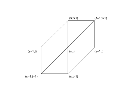
Fig. 1: Uniform structured mesh giving rise to a Toeplitz matrix in the constant coefficient case $a(\mathbf{x})=1$.

We make reference to the following definition.

Definition 4.

[26] Let $\{A_{n}\}$ be a sequence of matrices of increasing dimensions $n$ and let $g$ be a measurable function defined over a set $K$ of finite and positive Lebesgue measure. The sequence $\{A_{n}\}$ is distributed as the measurable function $g$ in the sense of the eigenvalues, i.e., $\{A_{n}\}\sim_{\lambda}g$ if, for every $F$ continuous, real valued and with bounded support, we have

$$\lim_{n\to\infty}\frac{1}{n}\sum_{j=1}^{n}F\left(\lambda_{j}\bigl{(}A_{n}\bigr{)}\right)={1\over m\{K\}}\int_{K}F(\theta(s))\,ds,$$

where $\lambda_{j}(A_{n})$, $j=1,\ldots,n$, denote the eigenvalues of $A_{n}$.
The sequence $\{A_{n}\}$ is clustered at $p$ if it is distributed as the constant function $g(x)\equiv p$, i.e., for any $\varepsilon>0$, $\#\left\{i\left.\right|\lambda_{i}(A_{n})\notin(p-\varepsilon,p+\varepsilon)\right\}=o(n)$. The sequence $\{A_{n}\}$ is properly (or strongly) clustered at $p$ if for any $\varepsilon>0$ the number of the eigenvalues of $A_{n}$ not belonging to $(p-\varepsilon,p+\varepsilon)$ can be bounded by a pure constant eventually depending on $\varepsilon$, but not on $n$.

First, we analyze the spectral properties of the matrix sequence $\{P_{n}^{-1}(a)\mathrm{Re}(A_{n}(a,\vec{\mathbf{\beta}}))\}$ that directly influences the convergence behavior of the PHSS method. We refer to a preliminary result in the case in which the convection term is not present.

Theorem 5.

[21] Let $\{A_{n}(a,\mathbf{0})\}$ and $\{P_{n}(a)\}$ be the Hermitian positive definite matrix sequences defined according to (11) and (16). If the coefficient $a(\mathbf{x})$ is strictly positive and belongs to ${\bf C}^{2}(\overline{\Omega})$, then the sequence $\{P_{n}^{-1}(a)A_{n}(a,\mathbf{0})\}$ is properly clustered at $1$. Moreover, for any $n$ all the eigenvalues of $P_{n}^{-1}(a)A_{n}(a,\mathbf{0})$ belong to an interval $[d,D]$ well separated from zero [Spectral equivalence property].  

The extension of this claim in the case of the matrix sequence $\{\mathrm{Re}(A_{n}(a,\vec{\mathbf{\beta}}))\}$ with $\mathrm{Re}(A_{n}(a,\vec{\mathbf{\beta}}))\neq\Theta_{n}(a)$ can be proved under the additional assumptions of Lemma 2.

Theorem 6.

Let $\{\mathrm{Re}(A_{n}(a,\vec{\mathbf{\beta}}))\}$ and $\{P_{n}(a)\}$ be the Hermitian positive definite matrix sequences defined according to (14) and (16). Under the assumptions in (3), then the sequence $\{P_{n}^{-1}(a)\mathrm{Re}(A_{n}(a,\vec{\mathbf{\beta}}))\}$ is properly clustered at $1$. Moreover, for any $n$ all the eigenvalues of $P_{n}^{-1}(a)\mathrm{Re}(A_{n}(a,\vec{\mathbf{\beta}}))$ belong to an interval $[d,D]$ well separated from zero [Spectral equivalence property].

Proof.

The proof technique refers to a previously analyzed FD case [22] and it is extended for dealing with the additional contribution given by $E_{n}(\vec{\mathbf{\beta}})$.
First, we consider the spectral equivalence property. Due to a similarity argument, we analyze the sequence $\{\Theta_{n}^{-1}(1)(\Theta_{n}^{*}(a)+E_{n}^{*}(\vec{\mathbf{\beta}}))\}$, where $X^{*}=D_{n}^{-\frac{1}{2}}(a)XD_{n}^{-\frac{1}{2}}(a)$ and $D_{n}(a)=\mathrm{diag}(\Theta_{n}(a))\mathrm{diag}^{-1}(\Theta_{n}(1))$. According to the assumptions and Theorem 7 in [21], we have the following asymptotic expansion

$$\Theta_{n}^{*}(a)=\Theta_{n}(1)+h^{2}F_{m}(a)+o(h^{2})G_{n}(a)$$ (17)

so that

$$\Theta_{n}^{-1}(1)\Theta_{n}^{*}(a)=I_{n}+\Theta_{n}^{-1}(1)(h^{2}F_{n}(a)+o(h^{2})G_{n}(a)).$$

Taking into account the order of the zeros of the generating function of the Toeplitz matrix $\Theta_{n}(1)$, we infer that there exists a constant $c_{1}$ so that $\|\Theta_{n}^{-1}(1)\|_{2}\leq c_{1}h^{-2}$ [6, 15]. Moreover, it also holds that

$$\|E_{n}^{*}(\vec{\mathbf{\beta}})\|_{2}\leq\frac{Ch^{2}}{\min_{\Omega}a}.$$ (18)

Therefore, by standard linear algebra, we have

$$\lambda_{\max}(\Theta_{n}^{-1}(1)(\Theta_{n}^{*}(a)+E_{n}^{*}(\vec{\mathbf{\beta}})) \leq \|\Theta_{n}^{-1}(1)(\Theta_{n}^{*}(a)+E_{n}^{*}(\vec{\mathbf{\beta}}))\|_{2}$$

$$\leq \|I_{n}\|_{2}+h^{2}\|\Theta_{n}^{-1}(1)\|_{2}\|F_{n}(a)+o(1)G_{n}(a)\|_{2}$$

$$\quad+\|\Theta_{n}^{-1}(1)\|_{2}\|E_{n}^{*}(\vec{\mathbf{\beta}})\|_{2}$$

$$\leq 1+c_{1}\left(\|F_{n}(a)\|_{2}+o(1)\|G_{n}(a)\|_{2}+\frac{C}{\min_{\Omega}a}\right),$$

where $\|F_{n}(a)\|_{2}$ and $\|G_{n}(a)\|_{2}$ are uniformly bounded since $F_{n}(a)$ and $G_{n}(a)$ are bounded symmetric sparse matrices by virtue of Theorem 7 in [21].
Conversely, a bound from below for $\lambda_{\min}(\Theta_{n}^{-1}(1)(\Theta_{n}^{*}(a)+E_{n}^{*}(\vec{\mathbf{\beta}}))$ requires a bit different technique with respect to Theorem 5, owing to the presence of the convective term. Again by a similarity argument and by referring to the Courant-Fisher Theorem, we have

$$\lambda_{\min}(\Theta_{n}(1)^{-1}(\Theta_{n}^{*}(a)+E_{n}^{*}(\vec{\mathbf{\beta}})) = \min_{x\neq 0}\frac{\mathbf{x}^{T}\Theta_{n}^{-\frac{1}{2}}(1)(\Theta_{n}^{*}(a)+E_{n}^{*}(\vec{\mathbf{\beta}}))\Theta_{n}^{-\frac{1}{2}}(1)\mathbf{x}}{\mathbf{x}^{T}\mathbf{x}}$$

$$\geq \lambda_{\min}(\Theta_{n}^{-1}(1)\Theta_{n}^{*}(a))$$

$$\quad+\min_{x\neq 0}\frac{\mathbf{x}^{T}\Theta_{n}^{-\frac{1}{2}}(1)E_{n}^{*}(\vec{\mathbf{\beta}})\Theta_{n}^{-\frac{1}{2}}(1)\mathbf{x}}{\mathbf{x}^{T}\mathbf{x}}$$

where

$$\lambda_{\min}(\Theta_{n}^{-1}(1)\Theta_{n}^{*}(a))\geq\left(1+\tilde{c}\frac{\max_{\Omega}a}{\min_{\Omega}a}(\|F_{n}(a)\|_{2}+o(1)\|G_{n}(a)\|_{2})\right)^{-1}$$

as proved in [21, 22] and

$$\min_{x\neq 0}\frac{\mathbf{x}^{T}\Theta_{n}^{-\frac{1}{2}}(1)E_{n}^{*}(\vec{\mathbf{\beta}})\Theta_{n}^{-\frac{1}{2}}(1)\mathbf{x}}{\mathbf{x}^{T}\mathbf{x}}\geq\frac{\lambda_{\min}(E_{n}^{*}(\vec{\mathbf{\beta}}))}{\lambda_{\min}(\Theta_{n}(1))}\geq-\frac{Ch^{2}}{c_{2}h^{2}\min_{\Omega}a}=-\frac{C}{c_{2}\min_{\Omega}a},$$

being $\lambda_{\min}(\Theta_{n}(1))\leq c_{2}h^{2}$.
The proof of the presence of a proper cluster again makes use of a double similarity argument and of the asymptotic expansion in (17), so that we analyze the spectrum of the matrices

$$X_{n}=I_{n}+\Theta_{n}^{-\frac{1}{2}}(1)(h^{2}F_{n}(a)+o(h^{2})G_{n}(a)+E_{n}^{*}(\vec{\mathbf{\beta}}))\Theta_{n}^{-\frac{1}{2}}(1)$$

similar to the matrices $\Theta_{n}^{-1}(1)(\Theta_{n}^{*}(a)+E_{n}^{*}(\vec{\mathbf{\beta}}))$.
As in the case of Theorem 5, we refer to the matrix $U\in\mathbb{R}^{n\times p}$, whose columns are made up by considering the orthonormal eigenvectors of $\Theta_{n}(1)$ corresponding to the eigenvalues $\lambda_{i}(\Theta_{n}(1))\geq\lceil\varepsilon_{n}^{-1}\rceil h^{2}$, since we know [22] that for any sequence $\{\varepsilon_{n}\}$ decreasing to zero (as slowly as wanted) it holds

$$\#\mathcal{I}_{\varepsilon_{n}}=O(\lceil\varepsilon_{n}^{-1}\rceil),\quad\mathcal{{I}}_{\varepsilon_{n}}=\{i|\lambda_{i}(\Theta_{n}(1))<\lceil\varepsilon_{n}^{-1}\rceil h^{2}\}.$$

Thus, we consider the following split projection

$$U^{T}X_{n}U=I_{p}+Y_{p}+Z_{p}+W_{p}$$

with $Y_{p}=h^{2}D_{p}U^{T}F_{n}UD_{p}$, $Z_{p}=o(h^{2})D_{p}U^{T}G_{n}UD_{p}$ and $W_{p}=h^{2}D_{p}U^{T}E_{n}^{*}(\vec{\mathbf{\beta}})UD_{p}$, where $D_{p}=\mathrm{diag}\left(\lambda_{i}^{-\frac{1}{2}}\right)_{i\notin\mathcal{{I}}_{\varepsilon_{n}}}\in\mathbb{R}^{p\times p}$. The matrices $Y_{p}+Z_{p}+W_{p}$ are of infinitesimal spectral norm since all the terms $Y_{p}$, $Z_{p}$ [21] and $W_{p}$ are too. In fact, by virtue of (18) and the $D_{p}$ matrix definition we have

$$\|W_{p}\|_{2}\leq\|D_{p}\|_{2}^{2}\|E_{n}^{*}(\vec{\mathbf{\beta}})\|_{2}\leq\frac{1}{\lceil\varepsilon_{n}^{-1}\rceil h^{2}}\frac{Ch^{2}}{\min_{\Omega}a}\leq\frac{C}{\min_{\Omega}a}\lceil\varepsilon_{n}\rceil.$$

Therefore, by applying the Cauchy interlacing theorem [12], it directly follows that for any $\varepsilon>0$ there exists $\bar{n}$ such that for any $n>\bar{n}$ (with respect to the the ordering induced by the considered mesh family) at least $n-O(\lceil\varepsilon_{n}^{-1}\rceil)$ eigenvalues of the preconditioned matrix belong to the open interval $(1-\varepsilon,1+\varepsilon)$. ∎

Remark 7.

The claim of Theorem 6 holds both in the case in which the matrix elements in (12) and (13) are evaluated exactly and whenever a quadrature formula with error $O(h^{2})$ is consider to approximate the involved integrals.

The previous results prove the optimality both of the PHSS method and of the PCG, when applied in the IPHSS method for the inner iterations. However, still in the case of the IPHSS method, suitable spectral properties of the preconditioned matrix sequence $\{P_{n}^{-1}(a)\mathrm{Im}(A_{n}(a,\vec{\mathbf{\beta}}))\}$ have to be proven with respect to the PGMRES application.
Hereafter, even if we make direct reference to the spectral Toeplitz theory, we prefer to preliminary analyze the matrices by considering the standard FE assembling procedure. Indeed, the FE elementary matrices suggest the local domain analysis approach in a more natural way than in the FD case. More precisely, this purely linear algebra technique consists in an additive decomposition of the matrix in simpler matrices allowing a proper majorization for any single term (see also [5, 4]).  

Theorem 8.

Let $\{\mathrm{Im}(A_{n}(a,\vec{\mathbf{\beta}}))\}$ and $\{P_{n}(a)\}$ be the Hermitian matrix sequences defined according to (15) and (16). Under the assumptions in (3), then the sequence $\{P_{n}^{-1}(a)\mathrm{Im}(A_{n}(a,\vec{\mathbf{\beta}}))\}$ is spectrally bounded and properly clustered at $0$ with respect to the eigenvalues.

Proof.

Clearly, by referring to the standard assembling procedure, the Hermitian matrix $\mathrm{Im}(A_{n}(a,\vec{\mathbf{\beta}}))$ can be represented as

$$\mathrm{Im}(A_{n}(a,\vec{\mathbf{\beta}}))=\sum_{K\in\mathcal{T}_{h}}\mathrm{Im}(A_{n}^{K}(a,\vec{\mathbf{\beta}}))$$

with the elementary matrix corresponding to $\mathrm{Im}(A_{n}^{K}(a,\vec{\mathbf{\beta}}))$ given by

$$\mathrm{Im}(A_{el}^{K}(a,\vec{\mathbf{\beta}}))=-\frac{\mathrm{i}}{2}\left[\begin{array}[]{ccc}0&-(\gamma_{12}-\gamma_{21})&-(\gamma_{13}-\gamma_{31})\\ \gamma_{12}-\gamma_{21}&0&-(\gamma_{23}-\gamma_{32})\\ \gamma_{13}-\gamma_{31}&\gamma_{23}-\gamma_{32}&0\\ \end{array}\right].$$

Here $\gamma_{ij}=\gamma(\varphi_{i},\varphi_{j})=\int_{K}(\nabla\varphi_{i}\cdot\vec{\mathbf{\beta}})\ \varphi_{j}$ and the indices $i,j$ refer to a local counterclockwise numbering of the nodes of the generic element $K\in\mathcal{T}_{h}$.
With respect the desired analysis this matrix can be split, in turn, as

$$\mathrm{Im}(A_{el}^{K}(a,\vec{\mathbf{\beta}}))=-\frac{1}{2}\left((\gamma_{12}-\gamma_{21})A_{el}^{K,1}+(\gamma_{23}-\gamma_{32})A_{el}^{K,2}+(\gamma_{13}-\gamma_{31})A_{el}^{K,3}\right),$$

where

$$A_{el}^{K,1}=\mathrm{i}\left[\begin{array}[]{ccc}0&-1&0\\ 1&0&0\\ 0&0&0\\ \end{array}\right],\ A_{el}^{K,2}=\mathrm{i}\left[\begin{array}[]{ccc}0&0&0\\ 0&0&-1\\ 0&1&0\\ \end{array}\right],\ A_{el}^{K,3}=\mathrm{i}\left[\begin{array}[]{ccc}0&0&-1\\ 0&0&0\\ 1&0&0\\ \end{array}\right].$$

By virtue of a permutation argument, the immersion of each matrix $A_{el}^{K,r}$, $r=1,\dots,3$, into the original matrix $\mathrm{Im}(A_{n}(a,\vec{\mathbf{\beta}}))$ can be associated to a null matrix of dimension $n(h)$ except for the $2$ by $2$ block given by $A_{el}^{K,1}$ in diagonal position. Therefore, we can refer to the same technique considered in [5]. More precisely, it holds that

$$\pm\mathrm{i}\left[\begin{array}[]{cc}0&-1\\ 1&0\\ \end{array}\right]\leq w\left[\begin{array}[]{cc}1+\hat{h}^{2}&-1\\ -1&1+\hat{h}^{2}\\ \end{array}\right]$$

provided that $w\geq(\hat{h}\sqrt{\hat{h}^{2}+2})^{-1}$ and also for any constant $\tilde{\gamma}$

$$\pm\gamma\,A_{el}^{K,1}=\pm\tilde{\gamma}\,\mathrm{i}\left[\begin{array}[]{ccc}0&-1&0\\ 1&0&0\\ 0&0&0\\ \end{array}\right]\leq|\tilde{\gamma}|\,w\left[\begin{array}[]{ccc}1+\hat{h}^{2}&-1&0\\ -1&1+\hat{h}^{2}&0\\ 0&0&0\\ \end{array}\right]=|\tilde{\gamma}|\,w\,R_{el}^{K,1}.$$

Thus, by linearity and positivity, we infer that

$$\pm\mathrm{Im}(A_{el}^{K}(a,\vec{\mathbf{\beta}})) \leq \frac{w}{2}\left(|\gamma_{12}-\gamma_{21}|R_{el}^{K,1}+|\gamma_{23}-\gamma_{32}|R_{el}^{K,2}+|\gamma_{13}-\gamma_{31}|R_{el}^{K,3}\right)$$

$$\leq wh\|\vec{\mathbf{\beta}}\|_{\infty}\left[\begin{array}[]{ccc}2(1+\hat{h}^{2})&-1&-1\\ -1&2(1+\hat{h}^{2})&-1\\ -1&-1&2(1+\hat{h}^{2})\\ \end{array}\right]$$

since

$$R_{el}^{K,1}=\left[\begin{array}[]{ccc}1+\hat{h}^{2}&-1&0\\ -1&1+\hat{h}^{2}&0\\ 0&0&0\\ \end{array}\right],R_{el}^{K,2}=\left[\begin{array}[]{ccc}0&0&0\\ 0&1+\hat{h}^{2}&-1\\ 0&-1&1+\hat{h}^{2}\\ \end{array}\right],R_{el}^{K,3}\left[\begin{array}[]{ccc}1+\hat{h}^{2}&0&-1\\ 0&0&0\\ -1&0&1+\hat{h}^{2}\\ \end{array}\right]$$

and $|\gamma_{ij}-\gamma_{ji}|\leq 2h\|\vec{\mathbf{\beta}}\|_{\infty}$ for any $i,j$.
Therefore, with respect to the matrices of dimension $n(h)$, we obtain the following key majorization

$$\pm\mathrm{Im}(A_{n}(a,\vec{\mathbf{\beta}})) \leq wh\|\vec{\mathbf{\beta}}\|_{\infty}(c\Theta_{n}(1)+2\hat{h}^{2}I_{n}),$$

so that by virtue of LPOs and spectral equivalence properties proved in Theorem 6 it holds that

$$\pm\mathrm{Im}(A_{n}(a,\vec{\mathbf{\beta}}))\leq wh\|\vec{\mathbf{\beta}}\|_{\infty}\left(\frac{c}{{\min_{\Omega}a}}\Theta_{n}(a)+2\hat{h}^{2}I_{n}\right)\leq w\tilde{c}h\|\vec{\mathbf{\beta}}\|_{\infty}\left(P_{n}(a)+\check{c}\hat{h}^{2}I_{n}\right).$$

In such a way the claim can be obtained according to the very same proof technique considered in [5]. In fact, by considering the symmetrized preconditioned matrices and by referring to the Courant-Fisher theorem, we find

$$\pm P_{n}^{-\frac{1}{2}}(a)\mathrm{Im}(A_{n}(a,\vec{\mathbf{\beta}}))P_{n}^{-\frac{1}{2}}(a)\leq w\tilde{c}h\|\vec{\mathbf{\beta}}\|_{\infty}(I_{n}+\check{c}\hat{h}^{2}P_{n}^{-1}(a))$$

and the spectral analysis must focus on the spectral properties of the Hermitian matrix sequences $\{wh(I_{n}+\check{c}\hat{h}^{2}P_{n}^{-1}(a))\}$.
By referring to Toeplitz spectral theory, the spectral boundeness property is proved since we simply have

$$\lambda_{\max}(wh(I_{n}+\check{c}\hat{h}^{2}P_{n}^{-1}(a)))\leq wh\left(1+\gamma\frac{\hat{h}^{2}}{h^{2}}\right)=\varepsilon+\gamma\varepsilon^{-1}$$

independent of $h$, if we choose $w=\hat{h}^{-1}$ and $\hat{h}=h\varepsilon^{-1}$ for any given $\varepsilon>0$.
Moreover, thanks to the strictly positivity of $a(\mathbf{x})$ and for the same choice of $w$ and $\hat{h}$, we infer that

$$\lambda_{i}(wh(I_{n}+\check{c}\hat{h}^{2}P_{n}^{-1}(a))) = wh(1+\check{c}\hat{h}^{2}\lambda_{s}^{-1}(P_{n}(a))),\quad s=n+1-i$$

$$\leq \varepsilon+\frac{\check{c}}{\min_{\Omega}a}\frac{h^{2}}{\varepsilon}\lambda_{s}^{-1}(\Theta_{n}(1))).$$

Since $\#\{s\ |\ \lambda_{s}((\Theta_{n}(1)))<{h^{2}}/{\varepsilon}\}=O(\varepsilon^{-1})$ the proof is over. ∎

Remark 9.

The claim of Theorem 8 holds also in the case in which the matrix elements in (13) are evaluated by applying any quadrature formula with error $O(h^{2})$.

To sum up, with the choice $\alpha=1$ and under the regularity assumptions of Theorems 6 and 8, we have proven that the PHSS method is optimally convergent (linearly, but with a convergence independent of the matrix dimension $n(h)$ due to the spectral equivalence property). In addition, when considering the IPHSS method, the PCG converges superlinearly owing to the proper cluster at $1$ of the matrix sequence $\{P_{n}^{-1}(a)\mathrm{Re}(A_{n}(a,\vec{\mathbf{\beta}}))\}$, that clearly induces a proper cluster at $1$ for the matrix sequence $\{I+P_{n}^{-1}(a)\mathrm{Re}(A_{n}(a,\vec{\mathbf{\beta}}))\}$.
In an analogous way, the spectral boundeness and the proper clustering at $0$ of the matrix sequence $\{P_{n}^{-1}(a)\mathrm{Im}(A_{n}(a,\vec{\mathbf{\beta}}))\}$ allow to claim that PGMRES in the inner IPHSS iteration converges superlinearly when applied to the coefficient matrices $\{I+\mathrm{i}P_{n}^{-1}(a)\mathrm{Im}(A_{n})\}$.

6 Numerical tests

Before analyzing in detail the obtained numerical results, we wish to give a general description of the performed numerical experiments and of some implementation details. The case of unstructured meshes is discussed at the end of the section, while further remarks on the computational costs are reported in the next section.
Hereafter, we have applied the PHSS method, with the preconditioning strategy described in Section 4, to FE approximations of the problem (1). First, we consider the case of $a$ uniformly positive function and $\vec{\mathbf{\beta}}$ function vector which are regular enough as required by Lemma 2 and Theorems 6 and 8. The domain of integration $\Omega$ is the simplest one, i.e., $\Omega=(0,1)^{2}$ and we assume Dirichlet boundary conditions. Whenever required, the involved integrals have been approximated by means of the middle point rule (the approximation by means of the trapezoidal rule gives rise to analogous results).
As just outlined in Section 3, the preconditioning strategy has been tested by considering the PHSS formulation reported in (10) and by applying the PCG and PGMRES methods for the Hermitian and skew-Hermitian inner iterations, respectively. Indeed, in principle each iteration of the PHSS method requires the exact solutions with large matrices as defined in (9), which can be impractical in actual implementations. Thus, instead of inverting the matrices $\alpha I+P_{n}^{-1}(a)\mathrm{Re}(A_{n}(a,\vec{\mathbf{\beta}}))$ and $\alpha I+P_{n}^{-1}(a)\mathrm{Im}(A_{n}(a,\vec{\mathbf{\beta}}))$, the PCG and PGMRES are applied for the solution of system with coefficient matrices $\alpha P_{n}(a)+\mathrm{Re}(A_{n}(a,\vec{\mathbf{\beta}}))$ and $\alpha P_{n}(a)+\mathrm{Im}(A_{n}(a,\vec{\mathbf{\beta}}))$, respectively, and with $P_{n}(a)$ as preconditioner.
Preliminary, the numerical tests have been performed by setting the tolerances required by the inner iterative procedures at the same value of the outer procedure tolerance. This allows a realistic check of the PHSS convergence properties in the case of the exact formulation of the method. Moreover, a significant reduction of the computational costs can be obtained by considering the inexact formulation of the method, denoted in short as IPHSS. In the IPHSS implementation of (10), the inner iterations in are switched to the $(k+1)$–th outer step if

$$\frac{||r_{j,PCG}||_{2}}{||r_{k}||_{2}}\leq 0.1\,\eta^{k},\quad\frac{||r_{j,PGMRES}||_{2}}{||r_{k}||_{2}}\leq 0.1\,\eta^{k},$$ (20)

respectively, where $k$ is the current outer iteration, $\eta\in(0,1)$, and where $r_{j}$ is the residual at the $j$–th step of the present inner iteration [3, 5]. The reported results refer to the case $\delta=0.9$, that typically gives the best performances.
The quoted criterion is effective enough to show the behavior of the inner and outer iterations for IPHSS. It allows to conclude that the IPHSS and the PHSS methods have the same convergence features, but the cost per iteration of the former is substantially reduced as evident from the lower number of total inner iterations.
It is worth stressing that more sophisticate stopping criteria may save a significant amount of inner iterations with respect to (20). In particular, the approximation error of the FE scheme could be taken into account to drive this tuning [1].
Finally, mention has to be made to the choice of the parameter $\alpha$. Despite the PHSS method is unconditionally convergent for any $\alpha>0$, a suitable tuning, according to Theorem 1, can significantly reduce the number of outer iterations. Clearly, the choice $\alpha=1$ is evident whenever a cluster at $1$ of the matrix sequence $\{P_{n}^{-1}(a)\mathrm{Re}(A_{n}(a,\vec{\mathbf{\beta}}))\}$ is expected. In the other cases, the target is to approximatively estimate the optimal $\alpha$ value

$$\alpha^{*}=\sqrt{\lambda_{\min}(P_{n}^{-1}\mathrm{Re}(A_{n}))\lambda_{\max}(P_{n}^{-1}\mathrm{Re}(A_{n}))}$$

that makes the spectral radius of the PHSS iteration matrix bounded by $\sigma(\alpha^{*})={\sqrt{\kappa}-1}/{\sqrt{\kappa}+1}$, with $\kappa={\lambda_{\max}(P_{n}^{-1}\mathrm{Re}(A_{n}))}/{\lambda_{\min}(P_{n}^{-1}\mathrm{Re}(A_{n}))}$ spectral condition number of $P_{n}^{-1}\mathrm{Re}(A_{n})$, namely the Euclidean (spectral) condition number of the symmetrized matrix.
All the reported numerical experiments are performed in Matlab, with zero initial guess for the outer iterative solvers and stopping criterion $||r_{k}||_{2}\leq 10^{-7}||r_{0}||_{2}$.
No comparison is explicitly made with the case of the HSS method, since the obtained results are fully comparable with those observed in the FD approximation case [5, 9].
In Table 1 we report the number of PHSS outer iterations required to achieve the convergence for increasing values of the coefficient matrix size $n=n(h)$ when considering the FE approximation with the structured uniform mesh reported in Figure 1 and with template function $a(x,y)=a_{1}(x,y)=\exp(x+y)$, $\vec{\mathbf{\beta}}(x,y)=[x\ y]^{T}$ satisfying the required regularity assumptions. The averages per outer step for PCG and PGMRES iterations are also reported (the total is in brackets); the values refer to the case of inner iteration tolerances that equals the outer iteration tolerance $tol=10^{-7}$.
The numerical experiments plainly confirm the previous theoretical analysis in Section 5. In particular, we observe that the outer convergence behavior does not depend on the coefficient matrix dimension $n=n(h)$. The same holds true with respect to the PCG inner iterations, while some dependency on $n$ is observed with respect to the PGMRES inner iterations. More precisely, a higher number of PGMRES inner iterations is required in the first few steps of the PHSS outer iterations for increasing $n$. Nevertheless, a variable tolerance stopping criterion for the inner iterations as devised in the IPHSS method is able to stabilize, or at least to strongly reduce, this sensitivity.
The numerical results in Table 2 give evidence of the strong clustering properties when the previously defined preconditioner $P_{n}(a)$ is applied. More precisely, for increasing values of the coefficient matrix dimension $n$, we report the number of outliers of $P_{n}^{-1}(a)\mathrm{Re}(A_{n}(a,\vec{\mathbf{\beta}}))$ with respect to a cluster at $1$ with radius $\delta=0.1$ (or $\delta=0.01$): $m_{-}$ is the number of outliers less then $1-\delta$, $m_{+}$ is the number of outliers greater then $1+\delta$, $p_{\mathrm{tot}}$ is the related total percentage. In addition, we report the minimal and maximal eigenvalue of the preconditioned matrices. The same information is reported for the matrices $iP_{n}^{-1}(a)\mathrm{Im}(A_{n}(a,\vec{\mathbf{\beta}}))$, but with respect to a cluster at $0$.

Table 1: Number of PHSS/IPHSS outer iterations and average per outer step for PCG and PGMRES inner iterations (total number of inner iterations in brackets).

$a(x,y)=\exp(x+y)$, $\vec{\mathbf{\beta}}(x,y)=[x\ y]^{T}$
$n$	PHSS	PCG	PGMRES	IPHSS	PCG	PGMRES
81	5	1.6 (8)	2.4 (12)	5	1 (5)	1 (5)
361	5	1.6 (8)	2.8 (14)	5	1 (5)	1 (5)
1521	5	1.6 (8)	3 (15)	5	1 (5)	2 (10)
6241	5	1.6 (8)	3.2 (16)	5	1 (5)	2 (10)
25281	5	1.6 (8)	3.6 (18)	5	1 (5)	2 (10)

Table 2: Outliers analysis.

$a(x,y)=\exp(x+y)$, $\vec{\mathbf{\beta}}(x,y)=[x\ y]^{T}$
$n$	$P_{n}^{-1}(a)\mathrm{Re}(A_{n}(a,\vec{\mathbf{\beta}}))$					$P_{n}^{-1}(a)\mathrm{Im}(A_{n}(a,\vec{\mathbf{\beta}}))$
	$m_{-}$	$m_{+}$	$p_{\mathrm{tot}}$	$\lambda_{\min}$	$\lambda_{\max}$	$m_{-}$	$m_{+}$	$p_{\mathrm{tot}}$	$\lambda_{\min}$	$\lambda_{\max}$
81	0	0	0%	9.99e-01	1.04e+00	0	0	0%	-2.68e-02	2.68e-02
	0	3	3%			4	4	9%
361	0	0	0%	9.99e-01	1.04e+00	0	0	0%	-2.87e-02	2.87e-02
	0	4	1%			7	7	3.8%
1521	0	0	0%	9.99e-01	1.044e+0	0	0	0%	-2.93e-02	2.93e-02
	0	4	0.26%			9	9	1.18%

Despite the lack of the corresponding theoretical results, we want to test the PHSS convergence behavior also in the case in which the regularity assumption on $a(x,y)$ in Theorems 6 and 8 are not satisfied. The analysis is motivated by favorable known numerical results in the case of FD approximations (see, for instance, [22, 23, 5]) or FE approximation with only the diffusion term [21]. More precisely, we consider as template the $\mathcal{C}^{1}$ function $a(x,y)=a_{2}(x,y)=e^{x+|y-1/2|^{3/2}}$, the $\mathcal{C}^{0}$ function $a(x,y)=a_{3}(x,y)=e^{x+|y-1/2|}$, and the piecewise constant function $a(x,y)=a_{4}(x,y)=1$ if $y<1/2$, $10$ otherwise.
The number of required PHSS outer iterations is listed in Table 3, together with the averages per outer step for PCG and PGMRES inner iterations (the total is in brackets). Notice that in the case of the $\mathcal{C}^{1}$ or $\mathcal{C}^{0}$ function the outer iteration number does not depend on the coefficient matrix dimension $n=n(h)$. The same seems to be true with respect to the PCG inner iterations, while the PGMRES inner iterations show some influence on $n$. More precisely, this influence lies in a higher number of PGMRES inner iterations in the first few steps of the PHSS outer iterations. Moreover, the considered variable tolerance stopping criterion for the inner iterations devised in the IPHSS method is just able to reduce this sensitivity.
These remarks are in perfect agreement with the outliers analysis of the matrices $P_{n}^{-1}(a)\mathrm{Re}(A_{n}(a,\vec{\mathbf{\beta}}))$ and $P_{n}^{-1}(a)\mathrm{Im}(A_{n}(a,\vec{\mathbf{\beta}}))$, with respect to a cluster at $1$ and at $0$, respectively, reported in Table 4, with the same notations as before.
Separate mention has to be made to the case of the piecewise continuous function $a(x,y)=a_{4}(x,y)$. In fact, even if $\{P_{n}^{-1}(a)\mathrm{Im}(A_{n}(a,\vec{\mathbf{\beta}}))\}$ could be supposed to be strongly clustered at $0$, it is evident that $\{P_{n}^{-1}(a)\mathrm{Re}(A_{n}(a,\vec{\mathbf{\beta}}))\}$ is clustered at $1$, but not in a strong way: the number of the outliers grows for increasing $n$, though their percentage is decreasing, in accordance with the notion of weak clustering (see Table 5). Indeed, the number of outer iterations grows for increasing $n$ as shown in Table 6 and a deeper insight allows to observe that the major difficulty is, as expected, in the PCG inner iterations. The same behavior is observed also when varying the parameter $\alpha$, in order to find the optimal setting (see Table 7).

Lastly, we want to test our proposal in the case of other structured and unstructured meshes generated by triangle [24] with a progressive refinement procedure. The first meshes in the considered mesh sequences are reported in Figures 2-4.
Tables 8-10 report the number of required PHSS/IPHSS iterations in the case of the previous template functions. Negligible differences in the PHSS/IPHSS outer iterations are observed for increasing dimensions $n$. Again, some dependency on $n$ is observed with respect to the PGMRES inner iterations, due to an higher number of PGMRES inner iterations required in the first few steps of the PHSS outer iterations in relation to a more severe ill-conditioning. Clearly, a more sophisticated stopping criterion may probably reduce this sensitivity.

Table 3: Number of PHSS/IPHSS outer iterations and average per outer step for PCG and PGMRES inner iterations (total number of inner iterations in brackets).

$a_{2}(x,y)$, $\vec{\mathbf{\beta}}(x,y)=[x\ y]^{T}$
$n$	PHSS	PCG	PGMRES	IPHSS	PCG	PGMRES
81	6	2.2 (13)	2.8 (17)	6	1 (6)	1 (6)
361	6	2.2 (13)	3.2 (19)	6	1 (6)	2 (12)
1521	6	2.2 (13)	3.5 (21)	6	1 (6)	2 (12)
6241	6	2.2 (13)	4 (24)	6	1 (6)	2 (12)
25281	6	2.2 (13)	4.2 (25)	6	1 (6)	3 (18)
$a_{3}(x,y)$, $\vec{\mathbf{\beta}}(x,y)=[x\ y]^{T}$
$n$	PHSS	PCG	PGMRES	IPHSS	PCG	PGMRES
81	7	1.9 (13)	2.6 (18)	7	1 (7)	1 (7)
361	7	2.2 (15)	3 (21)	7	1 (7)	1.7 (12)
1521	7	2.2 (15)	3.5 (24)	7	1.1 (8)	2 (14)
6241	7	2.3 (16)	3.6 (25)	7	1.1 (8)	2 (14)
25281	7	2.3 (16)	4 (28)	7	1.1 (8)	2.1 (15)

Table 4: Outliers analysis.

$a_{2}(x,y)$, $\vec{\mathbf{\beta}}(x,y)=[x\ y]^{T}$
$n$	$P_{n}^{-1}(a)\mathrm{Re}(A_{n}(a,\vec{\mathbf{\beta}}))$					$P_{n}^{-1}(a)\mathrm{Im}(A_{n}(a,\vec{\mathbf{\beta}}))$
81	0	1	1.2%	9.97e-01	1.12e+00	0	0	0%	-4.32e-02	4.32e-02
	0	9	11%			7	7	17%
361	0	1	0.27%	9.99e-01	1.12e+00	0	0	0%	-4.68e-02	-4.68e-02
	0	11	3%			15	15	8.3%
1521	0	1	6%	9.99e-01	1.12e+00	0	0	0%	-4.78e-02	4.78e-02
	0	12	0.79%			21	21	2.8%
$a_{3}(x,y)$, $\vec{\mathbf{\beta}}(x,y)=[x\ y]^{T}$
$n$	$P_{n}^{-1}(a)\mathrm{Re}(A_{n}(a,\vec{\mathbf{\beta}}))$					$P_{n}^{-1}(a)\mathrm{Im}(A_{n}(a,\vec{\mathbf{\beta}}))$
81	0	1	1.2%	9.95e-01	1.16e+000	0	0	0%	-3.97e-02	3.97e-02
	0	9	11 %			6	6	14%
361	0	1	0.28%	9.97e-01	1.17e+00	0	0	0%	-4.31e-02	4.31e-02
	0	11	3%			13	13	7%
1521	0	1	0.07%	9.98e-01	1.18e+00	0	0	0%	-4.40e-02	4.40e-02
	0	14	0.92%			18	18	2.4%

Table 5: Outliers analysis.

$a_{4}(x,y)$, $\vec{\mathbf{\beta}}(x,y)=[x\ y]^{T}$
$n$	$P_{n}^{-1}(a)\mathrm{Re}(A_{n}(a,\vec{\mathbf{\beta}}))$					$P_{n}^{-1}(a)\mathrm{Im}(A_{n}(a,\vec{\mathbf{\beta}}))$
81	9	7	19%	5.84e-01	2.09e+00	0	0	0%	-2.23e-02	2.23e-02
	9	9	22%			1	1	2.5%
361	19	17	9.8%	4.20e-01	2.97e+00	0	0	0%	-2.99e-02	2.99e-02
	19	20	10.8%			3	3	1.6%
1521	39	37	5%	2.78e-01	4.53e+000	0	0	0%	-3.34e-02	3.34e-02
	39	40	5.2%			6	6	0.79%

Table 6: Number of PHSS/IPHSS outer iterations and average per outer step for PCG and PGMRES inner iterations (total number of inner iterations in brackets).

$a_{4}(x,y)$, $\vec{\mathbf{\beta}}(x,y)=[x\ y]^{T}$
$n$	PHSS	PCG	PGMRES	IPHSS	PCG	PGMRES
81	13	3.5 (45)	2.2 (29)	13	1.9 (25)	1 (13)
361	20	3.9 (78)	2.3 (47)	20	2.1 (41)	1 (20)
1521	31	4.3 (134)	2.4 (74)	32	2.2 (70)	1.5 (47)

Table 7: Number of PHSS/IPHSS outer iterations and average per outer step for PCG and PGMRES inner iterations (total number of inner iterations in brackets) in the case of optimal $\alpha^{*}$ values.

$a_{4}(x,y)$, $\vec{\mathbf{\beta}}(x,y)=[x\ y]^{T}$
$n$	PHSS	$\alpha^{*}$	PCG	PGMRES	IPHSS	$\alpha^{*}$	PCG	PGMRES
81	12	(1.068,1.12)	3.8 (45)	2.2 (27)	12	(1.066,1.114)	2 (24)	1 (12)
361	19	(1.04,1.1656)	4.1 (77)	2.4 (45)	18	(1.088,1.1024)	2.1 (37)	1 (18)
1521	29	(1.02,1.0736)	4.5 (131)	2.4 (70)	30	(1.0526, 1.16)	2.1 (64)	1.4 (43)

Table 8: Number of PHSS/IPHSS outer iterations and average per outer step for PCG and PGMRES inner iterations (total number of inner iterations in brackets) - meshes in Fig. 2.

$a_{1}(x,y)$, $\vec{\mathbf{\beta}}(x,y)=[x\ y]^{T}$
$n$	PHSS	PCG	PGMRES	IPHSS	PCG	PGMRES
41	5	2.2 (11)	2.2 (11)	5	1 (5)	1 (5)
181	5	2.2 (11)	2.6 (13)	5	1 (5)	1 (5)
761	5	2.2 (11)	3 (15)	5	1 (5)	1.2 (6)
3121	5	2.2 (11)	3 (15)	5	1 (5)	2 (10)
12641	5	2.2 (11)	3.4 (17)	5	1 (5)	2 (10)
50881	5	2.2 (11)	3.8 (19)	5	1 (5)	2 (10)
$a_{2}(x,y)$, $\vec{\mathbf{\beta}}(x,y)=[x\ y]^{T}$
$n$	PHSS	PCG	PGMRES	IPHSS	PCG	PGMRES
41	6	2.2 (13)	2.7 (16)	6	1 (6)	1 (6)
181	6	2.2 (13)	3 (18)	6	1 (6)	1 (6)
761	6	2.2 (13)	3.3 (20)	6	1 (6)	2 (12)
3121	6	2.2 (13)	3.7 (22)	6	1 (6)	2 (12)
12641	6	2.2 (13)	4 (24)	6	1 (6)	2.2 (13)
50881	6	2.2 (13)	4.3 (26)	6	1 (6)	3 (18)
$a_{3}(x,y)$, $\vec{\mathbf{\beta}}(x,y)=[x\ y]^{T}$
$n$	PHSS	PCG	PGMRES	IPHSS	PCG	PGMRES
41	7	2.2 (15)	2.5 (17)	7	1 (7)	1 (7)
181	7	2.2 (15)	2.8 (20)	7	1 (7)	1 (7)
761	7	2.2 (15)	3.1 (22)	7	1.1 (8)	2 (14)
3121	7	2.4 (17)	3.6 (25)	7	1.1 (8)	2 (14)
12641	7	2.4 (17)	3.8 (27)	7	1.1 (8)	2 (14)
50881	7	2.4 (17)	3.9 (31)	8	1.1 (9)	2.2 (18)

Table 9: Number of PHSS/IPHSS outer iterations and average per outer step for PCG and PGMRES inner iterations (total number of inner iterations in brackets) - meshes in Fig. 3.

$a_{1}(x,y)$, $\vec{\mathbf{\beta}}(x,y)=[x\ y]^{T}$
$n$	PHSS	PCG	PGMRES	IPHSS	PCG	PGMRES
25	5	2.2 (11)	2.2(11)	5	1 (5)	1 (5)
113	5	2.2 (11)	2.4 (12)	5	1 (5)	1 (5)
481	5	2.2 (11)	2.8 (14)	5	1 (5)	1 (5)
1985	5	2.2 (11)	3 (15)	5	1 (5)	2 (10)
8065	5	2.2 (11)	3.4 (17)	5	1 (5)	2 (10)
32513	5	2.2 (11)	3.6 (18)	5	1 (5)	2 (10)
$a_{2}(x,y)$, $\vec{\mathbf{\beta}}(x,y)=[x\ y]^{T}$
$n$	PHSS	PCG	PGMRES	IPHSS	PCG	PGMRES
25	6	2.2 (13)	2.5 (15)	6	1 (6)	1 (6)
113	6	2.2 (13)	3 (18)	6	1 (6)	1 (6)
481	6	2.2 (13)	3.2 (19)	6	1 (6)	2 (12)
1985	6	2.2 (13)	3.7 (22)	6	1 (6)	2 (12)
8065	6	2.2 (13)	4 (24)	6	1 (6)	2 (12)
32513	6	2.2 (13)	4.3 (26)	6	1 (6)	3 (18)
$a_{3}(x,y)$, $\vec{\mathbf{\beta}}(x,y)=[x\ y]^{T}$
$n$	PHSS	PCG	PGMRES	IPHSS	PCG	PGMRES
25	6	2.2 (13)	2.5 (15)	6	1 (6)	1 (6)
113	7	2 (14)	2.7 (19)	7	1 (7)	1 (7)
481	7	2.1 (15)	3 (21)	7	1.1 (8)	1.8 (13)
1985	7	2.3 (16)	3.4 (24)	7	1.1 (8)	2 (14)
8065	7	2.4 (17)	3.8 (27)	7	1.1 (8)	2 (14)
32513	8	2.1 (17)	3.8 (30)	8	1.1 (9)	2.1 (17)

Table 10: Number of PHSS/IPHSS outer iterations and average per outer step for PCG and PGMRES inner iterations (total number of inner iterations in brackets) - meshes in Fig. 4.

$a_{1}(x,y)$, $\vec{\mathbf{\beta}}(x,y)=[x\ y]^{T}$
$n$	PHSS	PCG	PGMRES	IPHSS	PCG	PGMRES
55	5	2.2 (11)	2.2 (11)	5	1 (5)	1 (5)
142	5	2.2 (11)	2.6 (13)	5	1 (5)	1 (5)
725	5	2.2 (11)	3 (15)	5	1 (5)	1 (5)
1538	5	2.2 (11)	3 (15)	5	1.2 (6)	1.2 (6)
7510	5	2.2 (11)	3 (17)	5	1.2 (6)	1.8 (9)
15690	5	2.2 (12)	3.4 (18)	6	1.2 (7)	2 (12)
$a_{2}(x,y)$, $\vec{\mathbf{\beta}}(x,y)=[x\ y]^{T}$
$n$	PHSS	PCG	PGMRES	IPHSS	PCG	PGMRES
55	6	2.2 (13)	2.7 (16)	6	1 (6)	1 (6)
142	6	2.2 (13)	3 (18)	6	1 (6)	1 (6)
725	6	2.2 (13)	3.3 (20)	6	1 (6)	2 (12)
1538	6	2.2 (13)	3.5 (21)	6	1.2 (7)	2 (12)
7510	7	2 (14)	3.7 (26)	7	1.1 (8)	2 (14)
15690	7	2 (14)	3.7 (26)	7	1.1 (8)	2 (14)
$a_{3}(x,y)$, $\vec{\mathbf{\beta}}(x,y)=[x\ y]^{T}$
$n$	PHSS	PCG	PGMRES	IPHSS	PCG	PGMRES
55	7	1.8 (13)	2.4 (17)	7	1 (7)	1 (7)
142	7	2.2 (15)	2.8 (20)	7	1 (7)	1 (7)
725	7	2.6 (18)	3.1 (22)	7	1.1 (8)	2 (14)
1538	7	2.6 (18)	3.4 (24)	7	1.1 (8)	2 (14)
7510	7	2.6 (18)	3.7 (26)	7	1.1 (8)	2 (14)
15690	8	2.4 (19)	3.6 (29)	8	1.1 (9)	2 (16)

Fig. 2: Structured meshes.

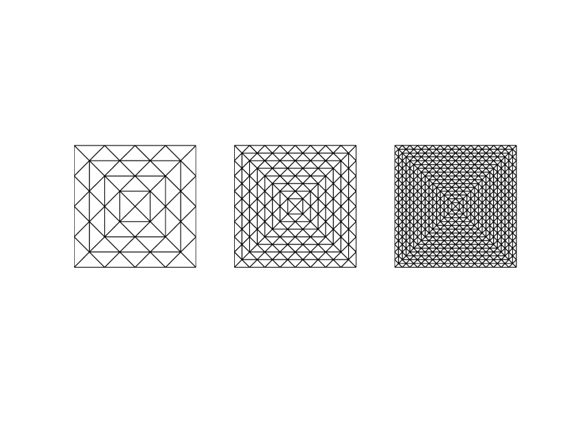
Fig. 3: Structured meshes.

Fig. 4: Unstructured meshes.

7 Complexity issues and perspectives

Lastly, we report some remarks about the computational costs of the proposed iterative procedure by referring to the optimality definition below.  

Definition 10.

[2] Let $\{A_{m}\mathbf{x}_{m}=\mathbf{b}_{m}\}$ be a given sequence of linear systems of increasing dimensions. An iterative method is optimal if

1. the arithmetic cost of each iteration is at most proportional to the complexity of a matrix vector product with matrix $A_{m}$,

2. the number of iterations for reaching the solution within a fixed accuracy can be bounded from above by a constant independent of $m$.

In other words, the problem of solving a linear system with coefficient matrix $A_{m}$ is asymptotically of the same cost as the direct problem of multiplying $A_{m}$ by a vector.

Since we are considering the preconditioning matrix sequence $\{P_{n}(a)\}$ defined as $P_{n}(a)=D_{n}^{{1}/{2}}(a)A_{n}(1,0)D_{n}^{{1}/{2}}(a)$, where $D_{n}(a)=\mathrm{diag}(A_{n}(a,0))\mathrm{diag}\!^{-1}(A_{n}(1,0))$, the solution of the linear system in (5) with matrix $A_{n}(a,\vec{\mathbf{\beta}})$ is reduced to computations involving diagonals and the matrix $A_{n}(1,0)$.
As well known, whenever the domain is partitioned by considering a uniform structured mesh this latter task can be efficiently performed by means of fast Poisson solvers, among which we can list those based on the cyclic reduction idea (see e.g. [8, 10, 25]) and several specialized multigrid methods (see e.g. [13, 18]). Thus, in such a setting, and under the regularity assumptions (3), the optimality of the PHSS method is theoretically proved: the PHSS iterations number for reaching the solution within a fixed accuracy can be bounded from above by a constant independent of the dimension $n=n(h)$ and the arithmetic cost of each iteration is at most proportional to the complexity of a matrix vector product with matrix $A_{n}(a,\vec{\mathbf{\beta}})$.

Finally, we want to stress that the PHSS numerical performances do not get worse in the case of unstructured meshes. In such cases, again, our proposal makes only use of matrix vector products (for sparse or even diagonal matrices) and of a solver for the related diffusion equation with constant coefficient. To this end, the main effort in devising efficient algorithms must be devoted only to this simpler problem.

References

- [1] M. Arioli, E. Noulard, A. Russo, Stopping criteria for iterative methods: applications to PDE’s. Calcolo 38 (2001), no. 2, 97–112.
- [2] O. Axelsson, M. Neytcheva, The algebraic multilevel iteration methods—theory and applications. In Proceedings of the Second International Colloquium on Numerical Analysis (Plovdiv, 1993), 13–23, VSP, 1994.
- [3] Z. Bai, G.H. Golub, M.K. Ng, Hermitian and skew-Hermitian splitting methods for non-Hermitian positive definite linear systems. SIAM J. Matrix Anal. Appl. 24 (2003), no. 3, 603–626.
- [4] B. Beckermann, S. Serra Capizzano, On the Asymptotic Spectrum of Finite Element Matrix Sequences. SIAM J. Numer. Anal. 45 (2007), 746–769.
- [5] D. Bertaccini, G.H. Golub, S. Serra Capizzano, C. Tablino Possio, Preconditioned HSS methods for the solution of non-Hermitian positive definite linear systems and applications to the discrete convection-diffusion equation. Numer. Math. 99 (2005), no. 3, 441–484.
- [6] A. Böttcher, S. Grudsky, On the condition numbers of large semi-definite Toeplitz matrices. Linear Algebra Appl. 279 (1998), 285- 301.
- [7] A. Böttcher, B. Silbermann, Introduction to Large Truncated Toeplitz Matrices. Springer-Verlag, New York, 1998.
- [8] B. Buzbee, F. Dorr, J. George, G.H. Golub, The direct solutions of the discrete Poisson equation on irregular regions. SIAM J. Numer. Anal. 8 (1971), 722- 736.
- [9] L. Cozzi, Analisi spettrale e precondizionamento di discretizzazioni a elementi finiti di equazioni di convezione-diffusione. Master Degree Thesis (in italian), University of Milano Bicocca, Milano, 2006.
- [10] F. Dorr, The direct solution of the discrete Poisson equation on a rectangle. SIAM Rev. 12 (1970), 248- 263.
- [11] J. Jr. Douglas, Alternating direction methods for three space variables, Numer. Math., Vol. 4, pp. 41–63 (1962).
- [12] G.H. Golub, C.F. Van Loan, Matrix computations. Third edition. Johns Hopkins Studies in the Mathematical Sciences. Johns Hopkins University Press, Baltimore, MD, 1996.
- [13] W. Hackbusch, Multigrid Methods and Applications. Springer Verlag, Berlin, Germany, (1985).
- [14] S. Serra Capizzano, Multi-iterative methods, Comput. Math. Appl., 26-4 (1993), pp. 65–87.
- [15] S. Serra Capizzano, On the extreme eigenvalues of Hermitian (block)Toeplitz matrices. Linear Algebra Appl. 270 (1998), 109 -129.
- [16] S. Serra Capizzano, An ergodic theorem for classes of preconditioned matrices. Linear Algebra Appl. 282 (1998), 161- 183.
- [17] S. Serra, The rate of convergence of Toeplitz based PCG methods for second order nonlinear boundary value problems. Numer. Math. 81 (1999), no. 3, 461–495.
- [18] S. Serra Capizzano, Convergence analysis of two grid methods for elliptic Toeplitz and PDEs matrix sequences. Numer. Math. 92-3 (2002), 433 465.
- [19] S. Serra Capizzano, C. Tablino Possio, Spectral and structural analysis of high precision finite difference matrices for elliptic operators. Linear Algebra Appl. 293 (1999), no. 1-3, 85–131.
- [20] S. Serra Capizzano, C. Tablino Possio, High-order finite difference schemes and Toeplitz based preconditioners for elliptic problems. Electron. Trans. Numer. Anal. 11 (2000), 55–84.
- [21] S. Serra Capizzano, C. Tablino Possio, Finite element matrix sequences: the case of rectangular domains. Numer. Algorithms 28 (2001), no. 1-4, 309–327.
- [22] S. Serra Capizzano, C. Tablino Possio, Preconditioning strategies for 2D finite difference matrix sequences. Electron. Trans. Numer. Anal. 16 (2003), 1–29.
- [23] S. Serra Capizzano, C. Tablino Possio, Superlinear preconditioners for finite differences linear systems. SIAM J. Matrix Anal. Appl. 25 (2003), no. 1, 152–164.
- [24] J.R. Shewchuk, A Two-Dimensional Quality Mesh Generator and Delaunay Triangulator. (version 1.6), www.cs.cmu.edu/ quake/triangle.html
- [25] P. Swarztrauber,The method of cyclic reduction, Fourier analysis and the FACR algorithm for the discrete solution of Poisson s equation on a rectangle. SIAM Rev. 19 (1977), 490- 501.
- [26] E.E. Tyrtyshnikov, A unifying approach to some old and new theorems on distribution and clustering. Linear Algebra Appl. 232 (1996), 1–43.