Unity fidelity multiple teleportation using partially entangled states

Abstract

We show that the multiple teleportation protocol (MTP) given in Ref. [Phys. Rev. Lett. 100, 110503 (2008)] is not restricted to the Knill-Laflamme-Milburn (KLM) framework. Rather, we show that MTP can be implemented using any teleportation scheme. We also present two new MTP’s which, under certain situations, are more efficient than the original one, requiring half of the number of its teleportations to achieve at least the same probability of success ($\mathcal{P}_{suc}$). One of the protocols, however, uses less entanglement than the others yielding, surprisingly, the greatest $\mathcal{P}_{suc}$.

I Introduction

The importance of quantum teleportation Ben93 is widely recognized today. Not only does it enable the remote transmission of the state describing a quantum system to another one, without ever knowing the state, but it also allows the construction of a new way to perform quantum computation Got99 ; Kni01 . In the previous and in many other applications of teleportation, it is desirable, if not crucial, that the teleported state arrives at its destination (Bob) exactly as it left the preparation station (Alice). In other words, we want a unity fidelity output state, which is always achieved if Alice and Bob share a maximally entangled state (MES) Ben93 . However, there might happen that our parties do not share a MES or, in addition, intermediate teleportations to other parties must be done before the state reaches Bob. This limitation can be overcome by distilling out of an ensemble of partially entangled states (PES’s) maximally entangled ones Ben96 . But this approach requires a large amount of copies of PES’s to succeed and is ineffective when just a few copies are available. Another way to achieve unity fidelity teleportation with limited resources is based on the probabilistic quantum teleportation (PQT) protocols of Refs. Agr02 ; Gor06 ; Guo00 .

Recently, in an interesting work, Modławska and Grudka Gru08 presented yet another way of achieving probabilistically unity fidelity teleportation. Their strategy was developed in the framework of the KLM scheme Kni01 for linear optical teleportation. The main idea behind their approach was the recognition that multiple (successive) teleportations using the same PES increased the chances of getting a perfect teleported qubit. We can also see the ideas of Ref. Gru08 , as generalized here, as a way to extend the usefulness of quantum relays Bri98 whenever non MES’s are at stake and entanglement concentration is not practical (only a few copies of entangled states are available).

In this contribution we show that the features of the MTP of Ref. Gru08 are not restricted to the KLM teleportation scheme. In order to show that we build in Sec. II a similar protocol (protocol $1$) without relying on the intricacies of the KLM scheme. Actually, we use the same language of the original Bennett et al. proposal Ben93 , which allows us to express $\mathcal{P}_{suc}$, the total probability of getting unity fidelity outcomes, as a function of the number of teleportations and of the shared entanglement between Alice and Bob. We then present two new protocols (protocols $2$ and $3$, see Fig. 1), both of which are more efficient than the previous one. An important feature of these protocols is that they give $\mathcal{P}_{suc}>1/2$ for a huge class of PES’s. This is particularly useful when we have a few copies of the qubit to be teleported, since after a few runs of the MTP the overall $\mathcal{P}_{suc}\rightarrow 1$. On top of that, protocol $2$ possesses the same efficiency of the first one but needs only half the number of teleportations to achieve the same $\mathcal{P}_{suc}$. We also show that this protocol is connected to the PQT of Refs. Agr02 ; Gor06 . Protocol $3$, on the other hand, in addition to requiring just half the number of teleportations of protocol $1$ also achieves the highest $\mathcal{P}_{suc}$. Actually, we show that for some set of PES’s $\mathcal{P}_{suc}\approx 1$ after just a few teleportations within a single run of the MTP. Moreover, and surprisingly, at each successive teleportation this last protocol requires less and less entanglement to properly work. In Sec. III we compare the efficiencies of all the three protocols presented here with a different strategy to achieve unity fiedelity teleportation based on entanglement swapping Bos99 . In particular, we compare our results with those obtained for multiple entanglement swapping as presented in Ref. Per08 . We show that, under certain conditions, we can achieve a better performance using the protocols here presented.

II Multiple teleportation protocols

Protocol 1. Let us assume that we have $j=N$ PES’s described by $|\Phi^{+}_{n_{j}}\rangle=f_{n_{j}}{|00\rangle}+g_{n_{j}}{|11\rangle}$, with $f_{n_{j}}=1/\sqrt{1+n_{j}^{2}}$ and $g_{n_{j}}=n_{j}/\sqrt{1+n_{j}^{2}})$. (See panel (a) of Fig. 1.) We assume the first PES is shared between Alice and Bob while the remaining $N-1$ are with Bob. Without loss of generality we set $0<n_{j}<1$ Gor06 and for this protocol also that $n_{j}=n$, $j=1,\dots,N$ Gru08 , i.e, same entanglement at each teleportation. We can also build a generalized Bell basis as follows,

$${|\Phi_{m_{j}}^{+}\rangle}=f_{m_{j}}{|00\rangle}+g_{m_{j}}{|11\rangle}, {|\Phi_{m_{j}}^{-}\rangle}=g_{m_{j}}{|00\rangle}-f_{m_{j}}{|11\rangle},$$

$${|\Psi_{m_{j}}^{+}\rangle}=f_{m_{j}}{|01\rangle}+g_{m_{j}}{|10\rangle}, {|\Psi_{m_{j}}^{-}\rangle}=g_{m_{j}}{|01\rangle}-f_{m_{j}}{|10\rangle},$$

with $m_{j}=1$ being the original Bell basis and the choice for protocol $1$. Alice wants to teleport the qubit ${|\phi^{A}\rangle}=\alpha{|0\rangle}+\beta{|1\rangle}$ and at each step $j$ a Bell measurement (BM) is implemented whose result is known to Bob (See Fig. 1). This information allows him to correct the final state applying the proper unitary operations conditioned on the results of each BM Ben93 , i.e, $I$ if the BM yields ${|\Phi^{+}\rangle}$, $\sigma_{z}$ for ${|\Phi^{-}\rangle}$, $\sigma_{x}$ for ${|\Psi^{+}\rangle}$, and $\sigma_{z}\sigma_{x}$ for ${|\Psi^{-}\rangle}$, where $I$ is the identity and $\sigma_{z,x}$ the standard Pauli matrices.

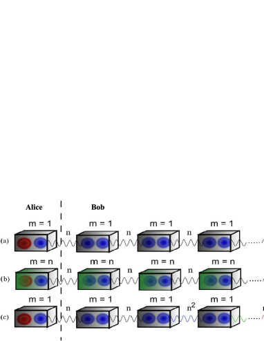
Figure 1: (Color online) Pictorial view of all MTP’s after $q$ teleportations. Note that all but the first PES is shared between Alice and Bob. All the others are at Bob’s. (a) Protocol $1$: Boxes denote standard BM’s ($m=1$) and at each teleportation the quantum channel is the same state ${|\Phi^{+}_{n}\rangle}$. (b) Protocol $2$: Boxes now denote GBM’s with $m=n<1$ with the same state ${|\Phi^{+}_{n}\rangle}$ at each stage. (c) Protocol $3$: Boxes denote standard BM’s ($m=1$) but the quantum channel’s entanglement are successively reduced after the second teleportation according to the following rule, ${|\Phi^{+}_{n_{j}}\rangle}\rightarrow{|\Phi^{+}_{n^{2}_{j}}\rangle}$.

Before the first teleportation the state describing all qubits are ${|\Phi\rangle}={|\phi^{A}\rangle}\otimes_{j=1}^{N}{|\Phi^{+}_{n_{j}}\rangle}$, which can be written as ${|\Phi\rangle}$ $=$ [${|\Phi^{+}\rangle}$ $(f_{1}f_{n}\alpha{|0\rangle}$ $+$ $g_{1}g_{n}\beta{|1\rangle})$ $+$ ${|\Phi^{-}\rangle}$ $\sigma_{z}$ $(g_{1}f_{n}\alpha{|0\rangle}$ $+$ $f_{1}g_{n}\beta{|1\rangle})$ $+$ ${|\Psi^{+}\rangle}$ $\sigma_{x}$ $(f_{1}g_{n}\alpha{|0\rangle}$ $+$ $g_{1}f_{n}\beta{|1\rangle})$ $+$ ${|\Psi^{-}\rangle}$ $\sigma_{z}\sigma_{x}$ $(g_{1}g_{n}\alpha{|0\rangle}$ $+$ $f_{1}f_{n}\beta{|1\rangle})]$ $\otimes_{j=2}^{N}{|\Phi^{+}_{n_{j}}\rangle}.$ Unity fidelity teleportation occurs only if $f_{1}f_{n}=g_{1}g_{n}$ or $f_{1}g_{n}=g_{1}f_{n}$. But this is only possible if we have a MES ($n=1$ $\rightarrow$ $f_{n}=f_{1}=g_{n}=g_{1}=1/\sqrt{2}$). Hence, after the first teleportation $P^{(1)}_{suc}=0$. It is important to note that at each teleportation, the previous teleported qubit is changed to $\alpha_{j-1}\rightarrow\alpha_{j}=h_{j}^{\alpha}\alpha_{j-1}$ and $\beta_{j-1}\rightarrow\beta_{j}=h_{j}^{\beta}\beta_{j-1}$, with $(h_{j}^{\alpha},h_{j}^{\beta})$ $=$ $(f_{1}f_{n},g_{1}g_{n})$, or $(g_{1}f_{n},f_{1}g_{n})$, or $(f_{1}g_{n},g_{1}f_{n})$, or $(g_{1}g_{n},f_{1}f_{n})$, for $j>1$ and $\alpha_{0}=\alpha$ and $\beta_{0}=\beta$. We are neglecting normalization for the moment. After the second teleportation there exist $16$ possible outcomes ($4\times 4$ pairs of BM’s) for the teleported qubit, which is described by one of $16$ states whose coefficients are given by terms like $(\alpha_{2},\beta_{2})$ $=$ $(h_{2}^{\alpha}\alpha_{1},h_{2}^{\beta}\beta_{1})$ $=$ $(f_{1}f_{n}f_{1}f_{n}\alpha,g_{1}g_{n}g_{1}g_{n}\beta)$, $(g_{1}f_{n}f_{1}f_{n}\alpha,f_{1}g_{n}g_{1}g_{n}\beta)$, $\dots$, $(g_{1}g_{n}g_{1}g_{n}\alpha,f_{1}f_{n}f_{1}f_{n}\beta)$. Of all possibilities, those giving unity fidelity are such that $h_{2}^{\alpha}=h_{2}^{\beta}$, since we can factor out the terms multiplying $\alpha$ and $\beta$ obtaining the exact original state $|\phi^{A}\rangle$. To determine those successful cases we first note that whenever ${|\Phi^{\pm}\rangle}$ is a result of a BM the teleported coefficients change to $\alpha_{j}\rightarrow\alpha_{j}$ with $\beta_{j}\rightarrow n\beta_{j}$. Second, whenever the BM results in ${|\Psi^{\pm}\rangle}$ we get $\alpha_{j}\rightarrow n\alpha_{j}$ and $\beta_{j}\rightarrow\beta_{j}$. Therefore, it is not difficult to see that we always get unity fidelity teleportation when we have an equal number of $|\Phi^{\pm}\rangle$ and ${|\Psi^{\pm}\rangle}$ in a sequence of BM’s, or equivalently, an equal number of functions $g_{n}$ multiplying $\alpha$ and $\beta$. For the case of two teleportations the successful cases are given by eight possibilities: ${|\Phi^{\pm}\rangle}{|\Psi^{\pm}\rangle}$ and ${|\Psi^{\pm}\rangle}{|\Phi^{\pm}\rangle}$. The probability of all those cases are equal and is given by $P_{event}^{(2)}$ $=$ $n^{2}/[4(1+n^{2})^{2}]$. Thus, $P_{suc}^{(2)}=2n^{2}/(1+n^{2})^{2}$. If we are successful, we do not need another teleportation. However, if we fail, we need to proceed with successive teleportations, hoping to get a balanced sequence of $|\Phi^{\pm}\rangle$ and ${|\Psi^{\pm}\rangle}$ BM’s. We can show that at the $q$-th teleportation

$$P_{suc}^{(q)}=A(q)n^{q}/[2^{q}(1+n^{2})^{q}],$$ (1)

where for $q$ odd $A(q)=0$ and for $q$ even A(q) is the number of all possible combinations of $q$ BM’s in which we have an equal number of $|\Phi^{\pm}\rangle$ and $|\Psi^{\pm}\rangle$, excluding, of course, those cases where we already had a balanced number in the previous even teleportations. For the first $12$ teleportations we have $A(2)=8$, $A(4)=32$, $A(6)=256$, $A(8)=2560$, $A(10)=28672$, and $A(12)=344064$. In Fig. 2 we plot the total probability of success after the $q$-th teleportation, $\mathcal{P}_{suc}=\sum_{j=1}^{q}P_{suc}^{(j)},$ as a function of $n$ (the greater $n$ the greater the entanglement). Note that here and in the remaining of this section $\mathcal{P}_{suc}$ is given by the sum of the probabilities of all previous successful teleportations since the $N-1$ PES’s are with Bob. In Sec. III we also study other scenarios, in particular the one in which Bob possesses just one PES.

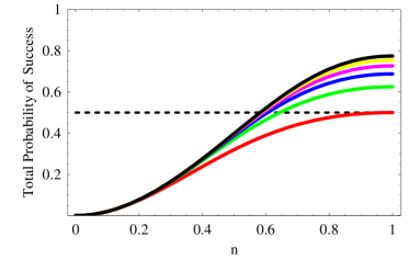
Figure 2: (Color online) For protocol 1: From bottom to top the curves represent $\mathcal{P}_{suc}$ after $q=2$, $4$, $6$, $8$, $10$, and $12$ successive teleportations. For protocol 2: From bottom to top the curves show $\mathcal{P}_{suc}$ after $q=1$, $2$, $3$, $4$, $5$, and $6$ successive teleportations. The dashed curve shows the optimal probability (1/2) using the PQT protocol. All quantities are dimensionless.

Looking at Fig. 2 we see that after each teleportation $\mathcal{P}_{suc}$ increases at a lower rate. Also, after the $10$-th teleportation we are already close to the maximal value of $\mathcal{P}_{suc}$ for whatever value of $n$. We should remark that we are considering success only unity fidelity teleportations. That is why $\mathcal{P}_{suc}$ does not tend to one as $n\rightarrow 1$. Indeed, no matter how close $n$ is to one we are always discarding the sequences of BM’s where we do not get a balanced set of measurements involving the Bell states $|\Phi^{\pm}\rangle$ and $|\Psi^{\pm}\rangle$.

Protocol 2. As before, we assume that one has $j=N$ PES’s described by $|\Phi^{+}_{n_{j}}\rangle$, with $0<n_{j}<1$ and $n_{j}=n$, $j=1,\dots,N$. (See panel (b) of Fig. 1.) However, differently from protocol $1$, we now assume $m_{j}=m=n$, any $j$. The state to be teleported is ${|\phi^{A}\rangle}=\alpha{|0\rangle}+\beta{|1\rangle}$ and at each step $j$ one implements a generalized Bell measurement (GBM) Agr02 ; Gor06 . A GBM is a projective measurement of two qubits onto one of the four generalized Bell states given above (See Ref. Kim04 for ways of implementing a GBM.) The result of each GBM is known to Bob who uses this information to apply the right unitary operations on his qubit as described in the first protocol. The rest of the present protocol is nearly the same as before and is inspired by the PQT of Refs. Agr02 ; Gor06 .

Before any teleportation the state describing all qubits can be written as ${|\Phi\rangle}$ $=$ [${|\Phi^{+}_{m}\rangle}$ $(f_{m}f_{n}\alpha{|0\rangle}$ $+$ $g_{m}g_{n}\beta{|1\rangle})$ $+$ ${|\Phi^{-}_{m}\rangle}$ $\sigma_{z}$ $(g_{m}f_{n}\alpha{|0\rangle}$ $+$ $f_{m}g_{n}\beta{|1\rangle})$ $+$ ${|\Psi^{+}_{m}\rangle}$ $\sigma_{x}$ $(f_{m}g_{n}\alpha{|0\rangle}$ $+$ $g_{m}f_{n}\beta{|1\rangle})$ $+$ ${|\Psi^{-}_{m}\rangle}$ $\sigma_{z}\sigma_{x}$ $(g_{m}g_{n}\alpha{|0\rangle}$ $+$ $f_{m}f_{n}\beta{|1\rangle})]$ $\otimes_{j=2}^{N}{|\Phi^{+}_{n_{j}}\rangle}.$ Note that now we have rewritten the first two qubits using the generalized Bell basis with $m=n$, i.e., we have imposed the ‘matching condition’, where the entanglement of the channel and of the measuring basis are the same Agr02 ; Gor06 . This allows us to obtain unity fidelity teleportation right after the first teleportation whenever we measure $|\Phi^{-}_{m}\rangle$ or $|\Psi^{+}_{m}\rangle$ with $P^{(1)}_{suc}=2n^{2}/(1+n^{2})^{2}$. The previous step is precisely the PQT Agr02 ; Gor06 . To analyze the other teleportations we need to keep in mind three facts. (1) The $j$-th teleported qubit is changed to $(\alpha_{j},\beta_{j})\rightarrow(\alpha_{j},n^{2}\beta_{j})$ whenever ${|\Phi^{+}_{m}\rangle}$ is a result of a GBM; (2) If the GBM yields ${|\Phi^{-}_{m}\rangle}$ or ${|\Psi^{+}_{m}\rangle}$ we get $(\alpha_{j},\beta_{j})\rightarrow n(\alpha_{j},\beta_{j})$; (3) if we measure ${|\Psi^{-}_{m}\rangle}$ the qubit goes to $(\alpha_{j},\beta_{j})\rightarrow(n^{2}\alpha_{j},\beta_{j})$. Therefore, when we have an equal number of $|\Phi^{+}_{m}\rangle$ and ${|\Psi^{-}_{m}\rangle}$, $m=n$, in a sequence of GBM’s we get unity fidelity. The $n^{2}\beta_{j}$ coming from the measurement of $|\Phi^{+}_{m}\rangle$ is compensated by the $n^{2}\alpha_{j}$ coming from another GBM giving ${|\Psi^{-}_{m}\rangle}$. Note that the states ${|\Phi^{-}_{m}\rangle}$ and ${|\Psi^{+}_{m}\rangle}$ are ‘neutral’, giving an overall $n$ that can be ignored for the determination of the successful cases. For example, after the second teleportation we have two possible GBM outcomes where we have a unity fidelity teleportation, namely, ${|\Phi^{+}_{m}\rangle}{|\Psi^{-}_{m}\rangle}$ and ${|\Psi^{-}_{m}\rangle}{|\Phi^{+}_{m}\rangle}$ with $P^{(2)}_{suc}=2n^{4}/(1+n^{2})^{4}$. And after the third teleportation the successful cases are four: ${|\Phi^{+}_{m}\rangle}{|\Phi^{-}_{m}\rangle}{|\Psi^{-}_{m}\rangle}$, ${|\Phi^{+}_{m}\rangle}{|\Psi^{+}_{m}\rangle}{|\Psi^{-}_{m}\rangle}$, ${|\Psi^{-}_{m}\rangle}{|\Phi^{-}_{m}\rangle}{|\Phi^{+}_{m}\rangle}$, and ${|\Psi^{-}_{m}\rangle}{|\Psi^{+}_{m}\rangle}{|\Phi^{+}_{m}\rangle}$, with $P^{(3)}_{suc}=4n^{6}/(1+n^{2})^{6}$. In general, after the $q$-th teleportation we have,

$$P_{suc}^{(q)}=B(q)n^{2q}/[(1+n^{2})^{2q}],$$ (2)

where B(q) is the number of all possible combinations of $q$ GBM’s where we have an equal number of $|\Phi^{+}_{m}\rangle$ and $|\Psi^{-}_{m}\rangle$, excluding, as we did in protocol $1$, the cases where we already got an equal number of those two states in the previous teleportations. For the first six teleportations we have $B(1)=2$, $B(2)=2$, $B(3)=4$, $B(4)=10$, $B(5)=28$, and $B(6)=84$.

Noting that $A(2q)/2^{2q}=B(q)$ we immediately see that Eqs. (1) and (2) are the same. However, in protocol $2$, we just need half of the number of teleportations to achieve the same efficiency, which is a quite remarkable economy on entanglement resources. Also, the need for less teleportations reduces other possible errors introduced by imperfect projective measurements. Furthermore, this result connects the PQT of Refs. Agr02 ; Gor06 to protocol $1$. This is true because two successive teleportations using that protocol is equivalent to one using protocol $2$, being the latter an extension of the PQT.

Protocol 3. Like protocol $1$, here we do not need GBM’s. (See panel (c) of Fig. 1.) The projective measurements are made using the standard Bell basis, i.e., $m_{j}=1$, any $j$. However, and differently from the previous protocols, we assume that at each teleportation the entanglement of the quantum channel is reduced according to the following rule: $n_{j}=n_{j-1}^{2}$, $j\geq 3$ with $n_{1}=n_{2}=n<1$. In words, the first two teleportations are done spending two entangled states $|\Phi^{+}_{n}\rangle$ and after that we start using less and less entanglement. The first two steps of this protocol are identical to the first two of protocol $1$ yielding $P_{suc}^{(1)}=0$ and $P_{suc}^{(2)}=2n^{2}/(1+n^{2})^{2}$. After the second teleportation, the unsuccessful cases are described by the state $\alpha{|0\rangle}+n^{2}\beta{|1\rangle}$, if the BM’s resulted in $|\Phi^{\pm}\rangle|\Phi^{\pm}\rangle$, or by the state $n^{2}\alpha{|0\rangle}+\beta{|1\rangle}$, if the two successive BM’s yielded $|\Psi^{\pm}\rangle|\Psi^{\pm}\rangle$. Since in the third teleportation the entangled state spent is ${|\Phi^{+}_{n^{2}}\rangle}$, the previous teleported qubit changes to $(\alpha_{2},\beta_{2})\rightarrow(\alpha_{2},n^{2}\beta_{2})$ if we measure $|\Phi^{\pm}\rangle$ or to $(\alpha_{2},\beta_{2})\rightarrow(n^{2}\alpha_{2},\beta_{2})$ if we get $|\Psi^{\pm}\rangle$. Hence, whenever we get the following sequences of BM’s, $|\Phi^{\pm}\rangle|\Phi^{\pm}\rangle|\Psi^{\pm}\rangle$ or $|\Psi^{\pm}\rangle|\Psi^{\pm}\rangle|\Phi^{\pm}\rangle$ we achieve unity fidelity with $P_{suc}^{(3)}=2n^{4}/[(1+n^{2})^{2}(1+n^{4})]$. The unsuccessful cases are given by the following $16$ cases, $|\Phi^{\pm}\rangle|\Phi^{\pm}\rangle|\Phi^{\pm}\rangle$ and $|\Psi^{\pm}\rangle|\Psi^{\pm}\rangle|\Psi^{\pm}\rangle$, with the unsuccessful teleported qubits being either $(\alpha,n^{4}\beta)$ or $(n^{4}\alpha,\beta)$, respectively.

It is now clear why we will use ${|\Phi^{+}_{n^{4}}\rangle}$ to implement the fourth teleportation. We are trying to catch up with the $n^{4}$ that multiplies either $\alpha$ or $\beta$. And since the unsuccessful cases after this step will turn to have a $n^{8}$ multiplying either $\alpha$ or $\beta$, we will need ${|\Phi^{+}_{n^{8}}\rangle}$ at the fifth teleportation to catch up with it. In general, after the $(q-1)$-th teleportation the unsuccessful cases are those where we got the following sequences of $q-1$ BM’s: $\otimes_{j=1}^{q-1}{|\Phi^{\pm}\rangle}$ or $\otimes_{j=1}^{q-1}{|\Psi^{\pm}\rangle}$, giving a total of $2\times 2^{q-1}$ cases with unsuccessful (not normalized) teleported qubits described by $\alpha{|0\rangle}+n^{2^{q-2}}\beta{|1\rangle}$ or $n^{2^{q-2}}\alpha{|0\rangle}+\beta{|1\rangle}$, respectively. At the $q$-th teleportation we succeed if we have either $(\otimes_{j=1}^{q-1}{|\Phi^{\pm}\rangle}){|\Psi^{\pm}\rangle}$ or $(\otimes_{j=1}^{q-1}{|\Psi^{\pm}\rangle}){|\Phi^{\pm}\rangle}$ as our sequence of BM’s, with the probability to get any single successful sequence being identical and given by $P_{event}^{(q)}=n^{2^{q-1}}/[2^{q}(1+n^{2})\prod_{j=1}^{q-1}(1+n^{2^{j}})]$. But since we have a total of $2\times 2^{q}$ successful sequences we get ($q\geq 2$),

$$P_{suc}^{(q)}=2n^{2^{q-1}}(1-n^{2})/[(1+n^{2})(1-n^{2^{\,\!{}^{q}}})],$$ (3)

where we used that $\prod_{j=1}^{q-1}(1+n^{2^{j}})=(1-n^{2^{q}})/(1-n^{2})$. There is also a peculiar way of writing $P_{suc}^{(q)}$ in terms of the concurrence Woo98 , $C_{n_{j}}=2n_{j}/(1+n_{j}^{2})$, an entanglement monotone/quantifier for the state $|\Phi^{+}_{n_{j}}\rangle$,

$$P_{suc}^{(q)}=2\mbox{$\prod_{j=1}^{q}$}C_{n_{j}}/2,\hskip 28.45274ptq\geq 2.$$

Actually, for the other two protocols we can write similar expressions for $P_{suc}^{(q)}$. The difference comes from the factor multiplying the product of concurrences. Here, this factor is $2$, for the other protocols, they are $A(q)/2^{q}$ and $B(q)$. In protocol $2$ we must also consider the concurrences of the GBM. This changes, in the above expression for $P^{(q)}_{suc}$, the term $C_{n_{j}}/2$ to $C_{n_{j}}C_{m_{j}}/4$.

In Fig. 3 we plot the total probability of success after $q$ teleportations, $\mathcal{P}_{suc}=\sum_{j=1}^{q}P_{suc}^{(j)}$, as a function of $n$.

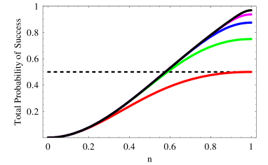
Figure 3: (Color online) From bottom to top the curves show $\mathcal{P}_{suc}$ after $q=2$, $3$, $4$, $5$, and $6$ successive teleportations using protocol $3$. The dashed curve shows the optimal probability (1/2) obtained using the PQT protocol.

Comparing Fig. 2 with Fig. 3 we see that protocol $3$ is far better than the previous two by any aspect we might consider. First, it achieves the greatest $\mathcal{P}_{suc}$. Indeed, for values of $n\approx 0.9$ we can get $\mathcal{P}_{suc}\approx 0.9$, a feat unattainable by the previous protocols. Second, it achieves its maximum $\mathcal{P}_{suc}$ using half the teleportations of protocol $1$. Third, it uses much less entanglement to achieve those highest $\mathcal{P}_{suc}$ since after the second teleportation the entangled states employed change from ${|\Phi^{+}_{n_{j}}\rangle}$ to ${|\Phi^{+}_{n_{j}^{2}}\rangle}$. This last result is really remarkable and surprising. It means that in the framework of MTP less entanglement at each step of the protocol is more useful to achieve a higher $\mathcal{P}_{suc}$ than keeping the same degree of entanglement for the quantum channel. Also, since entanglement is a precious and difficult resource to obtain, this property of the MTP can be really useful in practical applications. It is worth mentioning that one interesting question remains to be answered. Is this protocol the optimal one? For just a few teleportations a partial analysis suggest that protocol $3$ may be the optimal one. However, no general proof, even numerically, is available yet.

There is another property which is also existent in the previous two protocols. Looking at $\mathcal{P}_{suc}$ as a function of the number of teleportations we see it achieves its maximal value after a small number of steps. This is more evident the lower the entanglement of the quantum channel. Looking at Fig. 3 we see that for $n<0.6$ just three teleportations are enough to achieve the maximal $\mathcal{P}_{suc}$. And for higher values of $n$, a few more give the same feature. This is a practical property of MTP for we do not need to implement a prohibitively large number of teleportations to get the optimal value of $\mathcal{P}_{suc}$. One last remark. We can also look at protocol $3$ as a way to correct errors in previous teleportations. If it is discovered that in a previous step of the protocol an error changed the entangled state used in the teleportation process we can correct it by properly choosing the right entangled state for the next teleportation.

III Comparison with multiple entanglement swapping

So far we have considered a “direct approach” to teleport a qubit using PES’s. By direct we mean that we use the PES’s as they are offered to us, without any pre-processing. We have also assumed that Bob has access to $N-1$ PES’s out of a total of $N$. But we can change this scenario in at least two ways. On the one hand we can impose that Bob has access to only one PES. The other $N-2$ states lie between Alice and Bob. See the bottom of Fig. 4. On the other hand we can first try to extract a maximally entangled state out of those $N$ PES’s and only then implement the usual, single-shot, teleportation protocol. See the top-left of Fig. 4, for example. Our goal in this section is to compare the efficiencies (probabilities of success) for the present direct protocols with the ones achieved using the multiple entanglement swapping protocol (“swapping approach”) of Ref. Per08 , whose goal is to obtain out of $N$ PES’s linking Alice and Bob (bottom of Fig. 4, for example) one maximally entangled state (a Bell state). In this “indirect approach”, a sequence of $N-1$ joint measurements (not only Bell measurements) are implemented on qubits from different entangled states (solid rectangles of Fig. 4), with the hope that at the end of the protocol the two qubits at end of the chain become entangled. These measurements are chosen in such a way to maximize the probability of Alice and Bob getting a maximally entangled two-qubit state (Bell state) at the end of the protocol. It is this Bell state that afterwards is employed to teleport the qubit with Alice to Bob. As will be shown, we achieve the highest probability of success (unity fidelity teleportation) sometimes using the direct or the swapping approach. The best strategy is dictated by the degree of entanglement of the PES’s and also by the way they are distributed between Alice and Bob.

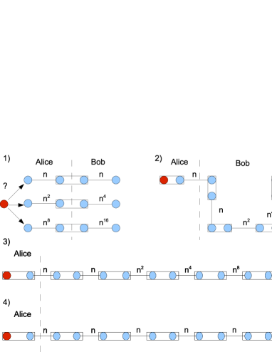
Figure 4: (Color online) (1), (2), and (3) show three possible configurations involving six PES’s with decreasing entanglement while (4) shows configuration (3) with six PES’s possessing the same entanglement. The dashed vertical lines delimitate which qubits Alice and Bob have access to, the solid line rectangles represent Bell measurements, and solid lines mean entanglement between the connected qubits.

We start our analysis comparing the total probability of success for protocols $2$ and $3$ against the total probability of success for the swapping approach as giving by Eq. $D3$ of Ref. Per08 , the best strategy for multiple swapping teleportation. Equation $D3$ gives the probability ($P_{swap}$) of getting one maximally entangled state out of $N$ PES’s, which can then be used to implement the usual teleportation scheme. To derive Eq. $D3$ it is assumed that all PES’s have the same entanglement and that Alice and Bob have access to only one PES, as depicted at the bottom of Fig. 4. In the present notation, Eq. $D3$ reads

$$P_{swap}=1-(f_{n}^{2}-g_{n}^{2})\sum_{j=0}^{[N/2]}f_{n}^{2j}g_{n}^{2j}\left(\begin{array}[]{c}2j\\ j\end{array}\right),$$

with $[N/2]$ denoting the integer part of $N/2$, $\left(\begin{array}[]{c}2j\\ j\end{array}\right)$ meaning the binomial coefficient, $f_{n}=1/\sqrt{1+n^{2}}$, and $g_{n}=n/\sqrt{1+n^{2}}$.

In our first analysis we consider for protocols $2$ and $3$ that the $N-1$ PES’s are with Bob. For protocol $2$ they all have the same entanglement while for protocol $3$ the entanglement decreases as explained in the previous section. (See top-right of Fig. 4.) Note that for protocol $2$ we have generalized Bell measurements. For the swapping approach, we consider the configuration given at the bottom of Fig. 4. The results for this scenario are illustrated in Fig. 5, where we plot the probabilities of success for $N=6$ PES’s. Note that in this situation, protocols $2$ or $3$ are superior for almost all the range of the parameter $n$.

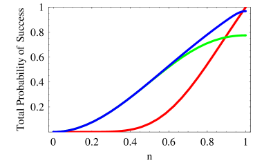
Figure 5: (Color online) Upper curves represent in ascending order $\mathcal{P}_{suc}$ for protocols $2$ (green) and $3$ (blue) in configuration $(2)$ of Fig. 4. The bottom curve (red) gives $\mathcal{P}_{suc}$ for the swapping approach at configuration $(4)$ of Fig. 4. See text for more details.

We now compare the swapping approach as given by configuration $(1)$ of Fig. 4, the optimal way for a swapping-based protocol, with protocol $3$ as given by configuration $(2)$ of Fig. 4. Since we have three chances (three pairs of PES’s) for succeeding, we get for the swapping protocol $\mathcal{P}_{suc}=S_{1}+(1-S_{1})S_{2}+(1-S_{1})(1-S_{2})S_{3}$. Here $S_{j}$, $j=1,2,3$, gives the optimal probability to obtain a maximally entangled state out of two pairs of PES’s. One can show that Per08 $S_{j}=2n_{j}^{2}/(1+n_{j}^{2})$, with $n_{1}=n$, $n_{2}=n^{4}$, and $n_{3}=n^{16}$. Looking at Fig. 6 we see that in this case the swapping protocol is slightly superior for $n\stackrel{{\scriptstyle>}}{{\sim}}0.6$ while for small $n$ they both give the same efficiencies. We should also mention that if all the six pairs of PES’s are shared between Alice and Bob, a complete different scenario from the ones depicted in Fig. 4, entanglement concentration/filtering techniques applied individually to all the six pairs Vid99 give a better performance. This is true because the optimal probability to locally concentrate a maximally entangled state from a non-maximally pure one is $P_{con}=S_{j}$ Vid99 . However, entanglement concentration can only be applied if Alice and Bob initially do share entangled states. In the majority of the situations studied here, though, Alice and Bob do not initially share any entangled state and we have no choice but to rely on the multiple teleportation or on the multiple swapping techniques.

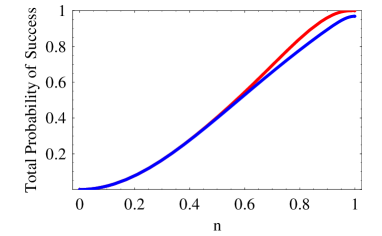
Figure 6: (Color online) The upper/red curve represents $\mathcal{P}_{suc}$ for the swapping protocol in the configuration (1) of Fig. 4 and the lower/blue one $\mathcal{P}_{suc}$ for protocol $3$ at configuration (2) of Fig. 4.

We end this section comparing both approaches at the same configuration, namely, configuration (4) of Fig. 4. For the direct approach we employ protocol $1$. In this scenario $\mathcal{P}_{suc}$ for the swapping approach is given by Eq. $D3$ of Ref. Per08 , where we assume all PES’s to be described by the state $|\Phi^{+}_{n}\rangle$. For protocol $1$ $\mathcal{P}_{suc}$ is calculated considering only those instances in which the qubit arrives with unity fidelity at its final destination. This always happens whenever the Bell measurements after the six teleportations yield a balanced number of $|\Phi^{\pm}\rangle$ and $|\Psi^{\pm}\rangle$. A simple numerical count gives $1280$ possible ways that this can happen with the total probability being $\mathcal{P}_{suc}=20n^{6}/(1+n^{2})^{6}$. Fig. 7 shows $\mathcal{P}_{suc}$ for both approaches when we have six PES’s. It is interesting to note that for $n<0.557$ the direct approach is the best choice. We have numerically checked that the lower the number of PES’s the greater the value of $n$ below which the direct approach is the best choice. For more than $10$ PES’s the swapping protocol can be considered the best choice.

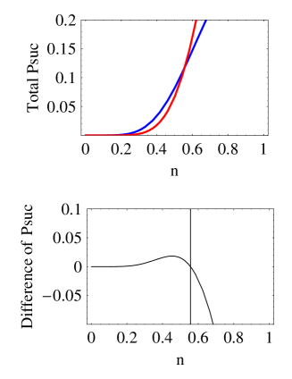
Figure 7: (Color online) Top: For small values of $n$, the upper/blue curve represents $\mathcal{P}_{suc}$ for protocol 1 while the bottom/red curve $\mathcal{P}_{suc}$ for the swapping approach. Both cases are analyzed at configuration (4) of Fig. 4. Bottom: The vertical line (n=0.557) marks the critical value below which the direct approach yields a better performance.

Finally, we have compared the efficiency of protocol $1$ in configuration (4) of Fig. 4 against protocol $3$ in configuration (3). We always obtained better results for protocol $1$ in this case.

IV Conclusion

We have shown that the properties of the multiple teleportation protocol (MTP) are a general feature of successive teleportations, not being restricted to the Knill-Laflamme-Milburn (KLM) scheme. We have also connected one formulation of MTP to the probabilistic quantum teleportation (PQT), another approach that aims to achieve unity fidelity teleportation via partially entangled states (PES’s). Moreover, we have presented two new MTP’s that are more efficient than the original one. Indeed, in those two new MTP’s we just need half the number of teleportations of the original MTP to achieve at least the same probability of success (unity fidelity teleportation). On top of that, we have shown that the protocol furnishing the highest probability of success (protocol $3$) is the one requiring, surprisingly, the least amount of entanglement for its full implementation. On the one hand, this result may have important practical applications, since it is known that entanglement is a difficult resource to produce experimentally, and, on the other hand, it suggests that whenever PES’s are at stake, perhaps the best strategy to achieve a certain goal is not the one that uses the greatest amount of entanglement. Finally, we have compared the three MTP’s here developed with the multiple entanglement swapping approach developed in Ref. Per08 . We have checked that either one or the other approach furnished a better performance, depending on the amount of entanglement available and on the way the PES’s are distributed between Alice and Bob.

- (1) C. H. Bennett et al., Phys. Rev. Lett. 70, 1895 (1993).
- (2) D. Gottesman and I. L. Chuang, Nature (London) 402, 390 (1999).
- (3) E. Knill R. Laflamme, and G. J. Milburn, Nature (London) 409, 46 (2001).
- (4) C. H. Bennett et al., Phys. Rev. Lett. 76, 722 (1996).
- (5) P. Agrawal and A. K. Pati, Phys. Lett. A 305, 12 (2002).
- (6) G. Gordon and G. Rigolin, Phys. Rev. A 73, 042309 (2006).
- (7) W.-Li Li, C.-Feng Li, and G.-C. Guo, Phys. Rev. A 61, 034301 (2000).
- (8) J. Modławska and A. Grudka, Phys. Rev. Lett. 100, 110503 (2008).
- (9) H.-J. Briegel et al., Phys. Rev. Lett. 81, 5932 (1998).
- (10) S. Bose, V. Vedral, and P. L. Knight, Phys. Rev. A 60, 194 (1999).
- (11) S. Perseguers et al., Phys. Rev. A 77, 022308 (2008).
- (12) H. Kim, Y.W. Cheong, H.W. Lee, Phys. Rev. A 70, 012309 (2004).
- (13) G. Vidal, Phys. Rev. Lett. 83, 1046 (1999).
- (14) W. K. Wootters, Phys. Rev. Lett. 80, 2245 (1998).