An MHD Gadget for cosmological simulations

Abstract

Various radio observations have shown that the hot atmospheres of galaxy clusters are magnetized. However, our understanding of the origin of these magnetic fields, their implications on structure formation and their interplay with the dynamics of the cluster atmosphere, especially in the centers of galaxy clusters, is still very limited. In preparation for the upcoming new generation of radio telescopes (like EVLA, LWA, LOFAR and SKA), a huge effort is being made to learn more about cosmological magnetic fields from the observational perspective. Here we present the implementation of magneto-hydrodynamics in the cosmological SPH code GADGET (Springel et al., 2001; Springel, 2005). We discuss the details of the implementation and various schemes to suppress numerical instabilities as well as regularization schemes, in the context of cosmological simulations. The performance of the SPH-MHD code is demonstrated in various one and two dimensional test problems, which we performed with a fully, three dimensional setup to test the code under realistic circumstances. Comparing solutions obtained using ATHENA (Stone et al., 2008), we find excellent agreement with our SPH-MHD implementation. Finally we apply our SPH-MHD implementation to galaxy cluster formation within a large, cosmological box. Performing a resolution study we demonstrate the robustness of the predicted shape of the magnetic field profiles in galaxy clusters, which is in good agreement with previous studies.

1 Introduction

Magnetic fields have been detected in galaxy clusters by radio observations, via the Faraday Rotation Signal of the magnetized cluster atmosphere towards polarized radio sources in or behind clusters (see Carilli & Taylor, 2002; Govoni & Feretti, 2004, for recent reviews) and from diffuse synchrotron emission of the cluster atmosphere (see Govoni & Feretti, 2004; Ferrari et al., 2008, for recent reviews). Our understanding of the origin of cosmological magnetic fields is particularly limited. But their evolution and possible implications for structure formation are also not yet fully understood. In addition their interplay with the large-scale structure formation processes, as well as their link to additional dynamics within the cluster atmosphere is unclear, especially their role in the cool core regions and the influence of these regions on the evolution of the magnetic fields.

The upcoming, new generation of radio telescopes (like EVLA, LWA, LOFAR and SKA) will dramatically increase the volume of observational data relevant for our understanding of cosmological seed magnetic fields in the near future. To investigate the general characteristics of the magnetic fields in and beyond galaxy clusters at the level required for a meaningful comparison to current and forthcoming observations, numerical simulations are mandatory. Non-radiative simulations of galaxy clusters within a cosmological environment which follow the evolution of a primordial magnetic seed field have been performed using Smooth-Particle-Hydrodynamics (SPH) codes (Dolag et al., 1999, 2002; Dolag et al., 2005) as well as Adaptive Mesh Refinement (AMR) codes (Brüggen et al., 2005; Dubois & Teyssier, 2008). Although these simulations are based on quite different numerical techniques they show good agreement in the predicted properties of the magnetic fields in galaxy clusters. When radiative cooling is included, strong amplification of the magnetic fields inside the cool-core region of clusters is found (Dubois & Teyssier, 2008), in good agreement with previous work (Dolag, 2000). Cosmological, magneto-hydrodynamical simulations were also performed using finite-volume and finite-difference methods. Such simulations are used to either follow a primordial magnetic field (Li et al., 2008) or the creation of magnetic fields in shocks through the so-called Biermann battery effect (Kulsrud et al., 1997; Ryu et al., 1998), on which a subsequent turbulent dynamo may operate. The latter predict magnetic field strength in filaments with somewhat higher values (e.g. see Sigl et al., 2004) than predicted by simulations which start from a primordial magnetic seed field, but are in line with predictions of magnetic field values from turbulence (Ryu et al., 2008). Therefore further investigations are needed to clarify the structure, evolution and origin of magnetic fields in the largest structures of the Universe, their observational signatures, as well as their interplay with other processes acting in galaxy clusters and the large scale structure.

The complexity of galaxy clusters comes principly from their hierarchical build up within the large-scale structure of the Universe. In order to study their formation it is necessary, to follow a large volume of the Universe. However, one must also describe cosmic structures down to relatively small scales, thus spanning 5 to 6 orders of magnitudes in size. The complexity of the cluster atmosphere reflects the infall of thousands of smaller objects and their subsequent destruction or survival within the cluster potential. Being the source of shocks and turbulence, these processes directly act on the magnetic field causing re-distribution and amplification. Therefore realistic modelling of these processes critically depends on the ability of the simulation to resolve and follow correctly this dynamics in galaxy clusters.

Starting from a well-established cosmological n-body smoothed particle hydrodynamic (SPH) code GADGET (Springel et al., 2001; Springel, 2005) we present here the implementation of magneto-hydrodynamics, which allows us to explore the full size and dynamical range of state of the art cosmological simulations. GADGET also allows us to turn on the treatment of many additional physical processes which are of interest for structure formation and make interesting links with the treatment of magnetic fields for future studies. This includes thermal conduction (Jubelgas et al., 2004; Dolag et al., 2004), physical viscosity (Sijacki & Springel, 2006), cooling and star-formation (Springel & Hernquist, 2003), detailed modelling of the stellar population and chemical enrichment (Tornatore et al., 2004, 2007) and a self consistent treatment of cosmic rays (Enßlin et al., 2007; Pfrommer et al., 2007). The MHD implementation presented here is fully compatible with all these extensions, but here we want to focus on non-radiative simulations. All such processes are expected to increased the complexity and lead to interplay with the evolution of the magnetic field. This would make it impossible to critically check the numerical effects caused by the different SPH-MHD implementations and therefore we will ignore such additional processes in this work.

The paper is structured as follows: In section 2 we present the details of the numerical implementation, whereas in section 3 we present various code validation tests, all performed in fully three dimensional setups. In section 4 we present the formation of a galaxy cluster as an example for a cosmological application before we present our conclusions in section 5. In addition we present a convergence test for the code in the appendix.

2 SPH-MHD Implementation

We have implemented the MHD equations in the cosmological SPH code GADGET (Springel et al., 2001; Springel, 2005). In this section we present the relevant details of this implementation. While developing the MHD implementation made use of GADGET-1 (Springel et al., 2001) and GADGET-2 (Springel, 2005), all simulations presented in this paper are based on the most recent version of the code, GADGET-3 (Springel, in prep). Note that the implementation therefore is fully parallelized and benefits from many optimizations within the general parts of the code, especially the calculation of self gravity and optimization in data structures as well as work-load balancing. Therefore, this implementation is an ideal tool to follow the evolution of magnetic fields and allows us to explore dynamical ranges of more than 5 orders of magnitude within cosmological simulations.

During the last years, many general improvements in the implementation of the SPH method have been made. Examples include are more modern formulations of the artificial viscosity (Monaghan, 1997), the introduction of self-consistent correction terms from varying smoothing length (Springel & Hernquist, 2002; Monaghan, 2002) or the continuous definition of the smoothing length (Springel & Hernquist, 2002). All these improvements not only increased the accuracy and stability of the underlying SPH formulation but also improved, directly or indirectly, the accuracy and stability of any MHD implementation. The main, indirect benefits of these improvements are the self-consistent treatment of the magnetic waves within the formulation of the artificial viscosity (Price & Monaghan, 2004a), the possibility to drop the viscosity limiter (see equation 10 and discussion in section 2.3) and the inclusion of the correction terms from varying smoothing length in both the induction equation and the Lorenz force term (Price & Monaghan, 2004b). In the remaining sections we will discuss our SPH-MHD implementation in detail.

2.1 SPH implementation in GADGET

The basic idea of SPH is to discretize the fluid in mass elements ($m_{i}$), represented by particles at positions $\vec{x}_{i}$ (Lucy, 1977; Gingold & Monaghan, 1977). To build continuous fluid quantities, one starts with a general definition of a kernel smoothing method. The most frequently used kernel $W(|\vec{x}|,h)$ is the $B_{2}$-Spline (Monaghan & Lattanzio, 1985), which can be written as

$$W(x,h)=\frac{8}{\pi h^{3}}\left\{\begin{array}[]{ll}1-6\left(\frac{x}{h}\right)^{2}+6\left(\frac{x}{h}\right)^{3}&0\leq\frac{x}{h}\leq 0.5\\ 2\left(1-\frac{x}{h}\right)^{3}&0.5\leq\frac{x}{h}\leq 1\\ 0&1\leq\frac{x}{h}\\ \end{array}\right.,$$ (1)

It is worth stressing that, contrary to other SPH implementation, GADGET uses the notation in which the kernel $W(x,h)$ reaches zero at $x/h=1$ and not at $x/h=2$. The density $\rho_{i}$ at each particle position $\vec{x}_{i}$ can be estimated via

$$\left<\rho_{i}\right>=\sum_{j}m_{j}W({\vec{x}_{i}}-{\vec{x}_{j}},h_{i}),$$ (2)

where the smoothing length $h_{i}$ is defined by solving the equation

$$\frac{4\pi}{3}h_{i}^{3}\rho_{i}=Nm_{i}.$$ (3)

A typical value for $N$ is in the range of 32-64, which correspond to the number of neighbors which are traditionally chosen in SPH implementations.

In GADGET, the equation of motion for the SPH particles are implemented based on a derivation from the fluid Lagrangian (Springel & Hernquist, 2002) and take the form

$$\left(\frac{\mathrm{d}\vec{v}_{i}}{\mathrm{d}t}\right)^{(\mathrm{hyd})}=-\sum_{j=1}^{N}m_{j}\left[f_{i}^{\mathrm{co}}\frac{P_{i}}{\rho_{i}^{2}}\vec{\nabla}_{i}W_{i}+f_{j}^{\mathrm{co}}\frac{P_{j}}{\rho_{j}^{2}}\vec{\nabla}_{i}W_{j})\right].$$ (4)

The coefficients $f_{i}$ are defined by

$$f_{i}^{\mathrm{co}}=\left[1+\frac{h_{i}}{3\rho_{i}}\frac{\partial\rho_{i}}{\partial h_{i}}\right]^{-1},$$ (5)

and reflect the full, self-consistent correction terms arising from varying the particle smoothing length. The abbreviation $W_{i}=W(|\vec{r}_{i}-\vec{r}_{j}|,h_{i})$ and $W_{j}=W(|\vec{r}_{i}-\vec{r}_{j}|,h_{j})$ are the two kernels of the interacting particles. The pressure of each particle is given by $P_{i}=A_{i}\rho_{i}^{\gamma}$, where the entropic function $A_{i}$ stays constant for each particle in the absence of shocks or other sources of heat.

To capture shocks properly, artificial viscosity is needed. Therefore, in GADGET the viscous force is implemented as

$$\left(\frac{\mathrm{d}v_{i}}{\mathrm{d}t}\right)^{(\mathrm{visc})}=-\sum_{j=1}^{N}m_{j}\Pi_{ij}\nabla_{i}\bar{W}_{ij},$$ (6)

where $\Pi_{ij}\geq 0$ is non-zero only when particles approach each other in physical space. The viscosity generates entropy at a rate

$$\frac{\mathrm{d}A_{i}}{\mathrm{d}t}=\frac{1}{2}\frac{\gamma-1}{\rho_{i}^{\gamma-1}}\sum_{j=1}^{N}m_{j}\Pi_{ij}\vec{v}_{ij}\cdot\nabla_{i}\bar{W}_{ij},$$ (7)

Here, the symbol $\bar{W}_{ij}$ denotes the arithmetic mean of the two kernels $W_{i}$ and $W_{j}$.

For the parameterization of the artificial viscosity, starting with version 2 of GADGET, a formulation proposed by Monaghan (1997) based on an analogy with Riemann solutions of compressible gas dynamics, is used. In this case, the resulting viscosity term can be written as

$$\Pi_{ij}=\frac{-0.5\alpha v_{ij}^{\mathrm{sig}}\mu_{ij}}{\rho_{ij}}f_{ij}^{\mathrm{shear}}$$ (8)

for $\vec{r}_{ij}\cdot\vec{v}_{ij}\leq 0$ and $\Pi_{ij}=0$ otherwise, i.e. the pair-wise viscosity is only non-zero if the particles are approaching each other. Here $\mu_{ij}=\vec{v}_{ij}\cdot\vec{r}_{ij}/|\vec{r}_{ij}|$ is the relative velocity projected onto the separation vector and the signal velocity is estimated as

$$v_{ij}^{\mathrm{sig}}=c_{i}+c_{j}-\beta\mu_{ij},$$ (9)

with $c_{i}=\sqrt{\gamma P_{i}/\rho_{i}}$ denoting the sound velocity. In GADGET-2 the values $\alpha=1$ and $\beta=3$ are commonly used for the dimensionless parameters within the artificial viscosity. Here we have also included a viscosity-limiter $f_{ij}^{\mathrm{shear}}=(f_{i}^{\mathrm{shear}}+f_{j}^{\mathrm{shear}})/2$, which is often used to suppress the viscosity locally in regions of strong shear flows, as measured by

$$f_{i}^{\mathrm{shear}}=\frac{|\left<\vec{\nabla}\cdot\vec{v}\right>_{i}|}{|\left<\vec{\nabla}\cdot\vec{v}\right>_{i}|+|\left<\vec{\nabla}\times\vec{v}\right>_{i}|+\sigma_{i}},$$ (10)

which can help to avoid spurious angular momentum and vorticity transport in gas disks (Balsara, 1995; Steinmetz, 1996), with the common choice $\sigma_{i}=0.0001c_{i}/h_{i}$.

This also leads naturally to a Courant-like hydrodynamical time-step

$$\Delta t_{i}^{\mathrm{(hyd)}}=\frac{C_{\mathrm{courant}}h_{i}}{\mathrm{max}_{j}(v_{ij}^{\mathrm{sig}})},$$ (11)

where $C_{\mathrm{courant}}$ is a numerical constant, typically choosen to be in the range $0.15-0.2$.

2.2 Co-moving variables and integration

The equations of motion are integrated using a leap-frog integration making use of a kick-drift-kick scheme. Within this scheme, all the pre-factors due to the cosmological background expansion are taken into account within the calculation of the kick- and drift-factors (see Quinn et al., 1997; Springel, 2005). For the integration of the entropy within a cosmological simulation, a factor $(Ha^{2})^{-1}=\frac{\mathrm{d}t}{\mathrm{d}a}$ is present in equation 7 to take into account that the internal time variable in GADGET is the expansion parameter $a$. The formulation of the MHD equations within GADGET has to be be adapted accordingly to this choice of variables.

2.3 Magnetic signal velocity

A natural generalization of the signal velocity $v_{ij}^{\mathrm{sig}}$ in the framework of MHD is to replace the sound velocity $c_{i}$ by the fastest magnetic wave as suggested by Price & Monaghan (2004a). Therefore the sound velocity $c_{i}$ gets replaced by

$$v_{i} = \frac{1}{\sqrt{2}}\left[\left(c_{i}^{2}+\frac{B_{i}^{2}}{\mu_{0}\rho_{a}}\right)\cdot\right.$$ (12)

$$\left.\sqrt{\left(c_{i}^{2}+\frac{B_{i}^{2}}{\mu_{0}\rho_{i}}\right)^{2}-4\frac{c_{i}^{2}(\vec{B}\cdot\vec{r}_{ij}/|\vec{r}_{ij}|)^{2}}{\mu_{0}\rho_{i}}}\right]^{0.5}.$$

As this new definition of the signal velocity also enters the time-step criteria (11), no extra time-step criteria due to the magnetic field has to be defined. We note that we still see improvements in the solution to the test problems, if we choose more conservative settings within the Courant condition. Therefore we generally use $C_{\mathrm{courant}}=0.075$, which is half the value usually used in pure hydrodynamical problems. Different authors also propose to use different values for $\alpha$ and $\beta$ within the artificial viscosity definition (8). Whereas typically $\alpha=1$ is chosen, Monaghan (1997) proposed to use $\beta=3$. Price & Monaghan (2004a, b) propose to use $\beta=2$ or $\beta=1$ respectively. We find slight improvements in our test problems when using $\alpha=2$ and $\beta=1.5$, which we use throughout this paper. We also note, that the viscosity suppression switch $f_{ij}^{shear}$ was introduced based on an earlier realization of the artificial viscosity and it is not clear if it is still needed. As we note significant improvements in our test problems when neglecting this switch we do not use this switch throughout this paper. Also for the cosmological application presented in the last part of this paper, this switch was always turned off.

2.4 Induction equation

The evolution of the magnetic field is given by the induction equation,

$$\frac{\mathrm{d}\vec{B}}{\mathrm{d}t}=(\vec{B}\cdot\vec{\nabla})\vec{v}-\vec{B}(\vec{\nabla}\cdot\vec{v}),$$ (13)

if ohmic dissipation is neglected and the constraint $\vec{\nabla}\cdot\vec{B}=0$ is used. The SPH equivalent reads

$$\frac{\mathrm{d}\vec{B}_{i}}{\mathrm{d}t} = \frac{1}{Ha^{2}}\frac{f_{i}^{\mathrm{co}}}{\rho_{i}}\cdot$$ (14)

$$\left[\sum_{j=1}^{N}m_{j}\left[\vec{B}_{i}(\vec{v}_{ij}\cdot\vec{\nabla}_{i}W_{i})-\vec{v}_{ij}(\vec{B}_{i}\cdot\vec{\nabla}_{i}W_{i})\right]\right]$$

$$-2\vec{B}_{i},$$

where $(Ha^{2})^{-1}=\frac{\mathrm{d}t}{\mathrm{d}a}$ takes into account that the internal time variable in GADGET is the expansion parameter $a$. Note that here, by construction, only the kernel $W_{i}$ and its derivative is used. The second term $-2\vec{B}_{i}$ accounts for the dilution of the frozen in magnetic field due to cosmic expansion. Both these additions – the $(Ha^{2})^{-1}$ factor and the $-2\vec{B}_{i}$ term – are only present in the cosmological simulations and absent for the code evaluation presented in section 3. In component form the induction equation reads

$$\frac{\mathrm{d}B_{i}^{k}}{\mathrm{d}t} = \frac{1}{Ha^{2}}\frac{f_{i}^{\mathrm{co}}}{\rho_{i}}\left[\sum_{j=1}^{N}m_{j}(v^{k}_{ij}B_{i}^{l}-B_{i}^{k}v_{ij}^{l})\frac{\partial W_{i}}{\partial u}\frac{\vec{r}_{ij}^{l}}{|\vec{r}_{ij}|}\right]$$ (15)

$$-2\vec{B}^{k}_{i}.$$

Note that, as also suggested by Price & Monaghan (2004b), we wrote down the equations including the correction factor $f_{i}^{\mathrm{co}}$ which reflects the correction terms ($\frac{\mathrm{d}W}{\mathrm{d}h}$) arising from the variable particle smoothing length. Unfortunately it is not possibile to directly infer the exact form of the correction factors from first principles for the induction equation. However, Price & Monaghan (2004b) showed that, if not chosen in the same way as for the Lorenz force, inconsistency between the induction equation and magnetic force results. The effect of these factors in the induction equation is quite small, but nevertheless one notices tiny improvements in test problems when they are included. Therefore, we included them for all applications presented in this paper.

2.5 Magnetic force

The magnetic field acts on the gas via the Lorenz force, which can be written in a symmetric, conservative form involving the magnetic stress tensor (Phillips & Monaghan, 1985)

$$M_{i}^{kl}=\left(\vec{B}_{i}^{k}\vec{B}_{i}^{l}-\frac{1}{2}|\vec{B}_{i}|^{2}\delta^{kl}\right).$$ (16)

The magnetic contribution to the acceleration of the $i$-th particle can therefore be written as

$$\left(\frac{\mathrm{d}\vec{v}_{i}}{\mathrm{d}t}\right)^{(\mathrm{mag})} = \frac{a^{3\gamma}}{\mu_{0}}\sum_{j=1}^{N}m_{j}\left[f_{i}^{\mathrm{co}}\frac{M_{i}}{\rho_{i}^{2}}\cdot\vec{\nabla}_{i}W_{i}\right.$$ (17)

$$+\left.f_{j}^{\mathrm{co}}\frac{M_{j}}{\rho_{j}^{2}}\cdot\vec{\nabla}_{j}W_{j}\right].$$

Here $a^{3\gamma}=\frac{\mathrm{d}t}{\mathrm{d}\eta}$ is needed to transform the equations to the internal variables for cosmological simulations and is set to one in all other cases. Also $\mu_{0}$ has to be chosen properly as

$$\mu_{0}=\frac{[\mathrm{TIME}]^{2}[\mathrm{LENGTH}]}{4\pi[\mathrm{MASS}]h^{2}},$$ (18)

with $h=1$ for non cosmological runs. The factors $f_{i}^{\mathrm{co}}$ reflect the correction terms ($\frac{\mathrm{d}W}{\mathrm{d}h}$) arising from the variable particle smoothing length as introduced already (see also Price & Monaghan, 2004b). In component form the equation reads

$$\left(\frac{\mathrm{d}\vec{v}_{i}^{k}}{\mathrm{d}t}\right)^{(\mathrm{visc})} = \frac{a^{3\gamma}}{\mu_{0}}\sum_{j=1}^{N}m_{j}\left[f_{i}^{\mathrm{co}}\frac{M_{i}^{kl}}{\rho_{i}^{2}}\frac{\partial W_{i}}{\partial u}\frac{\vec{r}_{ij}^{l}}{|\vec{r}_{ij}|}\right.$$ (19)

$$+\left.f_{j}^{\mathrm{co}}\frac{M_{j}^{kl}}{\rho_{j}^{2}}\frac{\partial W_{j}}{\partial u}\frac{\vec{r}_{ij}^{l}}{|\vec{r}_{ij}|}\right].$$

It is well known that this formulation becomes unstable for situations, in which the magnetic forces are dominating (Phillips & Monaghan, 1985), The reason for this is that the magnetic stress can become negative, leading to the clumping of particles. Therefore, some additional measures have to be taken to suppress the onset of this instability.

2.6 Instability corrections

There are several methods proposed in the literature to suppress the onset of the clumping instability which is caused by the implementation of the magnetic force. However their performance was found to depend on the details of the simulation setup. In the next sections we will briefly discuss the different possibilities in the context of building up an implementation for cosmological simulations.

2.6.1 Adding a constant value

One method to remove the instability was pointed out by Phillips & Monaghan (1985), who suggested to calculate the maximum of the magnetic stress tensor and to subtract it globaly from all particles. Or similar, as suggested in Price & Monaghan (2005), to subtract the contribution of a constant magnetic field. This is simple and straight forward if there is a strong, external magnetic field contribution from the initial setup, which can be associated with the term one subtracts. However, with cosmological simulations in mind, this approach is not very viable. and therefore we did not use this approach.

2.6.2 Anti clumping term

Monaghan (2000) suggested the introduction of an additional term in the momentum equation which prevents particles from clumping in the presence of strong magnetic stress. Including this term, equation (16) reads

$$M_{i}^{kl}=\left(\vec{B}_{i}^{k}\vec{B}_{i}^{l}-\frac{1}{2}|\vec{B}_{i}|^{2}\delta^{kl}-R_{i}\vec{B}_{i}^{k}\vec{B}_{i}^{l}\right),$$ (20)

where $R_{i}$ is a steepened kernel which can be defined as

$$R_{i}=\frac{\epsilon}{2}\left(\frac{W_{i}}{W_{1}}\right)^{n}.$$ (21)

The modification of the kernel is made so that contributions are significant only at distances below the average particle spacing $u_{1}$, so $W_{1}$ is defined as $W_{1}=W(u_{1})$. Typical values for the remaining parameters are $\epsilon=0.8$ and $n=5$. This method was also used in Price & Monaghan (2004a, b) where they found $u_{1}=1.5h$ to be a good choice for 1D simulations and switched to $u_{1}=1.1h$ for 2D simulations. In agreement with Price & Monaghan (2005) we find that in 3D and allowing the smoothing length to vary, this approach does not help to suppress the instabilities efficiently.

2.6.3 $\mathrm{div}(\vec{B})$ force subtraction

Børve et al. (2001) suggested explicitly subtracting the effect of any numerically non-vanishing divergence of $\vec{B}$. Therefore, one can explicitly subtract the term

$$\left(\frac{\mathrm{d}\vec{v}_{i}^{k}}{\mathrm{d}t}\right)^{(\mathrm{corr})} = -a^{3\gamma}\frac{1}{\mu_{0}}\hat{\beta}\vec{B}_{i}\sum_{j=1}^{N}m_{j}\left[f_{i}^{\mathrm{co}}\frac{\vec{B}_{i}}{\rho_{i}^{2}}\cdot\vec{\nabla}_{i}W_{i}\right.$$ (22)

$$+\left.f_{j}^{\mathrm{co}}\frac{\vec{B}_{j}}{\rho_{j}^{2}}\cdot\vec{\nabla}_{j}W_{j}\right]$$

from the momentum equation. Here again, $a^{3\gamma}=\frac{\mathrm{d}t}{\mathrm{d}\eta}$ and $\mu_{0}$ are introduced to transform the equation to the internal units used. To be consistent with the other formulations, we included $f_{i}^{\mathrm{co}}$, which are the $\frac{\mathrm{d}W}{\mathrm{d}h}$ terms. In the original work (Børve et al., 2001), $\hat{\beta}=1$ was choosen. In component form this equation reads

$$\left(\frac{\mathrm{d}\vec{v}_{i}^{k}}{\mathrm{d}t}\right)^{(\mathrm{corr})} = -a^{3\gamma}\frac{1}{\mu_{0}}\hat{\beta}\vec{B}_{i}^{k}\sum_{j=1}^{N}m_{j}\left[f_{i}^{\mathrm{co}}\frac{\vec{B}_{i}^{l}}{\rho_{i}^{2}}\frac{\partial W_{i}}{\partial u}\frac{\vec{r}_{ij}^{l}}{|\vec{r}_{ij}|}\right.$$ (23)

$$+\left.f_{j}^{\mathrm{co}}\frac{\vec{B}_{j}^{l}}{\rho_{j}^{2}}\frac{\partial W_{j}}{\partial u}\frac{\vec{r}_{ij}^{l}}{|\vec{r}_{ij}|}\right].$$

In principle, this term breaks the momentum conserving form of the MHD formulation. However, in practice, this seems to be a minor effect. Børve et al. (2004) argued that stability for linear waves in 2D can be safely reached even when not subtracting the full term but choosing $\hat{\beta}<1$; e.g. they suggested $\hat{\beta}=0.5$ to further minimizing the non-conservative contribution. However, it is not clear if this stays true for 3D setups and in the non-linear regime. Additional we do not use a higher order kernel as done in Børve et al. (2004), therefore it is not clear if their conclusions still hold in our case. As the results in our test problems seem unharmed by the possible violation of momentum conservation due to the formulation of the correction factor in the Lorenz force, we keep it in the form suggested in earlier work (e.g. Børve et al., 2001) i.e. $\hat{\beta}=1$.

In Børve et al. (2006) a more general formalism to obtain $\hat{\beta}$ for each particle was introduced with the aim to further minimize the violation of momentum conservation in the formulation of the correction terms in the Lorenz force. Unfortunately, in the light of cosmological simulation, this seems not to be very practical as it contains a scan for a maximum value over all particles, which in a cosmological context makes no sense as there is not a specific single object to which such characteristics can be tuned to.

In general we find that this correction term significantly improves all results in our test simulations and effectively suppresses the onset of the clumping instability. It was also already successfully used in previous, cosmological applications (e.g. Dolag et al., 2004; Rordorf et al., 2004; Dolag et al., 2005).

2.7 Regularization schemes

Beside instabilities, noise (e.g. fluctuations of the magnetic field imprinted by numerical effects when integrating the induction equation) is a source of errors in SPH-MHD implementations. The goal of a regularization scheme is to obtain a magnetic field which does not show strong fluctuations below the smoothing length. This can be achieved indirectly through improvements in the underlying SPH formalism and by reformulation of the the interactions to reduce the creation of small irregularities from numerical effects (e.g. through particle splitting). Alternative approaches are to directly suppress the magnetic field or to dissipate small irregularities by introducing artificial dissipation.

2.7.1 Improvements in the underlying SPH formalism

Here, the entropy conserving formalism (Springel & Hernquist, 2002) of the underlying SPH implementation contributes to a significant improvement of the MHD formalism compared to previous MHD implementations in SPH by generally improving the density estimate and the calculation of derivatives. It has to be noted, that this is not only due to the $\frac{\mathrm{d}W}{\mathrm{d}h}$ terms, but in large part also from the new formalism for calculation of the smoothing length. As described before, the smoothing length $h_{i}$ for each particle is no longer calculated by counting neighbors within the sphere, but by solving equation (3) for each formal number of neighbors $N$, there exists only one unambiguous value of $h_{i}$. Note that, as this equation is solved iteratively, it is usual to give some allowed range of $N$, however in our case we can choose the range smaller than 1 and typically we use $N=64\pm 0.1$.

2.7.2 Particle splitting

Børve et al. (2001) developed a scheme to regularize the interaction of particles in SPH based on a discretization of the smoothing length $h_{i}$ by factors of 2. In such cases, interactions between two particles with different smoothing length can be realized by splitting the one with the larger smoothing length into $2^{n}$ (where $n$ is the dimensionality) particles, placed on a $2^{n}$ sub-grid. Such split particles then have the same smoothing length as the particles with which they interact. Originally this scheme was invented to avoid the problems induced by a variable smoothing length (before the correction terms where properly introduced in SPH) and gave good results in 1D and 2D (see Børve et al., 2001, 2004, 2006). However, in 3D the resulting change in the number of neighbors is quite large when the smoothing length is quantized in factors of 2. Therefore the additional sampling noise for particles can be large. This is especially problematic when the lower density is approaching – but still above – the threshold for doubling the particle smoothing lengths. Here particles have a particularly small smoothing length (relative to the optimal, unquantized one) and therefore have only small numbers of neighbors. Unfortunately, this effect is much larger than the gain in accuracy by the regularization, at least when based on standard SPH formalism, (see Del Pra, 2003). Also, as the $\frac{\mathrm{d}W}{\mathrm{d}h}$ terms formally take care of all correction terms induced in the formalism when allowing a variable smoothing length, this splitting – and specifically the quantization of the smoothing length – is no longer needed. This might be different when further improving the SPH (and specially the MHD) method. For example when re-mapping techniqes based on Voronoi tessellation are used (e.g. Børve et al., 2006), or special coordinates like spherical or cylindical are used (e.g. Omang et al., 2006).

2.7.3 Smoothing the magnetic field

Another method to remove small scale fluctuations and to regularize the magnetic field is to smooth the magnetic field periodicly. As suggested by Børve et al. (2001), one can calculate a smoothed magnetic field $\left<\vec{B}_{i}\right>$ for each particle,

$$\left<\vec{B}_{i}\right>=\frac{\sum_{j}\frac{m_{j}}{\rho_{j}}\vec{B}_{i}W_{i}}{\sum_{j}\frac{m_{j}}{\rho_{j}}W_{i}}.$$ (24)

Then, in periodic intervals, one can calculate a new, regularized magnetic field by

$$\vec{B}_{i}^{\mathrm{new}}=q\left<\vec{B}_{i}\right>+(1-q)\vec{B}_{i}.$$ (25)

Note that this, in principal, acts similar to the mixing process on resolution scale present in Eulerian schemes. However, introduced in this way, the amount of mixing (e.g. dissipation) of magnetic field depends on the frequency with which this procedure is applied and the value of $q$ chosen. Typically, we set $q$ to one and perform the smoothing at every 15^th-20^th main time-step. It is worth while to mention that implemented in this form, total energy is not conserved (as magnetic field fluctuations on scales smaller than the smoothing length are just removed) and, as the time-steps depend on the chosen resolution, this method is even resolution dependent. Never the less it leads to improvements in the results of our test problems, without strongly smoothing sharp features. It also works without problem in 3D and has already been used in cosmological simulations (Dolag et al., 2004, 2005).

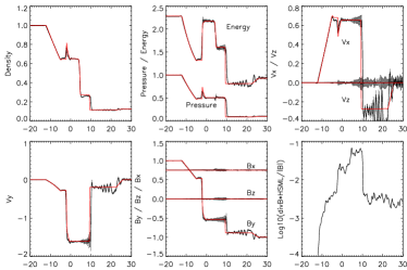
Figure 1: Test 5A at time $t=7$ with the MHD implementation similar to that used in Dolag et al. (1999, 2002), but already including the instability correction due to subtraction of the $\mathrm{div}(\vec{B})$ term in the force equation and in a fully three-dimensional setup. Shown in the first row are the density (left panel), total energy and pressure (middle panel) and the $x$,$z$ component of the velocity field (right panel). The second row shows the $y$-component in the velocity field (left panel), the three components of the magnetic field (middle panel) and the measure of the $\mathrm{div}(\vec{B})$ error, see equation (32), in the right panel. The black lines with error bars show the SPH results, the red lines are the reference results obtained with Athena in a 1D setup.

2.7.4 Artificial magnetic dissipation

Another possibility to regularize the magnetic field was presented by Price & Monaghan (2004a), who suggested including an artificial dissipation for the magnetic field, analogous to the artificial viscosity used in SPH. In Price & Monaghan (2004a) it was suggested that the dissipation terms be constructed based on the magnetic field component perpendicular to the line joining the interacting particles. However, to better suppress the small scale fluctuations within the magnetic field which appear due to numerical effects especially in multi-dimensional tests, Price & Monaghan (2004b) suggested basing the artificial dissipation on the change of the total magnetic field rather than on the perpendicular field components only. We also found this to work significantly better in our test cases and therefore only use the later implementation throughout this paper. Such an artificial dissipation term can be included in the induction equation as

$$\left(\frac{\mathrm{d}\vec{B}_{i}}{\mathrm{d}t}\right)^{(\mathrm{diss})} = \frac{1}{Ha^{2}}\frac{\rho_{i}\alpha_{B}}{2}$$ (26)

$$\sum_{j=1}^{N}\frac{m_{j}v_{ij}^{\mathrm{sig}}}{\hat{\rho}_{ij}^{2}}\left(\vec{B}_{i}-\vec{B}_{j}\right)\frac{\vec{r}_{ij}}{|\vec{r}_{ij}|}\cdot\vec{\nabla}_{i}W_{i}.$$

The parameter $\alpha_{B}$ is used to control the strength of the effect, typical values are suggested to be around $\alpha_{B}\sim 0.5$. Similar to the artificial viscosity, this will create entropy at the rate

$$\left(\frac{\mathrm{d}A_{i}}{\mathrm{d}t}\right)^{(\mathrm{diss})} = -\frac{\gamma-1}{\rho_{i}^{\gamma-1}}\frac{\alpha_{B}}{4\mu_{0}}$$ (27)

$$\sum_{j=1}^{N}\frac{m_{j}v_{ij}^{\mathrm{sig}}}{\hat{\rho}_{ij}^{2}}\left(\vec{B}_{i}-\vec{B}_{j}\right)^{2}\frac{\vec{r}_{ij}}{|\vec{r}_{ij}|}\cdot\vec{\nabla}_{i}\bar{W}_{ij}.$$

The pre-factor $(\gamma-1)/(\rho_{i}^{\gamma-1})$ properly converts the dissipation term to a change in entropy.

This method reduces noise significantly. However, depending on the choice of $\alpha_{B}$, it can also lead to smearing of sharp features. To avoid this outside of strong shocks (e.g. where this is needed), Price & Monaghan (2005) proposed evolving $\alpha_{B}$ for each particle, similar to the handling of the time dependent viscosity as suggested by Morris & Monaghan (1997). Such, evolution of $\alpha_{B}$ for each particle will be followed by integrating

$$\frac{\mathrm{d}\alpha_{B}}{\mathrm{d}t}=-\frac{(\alpha_{B}-\alpha_{B}^{\mathrm{min}})}{\tau}+S,$$ (28)

where the source term $S$ can be chosen as

$$S=S_{0}\,\mathrm{max}\left(\frac{|\vec{\nabla}\times\vec{B}|}{\sqrt{\mu_{0}\rho}},\frac{|\vec{\nabla}\cdot\vec{B}|}{\sqrt{\mu_{0}\rho}}\right)$$ (29)

(see Price & Monaghan, 2005). The time-scale $\tau$ defines how fast the dissipation constant decays. Taking the signal velocity, one can translate this directly into a distance to the shock over which the dissipation constant decays. A useful choice of $\tau$ can be written as

$$\tau=\frac{h_{i}}{C\;v_{\mathrm{sig}}},$$ (30)

where the constant $C$ typically is chosen to be around 0.2, allowing the dissipation constant to decay within a time that corresponds to the shock travelling 5 kernel lengths (see Price & Monaghan, 2004a),

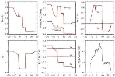
Figure 2: As figure 1, but including the magnetic waves in the signal velocity and turning off the shear viscosity suppression as explained in the code description. The main advantage is a significant reduction in the noise, specifically in the velocity, but also in the magnetic field. Also the $\mathrm{div}(\vec{B})$ errors are reduced by a factor of $\approx 2$.

2.8 Euler potential

A very elegant way to implement the MHD equations in Lagrangian codes is the usage of so called Euler potentials (see Rosswog & Price, 2007, and references therein). Two independent variables $\alpha$ and $\beta$ are constructed to correspond to an implicit gauge for the vector potential. They can be thought of as labels of magnetic field lines and will be advected with the flow. In this formulation, the magnetic field at any time can be represented as

$$\vec{B}=\vec{\nabla}\alpha\times\vec{\nabla}\beta.$$ (31)

In principle, having obtained the magnetic field, one could also use this magnetic field in the equation of motion as before. However, this would mean that the magnetic force is based on the second derivative of a variable. This is usually quite noisy and not recommendable unless regularization schemes are implemented as done by e.g. Rosswog & Price (2007). In addition, due to its form, an implementation based on the Euler potential cannot be easily investigated in 3D test problems with periodic boundary conditions for the resulting magnetic field as can be done for the other implementations. A simple example here is constant magnetic field, which can be represented by a linear function of the Euler potentials.

Therefore we use this simple description only as a check in cosmological simulations, to investigate the influence of $\mathrm{div}(\vec{B})$ driven errors. Applied to cosmological simulations the evolution of the magnetic field predicted when using Euler potentialsis an upper bound on the amplification processes in the absence of any dynamo action. Therefore Euler potentials are a useful tool to check the influence of numerics on the results of cosmological simulations where we have no other means to verify the results.

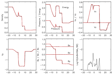
Figure 3: As figure 2, but including the regular smoothing of the magnetic field as a regularization scheme. This SPH-MHD implementation basically reflects the one used in Dolag et al. (2004, 2005). The main advantages are a further, significant reduction in the noise as well as a strong reduction of the $\mathrm{div}(\vec{B})$ errors by a factor of $\approx 10$.

3 Test problems

To test performance of the code and to infer the optimal numerical settings for the regularization schemes, we performed the series of shock-tube problems as presented by Ryu & Jones (1995). In particular test 5A, which is also used in Brio & Wu (1988), was used to show the effects of different numerical treatments. Additionally we performed several 2D test cases including the Fast Rotor test (Tóth, 2000; Londrillo & Del Zanna, 2000; Balsara & Spicer, 1999), a Strong Blast (Londrillo & Del Zanna, 2000; Balsara & Spicer, 1999) and the Orzang-Tang Vortex (Orzang & Tang, 1979; Dai & Woodward, 1994; Picone & Dahlburg, 1991; Londrillo & Del Zanna, 2000). To obtain results under realistic circumstances, we performed all the tests by setting up a fully three-dimensional particle distribution. We also avoid starting from regular grids but used glass-like (White, 1996) initial particle distributions instead. To obtain such a configuration, the particles are originally distributed in an random fashion within the volume and then allowed to relax until they settle in a equilibrium distribution which is quasi force-free and homogeneous in density. This is similar to the distribution of atoms in an amorphous structure like glass. Compared to a distribution of the particles based on a grid, this guarantees that all the kernel averages in the SPH formalism sample the kernel in a uniform way rather than multiple times at the same distances (which furthermore would be fractions of the underlying grid spacing). For all tests we used the same particle masses, independent of the initial density. Therefore, typical initial particle distributions for the shock-tube tests where based on $5^{3}$ particles in low density and $10^{3}$ particles in high density regions within unit volume. Usually, these unit volumes are then replicated 35 times along the $x$-direction each. For some test cases with strong (and therefore fast) shocks, we evolved the simulations longer. In such cases we doubled the simulation setup size in the $x$-direction.

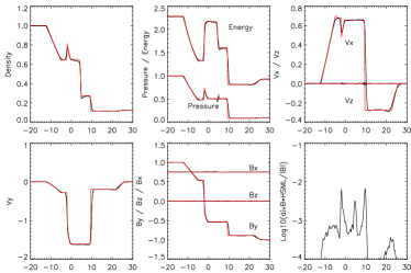
Figure 4: As figure 2, but including artificial magnetic dissipation as a regularization scheme. Similar to the smoothing of the magnetic field, significant reduction in the noise as well as a strong reduction of the $\mathrm{div}(\vec{B})$ errors by a factor of $\approx 10$ is obtained compared to the basic SPH-MHD implementation.

We assume ideal gas (e.g. $\gamma=5/3$) and, as described before, use an equivalent of 64 neighbors for calculating the SPH smoothing length. This ensures that, in the low density regions, the SPH particles get smoothed over a region corresponding to a unit length. The number of resolution elements corresponding to a unit length therefore ranges from 1 to 4, depending whether one associates the smoothed region or the mean inter-particle distance with the effective resolution in SPH. In general, SPH converges somewhat slower compared to grid codes when comparing simulations with the same number of grid cells as SPH particles (see Appendix A for an example).

For the SPH results we usually plot the mean within a 3D slab corresponding to the smoothing length and (as error bars) the RMS over the individual particles within this volume. The reference solution was obtained using Athena (Stone et al., 2008) with typically 10-20 resolution elements per unit length, depending on the individual test. As one criteria of the goodness of the SPH simulation result we use the usual measure for the non-vanishing divergence of the magnetic field,

$$E_{\nabla\vec{B}}=\mathrm{div}(\vec{B})\frac{h}{|\vec{B}|}.$$ (32)

3.1 Shock tube 5A

The most commonly used MHD shock-tube test is the one used by Brio & Wu (1988), e.g. test 5A in Ryu & Jones (1995). The reason for this is that it involves a shock and a rarefraction moving together. Therefore it allows simultaneous testing of the code in different regimes.

Figure 1 shows the result for a code implementation similar to the first implementation used to study galaxy clusters (e.g. see Dolag et al., 1999, 2002). In addition, the instability correction due to subtraction of the $\mathrm{div}(\vec{B})$ term was used in the force equation. Various hydro-dynamical variables at the final time (e.g. $t=7$ in this case) are shown. The black lines with error bars show the SPH-MHD result, the red lines are the reference result obtained with Athena in a 1D setup. Shown are (from upper left to the bottom right panel) the density, total energy and pressure, the $x$- and $z$-component of the velocity field, the $y$-component in the velocity field, the three components of the magnetic field and the measure of the $\mathrm{div}(\vec{B})$ error, obtained from equation (32). Here we also switched back to the conventional formulation of the artificial viscosity as described by e.g. Monaghan (1992), rather than that based on signal velocity as used in GADGET-2. Although the SPH-MHD results in general follow the solution obtained with Athena, there is a large scatter in the individual particle values within the 3D volume elements, as well as some instability, especially in the low-density part. But note that although the mean values for the internal energy, as well as the velocity or magnetic field, can locally show some systematic deviations from the ideal solution, the total energy shows much better, nearly unbiased, behaviour. This demonstrates the conservative nature of the symmetric formulations in SPH-MHD.

Noticeable reduction of noise is obtained when using the signal-velocity based artificial viscosity and including the magnetic waves in the calculation of the signal velocity. Therefore, the magnetic waves are directly captured for the time step calculation and in the artificial viscosity, needed to capture shocks. Also switching off the shear viscosity suppression again leads to significant reduction in scatter. This can be seen in figure 2, where the noise in the velocity as well as in the magnetic field components is significantly reduced. Values of $\mathrm{div}(\vec{B})$ are also reduced (by a factor of $\approx 2$) compared to before. In general, the SPH-MHD implementation gains from the new formulation of SPH, including the $\frac{\mathrm{d}W}{\mathrm{d}h}$ terms and the new way to determine the SPH smoothing length, both contributing to a reduction of noise (and $\mathrm{div}(\vec{B})$) in the general treatment of hydro-dynamics. We will refer to this implementation of SPH-MHD as basic SPH-MHD further on in this paper.

3.2 The effect of regularization

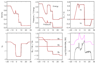
Figure 5: As figure 2, but including time dependent artificial magnetic dissipation as a regularization scheme. No significance improvement is obtained. Note that here in the lower right panel the artificial dissipation constant ($\alpha_{B}$) is shown. The effect of suppressing the dissipation is clearly visible, and the maximum value is only reached in peaks associated with the region of strong shocks. However the improvement in the smearing of sharp features is not very significant.

As described in section (2.7), there are several suggestions for regularization of the magnetic field. Here we will show results obtained by two regularization methods, namely smoothing the magnetic field in regular intervals and including an artificial dissipation.

TEST Nr.	Left				Right
	$\rho$	${V}$	${B}$	$P$	$\rho$	${V}$	${B}$	$P$
— 1A —	1.00	$[10.0,0.0,0.0]$	$[5.0,5.0,0.0]/(4\pi)^{2}$	20.0	1.000	$[-10.0,0.0,0.0]$	$[5.0,5.0,0.0]/(4\pi)^{2}$	1.00
— 1B —	1.00	$[0.0,0.0,0.0]$	$[3.0,5.0,0.0]/(4\pi)^{2}$	1.0	0.100	$[0.0,0.0,0.0]$	$[3.0,2.0,0.0]/(4\pi)^{2}$	10.0
— 2A —	1.08	$[1.2,0.01,0.5]$	$[2.0,3.6,2.0]/(4\pi)^{2}$	0.95	1.000	$[0.0,0.0,0.0]$	$[2.0,4.0,2.0]/(4\pi)^{2}$	1.00
— 2B —	1.00	$[0.0,0.0,0.0]$	$[3.0,6.0,0.0]/(4\pi)^{2}$	1.0	0.100	$[0.0,2.0,1.0]$	$[3.0,1.0,0.0]/(4\pi)^{2}$	10.0
— 3A —	1.00	$[50.0,0.0,0.0]$	$-[0.0,1.0,2.0]/(4\pi)^{2}$	0.4	0.100	$[0.0,0.0,0.0]$	$[0.0,1.0,2.0]/(4\pi)^{2}$	0.20
— 3B —	0.10	$[-1.0,0.0,0.0]$	$[0.0,1.0,0.0]$	1.0	1.000	$[1.0,0.0,0.0]$	$[0.0,1.0,0.0]$	1.00
— 4A —	1.00	$[0.00,0.0,0.0]$	$[1.0,1.0,0.0]$	1.0	0.200	$[0.0,0.0,0.0]$	$[1.0,0.0,0.0]$	0.10
— 4B —	0.40	$[-0.669,0.986,0.0]$	$[1.3,0.0025293,0.0]$	0.5247	1.000	$[0.0,0.0,0.0]$	$[1.3,1.0,0.0]$	1.00
— 4C —	0.65	$[0.667,-0.257,0.0]$	$[0.75,0.55,0.0]$	0.50	1.000	$[0.4,-0.94,0.0]$	$[0.75,0.00001,0.0]$	0.75
— 4D —	1.00	$[0.0,0.0,0.0]$	$[7.0,0.001,0.0]$	1.0	0.300	$[0.0,0.0,0.0]$	$[7.0,1.0,0.0]$	0.20
— Brio Wu —	1.00	$[0.0,0.0,0.0]$	$[0.75,1.0,0.0]$	1.0	0.125	$[0.0,0.0,0.0]$	$[0.75,-1.0,0.0]$	0.10

Table 1: Summary table with the initial conditions of the left and right side of the shock tubes.

For the first method, the magnetic field is smoothed using the same kernel as used for the normal SPH calculations. In this case, there are two numerical parameters one can choose. One is $q$ in equation (25), which quantifies the weight with which the smoothed component enters into the updated magnetic field. We always use $q=1$ here, which means that we completely replace the magnetic field by the smoothed value. The second is $T_{\mathrm{BS}}$, which is the time interval at which the smoothing is done. Here we use a value corresponding to a smoothing every 30^th global time step. This correspond to the SPH-MHD implementation used to study the magnetic field in clusters and large scale structure within the local universe, see Dolag et al. (2004, 2005). Figure 3 shows the result for the same shock-tube test as before. Clearly, the noise in the individual quantities is strongly reduced. Also the error in $\mathrm{div}(\vec{B})$ is reduced by more than one order of magnitude. Note that the error bars for the SPH-MHD implementation are of the size of the line width or smaller in most of the cases and therefore no longer clearly visible. However, one can notice some small effect of smearing sharp features. Additinalally, some states – like the region with the negative $x$-component of the velocity behind the the fast rarefaction wave propagating to the right – converge to values which have small but systematic deviations from the exact solution.

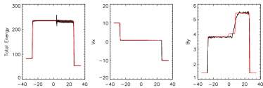
(a) Test 1A

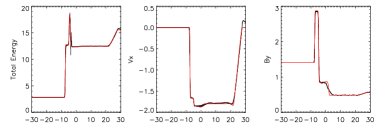
(b) Test 1B

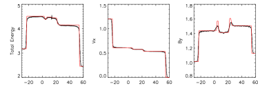
(c) Test 2A

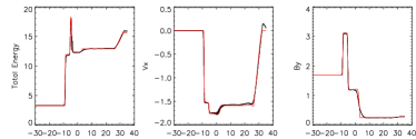
(d) Test 2B

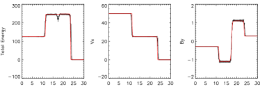
(e) Test 3A

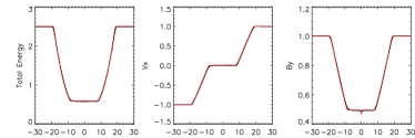
(f) Test 3B

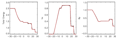
(g) Test 4A

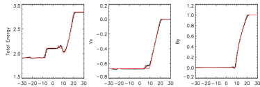
(h) Test 4B

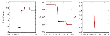
(i) Test 4C

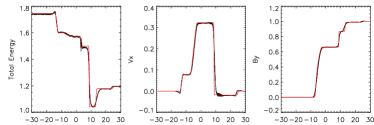
(j) Test 4D

Figure 6: Representative plots of the additional 10 shock-tube tests from Ryu & Jones (1995). Shown for each test are the total energy (left panels), the velocity along the $x$-direction (middle panels) and the magnetic field along the $y$-direction (right panels).

In the second method, the magnetic field can be dissipated in the same way as artificial dissipation works in the hydrodynamics. Here the numerical parameter one has to chose is the strength of this artificial, magnetic dissipation $\alpha_{B}$ in equation (26) and (27). Figure 4 shows the result for the same shock-tube test as before using $\alpha_{B}=0.1$. Similar to the first regularization method presented, the noise in the individual quantities is strongly reduced and also the error in $\mathrm{div}(\vec{B})$ is reduced by one order of magnitude. Again, the error bars are smaller than the line width nearly everywhere. Also, some small effects of smearing sharp features are visible as well as some small but systematic deviations from the exact solution. In general, this method works slightly better than the smoothing of the magnetic field, but the differences are generally small.

One idea to reduce the unwanted side effects of such regularization schemes was presented in Price & Monaghan (2005) and is based on a modification of the artificial, magnetic dissipation constant $\alpha_{B}$. Whereby every particle evolves its own numerical constant, so that this value can decay where it is not needed and therefore the effects of the artificial dissipation are suppressed here. Figure 5 shows the same test as before, but this time where $\alpha_{B}$ evolves for each particle, as shown in the lower right panel. Clearly, the values are strongly reduced outside the regions associated with sharp features (e.g. shocks), but the effect of smearing sharp features and the small offset of some states are not significantly reduced. This is because in the region in which these side effects originate, the dissipation is still working with its maximum numerical value. On the other hand, due to the suppression of the artificial magnetic dissipation constant outside the shock region, the regularization after the shock passes is nearly switched off. Therefore it is not as efficient as before in the post shock region, visible as increase in the $\mathrm{div}(\vec{B})$ error compare to the run with a constant, artificial magnetic dissipation.

3.3 Shock tube problems

As can be seen in figures 3 and 4, the side effects of smoothing features by the different regularization methods depend on the details of the underlying structure of the shock-tube test. Even more interesting, the states where one can see small deviations from the ideal solution are different for the two different regularization methods. Therefore we performed the full set of different shock-tube tests as presented in Ryu & Jones (1995) to test the overall performance of the different implementations under different circumstances. The four test families deal with different complexities of velocity and magnetic field structures, leading to different kinds of waves propagating. A summary of the results of these tests can be found in figure 6. Plotted are the total energy (left panels), the velocity along the $x$-direction (middle panels) and the magnetic field along the $y$-direction (right panels). The red lines reflects the ideal solution obtained with Athena, the black lines with error bars mark the results from the SPH-MHD implementation using the magnetic field smoothing every 30th main time step. Note that the error bars in most cases are smaller than the line width. The initial setups for the shock-tube tests can be found in table 1, which lists the state vector of the left and right states for the different shock tube tests.

The first family of tests (1A/1B) has no structure in the tangential direction of the propagating shocks in magnetic field and velocity, e.g. $B_{z}=v_{z}=0$. As we expect, in the 1A test, the strong shock (large jump in $v_{x}$) leads to some visible noise in the magnetic field component $B_{y}$, also translating into significant noise in the total energy. The regularization method here suppresses the formation of the intermediate state in $B_{y}$ in the SPH-MHD implementation, as can be seen in figure 6(a). The second case, the 1B test, the weak shock is captured well. Again in some regions some smearing of sharp features due to the regularization method is clearly visible.

The second class of shocks (2A/2B) involve three dimensional velocity structures, where the plane of the magnetic field rotates. All features (e.g. fast/slow shocks, rotational discontinuity and fast/slow rarefaction wave, for details see Ryu & Jones (1995)), are well captured, see figure 6(c) and 6(d). Some of the features are clearly smoothed by the regularization method.

The third class of tests (3A/3B) shows handling of magnetosonic structures. The first has a pair of magnetosonic shocks with zero parallel field and the second are magnetosonic rarefractions. Although there is slightly more noise present, all states are captured extremely well, except the numerical feature left at the position dividing the two states initially, see figure 6(e) and 6(f).

The fourth test family (4A/4B/4C/4D) deals with the so-called switch-on and switch-off structures. The tangential magnetic field turns on in the region behind switch-on fast shocks and switch-on slow rarefractions. Conversely, in the switch-off slow shocks and switch-off fast rarefractions the tangential magnetic field turns off. Again, all structures are captured well with the exception of one feature in figure 6(h) as well and maybe 6(j) too, where clearly the regularization leads to the washing out of a state. Otherwise the regularization leads to smoothing of some structures similar to the tests presented before.

In general, figure 6 demonstrates that all these different situations have to be included when trying to measure the performance and quality of different implementations of regularization methods.

3.4 Finding optimal numerical parameters

To optimize, we performed all these 11 shock-tube tests with various different settings for the parameters in the regularization methods and evaluated the quality of the result obtained with the SPH-MHD implementation. To measure this, we used two estimators. First, we have chosen the mean of all $\mathrm{div}(\vec{B})$ errors within the simulation region shown in the plots, as defined by

$$\Delta_{\mathrm{div}(\vec{B})}=\left<\mathrm{div}(\vec{B})\frac{h}{|\vec{B}|}\right>_{x}.$$ (33)

Second, we measured the discrepancy of the SPH-MHD result for the magnetic field relative to the results obtain by Athena. Therefore we calculate first

$$\delta_{B^{i}}(x)=\frac{\left(\vec{B}_{\mathrm{SPH}}^{i}(x)-\vec{B}_{\mathrm{Athena}}^{i}(x)\right)^{2}}{\mathrm{RMS}_{B^{i}}^{2}(x)}$$ (34)

for each component $i$ of the magnetic field $\vec{B}$ within each 3D slab corresponding to the smoothing length. The RMS of $B^{i}$ reflects the noise of $B_{i}$ within the chosen slab. We then calculate

$$\hat{\Delta}_{B^{i}}=\left(\sum_{x}\delta_{B^{i}}(x)\right)\left(\sum_{x}\mathrm{RMS}_{B^{i}}^{2}(x)\right),$$ (35)

for each component of the magnetic field. This includes both contributions, the deviation of the SPH-MHD from the ideal solution as well as the noise within each 3D slab of the SPH-MHD implementation. To judge the improvement of the regulatization methods we sum up all three components and further relate this measurement to the value obtained with the basic SPH-MHD implementation, e.g.

$$\Delta_{B}=\frac{\sum_{i}\hat{\Delta}_{B^{i}}}{\sum_{i}\hat{\Delta}_{B^{i}}^{\mathrm{std}}}-1.$$ (36)

We will use these two error estimators, $\Delta_{\mathrm{div}(\vec{B})}$ and $\Delta_{B}$, to measure the quality of the individual SPH-MHD implementations.

3.4.1 Regularization by smoothing the magnetic field

Choosing the time interval between smoothing the magnetic field is a compromise between reducing the noise in the magnetic field components, as well as $\mathrm{div}(\vec{B})$) (by smoothing more often) and preventing sharp features from being smeared out. The left two panels of Figure 7 show a summary of the results of the individual shock-tube test computed with different smoothing intervals. As expected, when using shorter smoothing intervals the error in $\mathrm{div}(\vec{B})$ reduces. For the quality measure of the SPH-MHD implementation the situation changes. Short smoothing intervals generally increase the discrepancy, many of them even to larger values than the basic SPH-MHD run. Specifically 4B and 4C show strong deviations due to smearing of sharp features. Note that the non monotonic behavior shown in some tests usually relates to some residual resonances between the magnetic waves and the smoothing intervals in the noise. Some tests show a minimum in the differences at smoothing intervals around 20. The test 3A seems to prefer even shorter smoothing intervals. In general is not clear how an optimal decision between such quality measure and the reduction in $\mathrm{div}(\vec{B})$ can be reached, given the different nature and amplitude of the two measures. However, ignoring 4B which strongly suffers from smearing sharp features when smoothing the magnetic field, a good compromise seems to be for values around 20-30, where pro and con in the quality measure are small and compensating within the different tests but $\mathrm{div}(\vec{B})$ is still drastically reduced in all tests. We will refer to this as the Bsmooth SPH-MHD implementation in the rest of the paper.

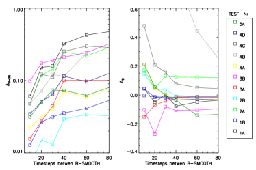
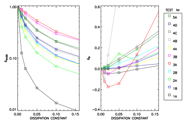
Figure 7: Shown in the two left panels are the mean error in divergence (first panel on the left) and the measure of the quality (second panel from left) as defined in equation (36) obtained by the SPH-MHD implementation for different values of the smoothing interval. The different lines are for the 11 different shock-tube tests as indicated by the labels. The two right panels show the same quantities but for different values of the artificial magnetic dissipation constant $\alpha_{B}$.

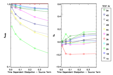
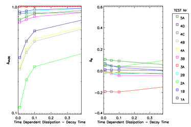
Figure 8: Similar to figure 7 but for different values of the source term $S_{0}$ (left panels) and the decay term $C$ (right panel) of the time dependent, artificial magnetic dissipation.

3.4.2 Artificial dissipation

As before, choosing the value for the artificial magnetic dissipation constant $\alpha_{B}$ is a compromise between reducing the noise in the magnetic field components (as well as reducing $\mathrm{div}(\vec{B})$) and preventing sharp features from smearing out due to the effect of the dissipation. The right two panels of Figure 7 show a summary of the results of the individual shock-tube tests computed with different values for the artificial magnetic dissipation. As expected, using larger values reduces the error in $\mathrm{div}(\vec{B})$ significantly. Similar to before, using larger values also generally results in an increase of the discrepancy between the SPH MHD implementation and the true solution, again usually to even larger values than in the basic SPH-MHD run. As before, especially the shock-tube test 4B and 4C show strong deviations due to smearing of sharp features. Note that here less non-monotonic behavior is visible (except for test 4B). The main reason is that dissipation is a continuous process, so resonances between dissipation and the magnetic waves cannot be very pronounced. As before, it is difficult to infer the best choice of parameter for all the tests. Again, once ignoring 4B, a compromise for choosing $\alpha_{B}$ seems to be between 0.02 and 0.1. Choosing $\alpha_{B}$ close to the upper value of 0.1 might lead to a significant reduction in $\mathrm{div}(\vec{B})$ without to strong signature from smearing out sharp features. We will refer to this as the dissipation SPH-MHD implementation in the rest of the paper.

3.4.3 Time dependent artificial dissipation

One idea to reduce the effect of the artificial dissipation is to make the artificial magnetic dissipation constant $\alpha_{B}$ time dependent. The idea here is that, if the evolution of $\alpha_{B}$ is properly controlled, dissipation will happen only at the places where it is needed and it will be suppressed in all other parts of the simulation volume. The evolution of $\alpha_{B}$ is controlled by the two parameters $S_{0}$ (source term) and $C$ (decay term) where we have chosen $\alpha_{B}^{\mathrm{min}}$ and $\alpha_{B}^{\mathrm{max}}$ as 0.01 and 0.5 respectively. Figure 8 shows the result for varying these two parameters. As before, generally, the larger the dissipation is (e.g. large source term or small decay time) the smaller the noise and the error in $\mathrm{div}(\vec{B})$ becomes. However, as soon as these parameters have values which drive $\alpha_{B}$ in the shocks to the maximum allowed value, there is marginally no gain in quality, although the values for $\alpha_{B}$ outside the shocks can still be quite small. Therefore, the time dependent method does not improve the results significantly, as the regions in which the artificial dissipation constant is suppressed do not significantly contribute to the smearing of sharp features.

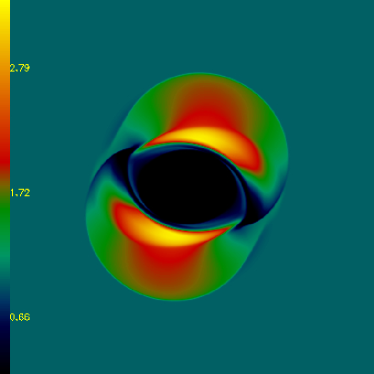
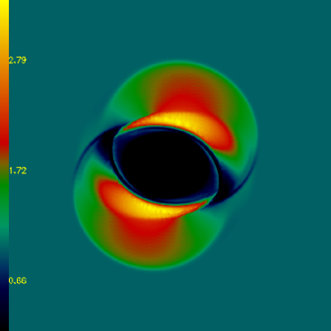
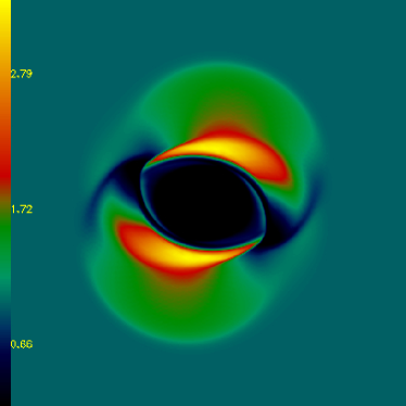
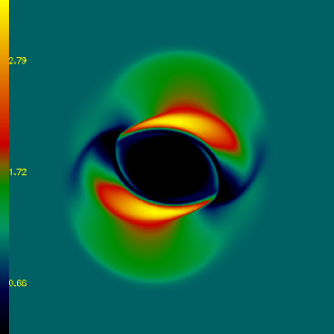
Figure 9: The magnetic pressure ($B^{2}/2$) in the Fast Rotor test at $t=0.1$. The ATHENA solution of the test problem is shown in the upper left panel. The upper right panel shows the results obtained with the basic SPH-MHD implementation. The lower left and right panels shows the result obtained with the Bsmooth SPH-MHD and the dissipation SPH-MHD implementation respectively. All the main features are well reproduced in the GADGET runs. The shape, positions and amplitudes correspond quite well, although the GADGET runs appear slightly more smoothed, depending on the regularization scheme used (see also Figure 10).

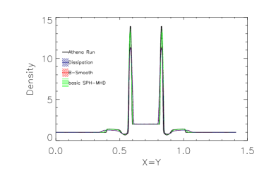
Figure 10: Diagonal ($x=y$) cut through the Fast Rotor at $t=0.1$ showing the density. In black result obtained with ATHENA. The pink line with the red error bars show the GADGET solution using the basic SPH-MHD implementation. Also here the red error bars reflect the dispersion of the values among individual particles within a slab corresponding to the local smoothing length. In general, the SPH-MHD result shows an excellent agreement in all the features (peaks, valleys and edges), however there is a visible over-smoothing at the outer edges in the GADGET result.

3.5 Multi dimensional Tests - Planar Tests

Besides the one dimensional shock tube test described in the previous section, two dimensional (e.g. planar) test problems are a good test-bed to check code performance. Such higher dimensional tests include additional interaction between the evolving components with non-trivial solution. These can be quite complex (with several classes of waves propagating in several directions) such as the Orszang-Tang Vortex or simple (but with strong MHD discontinuities) such as Strong Blast or Fast Rotor.

3.5.1 Fast Rotor

This test problem was introduced by Balsara & Spicer (1999), to study star formation scenarios, in particular the strong torsional Alfvén waves, and is also commonly used to validate MHD implementations (for example see Tóth, 2000; Londrillo & Del Zanna, 2000; Price & Monaghan, 2005; Børve et al., 2006). The test consists of a fast rotating dense disk embedded in a low density, static and uniform media, with a initial constant magnetic field along the x-direction (e.g. $B_{x}=2.5\pi^{-1/2}$). In the initial conditions, the disk with radius $r=0.1$, density $\rho=10$ and pressure $P=1$ is spinning with an angular velocity $\omega=20$. It is embedded in a uniform background with $\rho=P=1$. Again we setup the initial conditions by distributing the particles on a glass like distribution in 3D, using $700\times 700\times 5$ particles and periodic boundaries in all directions for the background particles. The disk is created by removing all particles which fall inside the radius of the disk and replacing this space with a denser representation of particles of the same mass. As an ideal solution to compare with, we again used the result of a simple, two dimensional ATHENA run with $400\times 400$ cells. A visual impression of the results can be obtained from the maps presented in figure 9.

Figure 10 presents another quantitative comparison. Shown is a diagonal cut through the Fast Rotor at $t=0.1$ showing the density. The different lines show the result obtained with ATHENA (black line) and for the three different SPH-MHD implementations in GADGET (colored lines). The very small, red error bars reflect the RMS of the values held by the individual particles within the 3D slab through the three dimensional simulations corresponding to the local smoothing length. The results show remarkable agreement between the simulations and also compare well with results quoted in the literature (e.g. Londrillo & Del Zanna, 2000). Here the smoothing of sharp features in the two implementations with regularization is quite clear visible and leads to a less good match than the basic SPH-MHD implementation.

Note that although we perform our calculations in three dimensions and without a regularization scheme, the implementation produce a result, which has the same quality as other schemes in two dimensions with regularization (e.g. Price & Monaghan, 2005; Børve et al., 2006).

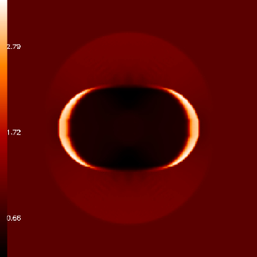
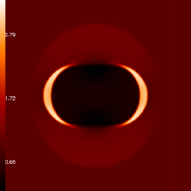
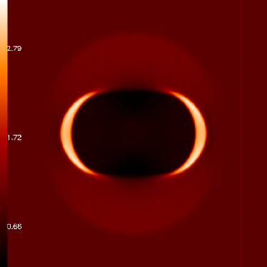
Figure 11: Shown is the resulting density distribution for the Strong Blast test at $t=0.02$. The upper left panel shows the result obtained with ATHENA, whereas the upper right panel shows the that from the basic SPH-MHD implementation. The lower left and right panels shows the results obtained with the Bsmooth SPH-MHD and the dissipation SPH-MHD implementation respectively. There are no visible difference between the results (see also figure 12), indicating that all SPH-MHD implementations are capable to handle such test situation.

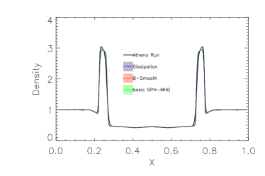
Figure 12: Horizontal cut through the Strong Blast test ($x=[0.0;1.0],y=0.5$) showing the density. The black line is from the ATHENA simulation, the pink line with the red error bars (see figure 10) reflects the GADGET result. The overall behavior is excellent, with only very small differences between the two solutions.

3.5.2 Strong Blast

The Strong Blast test consists of the explosion of a circular hot gas in a static magnetized medium and is also regularly used for MHD code validation (see for example Londrillo & Del Zanna, 2000; Balsara & Spicer, 1999). The initial conditions consist of a constant density $\rho=1$ where a hot disk of radius $r_{0}=0.125$ is embedded, which is a hundred times over-pressured, e.g the pressure in the disk is set to $P_{d}=100$ whereas the pressure outside the disk is set to $P_{o}=1$. In addition there is initially an overall homogeneous magnetic field in the $x$-direction, with a strength of $B_{x}=10$. The system is evolved until time $t=0.02$ and an outgoing shock wave is visible which, due to the presence of the magnetic field, is no longer spherical but propagates preferentially along the field lines. Figure 11 shows the density at the final time, comparing the ATHENA results with the results from the three different SPH-MHD implementations in GADGET. Although the setup is a strong blast wave, there is no visible difference of the SPH-MHD implementation with the ATHENA results. This is quantitatively confirmed in figure 12 which shows a horizontal cut (at $y=0.5$) of the density through the Strong Blast test, comparing the ATHENA (black line) with the GADGET (colored lines with error bars) results. Besides very small variations there is no significant difference between the two results and all features are well reproduced by the SPH-MHD implementation. Note that the error bars of the GADGET results again are almost in all cases smaller than the shown line width.

3.5.3 Orszang-Tang Vortex

This planar test problem, introduced by Orzang & Tang (1979), is well known to study the interaction between several classes of shock waves (at different velocities) and the transition to MHD turbulence. Also, this test is commonly used to validate MHD implementations (for example see Dai & Woodward, 1994; Picone & Dahlburg, 1991; Londrillo & Del Zanna, 2000; Price & Monaghan, 2005; Børve et al., 2006). The initial conditions for an ideal gas with $\gamma=5/3$ are constructed within a unit-length domain (e.g. $x=[0,1],y=[0,1]$) with periodic boundary conditions. The velocity field is defined by $v_{x}=-\sin(2\pi y)$ and $v_{y}=\sin(2\pi x)$. The initial magnetic field is set to be $B_{x}=B_{0}v_{x}$ and $B_{y}=B_{0}sin(4\pi x)$. The initial density is $\rho=\gamma P$ and the pressure is set to $P=\gamma B_{0}^{2}$. This system is evolved until $t=0.5$. Figure 13 shows the final result for the magnetic pressure for the ATHENA run and the three different SPH-MHD implementations in GADGET. Visually the results are quite comparable, however the GADGET results look slightly more smeared, which is the imprint of the underlying SPH and regularization methods. This impression is confirmed in figure 14, which shows two cuts ($y=0.3125$ and $y=0.4277$) through the two simulations. Again, the black line shows the ATHENA result, the colored lines with the error bars are showing the GADGET results. In general there is a reasonable agreement, however the SPH-MHD results clearly show smoothing of features. The adaptive nature of the SPH-MHD implementation should allow the central density peak to be resolved whereas in ATHENA is can only be resolved by increasing the number of grid cells. Never-the-less the SPH-MHD implementation seems to converge slower when increasing the resolution (see Appendix).

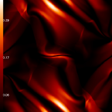
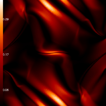
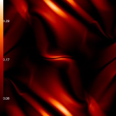
Figure 13: The magnetic pressure $B^{2}/2$ distribution in the Orszang-Tang Vortex at $t=0.5$. The upper left panel shows the result obtained with ATHENA, while the upper right panel shows those from the basic SPH-MHD implementation. The lower left and right panels shows the results obtained with the Bsmooth SPH-MHD and the dissipation SPH-MHD implementations respectively. Some of the sharp features are more smoothed in the GADGET runs, depending on the choice of regularization scheme, but overall the results compare very well (see also figure 14)

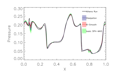
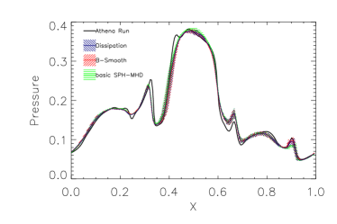
Figure 14: Two $t=0.5$ cuts throught the pressure in the Orszang-Tang Vortex at $y=0.3125$ and at $y=0.4277$ (left and right panels, respectively). As before, the black line reflect the results obtained with ATHENA and the pink line with the red error bars is obtained with the basic SPH-MHD implementation in GADGET. The cuts are choosen for comparison with results from the literature, e.g. Børve et al. (2006).

3.6 General performance of SPH-MHD

In summary, as shown in the previous sections, an MHD implementation in SPH is able to reliable reproduce the results of standard, one and two dimensional MHD test problems. We want to stress the point that all tests for the SPH-MHD implementation where performed in a fully three dimensional setup to test the code under realistic circumstances. Regularization schemes in general are able to further suppress the numerical driven growth of $\mathrm{div}(\vec{B})$. Although some optimal numerical values for the regularization schemes can be inferred when comparing a suit of different shock tube tests, such regularization schemes always introduce small dissipative effects, which lead to a slight smearing of sharp features. This has to be kept in mind when applying the different SPH-MHD implementations to cosmological applications.

4 Cosmological Application

The cluster used in this work is part of a galaxy cluster sample (Dolag et al., 2008) extracted from a re-simulation of a Lagrangian region selected from a cosmological, lower resolution DM-only simulation (Yoshida et al., 2001). This parent simulation has a box–size of $684$ Mpc, and assumed a flat $\Lambda$CDM cosmology with $\Omega_{m}=0.3$ for the matter density parameter, $H_{0}=70$ for the Hubble constant, $f_{bar}=0.13$ for the baryon fraction and $\sigma_{8}=0.9$ for the normalization of the power spectrum. The cluster has a final mass of $1.5\times 10^{14}M_{\odot}$ and was re-simulated at 3 different particle masses for the high resolution region. Using the “Zoomed Initial Conditions” (ZIC) technique (Katz & White, 1993; Tormen et al., 1997), these regions were re-simulated with higher mass and force resolution by populating their Lagrangian volumes with a larger number of particles, while appropriately adding additional high–frequency modes drawn from the same power spectrum. To optimize the setup of the initial conditions, the high resolution region was sampled with a $16^{3}$ grid, where only sub-cells are re-sampled at high resolution to allow for quasi abritary shapes of the high resolution region. The exact shape of each high–resolution region was iterated by repeatedly running dark-matter only simulations, until the targeted objects are free of any lower–resolution boundary particle out to 3-5 virial radii. The initial particle distributions, before adding any Zeldovich displacement, were taken from a relaxed glass configuration (White, 1996). The three resolutions used correspond to a mass of the dark matter particles of $1.6\times 10^{9}M_{\odot}$, $2.5\times 10^{8}M_{\odot}$ and $1.6\times 10^{8}M_{\odot}$ for the 1x, 6x and 10x simulation. The gravitational softening corresponds to $7$, $3.9$ and $3.2$ kpc respectively. For simplicity we assumed an initially homogeneous magnetic field of $10^{-11}$ G co-moving as also used in previous work (Dolag et al., 1999, 2002). Furthermore we applied the regularization by smoothing the magnetic field in the same way as we did in previous work (Dolag et al., 2004, 2005) but also tested the effects of regularization by artificial dissipation for varying values of $\alpha_{B}$.

Figure 15 shows a zoom-in from the full cosmological box down to the cluster. The structures in the outer parts get less pronounced due to the decrease in resolution, which is designed to capture only the very largest scales of the simulation volume. Each panel shows (in clockwise order) a zoom-in by a factor of ten. Finally the elongated box in the lower left panel marks the size of the observational frame shown on the left. For comparison we produced a synthetic Faraday Rotation map from the simulation and clipped it to the shape of the actual observations to give an indication of the structures resolved by such simulations. We used the same linear colorscale for both the observed and the simulated RM map, using the highest resoluton simulation (10x). Note that we added a constant, galactic foreground signal to the simulated RM map to account for the non zero mean in the observed RM map. The dynamical range of the simulation spans more than five orders of magnitudes in spatial dimension, and the size of the underlying box is 6 and 5 times larger than the AMR simulations presented in Dubois & Teyssier (2008) and Brüggen et al. (2005), respectively. Still the resolution of the underlying dark matter distribution is, respectively, 2 and 5 times better than these AMR simulations and the cluster is resolved with more than one million dark matter particles within the virial radius at the 10x resolution. To perform the simulation, the 10x resolution run needed $\approx 730$ CPUh on an AMD Opteron cluster. This again is demonstrating the advantages of the underlying SPH scheme in making large, cosmological zoomed simulations possible.

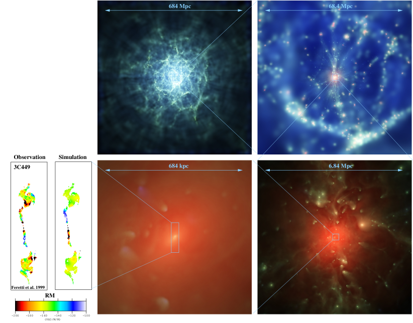
Figure 15: Zoom into the cluster simulated within the cosmological box. Clockwise, each panel displays a factor 10 increase in imaging magnification, starting from the full box (684 Mpc) down to the cluster center (680 kpc). On the very large scale, the density of the dark matter particles are shown, whereas in the high resolution region the temperature of the gas is rendered to emphasize the presence and dynamics of the substructure. The last zoom extracts a region of the same size of an observed radio jet (3C449) with measured rotation measure (Feretti et al., 1999). Both, the simulated and the observed map are displayed using a linear color-scale based on the minimum and maximum values in the maps. The synthetic RM map is clipped to the shape of the observations. Clearly, the simulations are still lacking in resolution, however they do come quite close.

To obtain a more quantitative comparison we calculated the projected structure function $S^{(1)}(d)$ from both the observed and synthetic Faraday Rotation maps.

$$S^{(1)}(\Delta x,\Delta y) =\left<\left|RM(x,y)-RM(x+\Delta x,y+\Delta y)\right|\right>,$$ (37)

with $\Delta x$ and $\Delta y$ being the offsets from a pixel at position $(x,y)$. The resulting matrix is then averaged in radial bins $d=\sqrt{\Delta x^{2}+\Delta y^{2}}$ to obtain the structure function. Figure 16 shows a comparison of the obtained structure function from the observations (black line) and the simulations. For each simulated cluster we calculated the synthetic rotation measure maps, clipped accordingly to the shape of the observed map. To obtain different realizations of the same simulation we produced nine different maps where we shifted the clipped region by $\pm 20$ kpc in both spacial directions within the original, cluster centered maps. The thick lines mark the mean structure function over these maps, whereas the thin lines show the RMS scatter between the different maps. It is clear that, due to the additional resolved turbulent velocity field, when increasing the resolution the same initial seed fields are amplified more. For our 10x simulation the chosen magnetic seed field gets amplified to the observed level in our example cluster. Although increasing the resolution resolve smaller scales in the RM maps, the slope of the structure function at small separations, even the 10x resolution simulation, gets not as steep as the observed one. This confirms the visual impression from the lower left panel in Figure 15 which also indicates more structure at small scales in the observed than the simulated RM map. Pushing the mass resolution by one more order of magnitude would probably result in a spacial resolution which should be sufficient to reproduce the observed small scale structure in the RM maps, however in such a case we would expect to have to start from even smaller seed fields to avoid overestimating the amplitude of the Rotation Measure in the simulations. Such a study lies outside of the scope of this paper, as it ultimately would lead to questions of the role of magnetic dissipation and viscosity within the real intra cluster medium.

In figure 17, the radial magnetic field profiles are shown for the three resolutions comparing the results obtained with the normal configuration for cosmological simulations with results where we just used the Euler Potential to follow the evolution of the magnetic field ignoring back reactions. As already noted in earlier work (Dolag et al., 2002), the left panel shows the dependence of the amplification of magnetic fields with resolution. In addition, the solution obtained with the Euler Potential agrees nicely with the Bsmooth SPH-MHD runs in the outer part of the profiles. It is important to note that the increase in amplification of the magnetic field with increasing resolution when using the Euler Potential clearly demonstrates that this effect originates from resolving more velocity structure, especially driven by the increased amount of substructure in the underlying dark matter representation. Thus the result reflects the increased complexity of the structures in the density and velocity fields, once the resolution of a cosmological simulation is increased. The Euler Potential implementation provides an unique possibility to study these effects as they reflect the result of integrating the wind–up of the complex flows within galaxy clusters, revealing information which can not easily be obtained in Eulerian schemes. In the central parts, the Bsmooth SPH-MHD simulation falls below the solution obtained using the Euler Potential. This is easy to understand, because the Euler Potential are free from any numerical magnetic dissipation. Additionally the magnetic field is strongest in the cluster core and therefore, including the magnetic force in the normal runs will lead to a suppression of the amplification. In general the comparison of the two methods demonstrate that the amplification of the magnetic field in the bsmooth SPH-MHD implementation is not significantly influenced by the non-zero $\mathrm{div}(\vec{B})$. In addition, although the absolute value of the amplification is not converged with resolution, the shape of the predicted magnetic field profile appears to be converged. This is shown in the right panel of figure 17, where the profiles are normalized artificially at large radii to demonstrate the self similar shapes. Note that this convergence, as usual for all hydro-dynamical quantities, is only reached at radii significant larger than the size of the gravitational softening, indicated as dashed lines for the lowest (e.g. 1x), medium (e.g. 6x) and highest (e.g. 10x) resolution runs. In both panels of Figure 17 we also show the results from a cluster simulation using RAMSES, taken from Dubois & Teyssier (2008), and FLASH, taken from Brüggen et al. (2005). This comparison is over-simplistic, as results are based on simulations of different objects and can only be compared with some care. Nevertheless, the shape of the radial profiles obtained with RAMSES indicate slightly more dissipative effects compared to our Bsmooth SPH-MHD implementation, whereas the steeper profile obtained with FLASH resembles our results using the Euler Potential implementation.

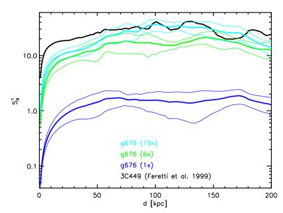
Figure 16: Shown is the structure function averaged in radial bins (for details see text) calculated from the observed (black line) and from the synthetic Faraday Rotation maps (colored lines). The different colors correspond to different resolutions (1x, 6x and 10x). The thick lines correspond to the mean calculated over 9 realizations of the maps, whereas the thin lines mark the RMS scatter between the different maps (see text for details).

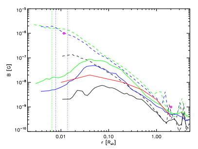
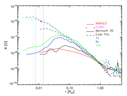
Figure 17: The magnetic field profiles for a resolution study of our cluster. Solid lines are obtained with the Bsmooth SPH-MHD implementation, dashed lines are for using Euler Potentials. The different line colors indicating different resolution. Right panel shows the same but normalizing all the profiles in the outer part of the cluster. Results taken from Dubois & Teyssier (2008) (red line) and Brüggen et al. (2005) (diamonds) are also shown.

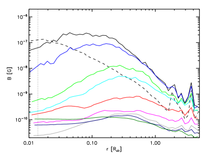
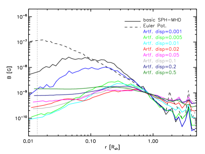
Figure 18: The magnetic field profiles obtained for the galaxy cluster using different values of the artificial dissipation. In addition the results using the Euler Potentials and the Basic MHD implementation are shown. Right panel shows the same with profiles normalized in the outer part of the cluster.

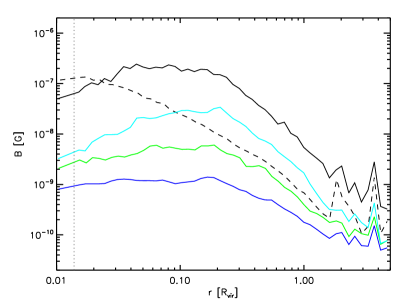
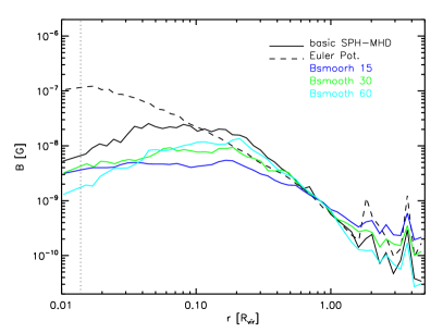
Figure 19: The magnetic field profiles obtained for the galaxy cluster using different time intervals for the smoothing procedure. In Addition the results for using the Euler Potentials and the Basic MHD implementation are shown. Right panel shows the same with profiles normalized in the outer part of the cluster.

The situation changes when using artificial magnetic dissipation, as shown in figure 18. The left panel shows the magnetic field profiles for several values of $\alpha_{B}$ compared with the profiles for the basic SPH-MHD run and that using Euler Potentials. Clearly a normal value for artificial magnetic dissipation leads to a large dissipation of magnetic field over the simulation time (e.g. close to the Hubble time). The right panels show the profiles artificially normalized at large radius. Clearly the self similarity of the profiles is lost. Therefore it appears that the use of artificially dissipation as a regularization scheme is not a good choice for cosmological simulations. Additionally it points out that true physical dissipation might play an important role in determining the shape of the magnetic field profile in galaxy clusters. Here, transport processes, cosmic rays, turbulence (especially at unresolved scales) and reconnection of magnetic field lines are not well understood, especially within the ICM. As the micro-physical origin of most of them are far outside the scales which can be ever reached by cosmological simulations, future work will have to include them as approximative, sub-grid models, possibly motivated by small scale numerical experiments.

5 Conclusions

We presented the implementation of MHD in the cosmological, SPH code GADGET. We performed various test problems and discussed several instability correction and regularization schemes. We also demonstrated the application to cosmological simulations, the role of resolution and the role the regularization schemes play in cosmological simulations.

Our main findings are:

• The combination of many improvements in the SPH implementation, like the correction terms for the variable smoothing length (Springel & Hernquist, 2002) as well as the usage of the signal velocity in the artificial viscosity (Monaghan, 1997) together with its generalization to the MHD case (Price & Monaghan, 2004a) improve the handling of magnetic fields in SPH significantly.

• Correcting the instability by explicitly subtracting the contribution of a numerical non-zero divergence of the magnetic field to the Lorenz force from the Maxwell tensor as suggested by Børve et al. (2001) seems to perform well. Specifically in three dimensional setups where it seems to work much better than other suggestions in the literature.

• The SPH-MHD implementation performs very well on simple shock tube tests as well as on planar test problems. We performed all tests in a fully three-dimensional setup and find excellent agreement of the results obtained with the SPH-MHD implementation compared to the results obtained with ATHENA in one or two dimensions.

• With a convergence study we demonstrate that the SPH-MHD results when increasing the resolution are converging to the true solution, especially in the sharp features. However, in some regions it seems that small but systematic differences converge only very slowly to the correct solution.

• Regularization schemes help to further suppresses noise and $\mathrm{div}(\vec{B})$ errors in the test simulations, however one has to carefully select the numerical parameters to avoid too strong smoothing of sharp features. Performing a full set of individual shock tube tests allows one to tune the numerical schemes and to determine optimal values. However they reflect an optimal choice for problems where the local timescales are mostly similar to the global timescale of the problem. For cosmological simulations it turns out that regularization by artificial dissipation leads to questionable results, whereas the regularization by smoothing the magnetic field (which is applied on global timescales) produces reasonable results.

• The SPH-MHD implementation allows us to perform challenging cosmological simulations, covering a large dynamical range in length-scales. For galaxy clusters, only the shape of the predicted magnetic profiles is, (with the exception of the central part of clusters) converged in resolution and in good agreement with previous studies. Also the structures obtained in synthetic Faraday Rotation maps are in good agreement with previous findings and compare well with observations.

The results obtained with artificial dissipation in cosmological simulations indicate that physical dissipation could play a crucial role in determining the exact shape of the predicted, magnetic field profiles in galaxy clusters. Future work, especially when including more physical processes at work in galaxy cluster – as can be done easily with our SPH-MHD implementation – will reveal an interesting interplay between dynamics of the cluster atmosphere and amplification of magnetic fields. Thus having the potential to shed light on many, currently unknown aspects of cluster magnetic fields, their structure and their evolution.

Appendix A Convergence

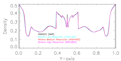
Figure 20: A cut throgh the density for the Orszang-Tang Vortex test (see Figure 13/14). Shown in black is the result obtained with Ramses, compared to the results obtained with Athena using 3 different resolutions.

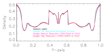
Figure 21: Same than figure 20, but showing the results obtained with the basic SPH-MHD implementation at two different resolutions compared to the results obtained with Ramses.

Numerical experiments are normally restricted by the resolution one can technically (in terms of computing/memory requirements) achieve. Therefore tests as presented in section 3 are usually at nominally better resolution than can be obtained in relevant (in this case cosmological) simulations. Never-the-less an interesting question is, how good do the numerical methods used converge if one further increase the resolution? Figure 20 and 21 show this for Athena and the basic SPH-MHD implementation respectively. We repeated the Orszang-Tang Vortex test problem with Athena on a $192^{2}$, $400^{2}$ and $800^{2}$ grid. Figure 20 shows a cut through the density of the Orszang-Tang Vortex, comparing with the result obtained with the AMR code Ramses (Teyssier, 2002). Clearly, the results obtained with Athena when increasing the resolution approaches the results obtained with Ramses. Figure 21 shows the same for setups with $350^{2}\times 5$, $700^{2}\times 5$ and $1400^{2}\times 5$ particles. The SPH-MHD implementation also converges towards the Ramses results with increasing resolution. However, although the central feature is better resolved in the SPH-MHD implementation than in the Athena run with comparable resolution, some other features can be seen to converge slower in the SPH-MHD implementation when increasing the resolution. Specifically, in some very smoothed features there are small but systematic differences between the SPH and the true solution. Here the SPH results seem to converge only extremely slowly (if at all).

References

- Balsara (1995) Balsara D. S., 1995, Journal of Computational Physics, 121, 357
- Balsara & Spicer (1999) Balsara D. S., Spicer D. D., 1999, Journal of Computational Physics, 149, 270
- Børve et al. (2001) Børve S., Omang M., Trulsen J., 2001, ApJ, 561, 82
- Børve et al. (2004) Børve S., Omang M., Trulsen J., 2004, ApJS, 153, 447
- Børve et al. (2006) Børve S., Omang M., Trulsen J., 2006, ApJ, 652, 1306
- Brio & Wu (1988) Brio M., Wu C. C., 1988, Journal of Computational Physics, 75, 500
- Brüggen et al. (2005) Brüggen M., Ruszkowski M., Simionescu A., Hoeft M., Dalla Vecchia C., 2005, ApJ, 631, L21
- Carilli & Taylor (2002) Carilli C. L., Taylor G. B., 2002, ARAA, 40, 319
- Dai & Woodward (1994) Dai W., Woodward P. R., 1994, Journal of Computational Physics, 115, 485
- Del Pra (2003) Del Pra M., 2003, Laurea Thesis
- Dolag (2000) Dolag K., 2000, in Constructing the Universe with Clusters of Galaxies Properties of Simulated Magnetized Galaxy Clusters
- Dolag et al. (1999) Dolag K., Bartelmann M., Lesch H., 1999, A&A, 348, 351
- Dolag et al. (2002) Dolag K., Bartelmann M., Lesch H., 2002, A&A, 387, 383
- Dolag et al. (2008) Dolag K., Borgani S., Murante G., Springel V., 2008, ArXiv e-prints
- Dolag et al. (2004) Dolag K., Grasso D., Springel V., Tkachev I., 2004, Soviet Journal of Experimental and Theoretical Physics Letters, 79, 583
- Dolag et al. (2005) Dolag K., Grasso D., Springel V., Tkachev I., 2005, Journal of Cosmology and Astro-Particle Physics, 1, 9
- Dolag et al. (2004) Dolag K., Jubelgas M., Springel V., Borgani S., Rasia E., 2004, ApJ, 606, L97
- Dubois & Teyssier (2008) Dubois Y., Teyssier R., 2008, A&A, 482, L13
- Enßlin et al. (2007) Enßlin T. A., Pfrommer C., Springel V., Jubelgas M., 2007, A&A, 473, 41
- Feretti et al. (1999) Feretti L., Perley R., Giovannini G., Andernach H., 1999, A&A, 341, 29
- Ferrari et al. (2008) Ferrari C., Govoni F., Schindler S., Bykov A. M., Rephaeli Y., 2008, Space Science Reviews, 134, 93
- Gingold & Monaghan (1977) Gingold R. A., Monaghan J. J., 1977, MNRAS, 181, 375
- Govoni & Feretti (2004) Govoni F., Feretti L., 2004, International Journal of Modern Physics D, 13, 1549
- Jubelgas et al. (2004) Jubelgas M., Springel V., Dolag K., 2004, MNRAS, 351, 423
- Katz & White (1993) Katz N., White S. D. M., 1993, ApJ, 412, 455
- Kulsrud et al. (1997) Kulsrud R. M., Cen R., Ostriker J. P., Ryu D., 1997, ApJ, 480, 481
- Li et al. (2008) Li S., Li H., Cen R., 2008, ApJS, 174, 1
- Londrillo & Del Zanna (2000) Londrillo P., Del Zanna L., 2000, ApJ, 530, 508
- Lucy (1977) Lucy L. B., 1977, AJ, 82, 1013
- Monaghan (1992) Monaghan J. J., 1992, ARAA, 30, 543
- Monaghan (1997) Monaghan J. J., 1997, Journal of Computational Physics, 136, 298
- Monaghan (2000) Monaghan J. J., 2000, J. Comput. Phys., 159, 290
- Monaghan (2002) Monaghan J. J., 2002, MNRAS, 335, 843
- Monaghan & Lattanzio (1985) Monaghan J. J., Lattanzio J. C., 1985, A&A, 149, 135
- Morris & Monaghan (1997) Morris J. P., Monaghan J. J., 1997, Journal of Computational Physics, 136, 41
- Omang et al. (2006) Omang M., Børve S., Trulsen J., 2006, Journal of Computational Physics, 213, 391
- Orzang & Tang (1979) Orzang S. A., Tang C. M., 1979, Journal of Fluid Mechanics, 90, 128
- Pfrommer et al. (2007) Pfrommer C., Enßlin T. A., Springel V., Jubelgas M., Dolag K., 2007, MNRAS, 378, 385
- Phillips & Monaghan (1985) Phillips G. J., Monaghan J. J., 1985, MNRAS, 216, 883
- Picone & Dahlburg (1991) Picone J. M., Dahlburg R. B., 1991, Physics of Fluids B, 3, 29
- Price & Monaghan (2004a) Price D. J., Monaghan J. J., 2004a, MNRAS, 348, 123
- Price & Monaghan (2004b) Price D. J., Monaghan J. J., 2004b, MNRAS, 348, 139
- Price & Monaghan (2005) Price D. J., Monaghan J. J., 2005, MNRAS, 364, 384
- Quinn et al. (1997) Quinn T., Katz N., Stadel J., Lake G., 1997, ArXiv Astrophysics e-prints
- Rordorf et al. (2004) Rordorf C., Grasso D., Dolag K., 2004, Astroparticle Physics, 22, 167
- Rosswog & Price (2007) Rosswog S., Price D., 2007, MNRAS, 379, 915
- Ryu & Jones (1995) Ryu D., Jones T. W., 1995, ApJ, 442, 228
- Ryu et al. (1998) Ryu D., Kang H., Biermann P. L., 1998, A&A, 335, 19
- Ryu et al. (2008) Ryu D., Kang H., Cho J., Das S., 2008, Science, 320, 909
- Sigl et al. (2004) Sigl G., Miniati F., Enssßlin T. A., 2004, Phys. Rev. D, 70, 043007
- Sijacki & Springel (2006) Sijacki D., Springel V., 2006, MNRAS, 371, 1025
- Springel (2005) Springel V., 2005, MNRAS, 364, 1105
- Springel & Hernquist (2002) Springel V., Hernquist L., 2002, MNRAS, 333, 649
- Springel & Hernquist (2003) Springel V., Hernquist L., 2003, MNRAS, 339, 289
- Springel et al. (2001) Springel V., White M., Hernquist L., 2001, ApJ, 549, 681
- Steinmetz (1996) Steinmetz M., 1996, in IAU Symp. 171: New Light on Galaxy Evolution Mergers and Formation of Disk Galaxies in Hierarchically Clustering Universes. p. 259
- Stone et al. (2008) Stone J. M., Gardiner T. A., Teuben P., Hawley J. F., Simon J. B., 2008, ArXiv e-prints, 804
- Teyssier (2002) Teyssier R., 2002, A&A, 385, 337
- Tormen et al. (1997) Tormen G., Bouchet F. R., White S. D. M., 1997, MNRAS, 286, 865
- Tornatore et al. (2007) Tornatore L., Borgani S., Dolag K., Matteucci F., 2007, MNRAS, 382, 1050
- Tornatore et al. (2004) Tornatore L., Borgani S., Matteucci F., Recchi S., Tozzi P., 2004, MNRAS, 349, L19
- Tóth (2000) Tóth G., 2000, Journal of Computational Physics, 161, 605
- White (1996) White S. D. M., 1996, in Schaeffer R., Silk J., Spiro M., Zinn-Justin J., eds, Cosmology and Large Scale Structure Formation and Evolution of Galaxies. pp 349–+
- Yoshida et al. (2001) Yoshida N., Sheth R. K., Diaferio A., 2001, MNRAS, 328, 669