Stabilizer Quantum Codes: A Unified View
based on Forney-style Factor Graphs

Abstract

Quantum error-correction codes (QECCs) are a vital ingredient of quantum computation and communication systems. In that context it is highly desirable to design QECCs that can be represented by graphical models which possess a structure that enables efficient and close-to-optimal iterative decoding.

In this paper we focus on stabilizer QECCs, a class of QECCs whose construction is rendered non-trivial by the fact that the stabilizer label code, a code that is associated with a stabilizer QECC, has to satisfy a certain self-orthogonality condition. In order to design graphical models of stabilizer label codes that satisfy this condition, we extend a duality result for Forney-style factor graphs (FFGs) to the stabilizer label code framework. This allows us to formulate a simple FFG design rule for constructing stabilizer label codes, a design rule that unifies several earlier stabilizer label code constructions.

I Introduction

Graphical models have played a very important role in the recent history of error-correction coding (ECC) schemes for conventional channel and storage setups [1]. In particular, some of the most powerful ECC schemes known today, like message-passing iterative (MPI) decoding of low-density parity-check (LDPC) and turbo codes, can be represented by graphical models. It is therefore highly desirable to extend the design and analysis lessons that have been learned from these ECC systems to quantum error-correction code (QECC) systems, in particular to stabilizer QECC systems.

For background material and a history of stabilizer QECCs in particular, and quantum information processing (QIP) in general, we refer to the excellent textbook by Nielsen and Chuang [2]. Alternatively, one can consult some early papers on stabilizer QECCs, e.g. [3, 4], or more recent accounts, e.g. [5, 6, 7]. The aim of the present paper is to introduce a Forney-style factor graph (FFG) framework that allows one to construct FFGs that represent interesting classes of stabilizer QECCs, more precisely, that represent interesting classes of stabilizer label codes and normalizer label codes. Anyone familiar with the basics of stabilizer QECCs can then easily formulate the corresponding stabilizer QECCs. (Note that due to space constraints this paper does not motivate stabilizer QECCs and does not define them. However, the paper does not use any QIP jargon and should therefore be accessible to anyone familiar with the basics of coding theory.)

This paper is structured as follows. In Section II we introduce the basics on FFGs and in Section III we extend a well-known duality result for FFGs. In Section IV we then show how this duality result can be used to construct stabilizer and normalizer label codes. Afterwards, in Section V we discuss several examples of such codes, in particular we show that our FFG framework unifies earlier proposed code constructions. We conclude by briefly commenting on message-passing iterative decoding and linear programming decoding in Section VI. Because of space limitations we decided to formulate many of the concepts and results in terms of examples; most of them can be suitably generalized.

Our notation is quite standard. In particular, the field of real numbers will be denoted by $\mathbb{R}$ and the ring of integers modulo $p$ by $\mathbb{Z}_{p}$. (If $p$ is a prime, then $\mathbb{Z}_{p}$ is a field.) The Galois field $\mathbb{F}_{4}$ will be based on the set $\{0,1,\omega,\omega^{2}\}$, where $\omega$ satisfies $\omega^{2}=\omega+1$ (and therefore also $\omega^{3}=1$), and where conjugation is defined by $\overline{x}=x^{2}$. Moreover, for any statement $S$ we will use Iverson’s convention which says that $[S]=1$ if $S$ is true and $[S]=0$ otherwise.

II Forney-style Factor Graphs (FFGs)

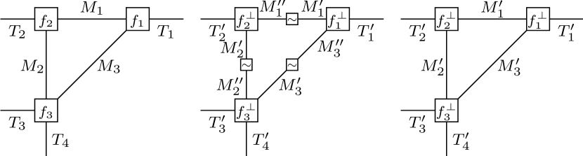
Figure 1: Left: A simple FFG. Middle: Dual of the FFG on the left. Right: Dual of the FFG on the left if alphabet groups have characteristic $2$.

FFGs [8, 9, 1], also known as normal factor graphs, are graphs that represent multivariate functions. For example, let $\mathsf{T}=4$ and $\mathsf{M}=3$, let $\mathcal{T}_{i}$, $i=1,\ldots,\mathsf{T}$ and $\mathcal{M}_{i}$, $i=1,\ldots,\mathsf{M}$ be some arbitrary alphabets, and consider the function $f:\ \prod_{i=1}^{\mathsf{T}}\mathcal{T}_{i}\times\prod_{i=1}^{\mathsf{M}}\mathcal{M}_{i}\ \to\ \mathbb{R}$ that represents the mapping

$$(\mathbf{t},\mathbf{m})\mapsto f_{1}(t_{1},m_{1},m_{3})\,f_{2}(t_{2},m_{1},m_{2})\,f_{3}(t_{3},t_{4},m_{2},m_{3}).$$

Here, $f$ is called the global function and is the product of $\mathsf{F}$ functions $f_{i}$, $i=1,\ldots,\mathsf{F}$ (here $\mathsf{F}=3$), which are called local functions. Whereas the argument set of the function $f$ encompasses $t_{1}$, $t_{2}$, $t_{3}$, $t_{4}$, $m_{1}$, $m_{2}$, and $m_{3}$, the function $f_{1}$ has only $t_{1}$, $m_{1}$, and $m_{3}$ as arguments, $f_{2}$ has only $t_{2}$, $m_{1}$, and $m_{2}$ as arguments, and $f_{3}$ has only $t_{3}$, $t_{4}$, $m_{2}$, and $m_{3}$ as arguments. Graphically, we represent this function decomposition as follows, cf. Fig. 1 (left):

• For each local function we draw a function node (vertex).

• For each variable we draw an half-edge or an edge.

• If a variable appears as an argument in only one local function then we draw an half-edge that is connected to that local function. If a variable appears as an argument in two local functions then we draw an edge that connects these two local functions.

In our example the variables that are associated with half-edges are labeled $T_{i}$, $i=1,\ldots,\mathsf{T}$, whereas the variables that are associated with edges are labeled $M_{i}$, $i=1,\ldots,\mathsf{M}$. This distinction of variable labels will be very helpful later on when we will dualize the global function.

Interesting are global functions where the local function argument sets are strict subsets of the global function argument set: the fewer arguments appear in the local functions, the sparser the corresponding FFG will be.

Consider again the FFG in Figure 1 (left) and let the local functions represent indicator functions, i.e.,

$$f_{1}(t_{1},m_{1},m_{3}) \triangleq\big{[}(t_{1},m_{1},m_{3})\in\mathcal{C}_{1}\big{]},$$

$$f_{2}(t_{2},m_{1},m_{2}) \triangleq\big{[}(t_{2},m_{1},m_{2})\in\mathcal{C}_{2}\big{]},$$

$$f_{3}(t_{3},t_{4},m_{2},m_{3}) \triangleq\big{[}(t_{3},t_{4},m_{2},m_{3})\in\mathcal{C}_{3}\big{]},$$

for some codes $\mathcal{C}_{1}\subseteq\mathcal{T}_{1}\times\mathcal{M}_{1}\times\mathcal{M}_{3}$, $\mathcal{C}_{2}\subseteq\mathcal{T}_{2}\times\mathcal{M}_{1}\times\mathcal{M}_{2}$, and $\mathcal{C}_{3}\subseteq\mathcal{T}_{3}\times\mathcal{T}_{4}\times\mathcal{M}_{2}\times\mathcal{M}_{3}$. The restriction of the resulting global function to the variables $\mathbf{t}$, i.e., to the variables that are associated with the half-edges, yields the function $[\mathbf{t}\in\mathcal{C}]$ with

$$\mathcal{C}=\left\{\mathbf{t}\in\prod_{i=1}^{\mathsf{T}}\mathcal{T}_{i}\ \left|\ \begin{array}[]{c}\text{there exists an $\mathbf{m}$}\\ \text{such that $f(\mathbf{t},\mathbf{m})=1$}\end{array}\right.\right\}\;.$$

Clearly, if the sets $\mathcal{T}_{i}$, $i=1,\ldots,\mathsf{T}$, and $\mathcal{M}_{i}$, $i=1,\ldots,\mathsf{M}$, are groups and the codes $\mathcal{C}_{i}$, $i=1,\ldots,\mathsf{F}$ are group codes then $\mathcal{C}$ is a group code.

III Dualizing FFGs

In the context of stabilizer QECCs, dual codes (under the symplectic inner product) play a very important role. The aim of this section is to start with an FFG that represents the indicator function of some code and to construct an FFG that represents the indicator function of the dual of that code. To that end we will heavily use insights from [8, Section VII] on Pontryagin duality theory in the context of FFGs, notably one of relatively few results that hold for graphical models without and with cycles.

For the rest of the paper, we make the following definitions.

Definition 1

Let $p$ be some prime.

For $i=1,\ldots,\mathsf{T}$:

• We define $\mathcal{T}_{i}$ to be the group $\mathbb{Z}_{p}^{2}$ with vector addition modulo $p$ and we denote elements of $\mathcal{T}_{i}$ by $t_{i}=(t_{X,i},t_{Z,i})$.

• We let $\mathcal{T}^{\prime}_{i}$ be the character group of $\mathcal{T}_{i}$. Because $\mathcal{T}^{\prime}_{i}$ turns out to be isomorphic to $\mathcal{T}_{i}$, we identify $\mathcal{T}^{\prime}_{i}$ with $\mathcal{T}_{i}$. Elements of $\mathcal{T}^{\prime}_{i}$ will be denoted by $t^{\prime}_{i}=(t^{\prime}_{X,i},t^{\prime}_{Z,i})$.

• We define the inner product $\langle t_{i},t^{\prime}_{i}\rangle:\ \mathcal{T}_{i}\times\mathcal{T}^{\prime}_{i}\to\mathbb{Z}_{p}$ to be the symplectic inner product, i.e.,

  $$\langle t_{i},t^{\prime}_{i}\rangle \triangleq\begin{bmatrix}t_{X,i}\\ t_{Z,i}\end{bmatrix}^{\mathrm{T}}\!\!\!\cdot\begin{bmatrix}0&1\\ 1&0\end{bmatrix}\cdot\begin{bmatrix}t^{\prime}_{X,i}\\ t^{\prime}_{Z,i}\end{bmatrix}=t_{X,i}t^{\prime}_{Z,i}+t_{Z,i}t^{\prime}_{X,i}\,,$$

  where ^T represents vector transposition and where addition and multiplication are modulo $p$. (Note that we are using angular brackets to denote inner products. This is in contrast to [8] that used angular brackets to denote pairings, which are exponential functions of inner products.)

For $i=1,\ldots,\mathsf{M}$:

• We let $\mu_{i}$ be some positive integer, we define $\mathcal{M}_{i}$ to be the group $(\mathbb{Z}_{p}^{2})^{\mu_{i}}$ with vector addition modulo $p$, and we denote elements of $\mathcal{M}_{i}$ by $m_{i}=\bigl{(}(m_{X,i,1},m_{Z,i,1}),\ldots,(m_{X,i,\mu_{i}},m_{Z,i,\mu_{i}})\bigr{)}$.

• We let $\mathcal{M}^{\prime}_{i}$ denote the character group of $\mathcal{M}_{i}$. Again, because $\mathcal{M}^{\prime}_{i}$ turns out to be isomorphic to $\mathcal{M}_{i}$, we identify $\mathcal{M}^{\prime}_{i}$ with $\mathcal{M}_{i}$. Elements of $\mathcal{M}^{\prime}_{i}$ will be denoted by $m^{\prime}_{i}=\bigl{(}(m^{\prime}_{X,i,1},m^{\prime}_{Z,i,1}),\ldots,(m^{\prime}_{X,i,\mu_{i}},m^{\prime}_{Z,i,\mu_{i}})\bigr{)}$.

• We define the inner product $\langle m_{i},m^{\prime}_{i}\rangle$ to be the symplectic inner product, i.e.,

  $$\langle m_{i},m^{\prime}_{i}\rangle$$

  $$\triangleq\begin{bmatrix}m_{X,i,1}\\ m_{Z,i,1}\\ \vdots\\ m_{X,i,\mu_{i}}\\ m_{Z,i,\mu_{i}}\end{bmatrix}^{\mathrm{T}}\!\!\!\cdot\begin{bmatrix}0&1&&&\\ 1&0&&&\\ &&\ddots&&&\\ &&&0&1\\ &&&1&0\end{bmatrix}\cdot\begin{bmatrix}m^{\prime}_{X,i,1}\\ m^{\prime}_{Z,i,1}\\ \vdots\\ m^{\prime}_{X,i,\mu_{i}}\\ m^{\prime}_{Z,i,\mu_{i}}\end{bmatrix}$$

  $$=\sum_{h=1^{\prime}}^{\mu_{i}}\big{(}m_{X,i,h}m^{\prime}_{Z,i,h}+m_{Z,i,h}m^{\prime}_{X,i,h}\big{)}\;.$$

The above inner products induce inner products on vectors, e.g., $\langle\mathbf{t},\mathbf{t}^{\prime}\rangle:\ \prod_{i=1}^{\mathsf{T}}\mathcal{T}_{i}\times\prod_{i=1}^{\mathsf{T}}\mathcal{T}^{\prime}_{i}\to\mathbb{Z}_{p}$ is the inner product defined by $\langle\mathbf{t},\mathbf{t}^{\prime}\rangle\triangleq\sum_{i=1}^{\mathsf{T}}\langle t_{i},t^{\prime}_{i}\rangle$, etc..

Moreover, all codes are assumed to be group codes. $\square$

In the following, because of the natural isomorphism of the groups $(\mathbb{Z}_{p}^{2})^{n}$ and $(\mathbb{Z}_{p}^{n})^{2}$, a vector $\mathbf{t}\in(\mathbb{Z}_{p}^{2})^{n}$ will not only be written as

$$\mathbf{t} =\big{(}(t_{X,1},t_{Z,1}),\ldots,(t_{X,n},t_{Z,n})\big{)}$$

but also as

$$\mathbf{t}=(\mathbf{t}_{X},\mathbf{t}_{Z})\ \text{ with }\ \mathbf{t}_{X} =(t_{X,1},\ldots,t_{X,n})\in\mathbb{Z}_{p}^{n}\;,$$

$$\mathbf{t}_{Z} =(t_{Z,1},\ldots,t_{Z,n})\in\mathbb{Z}_{p}^{n}\;.$$

With this convention, the symplectic inner product of $\mathbf{t}$ and $\mathbf{t}^{\prime}$ can be written as

$$\langle\mathbf{t},\mathbf{t}^{\prime}\rangle \triangleq\begin{bmatrix}t_{X,1}\\ t_{Z,1}\\ \vdots\\ t_{X,n}\\ t_{Z,n}\end{bmatrix}^{\mathrm{T}}\!\!\!\cdot\begin{bmatrix}0&1&&&\\ 1&0&&&\\ &&\ddots&&&\\ &&&0&1\\ &&&1&0\end{bmatrix}\cdot\begin{bmatrix}t^{\prime}_{X,1}\\ t^{\prime}_{Z,1}\\ \vdots\\ t^{\prime}_{X,n}\\ t^{\prime}_{Z,n}\end{bmatrix}$$

or as

$$\langle\mathbf{t},\mathbf{t}^{\prime}\rangle =\begin{bmatrix}\mathbf{t}_{X}^{\mathrm{T}}\\ \mathbf{t}_{Z}^{\mathrm{T}}\end{bmatrix}^{\mathrm{T}}\!\!\!\cdot\begin{bmatrix}\mathbf{0}&\mathbb{1}_{n}\\ \mathbb{1}_{n}&\mathbf{0}\end{bmatrix}\cdot\begin{bmatrix}(\mathbf{t}^{\prime}_{X})^{\mathrm{T}}\\ (\mathbf{t}^{\prime}_{Z})^{\mathrm{T}}\end{bmatrix}$$

$$=\mathbf{t}_{X}\cdot(\mathbf{t}^{\prime}_{Z})^{\mathrm{T}}+\mathbf{t}_{Z}\cdot(\mathbf{t}^{\prime}_{X})^{\mathrm{T}}\;,$$

where $\mathbb{1}_{n}$ is the $n\times n$ identity matrix. Similar expressions will also be used for the vector $\mathbf{m}$ and combinations of $\mathbf{t}$ and $\mathbf{m}$.

Definition 2

The dual code $\mathcal{C}^{\perp}$ (under the symplectic inner product) of some group code $\mathcal{C}\subseteq\prod_{i=1}^{\mathsf{T}}\mathcal{T}_{i}$ is defined to be

$$\mathcal{C}^{\perp} \triangleq\left\{\left.\mathbf{t}^{\prime}\in\prod_{i=1}^{\mathsf{T}}\mathcal{T}^{\prime}_{i}\ \right|\ \langle\mathbf{t},\mathbf{t}^{\prime}\rangle=0\right\}\;.$$

$\square$

Note that $\mathcal{C}^{\perp}$ is also a group code and that $(\mathcal{C}^{\perp})^{\perp}=\mathcal{C}$. Similarly, for any $i=1,\ldots,\mathsf{T}$, because $\mathcal{C}_{i}$ was assumed to be a group code, we can define its dual $\mathcal{C}_{i}^{\perp}$.

In the following, we want to show that there is an FFG representing $\mathcal{C}^{\perp}$ that is tightly related to the FFG that represents $\mathcal{C}$. Continuing our example from Section II, let $\mathcal{M}^{\prime\prime}_{i}\triangleq\mathcal{M}^{\prime}_{i}$ for $i=1,\ldots,\mathsf{M}$, and let $f^{\perp}:\ \prod_{i=1}^{\mathsf{T}}\mathcal{T}^{\prime}_{i}\times\prod_{i=1}^{\mathsf{M}}\mathcal{M}^{\prime}_{i}\times\prod_{i=1}^{\mathsf{M}}\mathcal{M}^{\prime\prime}_{i}\ \to\ \mathbb{R}$ be the function that represents the mapping

$$(\mathbf{t}^{\prime},\mathbf{m}^{\prime},\mathbf{m}^{\prime\prime})\mapsto f^{\perp}_{1}(t^{\prime}_{1},m^{\prime}_{1},m^{\prime\prime}_{3})\ f^{\perp}_{2}(t^{\prime}_{2},m^{\prime\prime}_{1},m^{\prime}_{2})$$

$$\cdot\,f^{\perp}_{3}(t^{\prime}_{3},t^{\prime}_{4},m^{\prime\prime}_{2},m^{\prime}_{3})$$

$$\cdot\,\big{[}m^{\prime}_{1}{=}-m^{\prime\prime}_{1}\big{]}\,\big{[}m^{\prime}_{2}{=}-m^{\prime\prime}_{2}\big{]}\,\big{[}m^{\prime}_{3}{=}-m^{\prime\prime}_{3}\big{]}$$

with

$$f^{\perp}_{1}(t^{\prime}_{1},m^{\prime}_{1},m^{\prime\prime}_{3}) \triangleq\big{[}(t^{\prime}_{1},m^{\prime}_{1},m^{\prime\prime}_{3})\in\mathcal{C}^{\perp}_{1}\big{]}\;,$$

$$f^{\perp}_{2}(t^{\prime}_{2},m^{\prime\prime}_{1},m^{\prime}_{2}) \triangleq\big{[}(t^{\prime}_{2},m^{\prime\prime}_{1},m^{\prime}_{2})\in\mathcal{C}^{\perp}_{2}\big{]}\;,$$

$$f^{\perp}_{3}(t^{\prime}_{3},t^{\prime}_{4},m^{\prime\prime}_{2},m^{\prime}_{3}) \triangleq\big{[}(t^{\prime}_{3},t^{\prime}_{4},m^{\prime\prime}_{2},m^{\prime}_{3})\in\mathcal{C}^{\perp}_{3}\big{]}\;.$$

The function $f^{\perp}$ is depicted by the FFG in Figure 1 (middle) where the function nodes with a tilde in them represent the indicator functions $[m^{\prime}_{1}{=}-m^{\prime\prime}_{1}]$, $[m^{\prime}_{2}{=}-m^{\prime\prime}_{2}]$, and $[m^{\prime}_{3}{=}-m^{\prime\prime}_{3}]$, respectively. With this, we can follow [8] and establish the next theorem.

Theorem 3

With the above definitions,

$$\mathcal{C}^{\perp} =\left\{\left.\mathbf{t}^{\prime}\in\prod_{i=1}^{\mathsf{T}}\mathcal{T}^{\prime}_{i}\ \right|\ \begin{array}[]{c}\text{there exists $\mathbf{m}^{\prime}$ and $\mathbf{m}^{\prime\prime}$}\\ \text{such that $f^{\perp}(\mathbf{t}^{\prime},\mathbf{m}^{\prime},\mathbf{m}^{\prime\prime})=1$}\end{array}\right\}\;.$$

Proof.

(The proof is for the example code in Figure 1, but the proof can easily be generalized.) Let $\mathbf{t}^{\prime}\in\prod_{i=1}^{\mathsf{T}}\mathcal{T}^{\prime}_{i}$ be such that there exist $\mathbf{m}^{\prime}$ and $\mathbf{m}^{\prime\prime}$ such that $f^{\perp}(\mathbf{t},\mathbf{m}^{\prime},\mathbf{m}^{\prime\prime})=1$. Moreover, let $\mathbf{t}\in\mathcal{C}$ and let $\mathbf{m}$ be such that $f(\mathbf{t},\mathbf{m})=1$. Then,

$$\langle\mathbf{t},\mathbf{t}^{\prime}\rangle =\sum_{i=1}^{\mathsf{T}}\langle t_{i},t^{\prime}_{i}\rangle$$

$$=\sum_{i=1}^{\mathsf{T}}\langle t_{i},t^{\prime}_{i}\rangle+\sum_{i=1}^{\mathsf{M}}\langle m_{i},m^{\prime}_{i}\rangle-\sum_{i=1}^{\mathsf{M}}\langle m_{i},m^{\prime}_{i}\rangle$$

$$=\sum_{i=1}^{\mathsf{T}}\langle t_{i},t^{\prime}_{i}\rangle+\sum_{i=1}^{\mathsf{M}}\langle m_{i},m^{\prime}_{i}\rangle+\sum_{i=1}^{\mathsf{M}}\langle m_{i},m^{\prime\prime}_{i}\rangle$$

$$=\big{(}\langle t_{1},t^{\prime}_{1}\rangle+\langle m_{1},m^{\prime}_{1}\rangle+\langle m_{3},m^{\prime\prime}_{3}\rangle\big{)}+$$

$$\quad\ \big{(}\langle t_{2},t^{\prime}_{2}\rangle+\langle m_{1},m^{\prime\prime}_{1}\rangle+\langle m_{2},m^{\prime}_{2}\rangle\big{)}+$$

$$\quad\ \big{(}\langle t_{3},t^{\prime}_{3}\rangle+\langle t_{4},t^{\prime}_{4}\rangle+\langle m_{2},m^{\prime\prime}_{2}\rangle+\langle m_{3},m^{\prime}_{3}\rangle\big{)}$$

$$\overset{(*)}{=}0+0+0=0\;.$$

Here, step $(*)$ follows from the fact that $(t_{1},m_{1},m_{3})\in\mathcal{C}_{1}$ and $(t^{\prime}_{1},m^{\prime}_{1},m^{\prime\prime}_{3})\in\mathcal{C}^{\perp}_{1}$ imply that $\langle t_{1},t^{\prime}_{1}\rangle+\langle m_{1},m^{\prime}_{1}\rangle+\langle m_{3},m^{\prime\prime}_{3}\rangle=0$, with similar expressions for the other subcodes.

We see that $\mathbf{t}^{\prime}$ is orthogonal to $\mathbf{t}$, and because $\mathbf{t}\in\mathcal{C}$ was arbitrary, $\mathbf{t}^{\prime}$ must be in $\mathcal{C}^{\perp}$. ∎

Assumption 4

For the rest of the paper we will assume that $p=2$, which implies that the groups $\mathcal{T}_{i}$, $\mathcal{T}^{\prime}_{i}$, $i=1,\ldots,\mathsf{T}$, and the groups $\mathcal{M}_{i}$, $\mathcal{M}^{\prime}_{i}$, $\mathcal{M}^{\prime\prime}_{i}$, $i=1,\ldots,\mathsf{M}$, have characteristic $2$. Therefore, $m^{\prime\prime}_{i}=-m^{\prime\prime}_{i}$ for all $m^{\prime\prime}_{i}\in\mathcal{M}^{\prime\prime}_{i}$, $i=1,\ldots,\mathsf{M}$, etc..

So, given that we are only interested in arguments of $f^{\perp}$ that lead to non-zero function values, any valid configuration $(\mathbf{t}^{\prime},\mathbf{m}^{\prime},\mathbf{m}^{\prime\prime})$ of the FFG in Figure 1 (middle) fulfills $\mathbf{m}^{\prime}=-\mathbf{m}^{\prime\prime}=\mathbf{m}^{\prime\prime}$. This observation allows us to simplify the function $f^{\perp}$ to $f^{\perp}:\ \prod_{i=1}^{\mathsf{T}}\mathcal{T}^{\prime}_{i}\times\prod_{i=1}^{\mathsf{M}}\mathcal{M}^{\prime}_{i}\ \to\ \mathbb{R}$ that represents the mapping

$$(\mathbf{t}^{\prime},\mathbf{m}^{\prime})\mapsto f^{\perp}_{1}(t^{\prime}_{1},m^{\prime}_{1},m^{\prime}_{3})f^{\perp}_{2}(t^{\prime}_{2},m^{\prime}_{1},m^{\prime}_{2})f^{\perp}_{3}(t^{\prime}_{3},t^{\prime}_{4},m^{\prime}_{2},m^{\prime}_{3})$$

with

$$f^{\perp}_{1}(t^{\prime}_{1},m^{\prime}_{1},m^{\prime}_{3}) \triangleq\big{[}(t^{\prime}_{1},m^{\prime}_{1},m^{\prime}_{3})\in\mathcal{C}^{\perp}_{1}\big{]}\;,$$

$$f^{\perp}_{2}(t^{\prime}_{2},m^{\prime}_{1},m^{\prime}_{2}) \triangleq\big{[}(t^{\prime}_{2},m^{\prime}_{1},m^{\prime}_{2})\in\mathcal{C}^{\perp}_{2}\big{]}\;,$$

$$f^{\perp}_{3}(t^{\prime}_{3},t^{\prime}_{4},m^{\prime}_{2},m^{\prime}_{3}) \triangleq\big{[}(t^{\prime}_{3},t^{\prime}_{4},m^{\prime}_{2},m^{\prime}_{3})\in\mathcal{C}^{\perp}_{3}\big{]}\;.$$

The new function $f^{\perp}$ is depicted by the FFG in Figure 1 (right). It is clear that Theorem 3 simplifies to the following corollary.

Corollary 5

With the above definitions and Assumption 4 we have

$$\mathcal{C}^{\perp} =\left\{\left.\mathbf{t}^{\prime}\in\prod_{i=1}^{\mathsf{T}}\mathcal{T}^{\prime}_{i}\ \right|\ \begin{array}[]{c}\text{there exists an $\mathbf{m}^{\prime}$}\\ \text{such that $f^{\perp}(\mathbf{t}^{\prime},\mathbf{m}^{\prime})=1$}\end{array}\right\}\;.$$

Proof.

Follows easily from Theorem 3. ∎

We conclude this section with a definition that will be crucial for the remainder of this paper, namely self-orthogonality and self-duality (under the symplectic inner product) of a code.

Definition 6

Let $\mathcal{C}$ be a group code with dual code $\mathcal{C}^{\perp}$. Then,

• $\mathcal{C}$ is called self-orthogonal if $\mathcal{C}\subseteq\mathcal{C}^{{\perp}}$ and

• $\mathcal{C}$ is called self-dual if $\mathcal{C}=\mathcal{C}^{\perp}$.

(Note that a code $\mathcal{C}$ is self-orthogonal if $\langle\mathbf{t},\mathbf{t}^{\prime}\rangle=0$ for all $\mathbf{t},\mathbf{t}^{\prime}\in\mathcal{C}$.) $\square$

IV Stabilizer Label Codes and
Normalizer Label Codes

Let $\mathcal{C}$ be a code over $\mathbb{Z}_{2}^{2}$ that is self-orthogonal under the symplectic inner product. Without going into the details of the stabilizer QECC framework, such a code $\mathcal{C}$ can be used to construct a stabilizer QECC. In that context, the codes $\mathcal{C}$ and $\mathcal{C}^{\perp}$ are called, respectively, the stabilizer label code and the normalizer label code associated with that stabilizer QECC.

Proposition 7

Using the notation that has been introduced so far, in particular Definition 1 and Assumption 4, let $\mathcal{C}\subseteq\prod_{i=1}^{\mathsf{T}}\mathcal{T}_{i}$ be a group code whose indicator function is defined by an FFG containing half-edges $T_{i}$, $i=1,\ldots,\mathsf{T}$, full edges $M_{i}$, $i=1,\ldots,\mathsf{M}$, and function nodes $f_{i}$, $i=1,\ldots,\mathsf{F}$, where the latter are indicator functions of group codes $\mathcal{C}_{i}$, $i=1,\ldots,\mathsf{F}$. Then,

• $\mathcal{C}$ is self-orthogonal if all $\mathcal{C}_{i}$ are self-orthogonal, and

• $\mathcal{C}$ is self-dual if all $\mathcal{C}_{i}$ are self-dual.

Proof.

First we consider the case where all $\mathcal{C}_{i}$ are self-orthogonal. The code $\mathcal{C}$ can be represented by an FFG like the FFG in Figure 1 (left). Let $\mathbf{t}$ be a codeword in $\mathcal{C}$ and let $\mathbf{m}$ be such that $f(\mathbf{t},\mathbf{m})=1$. Because of Definition 1, Assumption 4, and Corollary 5, its dual code $\mathcal{C}^{\perp}$ can be represented by an FFG like the FFG in Figure 1 (right). Then, because the FFG in Figure 1 (left) is topologically equivalent to the FFG in Figure 1 (right) and because all $\mathcal{C}_{i}$ are self-orthogonal, it follows that $f^{\perp}(\mathbf{t},\mathbf{m})=1$, which in turn yields $\mathbf{t}\in\mathcal{C}^{\perp}$. Finally, because $\mathbf{t}\in\mathcal{C}$ was arbitrary, we see that $\mathcal{C}\subseteq\mathcal{C}^{\perp}$, i.e., that $\mathcal{C}$ is self-orthogonal.

Secondly, we consider the case where all $\mathcal{C}_{i}$ are self-dual. Similarly to the above argument, we can show that $\mathcal{C}\subseteq\mathcal{C}^{\perp}$. Reversing the roles of $\mathcal{C}$ and $\mathcal{C}^{\perp}$, we can also show that $\mathcal{C}^{\perp}\subseteq\mathcal{C}$. This proves that $\mathcal{C}=\mathcal{C}^{\perp}$, i.e., that $\mathcal{C}$ is self-dual. ∎

Obviously, Proposition 7 gives us a simple tool to construct stabilizer label codes and normalizer label codes. It does not seem that duality results for FFGs, which are at the heart of Proposition 7, have been leveraged before to construct stabilizer QECCs.

IV-A CSS Codes

CSS codes are a family of stabilizer QECCs named after Calderbank, Shor, and Steane (see e.g. [2]). For these codes we will not use our formalism, however, later on CSS codes can be used as component codes for longer codes.

Let $\mathcal{B}_{1}\subseteq\mathbb{Z}_{2}^{n}$ and $\mathcal{B}_{2}\subseteq\mathbb{Z}_{2}^{n}$ be two binary codes of length $n$ such that $\mathbf{b}\cdot(\mathbf{b}^{\prime})^{\mathrm{T}}=0$ for all $\mathbf{b}\in\mathcal{B}_{1}$ and $\mathbf{b}^{\prime}\in\mathcal{B}_{2}$. Based on these two binary codes, we define the stabilizer label code

$$\mathcal{C} \triangleq\big{\{}\mathbf{t}=(\mathbf{t}_{X},\mathbf{t}_{Z})\ \big{|}\ \mathbf{t}_{X}\in\mathcal{B}_{1}\ \text{and}\ \mathbf{t}_{Z}\in\mathcal{B}_{2}\big{.}\big{\}}.$$

It can easily be seen that the code $\mathcal{C}$ is self-orthogonal. Namely, for any $\mathbf{t}=(\mathbf{t}_{X},\mathbf{t}_{Z}),\ \mathbf{t}^{\prime}=(\mathbf{t}^{\prime}_{X},\mathbf{t}^{\prime}_{Z})\in\mathcal{C}$ we have $\langle\mathbf{t},\mathbf{t}^{\prime}\rangle=\mathbf{t}_{X}\cdot(\mathbf{t}^{\prime}_{Z})^{\mathrm{T}}+\mathbf{t}_{Z}\cdot(\mathbf{t}^{\prime}_{X})^{\mathrm{T}}=0+0=0$, where $\mathbf{t}_{X}\cdot(\mathbf{t}^{\prime}_{Z})^{\mathrm{T}}=0$ follows from $\mathbf{t}_{X}\in\mathcal{B}_{1}$ and $\mathbf{t}^{\prime}_{Z}\in\mathcal{B}_{2}$, and where $\mathbf{t}_{Z}\cdot(\mathbf{t}^{\prime}_{X})^{\mathrm{T}}=\mathbf{t}^{\prime}_{X}\cdot(\mathbf{t}_{Z})^{\mathrm{T}}=0$ follows from $\mathbf{t}^{\prime}_{X}\in\mathcal{B}_{1}$ and $\mathbf{t}_{Z}\in\mathcal{B}_{2}$.

Example 8

The so-called seven qubit Steane stabilizer QECC (see e.g. [2]) is a CSS code where both $\mathcal{B}_{1}$ and $\mathcal{B}_{2}$ equal the $[7,3,4]$ binary simplex code, i.e., the code given by the rowspan of the matrix

$$\begin{bmatrix}0&0&0&1&1&1&1\\ 0&1&1&0&0&1&1\\ 1&0&1&0&1&0&1\end{bmatrix}\;.$$

$\square$

IV-B Codes over $\mathbb{F}_{4}$

Let us associate with any vector $\mathbf{t}=(\mathbf{t}_{X},\mathbf{t}_{Z})\in(\mathbb{Z}_{2}^{n})^{2}$ the vector $\mathbf{t}_{\mathbb{F}_{4}}=(t_{\mathbb{F}_{4},1},\ldots,t_{\mathbb{F}_{4},n})\in\mathbb{F}_{4}^{n}$ through the mapping

$$\mathbf{t}_{\mathbb{F}_{4}} \triangleq\gamma_{\mathbb{Z}_{2}^{2}\to\mathbb{F}_{4}}(\mathbf{t})\triangleq\omega\,\mathbf{t}_{X}+\overline{\omega}\,\mathbf{t}_{Z}\;.$$

Clearly, the mapping $\gamma_{\mathbb{Z}_{2}^{2}\to\mathbb{F}_{4}}$ is injective and surjective and therefore bijective, and so there is a bijective mapping between $\mathcal{C}$ and $\mathcal{C}_{\mathbb{F}_{4}}\triangleq\gamma_{\mathbb{Z}_{2}^{2}\to\mathbb{F}_{4}}(\mathcal{C})$, the latter being the image of $\mathcal{C}$ under the mapping $\gamma_{\mathbb{Z}_{2}^{2}\to\mathbb{F}_{4}}$. Because $\mathcal{C}$ was assumed to be a group/additive code, $\mathcal{C}_{\mathbb{F}_{4}}$ is also a group/additive code. Moreover, if for any codeword $\mathbf{t}_{\mathbb{F}_{4}}\in\mathcal{C}_{\mathbb{F}_{4}}$ it holds that $\omega\cdot\mathbf{t}_{\mathbb{F}_{4}}\in\mathcal{C}_{\mathbb{F}_{4}}$, then the code $\mathcal{C}_{\mathbb{F}_{4}}$ is a linear code, i.e., not only is the sum of two codewords again a codeword, but any $\mathbb{F}_{4}$-multiple of a codewords is also a codeword. If $\mathcal{C}_{\mathbb{F}_{4}}$ is a linear code then also $\mathcal{C}^{\perp}_{\mathbb{F}_{4}}$ is a linear code. With this, Proposition 7 can be suitably reformulated for sub-codes $\mathcal{C}_{\mathbb{F}_{4},i}\triangleq\gamma_{\mathbb{Z}_{2}^{2}\to\mathbb{F}_{4}}(\mathcal{C}_{i})$ that are linear codes over $\mathbb{F}_{4}$, whereby one can show that the symplectic inner product can be replaced by the Hermitian inner product [4]; we leave the details to the reader. Note that a necessary condition for the code $\mathcal{C}_{\mathbb{F}_{4}}$ to be linear is that $|\mathcal{C}_{\mathbb{F}_{4}}|$ is a power of $4$, i.e., that also $|\mathcal{C}|$ is a power of $4$.

Example 9

The so-called five qubit stabilizer QECC (see e.g. [2]) has a stabilizer label code $\mathcal{C}_{\mathbb{F}_{4}}$ that is the $\mathbb{Z}_{2}$-rowspan of

$$\begin{bmatrix}\omega&\overline{\omega}&\overline{\omega}&\omega&0\\ 0&\omega&\overline{\omega}&\overline{\omega}&\omega\\ \omega&0&\omega&\overline{\omega}&\overline{\omega}\\ \overline{\omega}&\omega&0&\omega&\overline{\omega}\end{bmatrix},$$

It can easily be checked that $\mathcal{C}_{\mathbb{F}_{4}}$ is a linear code, which allows one to represent it as the $\mathbb{F}_{4}$-rowspan of

$$\begin{bmatrix}\omega&\overline{\omega}&\overline{\omega}&\omega&0\\ 0&\omega&\overline{\omega}&\overline{\omega}&\omega\end{bmatrix}.$$

$\square$

V Examples

In this section we show how Proposition 7 can be leveraged to construct stabilizer label codes, in particular how that proposition unifies several earlier proposed stabilizer label code constructions. (For more details about the discussed codes we refer to the corresponding papers.)

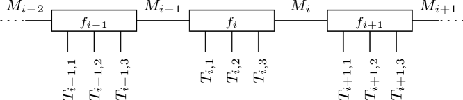
Figure 2: FFG for the convolutional stabilizer label codes in Exs. 10 and 11.

Example 10

(Convolutional Stab. QECC [6, Example 1]) With the help of our FFG framework, the stabilizer label code of [6, Example 1] can be seen to be given by the FFG in Figure 2, where, using the notation from Definition 1, $\mu_{i}=1$ for all $i$. For all $i$, the local function $f_{i}$ is given by

$$f_{i}(m_{i-1},t_{i,1},t_{i,2},t_{i,3},m_{i}) \triangleq\big{[}(m_{i-1},t_{i,1},t_{i,2},t_{i,3},m_{i})\in\mathcal{C}_{i}\big{]}$$

with $\mathcal{C}_{i}$ such that $\mathcal{C}_{\mathbb{F}_{4},i}\triangleq\gamma_{\mathbb{Z}_{2}^{2}\to\mathbb{F}_{4}}(\mathcal{C}_{i})$ is a linear code that is the $\mathbb{F}_{4}$-rowspan of the matrix

$$\left[\begin{array}[]{c|ccc|c}0&1&1&1&1\\ 1&1&\omega&\overline{\omega}&0\end{array}\right]\;.$$

(In order to obtain a block code one needs to terminate the FFG in Figure 2 on both sides; we omit the discussion of this issue. Alternatively, tail-biting can be used.) $\square$

Example 11

(Convolutional Stab. QECC [6, Example 3]) Similarly, we can represent the stabilizer label code of [6, Example 3] by the FFG in Figure 2. Here, however, we have $\mu_{i}=2$ for all $i$, and $\mathcal{C}_{i}$ is such that $\mathcal{C}_{\mathbb{F}_{4},i}\triangleq\gamma_{\mathbb{Z}_{2}^{2}\to\mathbb{F}_{4}}(\mathcal{C}_{i})$ is a linear code given by the $\mathbb{F}_{4}$-rowspan of

$$\left[\begin{array}[]{cc|ccc|cc}0&0&1&1&1&0&1\\ 0&1&1&0&0&1&1\\ 1&1&1&1&0&0&0\end{array}\right]\;.$$

Note that a “more common” choice for a matrix whose $\mathbb{F}_{4}$-rowspan is the trellis section code of a non-recursive convolutional code would have been a matrix like

$$\left[\begin{array}[]{cc|ccc|cc}0&0&1&1&1&0&1\\ 0&1&1&0&0&1&0\\ 1&0&1&1&0&0&0\end{array}\right]\;.$$

Here the rows are such that the last $\mu_{i}{-}1$ components of $m_{i-1}$ equal the first $\mu_{i}{-}1$ components of $m_{i}$. However, the $\mathbb{F}_{4}$-span of such a matrix does not result in a self-orthogonal $\mathcal{C}_{i}$. $\square$

Example 12

(Serial Turbo Stab. QECC [7, Figure 10]) The paper [7] discusses constructions of serial turbo stabilizer label codes. In particular, Figure 10 in [7] presents a code that corresponds to the FFG shown in Figure 3 (left). Here, $f_{\mathrm{convcode}1}$, $f_{\mathrm{quantum-interleaver}}$, and $f_{\mathrm{convcode}2}$ represent, respectively, the indicator functions of the first convolutional code, of the quantum interleaver, and of the second convolutional code. If the indicator functions correspond to self-orthogonal codes then we can apply our FFG framework and guarantee that the overall code is self-orthogonal. This is indeed the case for the codes presented in [7].

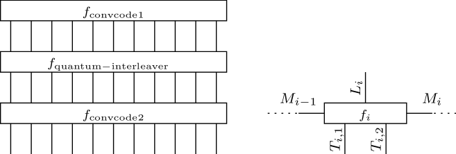
Figure 3: Left: FFG for the serial turbo stabilizer label code in Example 12. Right: FFG for the second convolutional code on the left-hand side.

A particular example of a stabilizer label code that can be used for the function node $f_{\mathrm{convcode}2}$ is given in [7, Figures 8 and 9] and shown as an FFG in Figure 3 (right). (In contrast to [7, Figures 8 and 9], that uses the variable names $P_{i,1}$ and $P_{i,2}$, we are using the variable names $T_{i,1}$ and $T_{i,2}$, respectively.) Here, for all $i$ the indicator function $f_{i}$ corresponds to a code $\mathcal{C}_{i}$ that is the rowspan of

$$\left[\begin{array}[]{ccccc|ccccc}1&0&1&1&1&0&0&0&0&0\\ 0&1&0&1&1&0&0&0&0&0\\ 0&0&0&0&0&1&0&1&0&0\\ 0&0&0&0&0&0&1&1&1&0\\ 0&0&0&0&0&0&0&0&1&1\end{array}\right]\;,$$

where the columns correspond to $m_{X,i-1}$, $l_{X,i}$, $t_{X,i,1}$, $t_{X,i,2}$, $m_{X,i}$, $m_{Z,i-1}$, $l_{Z,i}$, $t_{Z,i,1}$, $t_{Z,i,2}$, $m_{Z,i}$, respectively. Note that $\mathcal{C}_{i}$ is self-dual under the symplectic inner product and that the corresponding $\mathbb{F}_{4}$-code $\mathcal{C}_{\mathbb{F}_{4},i}\triangleq\gamma_{\mathbb{Z}_{2}^{2}\to\mathbb{F}_{4}}(\mathcal{C}_{i})$ is additive but not linear. (It cannot be linear since the number of codewords is $32$, which is not a power of $4$.) $\square$

Example 13

(Stabilizer State [11, Example 1]) Roughly speaking, a stabilizer state corresponds to a stabilizer QECC whose stabilizer label code is self-dual, see [12, 13, 11, 14]. Let $\mathbf{A}$ be the $n\times n$ adjacency matrix of any graph with $n$ vertices and let $\mathcal{C}$ be the rowspan of $\bigl{[}\,\mathbb{1}_{n}\,\bigl{|}\,\mathbf{A}\,\bigr{.}\bigr{]}$, where the columns correspond to $t_{X,1},\ldots,t_{X,n}$, $t_{Z,1},\ldots,t_{Z,n}$, and where $\mathbb{1}_{n}$ is the $n\times n$ identity matrix. It can easily be checked that $\mathcal{C}$ is self-dual under the symplectic inner product. (Note that $\mathbf{A}^{\mathrm{T}}=\mathbf{A}$ because $\mathbf{A}$ is the adjacency matrix of a graph.)

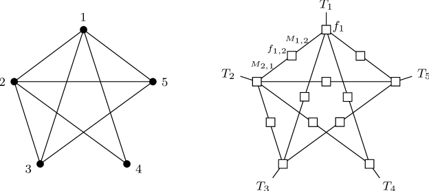
Figure 4: Left: graph with five vertices that defines a stabilizer state. Right: FFG of the corresponding stabilizer label code.

For example, the graph in Figure 4 (left) results in a stabilizer label code $\mathcal{C}$ which is the rowspan of

$$\left[\begin{array}[]{ccccc|ccccc}1&0&0&0&0&0&1&1&1&1\\ 0&1&0&0&0&1&0&1&1&1\\ 0&0&1&0&0&1&1&0&0&1\\ 0&0&0&1&0&1&1&0&0&0\\ 0&0&0&0&1&1&1&1&0&0\end{array}\right]\;.$$

It turns out that any such stabilizer label code can also be represented by an FFG that is topographically closely related to the graph that defined the code. E.g., Figure 4 (right) shows the FFG that corresponds to the example graph in Figure 4 (left). Here, $f_{1}$ is the indicator function of the self-dual code $\mathcal{C}_{1}$ which is defined to be the rowspan of

$$\left[\begin{array}[]{ccccc|ccccc}1&0&0&0&0&0&1&1&1&1\\ 0&1&0&0&0&1&0&0&0&0\\ 0&0&1&0&0&1&0&0&0&0\\ 0&0&0&1&0&1&0&0&0&0\\ 0&0&0&0&1&1&0&0&0&0\end{array}\right]\;,$$

where the columns correspond to $t_{X,1}$, $m_{X,1,2}$, $m_{X,1,3}$, $m_{X,1,4}$, $m_{X,1,5}$, $t_{Z,1}$, $m_{Z,1,2}$, $m_{Z,1,3}$, $m_{Z,1,4}$, $m_{Z,1,5}$, respectively. Moreover, $f_{1,2}$ is the indicator function of the self-dual code $\mathcal{C}_{1,2}$ which is defined to be the rowspan of $\left[\begin{array}[]{cc|cc}1&0&0&1\\ 0&1&1&0\end{array}\right]$, where the columns correspond to $m_{X,1,2}$, $m_{X,2,1}$, $m_{Z,1,2}$, $m_{Z,2,1}$, respectively. The other indicator functions $f_{i}$ and $f_{i,j}$ and self-dual codes $\mathcal{C}_{i}$ and $\mathcal{C}_{i,j}$ are defined analogously. Note that the code $\mathcal{C}_{i}$ depends on the number of vertices that are adjacent to vertex $i$. However, the code $\mathcal{C}_{i,j}$ is always the same for any pair $(i,j)$ of adjacent vertices. $\square$

Example 14

(LDPC codes) Any LDPC code whose parity-check matrix contains orthogonal rows can be used to construct a normalizer label code $\mathcal{C}^{\perp}$, see e.g. [5, 15, 16] and references therein. In terms of FFGs, such LDPC codes are expressed with the help of equal and single-parity-check function nodes. The FFG of the corresponding stabilizer label code $\mathcal{C}$ can also be expressed in terms of equal and single-parity-check function nodes. Because single-parity-checks of length not equal to $2$ do not represent self-orthogonal codes, our FFG framework is not directly applicable to construct FFGs of such LDPC codes. However, with the help of some auxiliary code constructions, our framework can also be used to construct LDPC stabilizer/normalizer label codes; because of space constraints we do not give the details here. $\square$

We leave it as an open problem to use our FFG framework to construct other classes of stabilizer label codes that have interesting properties.

VI Message-Passing Iterative and
Linear Programming Decoding

One of the main interests in studying FFGs for stabilizer label codes and their duals is that one would like to have FFGs that are suitable for MPI decoding. (Note that the code that is relevant for decoding in the stabilizer QECC framework is the code $\mathcal{C}^{\perp}$, or the coset code $\mathcal{C}^{\perp}/\mathcal{C}$, see e.g. the comments in [7].) The well-known trade-offs from classical LDPC and turbo codes apply also here: good codes with low FFG variable and function node complexity must have cycles, yet cycles lead to sub-optimal performance of message-passing iterative decoders. We leave it as an open problem to study stopping sets, trapping sets, absorbing sets, near-codewords, pseudo-codewords, the fundamental polytope, etc. (see e.g. the refs. at [17]) for the codes that were discussed in this paper. Moreover, one can formulate alternative decoders to MPI decoders like linear programming (LP) decoding. It would be interesting to see if the self-orthogonality property of stabilizer label codes leads to further insights in the context of MPI and LP decoders, in particular by also leveraging other duality results for FFGs like Fourier duality [18] and Lagrange duality [19].

References

• [1] F. R. Kschischang, B. J. Frey, and H.-A. Loeliger, “Factor graphs and the sum-product algorithm,” IEEE Trans. on Inform. Theory, vol. IT–47, no. 2, pp. 498–519, Feb. 2001.
• [2] M. A. Nielsen and I. L. Chuang, Quantum Computation and Quantum Information.   Cambridge, UK: Cambridge University Press, 2000.
• [3] D. Gottesman, “Stabilizer codes and quantum error correction,” Ph.D. dissertation, California Institute of Technology, Pasadena, CA, USA, 1997.
• [4] A. R. Calderbank, E. M. Rains, P. W. Shor, and N. J. A. Sloane, “Quantum error correction via codes over GF(4),” IEEE Trans. on Inform. Theory, vol. IT–44, no. 4, pp. 1369–1387, July 1998.
• [5] D. J. C. MacKay, G. Mitchison, and P. L. McFadden, “Sparse-graph codes for quantum error correction,” IEEE Trans. on Inform. Theory, vol. IT–50, no. 10, pp. 2315–2330, Oct. 2004.
• [6] G. D. Forney, Jr., M. Grassl, and S. Guha, “Convolutional and tail-biting quantum error-correcting codes,” IEEE Trans. on Inform. Theory, vol. IT–53, no. 3, pp. 865–880, Mar. 2007.
• [7] D. Poulin, J.-P. Tillich, and H. Ollivier, “Quantum serial turbo-codes,” submitted, available online under http://arxiv.org/abs/0712.2888, Dec. 2007.
• [8] G. D. Forney, Jr., “Codes on graphs: normal realizations,” IEEE Trans. on Inform. Theory, vol. IT–47, no. 2, pp. 520–548, Feb. 2001.
• [9] H.-A. Loeliger, “An introduction to factor graphs,” IEEE Sig. Proc. Mag., vol. 21, no. 1, pp. 28–41, Jan. 2004.
• [10] H. Wang, J. Wang, Q. Du, and G. Zeng, “A new approach to constructing CSS codes based on factor graphs,” Information Sciences, vol. 178, no. 7, pp. 1893–1902, Apr. 2008.
• [11] M. Van den Nest, J. Dehaene, and B. De Moor, “Graphical description of the action of local Clifford transformations on graph states,” Phys. Rev. A, vol. 69, no. 2, pp. 022 316.1–022 316.7, 2004.
• [12] D. Schlingemann and R. F. Werner, “Quantum error-correcting codes associated with graphs,” Phys. Rev. A, vol. 65, p. 012308, Dec. 2001.
• [13] D. Schlingemann, “Stabilizer codes can be realized as graph codes,” Quant. Inf. Comp., vol. 2, no. 4, pp. 307–323, June 2001.
• [14] A. Cross, G. Smith, J. A. Smolin, and B. Zeng, “Codeword stabilized quantum codes,” submitted, available online under http://arxiv.org/abs/0708.1021v1, Aug. 2007.
• [15] S. A. Aly, “A class of quantum LDPC codes constructed from finite geometries,” submitted, available online under http://aps.arxiv.org/abs/0712.4115, Dec. 2007.
• [16] I. Djordjevic, “Quantum LDPC codes from balanced incomplete block designs,” IEEE Comm. Letters, vol. 12, no. 5, pp. 389–391, May 2008.
• [17] http://www.pseudocodewords.info.
• [18] Y. Mao and F. R. Kschischang, “On factor graphs and the Fourier transform,” IEEE Trans. on Inform. Theory, vol. IT–51, no. 5, pp. 1635–1649, 2005.
• [19] P. O. Vontobel and H.-A. Loeliger, “On factor graphs and electrical networks,” in Mathematical Systems Theory in Biology, Communication, Computation, and Finance, IMA Volumes in Math. & Appl., D. Gilliam and J. Rosenthal, Eds.   Springer Verlag, 2003.