The Ups and Downs of Modeling Financial Time Series with Wiener Process Mixtures

Abstract

Starting from inhomogeneous time scaling and linear decorrelation between successive price returns, Baldovin and Stella recently proposed a way to build a model describing the time evolution of a financial index. We first make it fully explicit by using Student distributions instead of power law-truncated Lévy distributions; we also show that the analytic tractability of the model extends to the larger class of symmetric generalized hyperbolic distributions and provide a full computation of their multivariate characteristic functions; more generally, the stochastic processes arising in this framework are representable as mixtures of Wiener processes. The Baldovin and Stella model, while mimicking well volatility relaxation phenomena such as the Omori law, fails to reproduce other stylized facts such as the leverage effect or some time reversal asymmetries. We discuss how to modify the dynamics of this process in order to reproduce real data more accurately.

I How Scaling and Efficiency Constrains Return Distribution

Finding a faithful stochastic model of price time series is still an open problem. Not only should it replicate in a unified way all the empirical statistical regularities, often called stylized facts, (cf e.g. Cont (2001); Bouchaud and Potters (2003)), but it should also be easy to calibrate and analytically tractable, so as to facilitate its application to derivative pricing and financial risk assessment. Up to now none of the proposed models has been able to meet all these requirements despite their variety. Attempts include ARCH family (Bollerslev et al. (1994); Tsay (2002) and references therein), stochastic volatility (Musiela and Rutkowski (2005) and references therein), multifractal models (Borland et al. (2005); Eisler and Kertész (2004); Bacry et al. (2001a); Mandelbrot et al. (1997) and references therein), multi-timescale models (Borland and Bouchaud (2005); Zumbach (2004); Zumbach et al. (2000)), Lévy processes (Cont and Tankov (2004) and references therein), and self-similar processes (Carr et al. (2007)).

Recently Baldovin and Stella (B-S thereafter) proposed a new way of addressing the question. We advise the reader to refer to the original papers Baldovin and Stella (2007a, b, 2008) for a full description of the model as we shall only give a brief account of its main underlying principles. Using their notation let $S(t)$ be the value of the asset under consideration at time $t$, the logarithmic return over the interval $[t,t+\delta t]$ is given by $r_{t,\delta t}=\ln S(t+\delta t)-\ln S(t)$; the elementary time unit is a day, i.e., $t=0,1,\dots$ and $\delta t=1,2,\dots$days. In order to accommodate for non-stationary features, the distribution of $r_{t,\delta t}$ is denoted by $P_{t,\delta t}(r)$ which contains an explicit dependence on $t$. The most impressive achievement of B-S is to build the multivariate distribution $P_{0,1}^{(n)}(r_{0,1},\dots,r_{n,1})$ of $n$ consecutive daily returns starting from the univariate distribution of a single day provided that the following conditions hold:

1. No trivial arbitrage: the returns are linearly independent, i.e. $E(r_{i,1},r_{j,1})=0$ for $i\neq j$, with the standard condition $E(r_{i,1})=0$.

2. Possibly anomalous scaling of the return distribution with respect to the time interval $\delta t$, with exponent $D$:

   $$P_{0,\delta t}(r)=\frac{1}{\delta t^{D}}P_{0,1}\left(\frac{r}{\delta t^{D}}\right)\,.$$

3. Identical form of the unconditional distributions of the daily returns up to a possible dependence of the variance on the time $t$, i.e.

   $$P_{t,1}(r)=\frac{1}{a_{t}}P_{0,1}\left(\frac{r}{a_{t}}\right)\,.$$

As shown in the addendum of Baldovin and Stella (2007b) these conditions admit the solution

$$f_{0,1}^{(n)}(k_{1},\dots,k_{n})=\tilde{g}(\sqrt{a_{1}^{2D}k_{1}^{2}+\cdots+a_{n}^{2D}k_{n}^{2}}),$$ (1)

where $f_{0,1}^{(n)}$ is the characteristic function of $P_{0,1}^{(n)}$, $\tilde{g}$ the characteristic function of $P_{0,1}$, and $a_{i}^{2D}=i^{2D}-(i-1)^{2D}$. In this way the full process is entirely determined by the choice of the scaling exponent $D$ and the distribution $P_{0,1}$. Therefore the characteristic function of $P_{t,\delta t}(r)$ is

$$f_{t,T}(k)=f_{0,1}^{(n)}(\underbrace{0,\dots,0}_{t\textrm{ terms}},\underbrace{k,\dots,k}_{\delta t\textrm{ terms}},0,\dots,0)=\tilde{g}(k\sqrt{(t+\delta t)^{2D}-t^{2D}}),$$

i.e.

$$P_{t,\delta t}(r)=\frac{1}{\sqrt{(t+\delta t)^{2D}-t^{2D}}}P_{0,1}\left(\frac{r}{\sqrt{(t+\delta t)^{2D}-t^{2D}}}\right).$$

The functional form of $\tilde{g}$ in Eq. (1) introduces a dependence between the unconditional marginal distributions of the daily returns by the means of a generalized multiplication $\otimes$ in the space of characteristic functions, i.e.,

$$f_{0,1}^{(n)}(k_{1},\dots,k_{n})=\tilde{g}(a_{1}^{D}k_{1})\otimes_{\tilde{g}}\cdots\otimes_{\tilde{g}}\tilde{g}(a_{n}^{D}k_{n}),$$

with $\otimes_{\tilde{g}}$ defined by

$$x\otimes_{\tilde{g}}y=\tilde{g}\left(\sqrt{[\tilde{g}^{-1}(x)]^{2}+[\tilde{g}^{-1}(y)]^{2}}\right).$$ (2)

At first sight this last equation may seem a trivial identity, but it does hide a powerful statement. Suppose indeed that instead of starting with the probability distribution $\tilde{g}$, one takes a general distribution with finite variance $\sigma^{2}=2$ and characteristic function $\tilde{p}_{1}$, then it is shown in Baldovin and Stella (2007a) that

$$\lim_{N\rightarrow\infty}\underbrace{\tilde{p}_{1}\left(\frac{k}{\sqrt{N}}\right)\otimes_{\tilde{g}}\cdots\otimes_{\tilde{g}}\tilde{p}_{1}\left(\frac{k}{\sqrt{N}}\right)}_{N\textrm{ terms}}=\tilde{g}(k).$$ (3)

This means that in this framework the return distribution at large scales is independent of the distribution of the returns at microscopic scales: it is completely determined by the correlation introduced by the multiplication $\otimes_{\tilde{g}}$, with fixed point $\tilde{g}$. Note that if $\tilde{g}$ is the characteristic function of the Gaussian distribution, then $\otimes_{\tilde{g}}$ reduces to the standard multiplication and one recovers the standard Central Theorem Limit.

As the volatility of the model shrinks in an inexorable way, Baldovin and Stella propose to restart the whole shrinking process after a critical time $\tau_{c}$ long enough for the volatility autocorrelation to fall to the noise level. In this way one recovers a sort of stationary time series when their length is much greater than $\tau_{c}$. In this case one expects that the empirical distribution of the return $\bar{P}_{\delta t}(r)$ over a time horizon $\delta t\ll\tau_{c}$, evaluated with a sliding window satisfies

$$\bar{P}_{\delta t}(r)=\frac{1}{\tau_{c}}\sum_{t=0}^{\tau_{c}-1}P_{t,\delta t}(r).$$ (4)

In the original papers no market mechanism is proposed for modeling the restart of the process; it is simply stated that the length of different runs and the starting points of the processes could be stochastic variables. In their simulations the length of the processes was fixed to $\tau=500$, which corresponds to slightly more than two years of daily data.

II A Fully Explicit Theory with Student Distributions

In Baldovin and Stella (2007b) a power law truncated Lévy distribution is chosen to describe the returns

$$\tilde{g}(k)=\exp\left(\frac{-Bk^{2}}{1+C_{\alpha}k^{2-\alpha}}\right).$$ (5)

In Sokolov et al. (2004) it is shown that this expression is indeed the characteristic function of a probability density with power law tails whose exponent is exponent $5-\alpha$. However, this choice is problematic in two respects: its inverse Fourier cannot be computed explicitly, which prevents a fully explicit theory. In addition, for Eq. (1) to be consistent, $\tilde{g}(\sqrt{k_{1}^{2}+\cdots+k_{n}^{2}})$ must be the characteristic function of a multivariate probability density for all $n$. In Baldovin and Stella (2007b) only numerical checks are performed to verify this property. But as discussed for example in Bouchaud and Potters (2003) both truncated Lévy and Student distributions yield acceptable fits of the returns on medium and small time scales. In the present context, the Student distribution, sometimes referred to as $q$-Gaussian in the case of non-integer degrees of freedom, is a better choice; it provides analytic tractability while fitting equally well real stock market prices (see alsoOsorio et al. (2004)). The fit of the daily returns of the S&P 500 index in the period with a Student distribution

$$g_{1}(x)=\frac{\Gamma(\frac{\nu}{2}+\frac{1}{2})}{\pi^{1/2}\lambda\Gamma(\frac{\nu}{2})}\frac{1}{(1+\frac{x^{2}}{\lambda^{2}})^{\frac{\nu}{2}+\frac{1}{2}}}$$

is reported in Fig. 1.

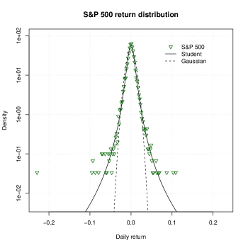
Figure 1: Centered distribution of the 14956 daily returns of the S&P 500 index (January, 3th 1950 - June, 11th 2009), and the corresponding fitting with Student ($\nu=3.21$, $\lambda=0.0109$) and Gaussian distribution ($\sigma=0.0095$).

The characteristic function of the Student density is

$$\tilde{g}(k)=\frac{2^{1-\frac{\nu}{2}}}{\Gamma(\frac{\nu}{2})}k^{\frac{\nu}{2}}K_{\frac{\nu}{2}}(k),$$ (6)

where $K_{\alpha}$ is the modified Bessel function of third kind. As demonstrated in the appendix, the inverse Fourier transform of $\tilde{g}(\sqrt{k_{1}^{2}+\cdots+k_{n}^{2}})$ for any integer $n$ is simply the multivariate Student distribution (see also Vignat and Plastino (2007)). The general form of this distribution can be written as

$$g_{n}^{(\nu)}(\mathbf{x},\mathbf{\Lambda})=\frac{\Gamma(\frac{\nu}{2}+\frac{n}{2})}{\pi^{n/2}(\det\mathbf{\Lambda})^{1/2}\Gamma(\frac{\nu}{2})}\frac{1}{(1+\mathbf{x}^{t}\mathbf{\Lambda}^{-1}\mathbf{x})^{\frac{\nu}{2}+\frac{n}{2}}}\,,$$ (7)

where $\nu>1$ is the exponent of the power law of the tails, $\mathcal{P}(r>R)\propto 1/R^{\nu}$ and $\mathbf{\Lambda}$ is a positive definite symmetric matrix governing the variance-covariance matrix $E(x_{i},x_{j})=\frac{\Lambda_{ij}}{\nu-2}$, which does exist provided that $\nu>2$.

In passing, the same properties are shared by multivariate symmetric generalized hyperbolic distributions introduced in finance by Eberlein and Keller (1995) (see also Bingham and Kiesel (2001a)). The general case is obtained by an affine change of variable, but for the sake of brevity let us restrict to

$$f(\mathbf{x})=\frac{\alpha^{\frac{n}{2}}}{(2\pi)^{\frac{n}{2}}K_{\frac{\nu}{2}}(\alpha)}\frac{1}{(1+r^{2})^{\frac{\nu}{4}+\frac{n}{4}}}K_{\frac{\nu}{2}+\frac{n}{2}}(\alpha\sqrt{1+r^{2}})$$

for $\mathbf{x}\in\mathbb{R}^{n}$ and $r$ the usual euclidean norm of $\mathbf{x}$. Student distributions are recovered in the limit $\alpha\rightarrow 0^{+}$. As shown in the appendix, its characteristic function is given for any $n$ by

$$\tilde{f}_{n}(\mathbf{k})=\frac{K_{\frac{\nu}{2}}(\sqrt{\alpha^{2}+k^{2}})}{K_{\frac{\nu}{2}}(\alpha)}\frac{(\alpha^{2}+k^{2})^{\frac{\nu}{4}}}{\alpha^{\frac{\nu}{2}}}$$

with $k=\sqrt{\sum_{i=1}^{n}k_{i}^{2}}$.

In the following we restrict the discussion to the Student distributions. Hence we assume that the distribution of the return is given by Eq. (7) with characteristic function given by Eq. (6), where $\mathbf{\Lambda}$ is a diagonal matrix

$$k=\sqrt{\mathbf{k}^{t}\mathbf{\Lambda}\mathbf{k}}=\lambda\sqrt{k_{0}^{2}+(2^{2D}-1)k_{1}^{2}+\cdots+(n^{2D}-(n-1)^{2D})k_{n-1}^{2}}$$

and $\lambda^{2}$ governs the variance of the returns on the time scale chosen as a reference. Thanks to the fact that the diagonal elements of $\mathbf{\Lambda}$ form a telescoping series the process is indeed consistent for any number of discrete steps. Moreover it can be generalized to the continuous time by setting, in the same consistent way,

$$\mathcal{P}(r_{0,\Delta t_{0}},r_{t_{1},\Delta t_{1}},\dots,r_{t_{n-1},\Delta t_{n-1}})\\ =g_{n}^{(\nu)}(r_{0,\Delta t_{0}},r_{t_{1},\Delta t_{1}},\dots,r_{t_{n-1},\Delta t_{n-1}},\mathbf{\Lambda}=\operatorname{diag}(t_{1}^{2D},t_{2}^{2D}-t_{1}^{2D},\dots,t_{n}^{2D}-t_{n-1}^{2D})),$$ (8)

where $t_{j}=\sum_{i=0}^{j-1}\Delta t_{i}$, $j\geq 1$ and now $\mathbf{\Lambda}=\operatorname{diag}(t_{1}^{2D},t_{2}^{2D}-t_{1}^{2D},\dots,t_{n}^{2D}-t_{n-1}^{2D})$. The existence of the continuum process is then guaranteed by the Kolmogorov extension theorem. Starting from this expression a wider class of processes can be generated by suitable transformations of the time, i.e., by substituting the function $t_{i}\rightarrow t_{i}^{2D}$ for any monotonically increasing continuous function $t_{i}\rightarrow T(t_{i})$. The process followed by the price $x(t)=\ln S(t)$ is a Student process too, with same exponent $\nu$ and non diagonal matrix $\Lambda_{ij}=(-1)^{i+j}T(t_{\min(i,j)})$.

The Student setting makes easier to interpret the correlations induced by the pointwise non-standard product of (2) in the characteristic function space. If we consider two variables $x_{1}$ and $x_{2}$ distributed according to $g_{1}(x)$, the joint probability function will be $g_{2}(x_{1},x_{2})$. The variables $X_{i}=G(x_{i})=\int_{-\infty}^{x_{i}}dx\,g_{1}(x)$ are distributed uniformly on the interval $[0,1]$; by definition, the copula function $c(X_{1},X_{2})$ (cf. e.g. Nelsen (2006) for a general theory) is

$$c(X_{1},X_{2})=g_{2}(G^{-1}(X_{1}),G^{-1}(X_{2}))\frac{dx_{1}}{dX_{1}}\frac{dx_{2}}{dX_{2}}=\frac{g_{2}(G^{-1}(X_{1}),G^{-1}(X_{2}))}{g(G^{-1}(X_{1}))\,g(G^{-1}(X_{2}))}.$$

In our case $c$ is none other than the Student copula function, generally applied in finance for describing the correlation among asset prices (Cherubini et al. (2004); Malevergne and Sornette (2006)). A picture of this copula density with $\nu=3$ and $\mathbf{\Lambda}$ the identity matrix is given in Fig. 2. Although Student and generalized hyperbolic distributions are usually adopted for modeling returns of several assets over the same time intervals, the framework proposed by Baldovin and Stella allow them to model the returns of a single asset over different time intervals.

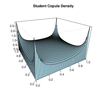
(a) 3D perspective.

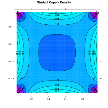
(b) Level plot.

Figure 2: Student copula density with $\nu=3$ and trivial correlation matrix.

III The Baldovin-Stella Process as Multivariate Normal Variance Mixtures

According to the B-S framework we have to look for functions $\phi:\,\mathbb{R}\rightarrow\mathbb{C}$, such that $\tilde{g}_{n}:\,\mathbb{R}^{n}\rightarrow\mathbb{C}$ with $\tilde{g}_{n}(k_{1},k_{2},\dots,k_{n})=\phi(k_{1}^{2}+k_{2}^{2}+\cdots+k_{n}^{2})$ is the characteristic function of a probability distribution for any $n$. Then from Eq. (8) we obtain a unique stochastic process with a well-defined continuous limit.

B-S processes can be fully characterized if one regards their finite dimensional marginals as instances of multivariate normal variance mixtures $U=\sigma N$, where $\sigma$ is an univariate random variable with positive values, $\sigma^{2}$ having cumulative distribution $G$, and $N$ is an $n$-dimensional normal random variable independent from $\sigma$. Leaving aside trivial affine changes of variables, we can assume that the covariance matrix of $N$ is the identity matrix. By first conditioning its evaluation on the value of $\sigma$, and then computing its mean over $\sigma$, it is immediate to see that the characteristic function $\tilde{g}_{n}^{U}(k_{1},k_{2},\dots,k_{n})$ of $U$ is

$$\tilde{g}_{n}^{U}(k_{1},k_{2},\dots,k_{n})=\phi_{\sigma^{2}}\left(\frac{1}{2}(k_{1}^{2}+k_{2}^{2}+\cdots+k_{n}^{2})\right),$$

where $\phi_{\sigma^{2}}(s)$ is the Laplace transform associated to $G$

$$\phi_{\sigma^{2}}(s)=\int_{0}^{\infty}dx\,e^{-sx}dG(x).$$

As this construction is independent from $n$, an admissible choice for $\phi$ is $\phi(s)=\phi_{\sigma^{2}}(\frac{s}{2})$, where $\phi_{\sigma^{2}}$ is the Laplace transform associated to any random variable $\sigma^{2}$ with positive values.

The crucial point is that by Schoenberg’s theorem in Schoenberg (1942) (see also the self-contained discussion about normal variance mixtures in Bingham and Kiesel (2001b)) this family exhausts all the possible choices, i.e. $\phi(k_{1}^{2}+k_{2}^{2}+\cdots+k_{n}^{2})$ is a characteristic function of a probability distribution for any $n$ if and only if $\phi(s)$ is the Laplace transform a univariate random variable with positive values.

Hence a multivariate distribution for the returns can be built in the B-S framework if and only if it admits a representation as a normal variance mixture.

In passing we note that the choice of B-S in their original papers for the distribution (5) is indeed admissible, as in Sokolov et al. (2004) it is shown that

$$\phi_{S}(s)=\exp\left(\frac{-Bs}{1+C_{\alpha}s^{1-\alpha/2}}\right)$$

is completely monotone, hence a Laplace transform by the virtue of Bernstein’s theorem.

Now it is immediate to see that all the stochastic processes $X_{t}^{\sigma}(\omega)$ that can arise in the B-S framework admit the following representation on a suitably chosen stochastic basis $(\Omega,\mathcal{F},\mathbb{P})$, over which a positive random variable $\sigma(\omega)$ and a Wiener process $W_{t}(\omega)$ independent from $\sigma$ are defined:

$$X_{t}^{\sigma}(\omega)=\sigma(\omega)W_{t^{2D}}(\omega)\,.$$ (9)

We only have to show that the finite dimensional marginal laws of $X_{t}^{\sigma}(\omega)$ are the same as those arising from (8). Indeed if we first evaluate the expectations over $W$, conditional on $\sigma$, we will obtain a Gaussian multivariate distribution

$$\mathcal{P}(X_{t_{1}},X_{t_{2}},\dots,X_{t_{n}}\mid\sigma)\\ =\frac{1}{(2\pi\sigma^{2})^{\frac{n}{2}}}\exp\left[-\frac{1}{2\sigma^{2}}\left(\frac{X_{t_{1}}^{2}}{t_{1}^{2D}}+\frac{(X_{t_{2}}-X_{t_{1}})^{2}}{t_{2}^{2D}-t_{1}^{2D}}+\cdots+\frac{(X_{t_{n}}-X_{t_{n-1}})^{2}}{t_{n}^{2D}-t_{n-1}^{2D}}\right)\right];$$

the eventual average over $\sigma$ will then lead to the same multivariate normal variance mixtures as in (8), with the appropriate covariance matrix (just note that $\Delta t_{i}=t_{i+1}-t_{i}$, and $r_{i,\Delta t_{i}}=X_{t_{i+1}}-X_{t_{i}}$). In particular, the processes introduced in Sec. II correspond to an inverse Gamma distribution of $\sigma^{2}$ in the Student case, and a Generalized Inverse Gaussian distribution in the hyperbolic case.

The stochastic differential equation obeyed by (9) is

$$dX_{t}^{\sigma}(\omega)=\sigma(\omega)t^{D-\frac{1}{2}}dW_{t}\,,$$

This equation shows that the volatility of the processes admissible in the B-S framework has a deterministic time dynamic, and that its source of randomness is just ascribable to its initial value.

Eventually we can conclude that a stochastic process is compatible with the B-S framework if and only if it is a variance mixture of Wiener processes whose variance is distributed according an arbitrary positive law, with a deterministic power law time change. This explains why using use this framework to model real price returns, one inevitably has to assume that the real price dynamics is composed by sequences of different realizations, as done by B-S. This is necessary not only because otherwise the model would predict a persistent and deterministic volatility decay for $D<1/2$, but also because $\sigma$ is fixed in each realization. The limitations of this kind of models in describing real returns will be made more manifest in the following section, but now we already know their mathematical foundations.

The asset prices can be modeled in an obvious arbitrage free way

$$S(t,\omega)=S_{0}\exp\left(rt+\sigma(\omega)W_{t^{2D}}(\omega)-\frac{1}{2}\sigma^{2}(\omega)t^{2D}\right)\,,$$

with $r$ the fixed default free interest rate, and where we left the dependence on $\omega$ explicit in order to emphasise the fact that $\sigma$ is a random variable. The pricing of options is then the same as in the Black-Scholes model, with an additional average over $\sigma(\omega)$. For instance the price $C(T,K)$ of a call option with maturity $T$ and strike $K$ is

$$C(T,K)=S_{0}E_{\sigma}(N(d_{1}))-e^{-rT}KE_{\sigma}(N(d_{2}))\,,$$

with as usual $N$ is the normal cumulative distribution,

$$d_{1}= \frac{\ln\frac{S_{0}}{K}+rt+\frac{1}{2}\sigma^{2}t^{2D}}{\sigma t^{D}}\,,$$

$$d_{2}= \frac{\ln\frac{S_{0}}{K}+rt-\frac{1}{2}\sigma^{2}t^{2D}}{\sigma t^{D}}\,,$$

and the additional expectation $E_{\sigma}$ has to be evaluated according to the distribution of $\sigma.$

IV Applicability of this Framework to Real Markets

The axiomatic nature of the derivation of Baldovin and Stella is elegant and powerful: its ability to build mathematically multivariate price return distributions from a univariate distribution using only a few reasonable assumptions is impressive. Nevertheless, as stated in the introduction, a model of price dynamics must meet many requirements in order to be both relevant and useful. In this section, we examine its dynamics thoroughly.

IV.1 Volatility dynamics

In Fig. 3.a we report the results of three simulations of the return process, each one of 500 steps and with parameters $\nu=3.2$ and $D=0.20$. In each run the volatility decays ineluctably, as explained in the previous section. Indeed by fixing the time interval $\delta t_{i}=1$, we see from Eq. (8) that the unconditional volatility of the $r_{t,1}$ returns is proportional to $\sqrt{(t+1)^{2D}-t^{2D}}$, i.e., to $t^{D-1/2}$ for $t\gg 1$: the unconditional volatility decreases if $D<1/2$ and increases if $D>1/2$, in both cases according to a power law. This appears quite clearly in Fig. 3.b, where we have computed the mean volatility decay, measured as the absolute values of the return, over 10000 process simulations. The parameters of the distributions have been chosen close to those representing real returns (see below).

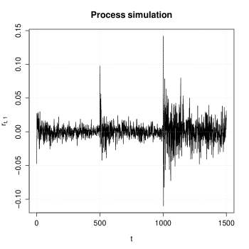
(a) Three simulations, each 500 steps long.

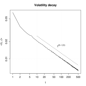
(b) Decay of the volatility: average over 10000 simulation, each 500 steps long. The dashed line represents the analytic prediction.

Figure 3: Process simulation with $\nu=3.2$, $D=0.20$, and $\lambda=0.107$.

The conditional volatility can be easily computed: the distribution of the return $r_{n,1}$ conditioned to the previous return realizations $r_{0,1},\dots,r_{n-1,1}$ is again a Student distribution with exponent $\nu\prime=\nu+n$ and conditional variance

$$[(n+1)^{2D}-n^{2D}]\left(1+\sum_{i=0}^{n-1}\frac{r_{i,1}^{2}}{(i+1)^{2D}-i^{2D}}\right).$$

From this expression it is clear that volatility spikes in a given realisation of the process tend to be persistent (see Fig. 3.a); this is the main reason why fluctuation patterns differ much from one run to an other. This can be also understood by appealing to the characterization of this kind of processes we did in Sec. III: each single run is just a realization of a Wiener process, whose variance is chosen at the beginning according to an Inverse Gamma distribution $R\Gamma(\frac{\nu}{2},\frac{\lambda}{2})$, and that decays in time according to the deterministic law $t^{D-\frac{1}{2}}$.

IV.2 Decreasing volatility and restarts

The very first model introduced by B-S has constant volatility, which corresponds to $\mathbf{\Lambda}$ being a multiple of the identity matrix. This unfortunate feature is the main reason behind the introduction of weights, whose effect is akin to an algebraic stretching of the time, or, as put forward by B-S, to a time renormalization. This in turn causes a deterministic algebraic decrease of the expectation of the volatility, as explained above and depicted in Fig. 3.b; hence the need for restarts, each attributed to an external cause.

Although this dynamics may seem quite peculiar, such restarts are found at market crashes, like the recent one of October 2008, which are followed by periods of algebraically decaying volatility. This leads to an analogous of the Omori law for earthquakes, as reported in Lillo and Mantegna (2003) and Weber et al. (2007). The B-S model, by construction, is able to reproduce this effect in a faithfully way. In Fig. 4 the cumulative number of times the absolute value of the returns $N(t)$ exceeds a given thresholds is depicted, for a single simulation of the process and three different value of the threshold. The fit with the prediction of the Omori law $N(t)=K(t+t_{0})^{\alpha}-Kt_{0}^{\alpha}$ is evident.

Crashes are good restart candidates: they provide clearly defined events that synchronize all the traders’ actions. In that view, they provide an other indirect way to measure the distribution of timescales of traders, which are thought to be power-law distributed (Lillo (2007)).

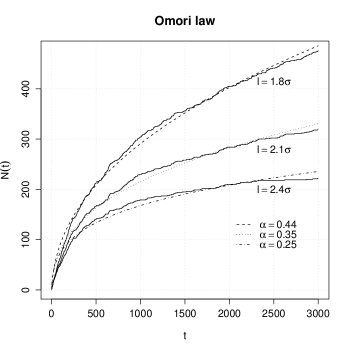
Figure 4: Omori law for a single run of the process, with $D=0.20$, $\nu=0.32$. $N(t)$ is the cumulative number the absolute value of the return exceeds a given thresholds. Three different values of the threshold $l$ have been chosen, measured with respect to the standard deviation $\sigma$ of the data. The dashed lines represents the fit with the Omori law $N(t)=K(t+t_{0})^{\alpha}-Kt_{0}^{\alpha}$.

Another example of algebraically decreasing volatility was recently reported by McCauley et al. (2007) in foreign exchange markets in which trading is performed around the clock. Understandably, when a given market zone (Asia, Europe, America) opens, an increase of activity is seen, and vice-versa. Specifically, this work fits the decrease of activity corresponding to the afternoon trading session in the USA with a power-law and finds an algebraic decay with exponent $\eta=0.35$; this is exactly the same behavior as the one of B-S model between two restarts, with $D=1-2\eta=0.3$. No explanation of why the trading activity should result in this specific type of decay has been put forward in our knowledge. In this case the starting time of the volatility decay corresponds to the maximum of activity of US markets.

IV.3 Apparent multifractality

The Baldovin and Stella model is able to reproduce the apparent multifractal characteristics of the real returns, i.e. the shape of $\zeta(q)$ where $\langle|r_{\delta t}|^{q}\rangle=\delta t^{\zeta(q)}$.

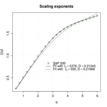
(a) Fitting of the empirical exponents of real data.

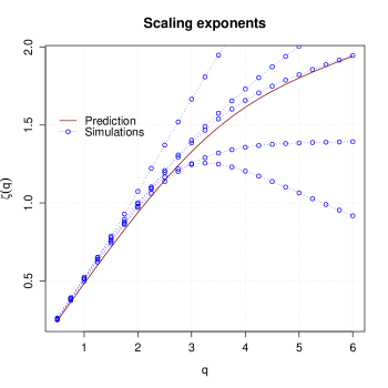
(b) Theoretical prediction compared to 5 simulations done with the same parameters.

Figure 5: Scaling exponents: S&P 500 data and simulations compared with theoretical prediction. All the simulations have been done with the same parameters: 30 runs of 500 steps, with $\nu=3.2$, $D=0.220$

The expectation is evaluated according the distribution (4), i.e. taking the mean over independent runs of the process. Hence the expectation of the $q$th moment in this model is

$$\langle|r|^{q}\rangle_{\bar{P}_{\delta t}}=\frac{\langle|r|^{q}\rangle_{P_{t=0,\delta t=1}}}{\tau_{c}}\sum_{t=0}^{\tau_{c}-1}[(t+\delta t)^{2D}-t^{2D}]^{q/2}$$ (10)

(see the addendum to Baldovin and Stella (2007b)). The exponents $\zeta(q)$ are evaluated as the slopes of the linear fitting of $\ln(\langle|r|^{q}\rangle_{\bar{P}_{\delta t}})$ with respect to $\ln(\delta t)$. Hence in our case they are determined by the expression $\ln\sum_{t=0}^{\tau_{c}-1}[(t+\delta t)^{2D}-t^{2D}]^{q/2}$, and depend only on $D$ and $\tau_{c}$. In Fig. 5.a is depicted the fitting of the S&P 500 exponents with the model (10). The best fit is obtained with $D=0.212$ and $\tau_{c}=5376$. Unfortunately a value of $\tau_{c}$ that large is difficult to justify, as in the case of S&P 500 we have only 14956 daily returns, i.e. less than three runs of a process with such a length. The other fit is obtained by first fixing $\tau_{c}=500$, as in Baldovin and Stella (2007b) and yields $D=0.220$.

The statistical significance of this approach seems anyway questionable. In Fig. 5.b we compare the theoretical expectation of the exponents with simulations. We choose the parameters $\tau_{c}=500$, $D=0.220$ both for simulations and analytic model, with $\nu=3.22$. The number of restarts in the simulation is 30 in order to have a number of data points similar to the S&P 500. It is evident that the exponents evaluated from the simulated data have a really large variance.

The problem is that if the tail exponent $\nu=3.22$, from an analytic perspective the moments with $q>3.22$ are infinite, hence, should not be taken into account in the multifractal analysis (for an analytic treatment of multifractal analysis see Riedi (2002); Jaffard (1997a, b)). The situation is somehow different in the case of multifractal models of asset returns (Bacry et al. (2001b); Mandelbrot et al. (1997)), where the theoretical prediction of the tail exponents of the return distribution is relatively high (see the review of Borland et al. (2005)), and the moments usually empirically measured do exist even from the analytic point of view. For attempts to reconcile the theoretical predictions of the multifractal models with real data see Bacry et al. (2006) and Muzy et al. (2006).

It is worth remembering that the anomalous scaling of the empirical return moments does not imply that the return series has to be described by a multifractal model, as already pointed out some time ago in Bouchaud (1999) and Bouchaud et al. (2000): the long memory of the volatility is responsible at least in part for the deviation from trivial scaling. A more detailed analysis of real data reported in Jiang and Zhou (2008) seems indeed to exclude evident multifractal properties of the price series.

V Missing Features

Since in this model the volatility is constant in each realization and bound to decrease unless a restart occurs, it is quite clear that it does not contain all the richness of financial market price dynamics. Restarting the whole process is not entirely satisfactory, as in reality the increase of volatility is not always due to an external shock. Volatility does often gradually build up through a feedback loop that is absent from the B-S mechanism. Thus, large events and crashes can also have a endogenous cause, e.g. due to the influence of traders that base their decisions on previous prices or volatility, such as technical analysts or hedgers. A quantitative description of this kind of phenomena is attempted for instance in Sornette (2003); Sornette et al. (2003), by appealing to discrete scale invariance (see also the viewpoint expressed in Chang and Feigenbaum (2006) and references therein). This kind of effect is completely missing from the original B-S mechanism.

Volatility build-ups can be simulated with $D>1/2$, getting at constant $D$ the equivalent of the inverse Omori law for earthquakes (Helmstetter et al., 2003). This kind of dynamics has been reported to happen prior to some financial market crashes (Sornette et al., 2003). At a smaller time scale, foreign exchange intraday volatility patterns have a systematically increasing part whose fit to a possibly arbitrary power-law, as performed in McCauley et al. (2007) ($\eta=0.22$), corresponds indeed to choosing $D=0.56$. To our knowledge, volatility build-ups either do not follow a particular and systematic law, or perhaps have not yet been the objects of a thorough study.

Because of the symmetric nature of all the distributions derived above, all the odd moments are zero, hence, the skewness of real prices cannot be reproduced. This shows up well in Fig. 3 of Baldovin and Stella (2008). Another consequence is that it is impossible to replicate the leverage effect, i.e. the negative correlation between past returns and future volatility, carefully analyzed in Bouchaud et al. (2001).

In any case, the decrease of the fluctuations in the B-S process is a deterministic outcome of the anomalous scaling law $t^{D}$ with $D<1/2$, and results in a strong temporal asymmetry of the corresponding time series. But quite remarkably it misses the time-reversal asymmetry reported in Lynch and Zumbach (2003) and Zumbach (2007). Indeed real financial time series are not symmetric under time reversal with respect to even-order moments. For instance, there is no leverage effect in foreign exchange rates, and their time series are not as skewed as indices, but they do have a time arrow. One of the indicators proposed in Lynch and Zumbach (2003) is the correlation between historical volatility $\sigma_{\delta t_{h}}^{(h)}(t)$ and realized volatility $\sigma_{\delta t_{r}}^{(r)}(t)$. The historical volatility series $\sigma_{\delta t_{h}}^{(h)}(t)$ represents the volatility computed using the data in the past interval $[t-\delta t_{h},t]$, and $\sigma_{\delta t_{r}}^{(r)}(t)$ represents the volatility computed using the data in the future interval $[t,t+\delta t_{r}]$; the correlation between the two series is then analyzed as a function of both $\delta t_{r}$ and $\delta t_{h}$. Real financial time series present an asymmetric graph with respect the change $\delta t_{h}\leftrightarrow\delta t_{s}$, with a strong indication that historical volatility at a given time scale $\delta t_{h}$ is more likely correlated to realized volatility with time scale $\delta t_{r}<\delta t_{h}$, with peaks of correlation at time scales related to human activities. The asymmetry characteristic is absent in the Baldovin and Stella model, as showed in Fig. 6.

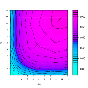
(a)

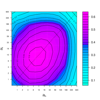
(b)

Figure 6: Correlation between historical and realized volatility of the simulated process, over different time interval $\delta t$. The analyzed time series was composed by 1000 runs of the basic process, each one with 200 steps, and parameter $\nu=3.22$, $D=0.20$.

The strong correlation between returns guarantees the slow decay of the volatility but induces some side effects. The distribution of the returns in the model is essentially the same with identical power law exponent for the tails. This happens independently of the time interval $\delta t$ over which the returns are evaluated, as long as $\delta t\ll\tau_{c}$, with $\tau_{c}$ of the order of hundreds days. Hence the weekly returns are distributed as the daily returns, while in real data the tail exponent begins to increase in a remarkable way already at the intraday level (Drozdz et al. (2007)). The strong correlation also slows down the convergence to the Gaussian distribution of the returns when measured on larger time scale. Even if the kurtosis is not defined analytically in principle, it is possible to measure the empirical kurtosis of the returns of a simulated time series and compare with the kurtosis of real data. In Fig. 7 we show the kurtosis of the return distribution among simulations and daily return of the S&P 500 index; the kurtosis has been computed for the returns over different interval $\delta t$, and the simulated processes had the same length (30 runs of 500 steps) of the real series.

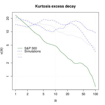
Figure 7: Comparison of the kurtosis of the returns evaluated over a time interval $\delta t$. Each one of the three simulations are composed by 30 runs, 500 steps long, in order to have a length comparable with that of the S&P 500 returns. The parameters are $\nu=3.2$, $D=0.20$, $\lambda=0.1$.

VI Suggested Improvements

The main limitations of the model proposed by Baldovin and Stella are poor volatility dynamics, lack of skewness, some unwanted symmetry with respect to time, and extremely slow convergence to a Gaussian. In this final section we put forward briefly some qualitative proposals of how these issues can be addressed.

The volatility dynamics can be improved by introducing an appropriate dynamics for the exponent $D$, i.e. introducing a dynamic $D(t)$ controlling the diffusive process. This is equivalent to starting with a model with constant volatility, i.e. with $\mathbf{\Lambda}$ proportional to the identity matrix, and then introducing an appropriate evolution for the time $t$. This technique is employed for instance in the Multifractal Random Walk model (Bacry et al. (2001b)), where the time evolution is driven by a multifractal process, or when the time evolution is modeled by an increasing Lévy process (see e.g. Cont and Tankov (2004)). In this last case we would obtain a mixing of Wiener processes driven by a subordinator.

The lack of skewness is a common problem of stochastic volatility models: one usually writes the return at time $t$ as $r_{t,\delta t}=\epsilon(t)\sigma(t)$, where $\epsilon(t)$ is sign of the return and $\sigma(t)$ its amplitude, a symmetric setting if the distribution of $\epsilon(t)$ is even. One remedy found for instance in Eisler and Kertész (2004) is to bias the sign probabilities while enforcing a zero expectation; more precisely,

$$P\left(\epsilon=\pm\frac{1/\sqrt{2}}{1/2\pm\epsilon}\right)=1/2\pm\epsilon.$$

Another possibility for introducing skewness is that of considering normal mean-variance mixtures, instead of simply normal variance ones. For instance, this would have implied the use of the multivariate skewed Student distribution in the model described in Sec. II.

The decay of the tail exponent of the return distribution, represented in Fig. 7, could be implemented by introducing two different Student distributions: a univariate with exponent $\nu_{r}$ for modeling the daily returns, and a multivariate one with a much larger exponent $\nu_{c}$ for modeling the correlations among them. By taking into account the generalized central limit theorem expressed in Eq. (3), the distribution of returns at intermediate time scales will interpolate between the two exponents, yielding the desired feature.

The Zumbach mugshot is one of the most difficult stylized facts to reproduce. To our knowledge the best results in that respect was achieved in Borland and Bouchaud (2005), where a specific realization of a quadratic GARCH model is introduced, motivated by the different activity levels of traders with different investment time horizons, which take into account the return over a large spectrum of time scales. More specifically Borland and Bouchaud use

$$\sigma_{i}^{2}=\sigma_{0}^{2}\left[1+\sum_{\delta t=1}^{\infty}\mathit{g_{\Delta t}}\frac{r_{i,\delta t}^{2}}{\sigma_{0}^{2}\tau\delta t}\right],$$

with $\tau$ fixing the time scale, $r_{t,\delta T}=\ln S(t+\delta T)-\ln S(t)$, $g_{\delta t}$ measuring the impact on the volatility by traders with time horizon $\delta t$, and chosen by the authors $g_{\delta t}=g/(\delta t)^{\alpha}$. This expression is rewritten also in the form

$$\sigma_{i}^{2}=\sigma_{0}^{2}+\sum_{j<i,k<i}\mathcal{M}(i,j,k)\frac{r_{j}r_{k}}{\tau},$$

with

$$\mathcal{M}(i,j,k)=\sum_{\Delta t=\max(i-j,i-k)}^{\infty}\frac{g_{\delta t}}{\delta t}.$$

In the present framework this would correspond to use a highly non-trivial matrix $\mathbf{\Lambda}$, introducing linear correlation among returns at any time lag. This means that the B-S process would no longer be a model of returns, but of stochastic volatility.

VII Discussion and Conclusions

When employed with self-decomposable distributions like the Student or the Generalized Hyperbolic as introduced in Sec. II, the resulting description of the process return is different than that of other models in the literature. First our Student process is not stationary, hence different from the class of Student processes discussed in Heyde and Leonenko (2005), where the main focus is on stationary ones. The processes (9) are also different from the one studied in Borland (2002): the latter too are continuous and based on the Student distributions, but defined by the stochastic differential equation

$$dX_{t}=t^{D-\frac{1}{2}}\sqrt{\frac{2Dc_{0}}{\nu-1}}\sqrt{1+\frac{X_{t}^{2}}{c_{0}t^{2D}}}dW\,;$$

apart from the striking difference with Eq. (9), in Vellekoop and Nieuwenhuis (2007) it is shown that not all the marginal distribution laws of $X_{t}$ are of Student type.

Instead in Eberlein and Keller (1995) the Generalized Hyperbolic laws are adopted for describing the returns at a fixed time scale; these laws are then extended to the other time scales using the standard Lévy process construction: in this case the distributions at the other time scales are no more of Generalized Hyperbolic type.

The Baldovin and Stella model is also intrinsically simpler than the ones described in Barndorff-Nielsen and Shephard (2001), where the volatility has a dynamic modeled by Ornstein-Uhlenbeck type processes,

$$d\sigma_{t}^{2}=-\lambda\sigma_{t}^{2}dt+dL_{t}$$

driven by an arbitrary Lévy process $L_{t}$. In this case, according to the choice of $L_{t}$, any self-decomposable distribution (like the Generalized Inverse Gaussian, or any of its special cases, like the Inverse Gamma) can arise as the distribution of $\sigma_{t}^{2}$ for any $t$. But this simplification comes at a high price: while in Barndorff-Nielsen $\sigma$ is truly dynamic, it is fixed in B-S for any single process realization.

In addition, the models analyzed in Carr et al. (2007) are of a different type, even if there are some analogies in the underlying principles. In Carr et al. (2007) indeed an anomalous scaling is introduced by considering self-similar processes, and in that framework any self-decomposable distribution can employed for modeling returns, but once again only at a fixed time scale, as in the standard case of Lévy processes. The main difference is that in Carr et al. (2007) the returns at different times are assumed to be totally independent, but not identically distributed: instead Baldovin and Stella assume that the returns are only linearly independent, but now with identical distributions at all the time scales, up to a simple rescaling.

In conclusion, despite its current inability to reproduce all the needed stylized facts, the new framework proposed by Baldovin and Stella introduces a new mechanism for modeling returns, based on a few reasonable first principles. We therefore think that, once suitably modified for instance along the lines proposed above, the B-S framework can provide a new tool for building models of financial price dynamics from reasonable assumptions.

Appendix: Some Useful Facts About Student and Symmetric Generalized Hyperbolic Distributions

Characteristic function of Student distributions

The standard form of univariate Student distribution is

$$g_{1}(x)=\frac{\Gamma(\frac{\nu}{2}+\frac{1}{2})}{\pi^{1/2}\Gamma(\frac{\nu}{2})}\frac{1}{(1+x^{2})^{\frac{\nu}{2}+\frac{1}{2}}},$$

while the multivariate one is

$$g_{n}(\mathbf{x})=\frac{\Gamma(\frac{\nu}{2}+\frac{n}{2})}{\pi^{n/2}\Gamma(\frac{\nu}{2})}\frac{1}{(1+r^{2})^{\frac{\nu}{2}+\frac{n}{2}}}$$

with $r=\sqrt{\sum_{i=1}^{n}x_{i}^{2}}$ and $\mathcal{P}(r>R)\propto 1/R^{v}$.

Using some standard relationships involving Bessel functions one can compute analytically the corresponding characteristic function:

$$\tilde{g}_{1}(k_{1})=\int_{-\infty}^{+\infty}dx_{1}\,e^{ik_{1}x_{1}}g_{1}(x_{1})\\ =\frac{2\Gamma(\frac{\nu}{2}+\frac{1}{2})}{\pi^{1/2}\Gamma(\frac{\nu}{2})}k^{\nu}\int_{0}^{+\infty}dx\,(k^{2}+x^{2})^{-\frac{\nu}{2}-\frac{1}{2}}\cos(x)=\frac{2^{1-\frac{\nu}{2}}}{\Gamma(\frac{\nu}{2})}k^{\frac{\nu}{2}}K_{\frac{\nu}{2}}(k),$$

with $k=|k_{1}|$, $K_{\alpha}$ the modified Bessel function of third kind, and the employ of identity 7.12.(27) of Erdélyi (1953)

$$K_{\nu}(z)=\frac{(2z)^{\nu}}{\pi^{1/2}}\Gamma(\nu+\frac{1}{2})\int_{0}^{\infty}dt\,(t^{2}+z^{2})^{-\nu-1/2}\cos(t)\\ \Re(\nu)>-\frac{1}{2},\;\mid\arg(z)\mid<\frac{\pi}{2}.$$

For an alternative derivation we refer to Hurst (1995) and to the discussion in Heyde and Leonenko (2005). An alternative expression is found in Dreier and Kotz (2002).

For general $n$ we obtain again the same expression. Indeed

$$\tilde{g}_{n}(\mathbf{k})=\int_{\mathbb{R}^{n}}d^{n}\mathbf{x}\,e^{i\mathbf{k}\cdot\mathbf{x}}g_{n}(\mathbf{x})\\ =\frac{\Gamma(\frac{\nu}{2}+\frac{n}{2})}{\pi^{n/2}\Gamma(\frac{\nu}{2})}\int d^{n-2}\Omega\int_{0}^{+\infty}dr\,r^{n-1}\int_{0}^{\pi}d\phi\,\sin^{n-2}(\phi)e^{ikr\cos\phi}(1+r^{2})^{-\frac{\nu}{2}-\frac{n}{2}}\\ =\frac{2^{n/2}\Gamma(\frac{\nu+n}{2})}{\Gamma(\frac{\nu}{2})}k^{1-n/2}\int_{0}^{+\infty}dr\,r^{n/2}(1+r^{2})^{-\frac{\nu}{2}-\frac{n}{2}}J_{n/2-1}(kr)\\ =\frac{2^{1-\frac{\nu}{2}}}{\Gamma(\frac{\nu}{2})}k^{\frac{\nu}{2}}K_{\frac{\nu}{2}}(k),$$

with $k=\sqrt{\sum_{i=1}^{n}k_{i}^{2}}$, $d^{n-2}\Omega$ the surface element of the sphere $S^{n-2}$, $\phi$ the angle between $\mathbf{k}$ and $\mathbf{x}$ and the employ of identities 7.12.(9)

$$\Gamma(\nu+\frac{1}{2})J_{\nu}(z)=\frac{1}{\pi^{1/2}}(\frac{z}{2})^{\nu}\int_{0}^{\pi}d\phi\,e^{iz\cos\phi}(\sin\phi)^{2\nu}\\ \Re(\nu)>-\frac{1}{2}\,,$$ (11)

and 7.14.(51) of Erdélyi (1953),

$$\int_{0}^{\infty}dt\,J_{\mu}(bt)(t^{2}+z^{2})^{-\nu}t^{\mu+1}=(\frac{b}{2})^{\nu-1}\frac{z^{1+\mu-\nu}}{\Gamma(\nu)}K_{\nu-\mu-1}(bz)\\ \Re(2\nu-\frac{1}{2})>\Re(\mu)>-1,\;\Re(z)>0.$$

Eventually one finds

$$\tilde{g}_{n}(\mathbf{k})=\tilde{g}_{1}\left(\sqrt{k_{1}^{2}+\cdots+k_{2}^{2}}\right).$$

With the linear change of variables $\mathbf{x}\rightarrow\mathbf{C}^{-1}\mathbf{x}$, setting $\mathbf{\Lambda}^{-1}=(\mathbf{C}^{T})^{-1}\mathbf{C}^{-1}$, i.e. $\mathbf{\Lambda}=\mathbf{C}\mathbf{C}^{T}$, one obtains the following generalizations:

$$g_{n}(\mathbf{x})=\frac{\Gamma(\frac{\nu}{2}+\frac{n}{2})}{\pi^{n/2}(\det\mathbf{\Lambda})^{1/2}\Gamma(\frac{\nu}{2})}\frac{1}{(1+\mathbf{x}^{t}\mathbf{\Lambda}^{-1}\mathbf{x})^{\frac{\nu}{2}+\frac{n}{2}}}\,,$$ (12)

with characteristic function

$$\tilde{g_{n}}(\mathbf{k})=\frac{2^{1-\frac{\nu}{2}}}{\Gamma(\frac{\nu}{2})}(\mathbf{k}^{t}\mathbf{\Lambda}\mathbf{k})^{\frac{\nu}{4}}K_{\frac{\nu}{2}}((\mathbf{k}^{t}\mathbf{\Lambda}\mathbf{k})^{1/2}).$$

In the univariate case $\mathbf{\Lambda}$ is substituted by the scalar $\lambda^{2}$ and the previous expressions reduce to

$$g_{1}(x)=\frac{\Gamma(\frac{\nu}{2}+\frac{1}{2})}{\pi^{1/2}\lambda\Gamma(\frac{\nu}{2})}\frac{1}{(1+\frac{x^{2}}{\lambda^{2}})^{\frac{\nu}{2}+\frac{1}{2}}}$$ (13)

and

$$\tilde{g}_{1}(k)=\frac{2^{1-\frac{\nu}{2}}}{\Gamma(\frac{\nu}{2})}(\lambda k)^{\frac{\nu}{2}}K_{\frac{\nu}{2}}(\lambda k).$$

Moments of Student distributions

Due to the symmetry under reflection all the odd moments vanish. For the second moments we have, provided that $\nu>2$,

$$E(x_{i},x_{j})=\frac{\Lambda_{ij}}{\nu-2}\,.$$

The moments of order $2n$ exist provided that $\nu>2n$ ; as happens for Gaussian distributions, they can be expressed in term of the second moments,

$$E(x_{j_{1}},x_{j_{2}},\dots,x_{j_{2n}}) = \frac{\Gamma(\frac{\nu}{2}-n)}{2^{n}\Gamma(\frac{\nu}{2})}\prod_{\textrm{all the pairings}}\Lambda_{j_{i_{1}}j_{i_{2}}}\cdots\Lambda_{j_{i_{2n-1}}j_{i_{2n}}}.$$

In the univariate case these formulas reduce to $E(x^{2})=\frac{\lambda^{2}}{\nu-2}$ and

$$E(x^{2n})=\frac{(2n-1)!!\Gamma(\frac{\nu}{2}-n)}{2^{n}\Gamma(\frac{\nu}{2})}\lambda^{2n}.$$

The kurtosis is then $\kappa=3\frac{\nu-2}{\nu-4}$, provided that $\nu>4$.

Simulation of multivariate Student distributions

The simulation is a standard application of the technique used in the case of rotational invariance. From

$$g_{n}(\mathbf{x})d^{n}\mathbf{x}=\frac{\Gamma(\frac{\nu}{2}+\frac{n}{2})}{\pi^{n/2}\Gamma(\frac{\nu}{2})}r^{n-1}(1+r^{2})^{\frac{1}{1-q}}d^{n-1}\Omega dr,$$

with $r\geq 0$, we see that the density of the angular variables is uniform, while setting $y=\frac{r^{2}}{1+r^{2}}$, with $1>y\geq 0$ and $r=\sqrt{y/(1-y)}$, the density of $y$ is given by

$$\frac{1}{B(\frac{n}{2},\frac{\nu}{2})}y^{\frac{n}{2}-1}(1-y)^{\frac{\nu}{2}-1}dy,$$

i.e. by the beta distribution with parameters $\frac{n}{2}$ and $\frac{\nu}{2}$. Eventually we can simulate the multivariate $n$ dimensional distribution by

1. Simulating $y$ according to $B_{x}(\frac{n}{2},\frac{\nu}{2})$ and setting $r=\sqrt{\frac{y}{1-y}}$.

2. Simulating $n$ i.i.d. Gaussian variables $u_{i}$ and settings $\mathbf{n}=(u_{1},\dots,u_{n})/\sqrt{u_{1}^{2}+\cdots+u_{n}^{2}}$.

3. Returning $x\mathbf{n}$.

The more general case (12) is simulated using the same algorithm and then returning $\mathbf{C}\mathbf{x}$, where $\mathbf{\Lambda}^{-1}=(\mathbf{C}^{T})^{-1}\mathbf{C}^{-1}$, i.e. $\mathbf{\Lambda}=\mathbf{C}\mathbf{C}^{T}$.

Characteristic function of symmetric generalized hyperbolic distributions

We start from the expression

$$f_{n}(\mathbf{x})=\frac{\alpha^{\frac{n}{2}}}{(2\pi)^{\frac{n}{2}}K_{\frac{\nu}{2}}(\alpha)}\frac{K_{\frac{\nu}{2}+\frac{n}{2}}(\alpha\sqrt{1+r^{2}})}{(1+r^{2})^{\frac{\nu}{4}+\frac{n}{4}}},$$

with $r=\sqrt{\sum_{i=1}^{n}x_{i}^{2}}$; the general case is obtained simply with an affine transformation $\mathbf{x}\rightarrow\mathbf{\mu}+\delta\mathbf{R}\mathbf{x}$, with $\mathbf{\mu}\in\mathbb{R}^{n}$, $\delta\geq 0$ a scale parameter, and $\mathbf{R}$ an orthogonal transformation in $\mathbb{R}^{n}$. The central expression we need is an integral of the Sonine-Gegenbauer type, cf. identity 7.14.(46) of Erdélyi (1953):

$$\int_{0}^{\infty}dt\,J_{\mu}(bt)K_{\nu}(a\sqrt{t^{2}+z^{2}})(t^{2}+z^{2})^{-\frac{\nu}{2}}t^{\mu+1}\\ =b^{\mu}a^{-\nu}z^{\mu-\nu+1}(a^{2}+b^{2})^{\frac{\nu}{2}-\frac{\mu}{2}-\frac{1}{2}}K_{\nu-\mu-1}(z\sqrt{a^{2}+b^{2}})\\ \Re(\mu)>-1,\;\Re(z)>0.$$

For $n=1$, considering that $J_{-\frac{1}{2}}(x)=\sqrt{\frac{2}{\pi x}}\cos(x)$, we obtain

$$\tilde{f}_{1}(k_{1})=\int_{-\infty}^{+\infty}dx_{1}\,e^{ik_{1}x_{1}}f_{1}(x_{1})=\frac{2\alpha^{\frac{1}{2}}}{(2\pi)^{\frac{1}{2}}K_{\frac{\nu}{2}}(\alpha)}\int_{0}^{+\infty}dx_{1}\,\frac{K_{\frac{\nu}{2}+\frac{1}{2}}(\alpha\sqrt{1+x_{1}^{2}})}{(1+x_{1}^{2})^{\frac{\nu}{4}+\frac{1}{4}}}\cos(k_{1}x_{1})\\ =\frac{\alpha^{\frac{1}{2}}k_{1}^{\frac{1}{2}}}{K_{\frac{\nu}{2}}(\alpha)}\int_{0}^{+\infty}dx_{1}J_{-\frac{1}{2}}(k_{1}x_{1})\,K_{\frac{\nu}{2}+\frac{1}{2}}(\alpha\sqrt{1+x_{1}^{2}})(1+x_{1}^{2})^{-\frac{\nu}{4}-\frac{1}{4}}x_{1}^{\frac{1}{2}}\\ =\frac{K_{\frac{\nu}{2}}(\sqrt{\alpha^{2}+k_{1}^{2}})}{K_{\frac{\nu}{2}}(\alpha)}\frac{(\alpha^{2}+k_{1}^{2})^{\frac{\nu}{4}}}{\alpha^{\frac{\nu}{2}}}.$$

For alternative derivations in the univariate case see Hurst (1995) and the references therein.

In our setting the computation is exactly the same for general $n$, with $k=\sqrt{\sum_{i=1}^{n}k_{i}^{2}}$, $d^{n-2}\Omega$ the surface element of the sphere $S^{n-2}$, $\phi$ the angle between $\mathbf{k}$ and $\mathbf{x}$, using identity (11)

$$\tilde{f}_{n}(\mathbf{k})=\int_{\mathbb{R}^{n}}d^{n}\mathbf{x}\,e^{i\mathbf{k}\cdot\mathbf{x}}f_{n}(\mathbf{x})\\ =\frac{\alpha^{\frac{n}{2}}}{(2\pi)^{\frac{n}{2}}K_{\frac{\nu}{2}}(\alpha)}\int d^{n-2}\Omega\int_{0}^{+\infty}dr\,r^{n-1}\int_{0}^{\pi}d\phi\,\sin^{n-2}(\phi)e^{ikr\cos\phi}\frac{K_{\frac{\nu}{2}+\frac{n}{2}}(\alpha\sqrt{1+r^{2}})}{(1+r^{2})^{\frac{\nu}{4}+\frac{n}{4}}}\\ =\frac{k^{1-\frac{n}{2}}\alpha^{\frac{n}{2}}}{K_{\frac{\nu}{2}}(\alpha)}\int_{0}^{+\infty}dr\,J_{\frac{n}{2}-1}(kr)K_{\frac{\nu}{2}+\frac{n}{2}}(\alpha\sqrt{1+r^{2}})(1+r^{2})^{-\frac{\nu}{4}-\frac{n}{4}}r^{\frac{n}{2}}\\ =\frac{K_{\frac{\nu}{2}}(\sqrt{\alpha^{2}+k^{2}})}{K_{\frac{\nu}{2}}(\alpha)}\frac{(\alpha^{2}+k^{2})^{\frac{\nu}{4}}}{\alpha^{\frac{\nu}{2}}}.$$

Hence the eventual result $\tilde{f}_{n}(\mathbf{k})=\tilde{f}_{1}(k)$.

References

- Bacry et al. [2001a] E. Bacry, J. Delour, and J. F. Muzy. Modelling financial time series using multifractal random walks. Physica A, 299(1-2):84–92, 2001a.
- Bacry et al. [2001b] E. Bacry, J. Delour, and J. F. Muzy. Multifractal random walk. Physical Review E, 64(2):26103, 2001b.
- Bacry et al. [2006] E. Bacry, A. Kozhemyak, and J. F. Muzy. Are asset return tail estimations related to volatility long-range correlations? Physica A, 370(1):119–126, Oct 2006.
- Baldovin and Stella [2007a] F. Baldovin and A. L. Stella. Central limit theorem for anomalous scaling due to correlations. Physical Review E, 75(2):020101, 2007a.
- Baldovin and Stella [2007b] F. Baldovin and A. L. Stella. Scaling and efficiency determine the irreversible evolution of a market. Proc. Natl. Acad. Sci. USA, 104(50):19741–4, 2007b.
- Baldovin and Stella [2008] F. Baldovin and A. L. Stella. Role of scaling in the statistical modeling of finance, 2008. URL http://arxiv.org/abs/0804.0331. Based on the Key Note lecture by A.L. Stella at the Conference on “Statistical Physics Approaches to Multi-Disciplinary Problems”, IIT Guwahati, India, 7-13 January 2008.
- Barndorff-Nielsen and Shephard [2001] O.E. Barndorff-Nielsen and N. Shephard. Non-Gaussian Ornstein-Uhlenbeck-based models and some of their uses in financial economics. Journal of the Royal Statistical Society: B, 63(2):167–241, 2001.
- Bingham and Kiesel [2001a] N. H. Bingham and R. Kiesel. Modelling asset returns with hyperbolic distributions. In J. Knight and S. Satchell, editors, Return Distributions in Finance, chapter 1, pages 1–20. Butterworth-Heinemann, 2001a.
- Bingham and Kiesel [2001b] N. H. Bingham and R. Kiesel. Semi-parametric modelling in finance: theoretical foundations. Quantitative Finance, 1:1–10, 2001b.
- Bollerslev et al. [1994] T. Bollerslev, R. F. Engle, and D. B. Nelson. ARCH Models. In R. F. Engle and D. L. McFadden, editors, Handbook of Econometrics, pages 2959–3038. Elsevier, 1994.
- Borland [2002] L. Borland. Option pricing formulas based on a non-gaussian stock price model. Physical Review Letters, 89(9):98701, 2002.
- Borland and Bouchaud [2005] L. Borland and J. P. Bouchaud. On a multi-timescale statistical feedback model for volatility fluctuations. Science & Finance (CFM) working paper archive 500059, Science & Finance, Capital Fund Management, July 2005.
- Borland et al. [2005] L. Borland, J. P. Bouchaud, J. F. Muzy, and G. O. Zumbach. The Dynamics of Financial Markets – Mandelbrot’s multifractal cascades, and beyond. Science & Finance (CFM) working paper archive 500061, Science & Finance, Capital Fund Management, January 2005.
- Bouchaud [1999] J. P. Bouchaud. Elements for a theory of financial risks. Physica A, 263:415–426, February 1999.
- Bouchaud and Potters [2003] J. P. Bouchaud and M. Potters. Theory of financial risk and derivative pricing : from statistical physics to risk management. Cambridge Univ. Press, second edition, 2003.
- Bouchaud et al. [2000] J. P. Bouchaud, M. Potters, and M. Meyer. Apparent multifractality in financial time series. European Physical Journal B, 13:595–599, January 2000.
- Bouchaud et al. [2001] J. P. Bouchaud, A. Matacz, and M. Potters. Leverage effect in financial markets: The retarded volatility model. Physical Review Letters, 87(22):228701, Nov 2001.
- Carr et al. [2007] P. Carr, H. Geman, D. Madan, and M. Yor. Self-decomposability and option pricing. Mathematical finance, 17(1):31–57, 2007.
- Chang and Feigenbaum [2006] G. Chang and J. Feigenbaum. A bayesian analysis of log-periodic precursors to financial crashes. Quantitative Finance, 6:15–36, 2006.
- Cherubini et al. [2004] U. Cherubini, E. Luciano, and W. Vecchiato. Copula methods in finance. Wiley Finance. Wiley, 2004.
- Cont [2001] R. Cont. Empirical properties of asset returns: stylized facts and statistical issues. Quantitative Finance, 1(2):223–236, February 2001.
- Cont and Tankov [2004] R. Cont and P. Tankov. Financial Modelling with Jump Processes, chapter 4. Financial Mathematics Series. CRC Press, 2004.
- Development Core Team [2008] R Development Core Team. R: A Language and Environment for Statistical Computing. R Foundation for Statistical Computing, Vienna, Austria, 2008. URL http://www.r-project.org.
- Dreier and Kotz [2002] I. Dreier and S. Kotz. A note on the characteristic function of the -distribution. Statistics & Probability Letters, 57(3):221–224, 2002.
- Drozdz et al. [2007] S. Drozdz, M. Forczek, J. Kwapien, P. Oswiecimka, and R. Rak. Stock market return distributions: From past to present. Physica A, 383(1):59–64, Sep 2007.
- Eberlein and Keller [1995] E. Eberlein and U. Keller. Hyperbolic distributions in finance. Bernoulli, 1(3):281–299, 1995.
- Eisler and Kertész [2004] Z. Eisler and J. Kertész. Multifractal model of asset returns with leverage effect. Physica A, 343:603–622, November 2004.
- Erdélyi [1953] A. Erdélyi. Higher Transcendental Functions (Vol. 2). McGraw–Hill Publisher, 1953.
- Helmstetter et al. [2003] A. Helmstetter, D. Sornette, and J. R. Grasso. Mainshocks are aftershocks of conditional foreshocks: How do foreshock statistical properties emerge from aftershock laws. Journal of Geophysical Research, 108:2046, 2003.
- Heyde and Leonenko [2005] C. C. Heyde and N. N. Leonenko. Student processes. Advances in Applied Probability, 37:342–365, 2005.
- Hurst [1995] S. Hurst. The characteristic function of the Student -distribution. Technical Report SRR95-044, Austrialian National University, Centre for Mathematics and its Applications, Canberra, September 1995.
- Jaffard [1997a] S. Jaffard. Multifractal Formalism for Functions Part I: Results Valid for All Functions. SIAM Journal on Mathematical Analysis, 28:944–970, 1997a.
- Jaffard [1997b] S. Jaffard. Multifractal Formalism for Functions Part II: Self-Similar Functions. SIAM Journal on Mathematical Analysis, 28:971–998, 1997b.
- Jiang and Zhou [2008] Z. Q. Jiang and W. X. Zhou. Multifractality in stock indexes: Fact or fiction? Physica A, 387:3605–3614, June 2008.
- Lillo [2007] F. Lillo. Limit order placement as an utility maximization problem and the origin of power law distribution of limit order prices. European Physical Journal B, 55:453–459, February 2007.
- Lillo and Mantegna [2003] F. Lillo and R. N. Mantegna. Power-law relaxation in a complex system: Omori law after a financial market crash. Physical Review E, 68(1):016119, Jul 2003.
- Lynch and Zumbach [2003] P. E. Lynch and G. O. Zumbach. Market heterogeneities and the causal structure of volatility. Quantitative Finance, 3(4):320–331, 2003.
- Malevergne and Sornette [2006] Y. Malevergne and D. Sornette. Extreme Financial Risks. Springer, 2006.
- Mandelbrot et al. [1997] B. Mandelbrot, A. Fisher, and L. Calvet. A multifractal model of asset returns. Cowles Foundation Discussion Papers 1164, Cowles Foundation, Yale University, September 1997.
- McCauley et al. [2007] J. L. McCauley, K. E. Bassler, and G. H. Gunaratne. Martingales, the efficient market hypothesis, and spurious stylized facts, October 2007. URL http://arxiv.org/abs/0710.2583.
- Musiela and Rutkowski [2005] M. Musiela and M. Rutkowski. Martingale Methods in Financial Modelling, chapter 7, pages 237–278. Springer Verlag, second edition, 2005.
- Muzy et al. [2006] J. F. Muzy, E. Bacry, and A. Kozhemyak. Extreme values and fat tails of multifractal fluctuations. Physical Review E, 73(6):066114, 2006.
- Nelsen [2006] R. B. Nelsen. An introduction to copulas. Springer Series in Statistics. Springer, second edition, 2006.
- Osorio et al. [2004] R. Osorio, L. Borland, and C. Tsallis. Distributions of high-frequency stock market observables. In M. Gell-Mann and C. Tsallis, editors, Nonextensive entropy: interdisciplinary applications, page 321. Oxford University Press, 2004.
- Riedi [2002] R. H. Riedi. Multifractal processes. In P. Doukhan, G. Oppenheim, and M. S. Taqqu, editors, Long-range Dependence: Theory and Applications, pages 625–716. Birkhauser, 2002.
- Schoenberg [1942] I.J. Schoenberg. Positive definite functions on spheres. Duke Math. Journal, 9:96–108, 1942.
- Sokolov et al. [2004] I. M. Sokolov, A. V. Chechkin, and J. Klafter. Fractional diffusion equation for a power-law-truncated Lévy process. Physica A, 336(3-4):245–251, May 2004.
- Sornette [2003] D. Sornette. Critical market crashes. Physics Reports, 378(1):1–98, 2003.
- Sornette et al. [2003] D. Sornette, Y. Malevergne, and J. F. Muzy. Volatility fingerprints of large shocks: Endogeneous versus exogeneous. The Journal of Risk, 16(2):67–71, February 2003. URL arxiv:cond-mat/0204626.
- Tsay [2002] R. S. Tsay. Analysis of Financial Time Series, chapter 3. John Wiley & Sons, 2002.
- Vellekoop and Nieuwenhuis [2007] M. Vellekoop and H. Nieuwenhuis. On option pricing models in the presence of heavy tails. Quantitative Finance, 7(5):563–573, Oct 2007.
- Vignat and Plastino [2007] C. Vignat and A. Plastino. Scale invariance and related properties of -Gaussian systems. Physics Letters A, 365:370–375, June 2007.
- Weber et al. [2007] P. Weber, F. Wang, I. Vodenska-Chitkushev, S. Havlin, and H. E. Stanley. Relation between volatility correlations in financial markets and Omori processes occurring on all scales. Physical Review E, 76(1):016109, 2007.
- Zumbach [2004] G. O. Zumbach. Volatility processes and volatility forecast with long memory. Quantitative Finance, 4(1):70–86, 2004.
- Zumbach [2007] G. O. Zumbach. Time reversal invariance in finance, August 2007. URL http://arxiv.org/abs/0708.4022.
- Zumbach et al. [2000] G. O. Zumbach, M. M. Dacorogna, J. L. Olsen, and R. B. Olsen. Measuring shock in financial markets. International Journal of Theoretical and Applied Finance, 3:347–355, 2000.