Habitable Climates: The Influence of Obliquity
Abstract
Extrasolar terrestrial planets with the potential to host life might have large obliquities or be subject to strong obliquity variations. We revisit the habitability of oblique planets with an energy balance climate model (EBM) allowing for dynamical transitions to ice-covered snowball states as a result of ice-albedo feedback. Despite the great simplicity of our EBM, it captures reasonably well the seasonal cycle of global energetic fluxes at Earth’s surface. It also performs satisfactorily against a full-physics climate model of a highly oblique Earth–like planet, in an unusual regime of circulation dominated by heat transport from the poles to the equator. Climates on oblique terrestrial planets can violate global radiative balance through much of their seasonal cycle, which limits the usefulness of simple radiative equilibrium arguments. High obliquity planets have severe climates, with large amplitude seasonal variations, but they are not necessarily more prone to global snowball transitions than low obliquity planets. We find that terrestrial planets with massive atmospheres, typically expected in the outer regions of habitable zones, can also be subject to such dynamical snowball transitions. Some of the snowball climates investigated for –rich atmospheres experience partial atmospheric collapse. Since long-term atmospheric build-up acts as a climatic thermostat for habitable planets, partial collapse could limit the habitability of such planets. A terrestrial planet’s habitability may thus depend sensitively on its short-term climatic stability.
1 Introduction
The Earth’s obliquity is remarkably stable: the angle between the spin–axis and the normal to the orbital plane varies by no more than a few degrees from its present value of . This stability is maintained by torque from the Moon (Laskar et al., 1993; Neron de Surgy & Laskar, 1997). Even within our own Solar System, though, the obliquity of other terrestrial planets has varied significantly more; the analysis of Laskar & Robutel (1993) indicates that Mars’ obliquity exhibits chaotic variations between and .
How does climate depend on obliquity and its possible variations in time? How does the range of orbital radii around a star at which a planet could support water-based life depend on the planet’s obliquity? Has the stability of Earth’s obliquity made it a more climatically hospitable home? The answers to these questions will be important to evaluate the fraction of stars that have potentially habitable planets. There are now more than 300 extrasolar planets known,111See http://exoplanet.eu/. several of which are close to the terrestrial regime with masses less than 10 times that of the Earth (e.g., Beaulieu et al. 2006, Udry et al. 2007, Bennett et al. 2008, Mayor et al. 2008). COROT, which has already launched, and Kepler, scheduled to launch in less than one year, are dedicated space-based transit-detecting observatories that will monitor a large number of stars to detect the small decreases in stellar flux that occur when terrestrial planets cross in front of their host stars (Baglin, 2003; Borucki et al., 2003, 2007). These missions are expected to multiply by perhaps several hundredfold or more the number of known terrestrial planets, depending on the distribution of such planets around solar-type stars (Borucki et al. 2007, 2003; Basri et al. 2005; although see revised predictions in Beatty & Gaudi 2008). NASA and ESA have plans for ambitious future missions to obtain spectra of nearby Earth-like planets in the hope that they would reveal the first unambiguous signatures of life on a remote world: NASA’s Terrestrial Planet Finder and ESA’s Darwin (Leger & Herbst, 2007). The design of such observatories, and the urgency with which they will be built and deployed, will depend on the habitability potential of terrestrial planets that will be found in the next 5-10 years.
Over the last 50 years, various authors have addressed how to predict the way in which terrestrial planet habitability depends on star-planet distance (see Kasting & Catling 2003 for a recent review). Several of the important initial calculations predated the first discoveries of extrasolar planets, including Dole (1964), Hart (1979), and the seminal work of Kasting et al. (1993). Selsis et al. (2007), von Bloh et al. (2008), and Barnes et al. (2008) have reconsidered habitability in light of recent exoplanetary detections. Williams et al. (1996), Williams & Kasting (1997, hereafter WK97) and Williams & Pollard (2003) have tackled precisely the questions relating to obliquity posed above, and have concluded that variations in obliquity do not necessarily render a planet non-habitable (see also Hunt 1982, Williams 1988a, b, Oglesby & Ogg 1998, Chandler & Sohl 2000 and Jenkins 2000, 2001, 2003 in the context of Earth’s paleoclimate studies).
Here we seek to generalize these analyses to model planets that are less close analogs to Earth than have been considered previously. In Spiegel et al. (2008, hereafter SMS08), we examined how regionally and temporally habitable climates are affected by variations in the efficiency of latitudinal heat transport on a planet, and by variations in the ocean fraction. Importantly, we found that otherwise habitable Earth-like terrestrial planets can be subject to dynamical climate transitions into globally-frozen snowball states. Since it is not trivial to escape a snowball state (e.g., Pierrehumbert 2005) and such globally-frozen climates may have profound influences on the development or existence of life (e.g., Hoffman & Schrag 2002), identifying the likelihood of such transitions on terrestrial exoplanets should be central to any habitability assessment. Following in the footsteps of our first analysis, here we focus on obliquity and consider the influence on habitability of several planetary attributes a priori unknown for exoplanets, such as the efficiency of latitudinal heat transport and the land-ocean distribution.
The remainder of this paper is structured as follows: In § 2 we describe the energy balance climate model we use. In § 3 discuss several validation tests in which our model performs well enough to give us some confidence in its behavior for conditions that differ from those found on Earth. In § 4 we examine the influence on regional and seasonal habitability of various excursions from Earth-like conditions. Finally, we conclude in § 5.
2 Model
In order to describe the surface temperature and its evolution on a terrestrial planet, we use a 1-dimensional time-dependent energy balance model based on a diffusion equation for latitudinal heat transport. This type of model has been used in previous investigations of habitable climates (WK97, SMS08), in modeling Martian climate under changes in forcing (Nakamura & Tajika, 2002, 2003), and in studies of the Earth’s climate (North et al. 1981 and references therein).
Our model is based on the following prognostic equation for the planetary surface temperature (as described in SMS08):
| (1) |
In this equation, is the sine of latitude , is the temperature, is the effective heat capacity of the surface layer, is the diffusion coefficient that determines the efficiency of latitudinal redistribution of heat, is the infrared emission function (energy sink), is the diurnally averaged insolation function (energy source) and is the albedo. Our formalism for insolation on oblique planets follows that of WK97. In the above equation, , , , and may be functions of , , , and possibly other relevant parameters.
Our prescriptions for the functions , , , and follow SMS08 and are largely borrowed from WK97 or the existing geophysical literature on similar energy balance models (EBMs). For simplicity and flexibility, many of our models use very simple, physically motivated prescriptions. As described in SMS08, we find that an infrared cooling function of the form
| (2) |
(i.e., a one-zone model combined with a simple Eddington transfer approximation; e.g., Shu 1982), reproduces the greenhouse effect on Earth reasonably well for our purposes. Here, represents the opacity of the atmosphere to long wavelength infrared radiation. SMS08 describes three pairs of infrared radiation functions and albedo functions. In this analysis, we will use two of the three: , which gives the closest match to the Earth’s annual average temperature distribution, and , which uses the standard linearized cooling function of North & Coakley (1979). The functions are detailed in Table LABEL:obl_tab:one. The albedo functions and are constant and low () for high temperatures, constant and high () for low temperatures (to represent the high albedo of snow and ice), and vary smoothly in between. One other function that we use is the one proposed in WK97, derived from full radiative-convective calculations, here denoted . This function includes the detailed influence of (and implicitely ) atmospheric content on radiative cooling. For , we assume various configurations of land and ocean, in each configuration using the same land, ocean, and ice partial values as WK97. Finally, we adopt a diffusion coefficient for latitudinal heat transport , as described in SMS08, where is the angular spin frequency of the model planet and is that of the Earth. As explained in SMS08, this scaling largely oversimplifies the complexity of atmospheric transport expected for planets at different rotation rates (e.g., del Genio et al. 1993; del Genio & Zhou 1996).
Equation (1) is solved as described in SMS08, on a grid uniformly spaced in latitude ( resolution elements, found to be sufficient from convergence tests). We again choose “hot start” () initial conditions, to minimize the likelihood that models will undergo a dynamical transition to fully ice-covered (snowball) states from which they cannot recover because of ice-albedo feedback. In that sense, our results on snowball states are conservative.
To summarize, we make the following assumptions in the models presented below:
-
1.
Heating/Cooling – The heating and cooling functions are given by the diurnally averaged insolation from a sun–like (1 , 1 ) star, with albedo and insolation functions described above and in Table LABEL:obl_tab:one.
-
2.
Latitudinal Heat Transport – We test the influence on climate of three different efficiencies of latitudinal heat transport, within the diffusion equation approximation: an Earth-like diffusion coefficient, and diffusion coefficients scaled down and up by a factor of 9 (which correspond to 8-hour and 72-hour rotation according to the above scaling).
-
3.
Ocean Coverage – We vary both the fraction and the distribution of ocean coverage. For ocean fraction, we present a series of models with Earth–like (30%:70%) land:ocean fraction, and another series of models that represent a desert-world, with a 90%:10% land:ocean fraction. For ocean distribution, we present models in which there is a uniform distribution (in every latitude band) of land and ocean, and others in which the land-mass is a single continent centered on the North Pole, while the rest of the planet is covered with ocean.
-
4.
Initial Conditions – As described in SMS08, the models all have a hot-start initial condition, with a uniform surface temperature of at least 350 K, to minimize the chances of ending up in a globally-frozen snowball state owing solely to the choice of initial conditions. Time begins at the Northern winter solstice.
3 Model Validation
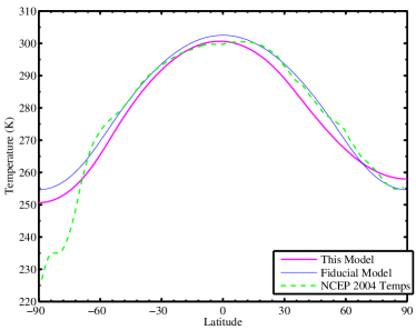
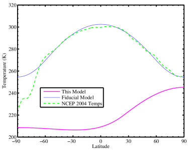
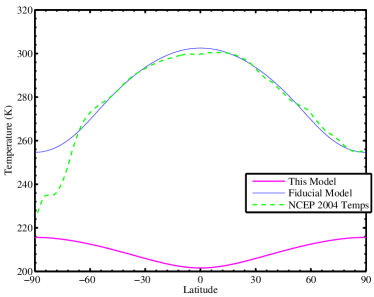
In SMS08, we verified that our “fiducial” model (70% ocean; cooling-albedo functions) at 1 AU predicts temperatures that match the Earth’s actual temperature distribution at all latitudes that are not significantly affected by Antarctica (i.e., north of S or so). This indicates that the model accounts for the overall (annual) planetary energy balance reasonably well. Another obvious test is whether the model correctly predicts the monthly energy fluxes that together go into the overall balance. Because our current investigation tests the influence of obliquity on climate, and obliquity is the primary driver of the Earth’s seasons, verifying the seasonal predictions of our model, given Earth-like conditions, is particularly relevant.
The diffusion equation model is a statement of conservation of energy. By definition, after vertical integration for a thin atmosphere with dominant surface processes,
| (3) |
where is the energy surface density (internal energy per unit surface area on the globe). The diffusion equation, therefore, says that the rate of change of internal energy at a given point equals the sources of energy (insolation), minus the sinks (infrared radiation), minus whatever energy flows away from the point under consideration.
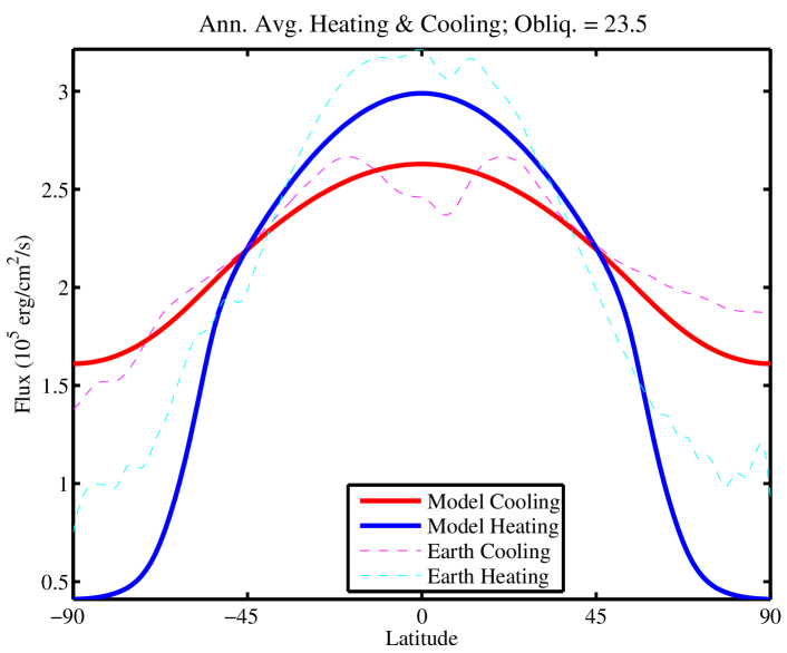
Figure 1 presents a comparison between the annually averaged fluxes of incoming and outgoing radiative energy in the fiducial model with the corresponding fluxes on Earth, taken from NASA’s Earth Radiation Budget Experiment (ERBE) in the mid-1980s (Barkstrom et al., 1990).222The ERBE satellite measured short-wavelength, or incoming, flux as that from 0.2 m to 4.5 m. Long-wavelength, or outgoing, flux was defined as all other flux within the bolometric range of the instrument. While our model does not capture the full shape of the Earth’s cooling and heating functions – in particular, the annually averaged model heating function is a bit below the Earth’s at the poles – still, both cooling and heating fluxes are within 10% of the Earth’s over most of the planet’s surface.
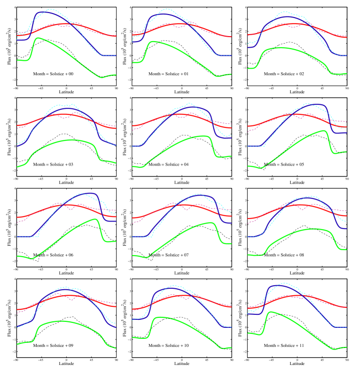
Figure 2 offers an even more compelling validation. In this figure, each of the 12 panels shows solar (i.e., heating), terrestrial (i.e., cooling), and net (solar minus terrestrial) radiative fluxes as functions of latitude, averaged over one month. Not only are our annually averaged cooling and heating functions in reasonable agreement with Earth’s, as per Figure 1, but furthermore the temporal variability of radiative fluxes in our model is similar to that of Earth.
For example, at the Northern winter solstice (upper left panel of Fig. 2), the model heating curve closely traces that of the Earth. It peaks at a somewhat more Southern latitude than the Earth’s does, but is within 10% of the Earth’s at all latitudes north of S. As the months advance, the concordance between the model heating curve and the Earth’s heating curve increases, until there is maximum agreement (within 10% at all atitudes) at the equinox (“Solstice+03”). Then, by the next solstice, the curves agree to within 10% at all latitudes South of roughly N. In a comparison of the cooling curves, the model shows even greater agreement with the data. In a majority of months, these two curves are within 10% of each other at all latitudes.
Interestingly, the month-by-month variations in model heating and model cooling lead to a net heating curve (heating minus cooling) that predicts some detailed features actually seen in the Earth’s net heating budget. Notice, for instance, the slight upward turn of the net heating curves of both the model and the Earth near the North Pole, at and around the Northern winter solstice. A similar feature is seen in both curves (though with slightly less impressive detailed agreement) near the South Pole, at and around the Southern winter solstice. These comparisons establish that our climate model exhibits reasonable regional and seasonal variability of not just temperature but also incoming and outgoing radiative energy fluxes.
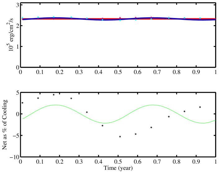
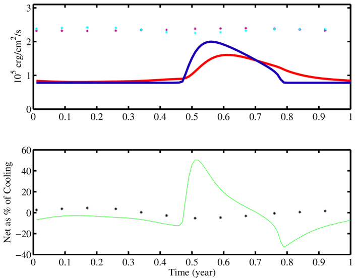
Another way to consider seasonal variations of heating and cooling fluxes is to look at the globe–average of each with respect to time. Figure 3 presents a comparison of these fluxes, for our fiducial model and the Earth itself. The bottom panel of this figure shows the net heating flux as a function of time of year, measured in fraction of a year from the Northern winter solstice. Earth’s net heating flux varies by about 5% with respect to the cooling flux, while our model’s varies somewhat less. The heating function for the Earth exceeds the cooling function during Northern winter for two main reasons:333Note that the cooling function, which traces surface temperatures, varies less through the seasonal cycle than the heating function. First, the nonzero eccentricity () of the Earth’s orbit places its perihelion – which occurs during Northern winter – approximately 3.4% closer to the Sun than its aphelion. This is responsible for of the annual annual variation in net heating flux. Our fiducial model, on the other hand, assumes zero eccentricity. Another contributing factor is that the Earth’s oceans on average absorb somewhat more insolation than the land, and the Southern hemisphere – which faces the Sun during Northern winter – has greater ocean coverage than the Northern hemisphere. To within , however, the Earth remains in global radiative balance throughout its seasonal cycle.
So far we have considered the radiative fluxes, but what about diffusive energy flux? We may combine equation (1) with equation (3) to produce:
| (4) |
where we have substituted for . Comparing equation (4) to a diffusion equation in spherical coordinates, and accounting for vertical integration, shows that is the rate of latitudinal energy transport per unit longitudinal length. The total rate of meridional diffusive heat transport (i.e. energy crossing a given latitude circle per unit time) therefore is
| (5) |
Figure 4 shows profiles of this diffusive heat transport rate in our fiducial model, at Earth-like obliquity and at extreme obliquity. In the Earth-like configuration, heat flows from the equator toward the poles. In the highly oblique configuration, however, heat flows in the other direction, from the poles to the equator (in an annually averaged sense). For comparison, Williams & Pollard (2003) present a full general circulation model (GCM) of an Earth-like planet at Earth-like and higher obliquity. Figure 2 of that paper shows the meridional heat flux within their models for obliquity and obliquity, and the results are strikingly similar to ours. At obliquity, our model’s diffusive flux is very close to that of the GCM. At high obliquity, the flux in our model remains within of that in the GCM (from visual inspection), at all latitudes. This reasonable concordance indicates that the treatment of heat transport within our model, despite being very simple, is still likely to remain useful as a representation of heat transport in less-Earth-like conditions. We emphasize that it is a nontrivial point that this entirely different regime of transport should remain well-captured by a diffusion approximation.
4 Study of Habitability
For model planets with obliquity on a circular orbit at 1 AU, both pairs of infrared cooling functions and albedo functions presented in Table LABEL:obl_tab:one are reasonably good matches for the Earth’s current climate, as measured by latitudinally averaged temperatures, with a somehwat better fit with . This gives us some confidence that these functions are useful guides as to how the climate might respond under different forcing conditions. In this investigation, we consider how variations in intrinsic planetary characteristics combine with the changes in insolation and year-length at various orbital radii to map the zone of regionally habitable climates on planets with various obliquities.
We follow SMS08 in saying that, at a given time, a part of a planet is habitable if its surface temperature is between 273 K and 373 K, corresponding to the freezing and boiling points of pure water at 1 Atm pressure. This criterion may be criticized for several reasons discussed in SMS08 and references therein, but it provides a reasonable starting point for making numerical investigations. We will frequently quantify habitability of pseudo-Earths with the temporal habitability fraction, , where is orbital semimajor axis, is latitude, and is the fraction of the year that the point in parameter space specified by spends in the habitable temperature range (see SMS08 for details).
4.1 Efficiency of Heat Transport
Terrestrial planets with different rotation rates will redistribute heat from the substellar point (or, in a 1D model, the substellar latitude) with different efficiencies. According to the idealized scaling described above, wherein the effective diffusion coefficient varies with the inverse square of the planetary rotation rate, slower spinning planets will redistribute heat more efficiently, while faster spinning planets will do so less efficiently. But from where, and to where, is heat redistributed? How does this depend on obliquity and rotation rate? And what influence does this have on climatic habitability?
4.1.1 Direction of Heat Flow
For an Earth-like obliquity, the substellar latitude does not vary very much over the course of the year: the tropics are fairly close to the equator (the tropical region is less than one third of the Earth’s surface area). As a result, it is a reasonable approximation that heat is always being transported from the equator to the poles (but see Fig. 2 for details). In contrast, on a planet with significantly larger obliquity, the direction of heat flow changes over the course of the annual cycle. At the equinoxes, the equator is the most strongly insolated part of the planet (regardless of obliquity), and so heat builds up at the equator, to be partially redistributed by atmospheric motions. But on a highly oblique planet, polar summers are extremely intense, as measured by diurnally averaged insolation. As a result, heat builds up at the poles during their corresponding summers, and the flow of heat reverses direction.
Figure 5 demonstrates the effect of such strong polar summers on the global radiation budget of a model planet, by comparison to Figure 1 in which the annually averaged cooling and heating are shown for an Earth-like, obliquity model. As expected for the Earth-like model, over the annual cycle, the equator receives significantly more solar radiation than do the poles, and accordingly the annually averaged heating exceeds the cooling at the equator. This indicates that atmospheric motions transport heat poleward from the equator on average. In Figure 5, on the other hand, we present the analogous functions in the case of high and extreme obliquity models. The left panel shows the heating and cooling functions for a model at obliquity; the right panel shows the same functions for a model at obliquity. Planetary scientists have long recognized that in highly oblique models such as these, the polar summers are so intense that, averaged over the year, the most strongly insolated parts of the planet are the North and South Poles! (See, e.g., ward1974.) In an annually averaged sense, then, heat flows from the poles to the equator, although clearly the direction of flow changes with the seasons, as described above. The import of these plots is that our notion that the poles are the coldest planetary regions might have to be revised in the case of highly oblique worlds. The resulting regime of atmospheric transport, which is only parameterized with our diffusive treatment, may also be expected to differ substantially from that on Earth (e.g., in terms of equatorial Hadley cells).
Figure 6 shows in greater detail the extreme way in which insolation can vary over the annual cycle in a highly oblique model. In this model, the obliquity of an otherwise Earth-like planet (– functions, with 70% ocean uniformly distributed) is set to 90. Notice that the cooling remains much more steady than the heating in this model. This is because of the high effective heat capacity of the atmosphere above ocean. In models with less ocean coverage, or oceans that are nonuniformly distributed, the cooling too can vary dramatically over the annual cycle.444It is also worth noting that at the outer reaches of a star’s habitable zone (e.g., Kasting et al., 1993), the annual cycle might be long enough relative to the thermal timescale ( a decade) of the ocean-atmosphere mixed layer that it could undergo relatively large swings in temperature within a single annum. Because the heating varies so intensely while the cooling varies less, their difference – the net heating curve – also exhibits large variations within the annual cycle. At each solstice, the pole facing the star receives far more net radiant flux than both the opposite pole and the planetary mean. At the equinoxes, something perhaps more surprising happens: the net radiant flux is negative over much of the model planet’s surface, and only barely positive near the equator. Overall, the planet heats strongly at the poles during solstices (while cooling elsewhere) and either cools or remains essentially thermally neutral everywhere during equinoxes.
4.1.2 Implications for Habitability
As SMS08 demonstrates, model planets with efficient heat transport (slowly spinning planets) are more latitudinally isothermal than models with Earth-like rotation, which themselves exhibit less latitudinal variation of temperature than those with inefficient heat transport (fast spinning planets). As a result, models corresponding to worlds that are spinning slowly relative to the Earth (but still fast enough that a 1-D climate model has some use) tend to be either entirely habitable or entirely non-habitable at any given time. In contrast, Earth-like and faster spinning model planets may be only partially habitable at a particular time. They may, for instance, be frozen at the poles and temperate at the equator, or vice versa in the case of a highly oblique world.
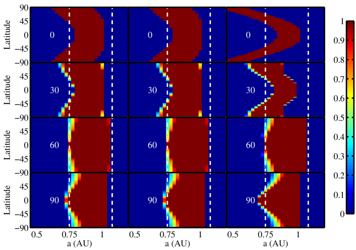
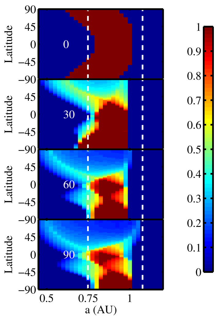
Figure 7 demonstrates the complicated interplay that can go on between obliquity and efficiency of heat transport, in determining a planet’s habitability. This figure shows the temporal habitability fraction, as a function of orbital semimajor axis and latitude, for each of 12 different combinations of obliquity (, , , ) and latitudinal heat diffusion coefficient (, , and , corresponding respectively to 72-hour, 24-hour, 8-hour rotations). The top panel shows these plots for the () cooling–albedo pair, and the bottom panel depicts the () pair (see Table LABEL:obl_tab:one for details). In both panels, the left column of plots represents efficient latitudinal heat transport; the middle column represents Earth-like transport; and the right column represents inefficient transport. Each of the 24 plots in this figure shows the results of model runs for planets located from AU to 1.25 AU in increments of AU. The color scale indicates the fraction of the year that the latitude at that point spends in the habitable temperature range (273 K - 373 K) on a model planet at the specified orbital semimajor axis. In each plot, the white vertical dashed lines indicate the radiative equilibrium habitable zone, calculated (as discussed in SMS08) from a 0-dimensional model with annually averaged, globally averaged insolation and cooling.
There are a number of interesting features in Figure 7. The most obvious one is that, as expected, at every obliquity, less efficient transport results in more strongly latitudinally differentiated temporal habitability. In addition, at each transport-efficiency value, the sign shape of the seasonally habitable ribbon at low obliquity reverses to a sign shape at high obliquity. In other words, at low obliquity, the relatively cold poles are habitable closer to the star and the relatively warm equator is habitable farther from the star. At high obliquity, however, this reverses and the poles are relatively warm, while the equator is comparatively colder.
Furthermore, in both panels, the contours in most cells show a very abrupt outer boundary to the seasonally habitable zone. This is because, as discussed in SMS08, the ice-albedo feedback renders these models quite sensitive to changes in forcing. Small reductions in insolation can be amplified, because the ice-coverage increases, which increases the global albedo and leads to further reduction in insolation. This feedback mechanism renders the model climates susceptible to a global snowball transition, from which they cannot recover within our model framework. 555Additional feedback mechanisms that are not incorporated in our model exist on a real planet and might help it to recover from a snowball state. For discussions of how the Earth might have recovered from one or more snowball episodes, see, for example, caldeira+kasting1992, Hoffman & Schrag (2002), and pierrehumbert2004. The main exceptions to this trend are the low obliquity, fast-spinning models, in the upper right corners of both panels, although even these models drop to 0% habitability at orbital radii that are small relative to the outer boundary of the habitable zone set by global radiative equilibrium (indicated by the white dashed lines). Interestingly, the fairly small difference in cooling–albedo functions from () to () is sufficient to allow the cell in the lower right corner of the bottom panel – extreme obliquity, inefficient transport – to avoid transitioning globally to a snowball state. In that model, the intense summer insolation at the poles, combined with the relative thermal isolation of different latitudes, allows the poles to heat up above the freezing point of water during their summers, even at orbital distances where other models would be entirely frozen. In sum, susceptibility to snowball transitions depends on details of parameterizations in our energy balance model, as has been noted before for Earth climate studies (e.g., North et al., 1981).
4.2 Land/Ocean Distribution
As described in SMS08, the large covering fraction of oceans on the Earth (roughly 70%) stabilizes our climate over an annual cycle, by virtue of the large effective heat capacity of atmosphere over ocean. Over land, the thermal relaxation timescale is several months, while for the ( m deep) mixed layer over the ocean, the thermal relaxation timescale is more than a decade. As a result, in a 1D model (such as ours) that does not resolve continents in longitude, any latitude band with significant ocean fraction will have strongly suppressed annual temperature variations relative to a latitude band with low ocean fraction. Because we do not know of any way to determine a priori the distribution of continents and oceans on an extrasolar planet, it is important to consider the influence on climatic habitability of other possible land/ocean distributions.
4.2.1 Nonuniform Ocean Coverage
We consider model planets with distributions of land and ocean that are not uniform across different latitudes: one with 30% land coverage, with a land-mass centered on the North Pole (extending down to North latitude), and the other (discussed in § 4.2.2) with 90% land, again centered on the North Pole.666Equivalently, this model can be conceived as having an ocean centered at the South Pole. Because of the relatively low thermal inertia of atmosphere over land, parts of a model planet that are dominated by land can freeze or boil during the course of the year and still return to temperate conditions at other times. In fact, at some orbital distances, and at high obliquity, the polar regions of some models freeze and boil within an annual cycle.
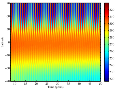
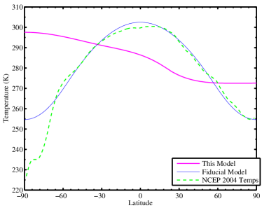
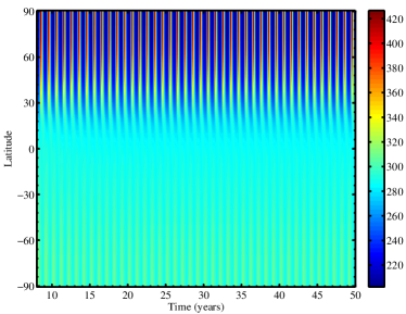
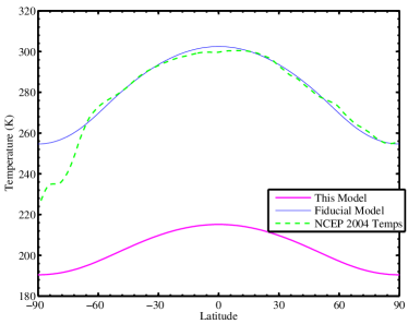
Figure 8 displays the tremendous swings of temperature that can occur over latitude bands that lack ocean, and also indicates that annually averaged calculations can miss a lot of information about instantaneous conditions on oblique planets. This figure contrasts the annually averaged temperature with the detailed temperature evolution on a model planet with a North Polar continent that is 30% of the total surface area, at an orbital distance of 1 AU. This model uses () cooling–albedo functions and results are shown for obliquities , , and . At all three obliquities, the left column – the annually averaged temperature profile – provides an impoverished view of the actual climatic conditions. Looking at just the left panels: the obliquity model appears slightly asymmetrical in temperature distribution, with the continental North Pole 8 K warmer than the oceanic South Pole; the obliquity model appears cooler at the continental pole; and the obliquity model again appears warmer at the continental pole, but appears frozen over the whole globe. In truth, all three models reach significantly higher temperatures at the continental pole during its summer than at the other pole. At both and obliquity, North Pole summer temperatures exceed 410 K, as the Sun shines nearly straight down on the pole for months. We note that an important limitation of our models is apparent in this figure. Although we may not have much intuition for what the polar summers should be like on high obliquity planets, it is surprising to obtain summer polar continent temperatures in excess of 310 K in the obliquity model. Indeed, Antarctica – Earth’s continental pole – is significantly colder than the non-continental pole, and for the most part neither pole ever reaches temperatures above freezing. Accounting for Antarctica in our model framework would be non-trivial, as it may require initial conditions differing from uniformly ice-free and/or improved treatments of ice-related surface processes.
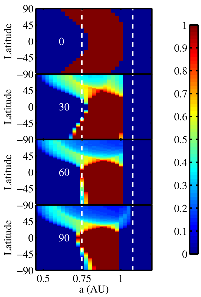
Figure 9 presents plots of the temporal habitability fraction for the same model planet as above, at obliquities , , , . Figure 8 illustrated how the presence of land at the North Pole causes tremendous swings in temperature there; Fig. 9 confirms that, for nonzero obliquity, this is indeed the case throughout the orbital extent of the habitable zone. These large seasonal variations lead to exotic shapes in plots of temporal habitability. Compared with uniformly ocean-dominated worlds, much more of the parameter space is partially habitable at each obliquity (except ), neither 0% nor 100% of the year, but somewhere in between.
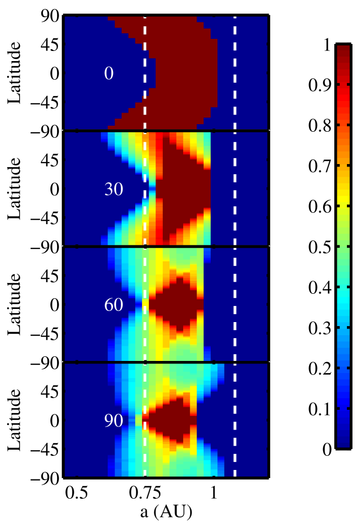
4.2.2 Desert Worlds
We now consider two model planets with just 10% ocean fraction. We examine the cases of a uniformly distributed ocean (10% in every latitude band) and an ocean localized at the South Pole (extending northward to South latitude). Figure 10 presents the temporal habitability for the uniform desert world, while Figure 11 presents the analogous plot for the desert world with a South Polar ocean. As before, some regions of these model planets swing from freezing to boiling temperatures over the course of the year. This is responsible for the butterfly shape of the temporal habitability plots in the and obliquity cases shown in Fig. 10: at , the poles are habitable for a smaller fraction of the year than more equatorial regions at that orbital distance, or than the poles for closer and more distant orbits. The pattern of habitability in Fig. 11, on the other hand, shows how strongly assymmetric the climate can be on a desert world with a polar ocean.
These models, and those presented in § 4.2.1, suggest that at extreme obliquity the inner edge of the zone of regionally and seasonally habitable climates can be extended dramatically inward, while the outer boundary can only be extended mildly outward. Several important caveats should accompany this observation, however. Assuming an infrared cooling function that is constant with orbital radius probably leads to a flawed treatment at both the high and low insolation limits of these models. At the inner edge of the habitable zone, large increases in atmospheric water content can cause a reduction in the cooling efficiency, leading to a runaway greenhouse effect. An eventual catastrophic water loss can result in a Venus-like outcome, as described by Kasting et al. (1993) and references therein (although this type of outcome might be mitigated by reduced heating from increased cloud-albedo, as mentioned in SMS08). At the outer edge, on long timescales, a reduced efficiency of the carbonate-silicate weathering cycle is likely to lead to a significant increase in the partial pressure of atmospheric CO2 (Kasting et al., 1993), which could extend the habitable zone from , as in our models, to or beyond in some cases. We discuss in greater detail the issue of varying atmospheric CO2 content with orbital distance in § 4.3.
Notwithstanding these various complications, for plausible cooling functions, the low thermal inertia of atmosphere over land might lead to severe polar climates on highly oblique planets. What are we to make of partial “habitability” by our criterion in the case of a region of a planet that actually boils and freezes every year? There are some microbes on Earth that can reproduce at freezing temperatures, and others that can reproduce at boiling temperatures (see SMS08 and references therein), although none of which we are aware that can do both. If part of a planet regularly swings through these wild extremes of climate, is it appropriate to call it habitable? More relevant from the perspective of formulating a testable scientific hypothesis, could such a planet support enough life to produce sufficient levels of biosignatures that its life could be detected from Earth? This is an open question, but it is worthwhile to keep in mind that microbes on Earth appear to be as hardy as they need to be: nearly everywhere that biologists have searched, they have found some microbes thriving. A perhaps equally significant result from the perspective of habitability is that the reduced thermal inertia of these models appears to render them somewhat less susceptible to global snowball events, especially at high obliquities (e.g., compare Figs. 9-11 with the middle column of Fig. 7).
4.3 Modeling the Far Reaches of the Habitable Zone
Walker et al. (1981) propose that a planet’s temperature is regulated on long timescales by a feedback mechanism involving weathering of silicate rocks through carbonic acid from CO2 disolved in water. They argue that since the rate of weathering (and hence of removal of CO2 from the atmosphere) increases with temperature, this process is an important negative feedback on climate that acts to keep temperatures near the freezing point of water (see the recent study by zeebe+caldeira2008 confirming the operation of this cycle). Kasting et al. (1993) point out that this negative feedback can significantly offset the extreme sensitivity of climate to changes in orbital distance away from 1 AU seen in models such as those of Hart (1979) and the models presented in SMS08 and thus far in this paper. These models are sensitive because they contain a significant positive feedback of the Earth-climate – the ice-albedo feedback whereby at lower temperatures the absorbed insolation is dramatically reduced because of the high albedo of ice. However, these models also ignore the long-term, negative (counterbalancing) feedback of the carbonate-silicate weathering cycle (Kasting et al., 1993).
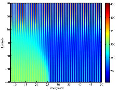
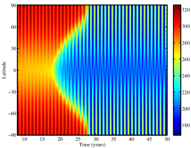
In order to probe the combined influence on climate of rotation rate and obliquity in the context of the expected CO2-rich atmosphere that a pseudo Earth would have at 1.4 AU, we switch to the infrared cooling function used by WK97 ( in Table LABEL:obl_tab:one), with CO2 partial pressure (CO2) set to 1 bar and 2 bars. For simplicity, we maintain the same albedo function as before and adopt the same linear dependence of the latitudinal heat diffusion coefficient with total atmospheric pressure as WK97 (). We find that at both 1- and 2-bar levels of CO2, model planets maintain globally temperate conditions at all obliquities for both and – corresponding to slow and Earth-like rotation. Interestingly, however, at reduced transport efficiency, corresponding to fast planetary rotation, we find that these CO2-rich models are susceptible to global glaciation events.
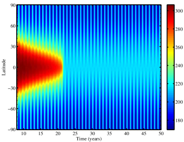
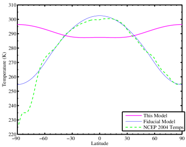
Figure 12 shows the global average temperature and the climate evolution for fast-spinning model planets at 1.4 AU with 1 bar atmospheric CO2, () cooling-albedo functions and a latitudinal heat diffusion coefficient scaled up with total pressure but reduced by a factor 9 to account for rapid rotation. At obliquity, the cold temperatures at the poles drag the model into a snowball state, while at obliquity, it is the cold equator that drags the model planet to the same fate. At obliquity, however, no part of the planet receives consistently low enough insolation to trigger global glaciation. The snowball effect seen in the and obliquity models might be particularly dramatic because of the possibility of partial atmospheric collapse, on a much shorter timescale than volcanism can replenish CO2. At 1 bar, the freezing point of CO2 is . Both the and obliquity models reach temperatures below this threshold over large enough regions of their surfaces777The very large seasonal variations of temperature on these snowball planets result from the moderate heat capacity of the atmosphere over ice (see, e.g., SMS08; WK97). that significant amounts of the atmospheric CO2 might condense out as dry ice, thereby reducing the atmospheric greenhouse effect. The risk of atmospheric collapse would be somewhat lessened by the release of latent heat from CO2 condensation, which would tend to prevent too much CO2 from freezing out during any winter. Partial collapse, on the other hand, would reduce surface pressure and thus the efficiency of atmospheric heat transport. Realistically treating these possibilities is beyond the scope of the present paper as it would require incorporating a latent heat term in the energy balance equation and accounting for the surface CO2 mass budget, as Nakamura & Tajika (2002) do in their Mars EBM.
While model runs with 2 bars of CO2 (not shown) indicate that a pseudo-Earth with such a massive atmosphere at 1.4 AU would be unlikely to suffer glaciation or partial atmospheric collapse at any obliquity, it is worth noting that on a planet with a rate of volcanic greenhouse gas output not much higher than on Earth, it may be difficult to build up a thick CO2 atmosphere (e.g., 2 bars) under conditions such that CO2 condenses out at lower pressure (like in our model with 1 bar of CO2). In situations in which atmospheric CO2 concentrations can change appreciably on a yearly timescale, our model is not self-consistent. Further analysis is therefore needed to determine the full extent and consequences of such atmospheric condensation events. Clearly, these various issues are important subjects for future studies since they indicate that snowball transitions could in principle limit the habitability of some terrestrial planets by interfering with the negative feedback of their carbonate-silicate weathering cycles.
4.4 Validity of Global Radiative Balance
Calculations of habitable zones have often assumed global radiative balance conditions. Although these calculations by definition cannot account for the regional character of habitability, one might hope that they still provide a decent proxy for the global average conditions. Indeed, as seen in Fig. 3, the Earth itself is within of radiative equilibrium throughout the year. Accordingly, global radiative balance models have provided a very useful starting point for considerations of how the habitability of an Earth-like planet depends on its orbital radius.
Figure 13 presents globally averaged cooling, heating, and net radiative fluxes in a model with a North Polar continent that covers 30% of the planet’s surface, with obliquity. In contrast to the Earth, which remains within of global radiative balance, this model planet can be nearly 60% out of global radiative balance. While it has been recognized that planets on highly eccentric orbits experience forcings that are significantly different from annually and globally averaged conditions, the results in Fig. 13 illustrate how, even on circular orbits, planets can experience conditions that are far from radiative equilibrium. This further underscores the importance of regional, time-dependent climate models for addressing the habitability of extrasolar terrestrial planets.
5 Conclusions
We have presented a series of energy balance models to address the variety of climatic conditions that might exist on oblique terrestrial planets with circular orbits. We considered dynamic climate forcings and responses determined by several planetary attributes a priori unknown for extrasolar planets, including obliquity, rotation rate, distribution of land/ocean coverage, and the detailed nature of the radiative cooling and heating functions. We find that planets with small ocean fractions or polar continents can experience very severe seasonal climatic variations, but that these planets also might maintain seasonally and regionally habitable conditions over a larger range of orbital radii than more Earth-like planets. Climates on high obliquity planets with nonuniform distributions of land and ocean can be far from global radiative balance, as compared to the Earth. Our results provide indications that the modeled climates are somewhat less prone to dynamical snowball transitions at high obliquity. Fast rotating Earth-like planets may fall victim to global glaciation events at closer orbital radii than slower rotating planets. This is also the case for planets with massive CO2 atmospheres, which are expected to be found in the outer orbital range of habitable zones. Snowball transitions could be particularly significant for such planets since partial collapse of their CO2-rich atmospheres may occur and possibly interfere with the thermostatic effect of their carbonate-silicate weathering cycle, thus affecting their long-term habitability.
Acknowledgments
We acknowledge helpful conversations with James Cho, Michael Allison, Anthony Del Genio, and Scott Gaudi. We thank Diana Spiegel for help with ERBE data. We acknowledge many useful comments by an anonymous referee. CS acknowledges the funding support of the Columbia Astrobiology Center through Columbia University’s Initiatives in Science and Engineering, and a NASA Astrobiology: Exobiology and Evolutionary Biology; and Planetary Protection Research grant, # NNG05GO79G.
| Model | IR Cooling Function | Albedo Function |
|---|---|---|
| 2aa Model with –dependent optical thickness: . | ||
| 3bb Linearized model: , . | ||
| 4cc WK97 cooling function (with albedo). The detailed functional form is presented in the appendix of WK97. |


References
- Baglin (2003) Baglin, A. 2003, Advances in Space Research, 31, 345
- Barkstrom et al. (1990) Barkstrom, B. R., Harrison, E. F., & Lee, III, R. B. 1990, EOS Transactions, 71, 279
- Barnes et al. (2008) Barnes, R., Raymond, S. N., Jackson, B., & Greenberg, R. 2008, ArXiv e-prints, 807
- Basri et al. (2005) Basri, G., Borucki, W. J., & Koch, D. 2005, New Astronomy Review, 49, 478
- Beatty & Gaudi (2008) Beatty, T. G. & Gaudi, B. S. 2008, ArXiv e-prints, 804
- Beaulieu et al. (2006) Beaulieu, J.-P., Bennett, D. P., Fouqué, P., Williams, A., Dominik, M., Jorgensen, U. G., Kubas, D., Cassan, A., Coutures, C., Greenhill, J., Hill, K., Menzies, J., Sackett, P. D., Albrow, M., Brillant, S., Caldwell, J. A. R., Calitz, J. J., Cook, K. H., Corrales, E., Desort, M., Dieters, S., Dominis, D., Donatowicz, J., Hoffman, M., Kane, S., Marquette, J.-B., Martin, R., Meintjes, P., Pollard, K., Sahu, K., Vinter, C., Wambsganss, J., Woller, K., Horne, K., Steele, I., Bramich, D. M., Burgdorf, M., Snodgrass, C., Bode, M., Udalski, A., Szymański, M. K., Kubiak, M., Wiȩckowski, T., Pietrzyński, G., Soszyński, I., Szewczyk, O., Wyrzykowski, Ł., Paczyński, B., Abe, F., Bond, I. A., Britton, T. R., Gilmore, A. C., Hearnshaw, J. B., Itow, Y., Kamiya, K., Kilmartin, P. M., Korpela, A. V., Masuda, K., Matsubara, Y., Motomura, M., Muraki, Y., Nakamura, S., Okada, C., Ohnishi, K., Rattenbury, N. J., Sako, T., Sato, S., Sasaki, M., Sekiguchi, T., Sullivan, D. J., Tristram, P. J., Yock, P. C. M., & Yoshioka, T. 2006, Nature, 439, 437
- Bennett et al. (2008) Bennett, D. P., Bond, I. A., Udalski, A., Sumi, T., Abe, F., Fukui, A., Furusawa, K., Hearnshaw, J. B., Holderness, S., Itow, Y., Kamiya, K., Korpela, A. V., Kilmartin, P. M., Lin, W., Ling, C. H., Masuda, K., Matsubara, Y., Miyake, N., Muraki, Y., Nagaya, M., Okumura, T., Ohnishi, K., Perrott, Y. C., Rattenbury, N. J., Sako, T., Saito, T., Sato, S., Skuljan, L., Sullivan, D. J., Sweatman, W. L., Tristram, P. J., Yock, P. C. M., Kubiak, M., Szymanski, M. K., Pietrzynski, G., Soszynski, I., Szewczyk, O., Wyrzykowski, L., Ulaczyk, K., Batista, V., Beaulieu, J. P., Brillant, S., Cassan, A., Fouque, P., Kervella, P., Kubas, D., & Marquette, J. B. 2008, ArXiv e-prints, 806
- Borucki et al. (2003) Borucki, W. J., Koch, D., Basri, G., Brown, T., Caldwell, D., Devore, E., Dunham, E., Gautier, T., Geary, J., Gilliland, R., Gould, A., Howell, S., & Jenkins, J. 2003, in ESA Special Publication, Vol. 539, Earths: DARWIN/TPF and the Search for Extrasolar Terrestrial Planets, ed. M. Fridlund, T. Henning, & H. Lacoste, 69–81
- Borucki et al. (2007) Borucki, W. J., Koch, D. G., Lissauer, J., Basri, G., Brown, T., Caldwell, D. A., Jenkins, J. M., Caldwell, J. J., Christensen-Dalsgaard, J., Cochran, W. D., Dunham, E. W., Gautier, T. N., Geary, J. C., Latham, D., Sasselov, D., Gilliland, R. L., Howell, S., Monet, D. G., & Batalha, N. 2007, in Astronomical Society of the Pacific Conference Series, Vol. 366, Transiting Extrapolar Planets Workshop, ed. C. Afonso, D. Weldrake, & T. Henning, 309–+
- Chandler & Sohl (2000) Chandler, M. A. & Sohl, L. E. 2000, J. Geophys. Res., 105, 20737
- del Genio & Zhou (1996) del Genio, A. D. & Zhou, W. 1996, Icarus, 120, 332
- del Genio et al. (1993) del Genio, A. D., Zhou, W., & Eichler, T. P. 1993, Icarus, 101, 1
- Dole (1964) Dole, S. H. 1964, Habitable planets for man (New York, Blaisdell Pub. Co. [1964] [1st ed.].)
- Hart (1979) Hart, M. H. 1979, Icarus, 37, 351
- Hoffman & Schrag (2002) Hoffman, P. F. & Schrag, D. P. 2002, Terra Nova, 114, 129
- Hunt (1982) Hunt, B. G. 1982, J. Meteor. Soc. Japan, 60, 309
- Jenkins (2000) Jenkins, G. S. 2000, J. Geophys. Res., 105, 7357
- Jenkins (2001) —. 2001, J. Geophys. Res., 106, 32903
- Jenkins (2003) —. 2003, Journal of Geophysical Research (Atmospheres), 108, 4118
- Kalnay et al. (1996) Kalnay, E., Kanamitsu, M., Kistler, R., Collins, W., Deaven, D., Gandin, L., Iredell, M., Saha, S., White, G., Woollen, J., Zhu, Y., Chelliah, M., Ebisuzaki, W., Higgins, W., Janowiak, J., Mo, K. C., Ropelewski, C., Wang, J., Leetmaa, A., Reynolds, R., Jenne, R., & Joselph, D. 1996, Bull. Amer. Meteor. Soc., 77, 437
- Kasting & Catling (2003) Kasting, J. F. & Catling, D. 2003, ARA&A, 41, 429
- Kasting et al. (1993) Kasting, J. F., Whitmire, D. P., & Reynolds, R. T. 1993, Icarus, 101, 108
- Kistler et al. (1999) Kistler, R., Kalnay, E., Collins, W., Saha, S., White, G., Woollen, J., Chelliah, M., Ebisuzaki, W., Kanamitsu, M., Kousky, V., van del Dool, H., Jenne, R., & Fiorino, M. 1999, Bull. Amer. Meteor. Soc., 82, 247
- Laskar et al. (1993) Laskar, J., Joutel, F., & Robutel, P. 1993, Nature, 361, 615
- Laskar & Robutel (1993) Laskar, J. & Robutel, P. 1993, Nature, 361, 608
- Leger & Herbst (2007) Leger, A. & Herbst, T. 2007, ArXiv e-prints 0707.3385
- Mayor et al. (2008) Mayor, M., Udry, S., Lovis, C., Pepe, F., Queloz, D., Benz, W., Bertaux, J. ., Bouchy, F., Mordasini, C., & Segransan, D. 2008, ArXiv e-prints, 806
- Nakamura & Tajika (2002) Nakamura, T. & Tajika, E. 2002, Journal of Geophysical Research (Planets), 107, 5094
- Nakamura & Tajika (2003) —. 2003, Geophys. Res. Lett., 30, 18
- Neron de Surgy & Laskar (1997) Neron de Surgy, O. & Laskar, J. 1997, A&A, 318, 975
- North et al. (1981) North, G. R., Cahalan, R. F., & Coakley, Jr., J. A. 1981, Reviews of Geophysics and Space Physics, 19, 91
- North & Coakley (1979) North, G. R. & Coakley, J. A. 1979, in Evolution of Planetary Atmospheres and Climatology of the Earth, 249–+
- Oglesby & Ogg (1998) Oglesby, R. J. & Ogg, J. G. 1998, Paleoclimates, 2, 293
- Pierrehumbert (2005) Pierrehumbert, R. T. 2005, Journal of Geophysical Research (Atmospheres), 110, 1111
- Selsis et al. (2007) Selsis, F., Kasting, J. F., Levrard, B., Paillet, J., Ribas, I., & Delfosse, X. 2007, A&A, 476, 1373
- Shu (1982) Shu, F. H. 1982, The physical universe. an introduction to astronomy (A Series of Books in Astronomy, Mill Valley, CA: University Science Books, 1982)
- Spiegel et al. (2008) Spiegel, D. S., Menou, K., & Scharf, C. A. 2008, ApJ, 681, 1609
- Udry et al. (2007) Udry, S., Bonfils, X., Delfosse, X., Forveille, T., Mayor, M., Perrier, C., Bouchy, F., Lovis, C., Pepe, F., Queloz, D., & Bertaux, J.-L. 2007, A&A, 469, L43
- von Bloh et al. (2008) von Bloh, W., Bounama, C., Cuntz, M., & Franck, S. 2008, in IAU Symposium, Vol. 249, IAU Symposium, 503–506
- Walker et al. (1981) Walker, J. C. G., Hays, P. B., & Kasting, J. F. 1981, J. Geophys. Res., 86, 9776
- Williams & Kasting (1997) Williams, D. M. & Kasting, J. F. 1997, Icarus, 129, 254
- Williams et al. (1996) Williams, D. M., Kasting, J. F., & Caldeira, K. 1996, in Circumstellar Habitable Zones, ed. L. R. Doyle, 43–+
- Williams & Pollard (2003) Williams, D. M. & Pollard, D. 2003, International Journal of Astrobiology, 2, 1
- Williams (1988a) Williams, G. P. 1988a, Climate Dynam., 2, 205
- Williams (1988b) —. 1988b, Climate Dynam., 3, 45