Linear Coloring and Linear Graphs 

Department of Computer Science, University of Ioannina

P.O.Box 1186, GR-45110  Ioannina, Greece

{kioannid, stavros}@cs.uoi.gr

Abstract:  Motivated by the definition of linear coloring on simplicial complexes, recently introduced in the context of algebraic topology [10], and the framework through which it was studied, we introduce the linear coloring on graphs. We provide an upper bound for the chromatic number $\chi(G)$, for any graph $G$, and show that $G$ can be linearly colored in polynomial time by proposing a simple linear coloring algorithm. Based on these results, we define a new class of perfect graphs, which we call co-linear graphs, and study their complement graphs, namely linear graphs. The linear coloring of a graph $G$ is a vertex coloring such that two vertices can be assigned the same color, if their corresponding clique sets are associated by the set inclusion relation (a clique set of a vertex $u$ is the set of all maximal cliques containing $u$); the linear chromatic number $\mathcal{\lambda}(G)$ of $G$ is the least integer $k$ for which $G$ admits a linear coloring with $k$ colors. We show that linear graphs are those graphs $G$ for which the linear chromatic number achieves its theoretical lower bound in every induced subgraph of $G$. We prove inclusion relations between these two classes of graphs and other subclasses of chordal and co-chordal graphs, and also study the structure of the forbidden induced subgraphs of the class of linear graphs.

Keywords:  Linear coloring, chromatic number, linear graphs, co-linear graphs, chordal graphs, co-chordal graphs, strongly chordal graphs, algorithms, complexity.

1 Introduction

Framework-Motivation. A linear coloring of a graph $G$ is a coloring of its vertices such that if two vertices are assigned the same color, then their corresponding clique sets are associated by the set inclusion relation; a clique set of a vertex $u$ is the set of all maximal cliques in $G$ containing $u$. The linear chromatic number $\mathcal{\lambda}(G)$ of $G$ is the least integer $k$ for which $G$ admits a linear coloring with $k$ colors.

Motivated by the definition of linear coloring on simplicial complexes associated to graphs, first introduced by Civan and Yalçin [10] in the context of algebraic topology, we define the linear coloring on graphs. The idea for translating their definition in graph theoretic terms came from studying linear colorings on simplicial complexes which can be represented by a graph. In particular, we studied the linear coloring on the independence complex $\mathcal{I}(G)$ of a graph $G$, which can always be represented by a graph and, more specifically, is identical to the complement graph ${\overline{G\mkern 3.0mu}\mkern-3.0mu}{}$ of $G$ in graph theoretic terms; indeed, the facets of $\mathcal{I}(G)$ are exactly the maximal cliques of ${\overline{G\mkern 3.0mu}\mkern-3.0mu}{}$. However, the two definitions cannot always be considered as identical since not in all cases a simplicial complex can be represented by a graph; such an example is the neighborhood complex $\mathcal{N}(G)$ of a graph $G$. Recently, Civan and Yalçin [10] studied the linear coloring of the neighborhood complex $\mathcal{N}(G)$ of a graph $G$ and proved that, for any graph $G$, the linear chromatic number of $\mathcal{N}(G)$ gives an upper bound for the chromatic number of the graph $G$. This approach lies in a general framework met in algebraic topology.

In the context of algebraic topology, one can find much work done on providing boundaries for the chromatic number of an arbitrary graph $G$, by examining the topology of the graph through different simplicial complexes associated to the graph. This domain was motivated by Kneser’s conjecture, which was posed in 1955, claiming that “if we split the $n$-subsets of a $(2n+k)$-element set into $k+1$ classes, one of the classes will contain two disjoint $n$-subsets” [17]. Kneser’s conjecture was first proved by Lovász in 1978, with a proof based on graph theory, by rephrasing the conjecture into “the chromatic number of Kneser’s graph $KG_{n,k}$ is $k+2$” [18]. Many more topological and combinatorial proofs followed the interest of which extends beyond the original conjecture [22]. Although Kneser’s conjecture is concerned with the chromatic numbers of certain graphs (Kneser graphs), the proof methods that are known provide lower bounds for the chromatic number of any graph [19]. Thus, this initiated the application of topological tools in studying graph theory problems and more particularly in graph coloring problems [11].

The interest to provide boundaries for the chromatic number $\chi(G)$ of an arbitrary graph $G$ through the study of different simplicial complexes associated to $G$, which is found in algebraic topology bibliography, drove the motivation for defining the linear coloring on the graph $G$ and studying the relation between the chromatic number $\chi(G)$ and the linear chromatic number $\lambda({\overline{G\mkern 3.0mu}\mkern-3.0mu}{})$. We show that for any graph $G$, $\lambda({\overline{G\mkern 3.0mu}\mkern-3.0mu}{})$ is an upper bound for $\chi(G)$. The interest of this result lies on the fact that we present a linear coloring algorithm that can be applied to any graph $G$ and provides an upper bound $\lambda({\overline{G\mkern 3.0mu}\mkern-3.0mu}{})$ for the chromatic number of the graph $G$, i.e. $\chi(G)\leq\lambda({\overline{G\mkern 3.0mu}\mkern-3.0mu}{})$; in particular, it provides a proper vertex coloring of $G$ using $\lambda({\overline{G\mkern 3.0mu}\mkern-3.0mu}{})$ colors. Additionally, recall that a known lower bound for the chromatic number of any graph $G$ is the clique number $\omega(G)$ of $G$, i.e. $\chi(G)\geq\omega(G)$. Motivated by the definition of perfect graphs, for which $\chi(G_{A})=\omega(G_{A})$ holds $\forall A\subseteq V(G)$, it was interesting to study those graphs for which the equality $\chi(G)=\lambda({\overline{G\mkern 3.0mu}\mkern-3.0mu}{})$ holds, and even more those graphs for which this equality holds for every induced subgraph. The outcome of this study was the definition of a new class of perfect graphs, namely co-linear graphs, and, furthermore, the study of the classes of co-linear graphs and of their complement class, namely linear graphs.

Our Results. In this paper, we first introduce the linear coloring of a graph $G$ and study the relation between the linear coloring of ${\overline{G\mkern 3.0mu}\mkern-3.0mu}{}$ and the proper vertex coloring of $G$. We prove that, for any graph $G$, a linear coloring of ${\overline{G\mkern 3.0mu}\mkern-3.0mu}{}$ is a proper vertex coloring of $G$ and, thus, $\lambda({\overline{G\mkern 3.0mu}\mkern-3.0mu}{})$ is an upper bound for $\chi(G)$, i.e. $\chi(G)\leq\lambda({\overline{G\mkern 3.0mu}\mkern-3.0mu}{})$. We present a linear coloring algorithm that can be applied to any graph $G$. Motivated by these results and the Perfect Graph Theorem [15], we study those graphs for which the equality $\chi(G)=\lambda({\overline{G\mkern 3.0mu}\mkern-3.0mu}{})$ holds for every induce subgraph and define a new class of perfect graphs, namely co-linear graphs; we also study their complement class, namely linear graphs. A graph $G$ is a co-linear graph if and only if its chromatic number $\mathcal{\chi}(G)$ equals to the linear chromatic number $\mathcal{\lambda}({\overline{G\mkern 3.0mu}\mkern-3.0mu}{})$ of its complement graph ${\overline{G\mkern 3.0mu}\mkern-3.0mu}{}$, and the equality holds for every induced subgraph of $G$, i.e. $\mathcal{\chi}(G_{A})=\mathcal{\lambda}({\overline{G\mkern 3.0mu}\mkern-3.0mu}{}_{A})$, $\forall A\subseteq V(G)$; a graph $G$ is a linear graph if it is the complement of a co-linear graph. We show that the class of co-linear graphs is a superclass of the class of threshold graphs, a subclass of the class of co-chordal graphs and is distinguished from the class of split graphs. Additionally, we give some structural and recognition properties for the classes of linear and co-linear graphs. We study the structure of the forbidden induced subgraphs of the class of linear graphs, and show that any $P_{6}$-free chordal graph, which is not a linear graph, properly contains a $k$-sun as an induced subgraph. Therefore, we infer that the subclass of chordal graphs, namely linear graphs, is a superclass of the class of $P_{6}$-free strongly chordal graphs.

Basic Definitions. Some basic graph theory definitions follow. We consider finite undirected and directed graphs with no loops or multiple edges. Let $G$ be such a graph; then, $V(G)$ and $E(G)$ denote the set of vertices and of edges of $G$, respectively. An edge is a pair of distinct vertices $x,y\in V(G)$, and is denoted by $xy$ if $G$ is an undirected graph and by $\overrightarrow{xy}$ if $G$ is a directed graph. For a set $A\subseteq V(G)$ of vertices of the graph $G$, the subgraph of $G$ induced by $A$ is denoted by $G_{A}$. Additionally, the cardinality of a set $A$ is denoted by $|A|$. For a given vertex ordering $(v_{1},v_{2},\ldots,v_{n})$ of a graph $G$, the subgraph of $G$ induced by the set of vertices $\{v_{i},v_{i+1},\ldots,v_{n}\}$ is denoted by $G_{i}$. The set $N(v)=\{u\in V(G):(u,v)\in E(G)\}$ is called the open neighborhood of the vertex $v\in V(G)$ in $G$, sometimes denoted by $N_{G}(v)$ for clarity reasons. The set $N[v]=N(v)\cup\{v\}$ is called the closed neighborhood of the vertex $v\in V(G)$ in $G$. In a graph $G$, the length of a path is the number of edges in the path. The distance $d(v,u)$ from vertex $v$ to vertex $u$ is the minimum length of a path from $v$ to $u$; $d(v,u)=\infty$ if there is no path from $v$ to $u$.

The greatest integer $r$ for which a graph $G$ contains an independent set of size $r$ is called the independence number or otherwise the stability number of $G$ and is denoted by $\mathcal{\alpha}(G)$. The cardinality of the vertex set of the maximum clique in $G$ is called the clique number of $G$ and is denoted by $\mathcal{\omega}(G)$. A proper vertex coloring of a graph $G$ is a coloring of its vertices such that no two adjacent vertices are assigned the same color. The chromatic number $\mathcal{\chi}(G)$ of $G$ is the least integer $k$ for which $G$ admits a proper vertex coloring with $k$ colors. For the numbers $\mathcal{\omega}(G)$ and $\mathcal{\chi}(G)$ of an arbitrary graph $G$ the inequality $\mathcal{\omega}(G)\leq\mathcal{\chi}(G)$ holds. In particularly, $G$ is a perfect graph if the equality $\mathcal{\omega}(G_{A})=\mathcal{\chi}(G_{A})$ holds $\forall A\subseteq V(G)$. For more details on basic definitions in graph theory refer to [6, 15].

Next, definitions of some graph classes mentioned throughout the paper follow. A graph is called a chordal graph if it does not contain an induced subgraph isomorphic to a chordless cycle of four or more vertices. A graph is called a co-chordal graph if it is the complement of a chordal graph [15]. A hole is a chordless cycle $C_{n}$ if $n\geq 5$; the complement of a hole is an antihole. A graph $G$ is a split graph if there is a partition of the vertex set $V(G)=K+I$, where $K$ induces a clique in $G$ and $I$ induces an independent set. Split graphs are characterized as $(2K_{2},C_{4},C_{5})$-free. Threshold graphs are defined as those graphs where stable subsets of their vertex sets can be distinguished by using a single linear inequality. Threshold graphs were introduced by Chvátal and Hammer [9] and characterized as $(2K_{2},P_{4},C_{4})$-free. Quasi-threshold graphs are characterized as the $(P_{4},C_{4})$-free graphs and are also known in the literature as trivially perfect graphs [15, 21]. A graph is strongly chordal if it admits a strong perfect elimination ordering. Strongly chordal graphs were introduced by Farber in [12] and are characterized completely as those chordal graphs which contain no $k$-sun as an induced subgraph. For more details on basic definitions in graph theory refer to [6, 15].

2 Linear Coloring on Graphs

In this section we define the linear coloring of a graph $G$, we prove some properties of the linear coloring of $G$, and present a simple algorithm for linear coloring that can be applied to any graph $G$. It is worth noting that similar properties of linear coloring of the neighborhood complex $\mathcal{N}(G)$ have been proved by Civan and Yalçin [10].

Definition 2.1. Let $G$ be a graph and let $v\in V(G)$. The clique set of a vertex $v$ is the set of all maximal cliques of $G$ containing $v$ and is denoted by $\mathcal{C}_{G}(v)$.

Definition 2.2. Let $G$ be a graph. A surjective map $\mathcal{\kappa}:V(G)\rightarrow[k]$ is called a $k$-linear coloring of $G$ if the collection $\{\mathcal{C}_{G}(v):\mathcal{\kappa}(v)=i\}$ is linearly ordered by inclusion for all $i\in[k]$, where $\mathcal{C}_{G}(v)$ is the clique set of $v$, or, equivalently, for two vertices $v,u\in V(G)$, if $\mathcal{\kappa}(v)=\mathcal{\kappa}(u)$ then either $\mathcal{C}_{G}(v)\subseteq\mathcal{C}_{G}(u)$ or $\mathcal{C}_{G}(v)\supseteq\mathcal{C}_{G}(u)$. The least integer $k$ for which $G$ is $k$-linear colorable is called the linear chromatic number of $G$ and is denoted by $\lambda(G)$.

2.1 Properties

Next, we study the linear coloring on graphs and its association to the proper vertex coloring. In particular, we show that for any graph $G$ the linear chromatic number of ${\overline{G\mkern 3.0mu}\mkern-3.0mu}{}$ is an upper bound for $\chi(G)$.

Proposition 2.1. Let $G$ be a graph. If $\mathcal{\kappa}:V(G)\rightarrow[k]$ is a $k$-linear coloring of ${\overline{G\mkern 3.0mu}\mkern-3.0mu}{}$, then $\mathcal{\kappa}$ is a coloring of the graph $G$.

Proof.  Let $G$ be a graph and let $\mathcal{\kappa}:V(G)\rightarrow[k]$ be a $k$-linear coloring of ${\overline{G\mkern 3.0mu}\mkern-3.0mu}{}$. From Definition 2.2, we have that for any two vertices $v,u\in V(G)$, if $\mathcal{\kappa}(v)=\mathcal{\kappa}(u)$ then either $\mathcal{C}_{{\overline{G\mkern 3.0mu}\mkern-3.0mu}{}}(v)\subseteq\mathcal{C}_{{\overline{G\mkern 3.0mu}\mkern-3.0mu}{}}(u)$ or $\mathcal{C}_{{\overline{G\mkern 3.0mu}\mkern-3.0mu}{}}(v)\supseteq\mathcal{C}_{{\overline{G\mkern 3.0mu}\mkern-3.0mu}{}}(u)$ holds. Without loss of generality, assume that $\mathcal{C}_{{\overline{G\mkern 3.0mu}\mkern-3.0mu}{}}(v)\subseteq\mathcal{C}_{{\overline{G\mkern 3.0mu}\mkern-3.0mu}{}}(u)$ holds. Consider a maximal clique $C\in\mathcal{C}_{{\overline{G\mkern 3.0mu}\mkern-3.0mu}{}}(v)$. Since, $\mathcal{C}_{{\overline{G\mkern 3.0mu}\mkern-3.0mu}{}}(v)\subseteq\mathcal{C}_{{\overline{G\mkern 3.0mu}\mkern-3.0mu}{}}(u)$, then $C\in\mathcal{C}_{{\overline{G\mkern 3.0mu}\mkern-3.0mu}{}}(u)$. Thus, both $u,v\in C$ and therefore $uv\in E({\overline{G\mkern 3.0mu}\mkern-3.0mu}{})$ and $uv\notin E(G)$. Hence, any two vertices assigned the same color in a $k$-linear coloring of ${\overline{G\mkern 3.0mu}\mkern-3.0mu}{}$ are not neighbors in $G$. Concluding, any $k$-linear coloring of ${\overline{G\mkern 3.0mu}\mkern-3.0mu}{}$ is a coloring of $G$.    

It is therefore straightforward to conclude the following.

Corollary 2.1. For any graph $G$, $\mathcal{\lambda}({\overline{G\mkern 3.0mu}\mkern-3.0mu}{})\geq\mathcal{\chi}(G)$.

In Figure 1 we depict a linear coloring of the well known graphs $2K_{2}$, $C_{4}$ and $P_{4}$, using the least possible colors, and show the relation between the chromatic number $\mathcal{\chi}(G)$ of each graph $G\in\{2K_{2},C_{4},P_{4}\}$ and the linear chromatic number $\mathcal{\lambda}({\overline{G\mkern 3.0mu}\mkern-3.0mu}{})$.

   

Figure 1: Illustrating a linear coloring of the graphs $2K_{2}$, $C_{4}$ and $P_{4}$ with the least possible colors.

Proposition 2.2. Let $G$ be a graph. A coloring $\mathcal{\kappa}:V(G)\rightarrow[k]$ of $G$ is a $k$-linear coloring of ${\overline{G\mkern 3.0mu}\mkern-3.0mu}{}$ if and only if either $N_{G}(u)\subseteq N_{G}(v)$ or $N_{G}(u)\supseteq N_{G}(v)$ holds in $G$, for every $u,v\in V(G)$ with $\mathcal{\kappa}(u)=\mathcal{\kappa}(v)$.

Proof.  Let $G$ be a graph and let $\mathcal{\kappa}:V(G)\rightarrow[k]$ be a coloring of $G$. Assume that $\mathcal{\kappa}$ is a $k$-linear coloring of ${\overline{G\mkern 3.0mu}\mkern-3.0mu}{}$. We will show that either $N_{G}(u)\subseteq N_{G}(v)$ or $N_{G}(u)\supseteq N_{G}(v)$ holds in $G$ for every $u,v\in V(G)$ with $\mathcal{\kappa}(u)=\mathcal{\kappa}(v)$. Consider two vertices $v,u\in V(G)$, such that $\mathcal{\kappa}(u)=\mathcal{\kappa}(v)$. Since $\mathcal{\kappa}$ is a linear coloring of ${\overline{G\mkern 3.0mu}\mkern-3.0mu}{}$ then, from Definition 2.2, either $\mathcal{C}_{{\overline{G\mkern 3.0mu}\mkern-3.0mu}{}}(u)\subseteq\mathcal{C}_{{\overline{G\mkern 3.0mu}\mkern-3.0mu}{}}(v)$ or $\mathcal{C}_{{\overline{G\mkern 3.0mu}\mkern-3.0mu}{}}(u)\supseteq\mathcal{C}_{{\overline{G\mkern 3.0mu}\mkern-3.0mu}{}}(v)$ holds. Without loss of generality, assume that $\mathcal{C}_{{\overline{G\mkern 3.0mu}\mkern-3.0mu}{}}(u)\subseteq\mathcal{C}_{{\overline{G\mkern 3.0mu}\mkern-3.0mu}{}}(v)$. We will show that $N_{G}(u)\supseteq N_{G}(v)$ holds in $G$. Assume the contrary. Thus, a vertex $z\in V(G)$ exists, such that $z\in N_{G}(v)$ and $z\notin N_{G}(u)$ and, thus, $zu\in E({\overline{G\mkern 3.0mu}\mkern-3.0mu}{})$ and $zv\notin E({\overline{G\mkern 3.0mu}\mkern-3.0mu}{})$. Now consider a maximal clique $C$ in ${\overline{G\mkern 3.0mu}\mkern-3.0mu}{}$ which contains $z$ and $u$. Since $zv\notin E({\overline{G\mkern 3.0mu}\mkern-3.0mu}{})$ then $v\notin C$. Thus, there exists a maximal clique $C$ in ${\overline{G\mkern 3.0mu}\mkern-3.0mu}{}$ such that $C\in\mathcal{C}_{{\overline{G\mkern 3.0mu}\mkern-3.0mu}{}}(u)$ and $C\notin\mathcal{C}_{{\overline{G\mkern 3.0mu}\mkern-3.0mu}{}}(v)$, which is a contrast to our assumption that $\mathcal{C}_{{\overline{G\mkern 3.0mu}\mkern-3.0mu}{}}(u)\subseteq\mathcal{C}_{{\overline{G\mkern 3.0mu}\mkern-3.0mu}{}}(v)$. Therefore, $N_{G}(u)\supseteq N_{G}(v)$ holds in $G$.

Let $G$ be a graph and let $\mathcal{\kappa}:V(G)\rightarrow[k]$ be a coloring of $G$. Assume now that either $N_{G}(u)\subseteq N_{G}(v)$ or $N_{G}(u)\supseteq N_{G}(v)$ holds in $G$, for every $u,v\in V(G)$ with $\mathcal{\kappa}(u)=\mathcal{\kappa}(v)$. We will show that the coloring $\mathcal{\kappa}$ of $G$ is a $k$-linear coloring of ${\overline{G\mkern 3.0mu}\mkern-3.0mu}{}$. Without loss of generality, assume that $N_{G}(u)\supseteq N_{G}(v)$ holds in $G$. We will show that $\mathcal{C}_{{\overline{G\mkern 3.0mu}\mkern-3.0mu}{}}(u)\subseteq\mathcal{C}_{{\overline{G\mkern 3.0mu}\mkern-3.0mu}{}}(v)$. Assume the opposite. Thus, a maximal clique $C$ exists in ${\overline{G\mkern 3.0mu}\mkern-3.0mu}{}$, such that $C\in\mathcal{C}_{{\overline{G\mkern 3.0mu}\mkern-3.0mu}{}}(u)$ and $C\notin\mathcal{C}_{{\overline{G\mkern 3.0mu}\mkern-3.0mu}{}}(v)$. Now consider a vertex $z\in V(G)$ ($z\neq u$ and $z\neq v$), such that $z\in C$ and $zv\notin E({\overline{G\mkern 3.0mu}\mkern-3.0mu}{})$. Such a vertex exists since $C$ is maximal in ${\overline{G\mkern 3.0mu}\mkern-3.0mu}{}$ and $C\notin\mathcal{C}_{{\overline{G\mkern 3.0mu}\mkern-3.0mu}{}}(v)$. Thus, $zv\notin E({\overline{G\mkern 3.0mu}\mkern-3.0mu}{})$ and $zu\in E({\overline{G\mkern 3.0mu}\mkern-3.0mu}{})$. Hence, $zv\in E(G)$ and $zu\notin E(G)$, which is a contrast to our assumption that $N_{G}(u)\supseteq N_{G}(v)$.    

Taking into consideration Definition 2.2 and Proposition 2.2, we show the following.

Corollary 2.2. Let $G$ be a graph and let $\mathcal{\kappa}:V(G)\rightarrow[k]$ be a $k$-linear coloring of ${\overline{G\mkern 3.0mu}\mkern-3.0mu}{}$. For every pair of vertices $u,v\in V(G)$ for which $\mathcal{\kappa}(u)=\mathcal{\kappa}(v)$, the following statements are equivalent:

• $\mathcal{C}_{{\overline{G\mkern 3.0mu}\mkern-3.0mu}{}}(u)\subseteq\mathcal{C}_{{\overline{G\mkern 3.0mu}\mkern-3.0mu}{}}(v)$ or $\mathcal{C}_{{\overline{G\mkern 3.0mu}\mkern-3.0mu}{}}(u)\supseteq\mathcal{C}_{{\overline{G\mkern 3.0mu}\mkern-3.0mu}{}}(v)$

• $N_{G}(v)\subseteq N_{G}(u)$ or $N_{G}(v)\supseteq N_{G}(u)$

• $N_{{\overline{G\mkern 3.0mu}\mkern-3.0mu}{}}[u]\subseteq N_{{\overline{G\mkern 3.0mu}\mkern-3.0mu}{}}[v]$ or $N_{{\overline{G\mkern 3.0mu}\mkern-3.0mu}{}}[u]\supseteq N_{{\overline{G\mkern 3.0mu}\mkern-3.0mu}{}}[v]$.

Proof.  From Definition 2.2 and Proposition 2.2, it is easy to see that (i) $\Leftrightarrow$ (ii) holds. What is left to show is (ii) $\Leftrightarrow$ (iii), which is straightforward from basic set theory principles; specifically, take into consideration that $N_{G}(u)=V(G)\backslash N_{{\overline{G\mkern 3.0mu}\mkern-3.0mu}{}}[u]$, where $N_{G}(u)$ denotes the open neighborhood of $u$ in $G$ and $N_{{\overline{G\mkern 3.0mu}\mkern-3.0mu}{}}[u]$ denotes the closed neighborhood of $u$ in ${\overline{G\mkern 3.0mu}\mkern-3.0mu}{}$.    

Observation 2.1. It is easy to see that using Corollary 2.2, the definition of a linear coloring of a graph $G$ can be restated as follows: A coloring $\mathcal{\kappa}:V(G)\rightarrow[k]$ is a $k$-linear coloring of $G$ if the collection $\{N_{G}[v]:\mathcal{\kappa}(v)=i\}$ is linearly ordered by inclusion for all $i\in[k]$. Equivalently, for two vertices $v,u\in V(G)$, if $\mathcal{\kappa}(v)=\mathcal{\kappa}(u)$ then either $N_{G}[v]\subseteq N_{G}[u]$ or $N_{G}[v]\supseteq N_{G}[u]$.

2.2 A Linear Coloring Algorithm

In this section we present a polynomial time algorithm for linear coloring which can be applied to any graph $G$, and provides an upper bound for $\chi(G)$. Although we have introduced linear coloring through Definition 2.2, in our algorithm we exploit the property stated in Observation 2.1, since the problem of finding all maximal cliques of a graph $G$ is not polynomially solvable on general graphs. Before describing our algorithm, we first construct a directed acyclic graph (DAG) $D_{G}$ of a graph $G$, which we call DAG associated to the graph $G$, and we use it in the proposed algorithm.

The DAG $D_{G}$ associated to the graph $G$. Let $G$ be a graph. We first compute the closed neighborhood $N_{G}[v]$ of each vertex $v$ of $G$, and then, we construct the following directed acyclic graph $D$, which depicts all inclusion relations among the vertices’ closed neighborhoods: $V(D)=V(G)$ and $E(D)=\{\overrightarrow{xy}\ :\ x,y\in V(D)\ and\ N_{G}[x]\subseteq N_{G}[y]\}$, where $\overrightarrow{xy}$ is a directed edge from $x$ to $y$. In the case where the equality $N_{G}[x]=N_{G}[y]$ holds, we choose to add one of the two edges so that the resulting graph $D$ is acyclic (for example, we can use the labelling of the vertices, and if $x<y$ then we add $\overrightarrow{xy}$). It is easy to see that $D$ is a transitive directed acyclic graph. Indeed, by definition $D$ is constructed on a partially ordered set of elements $(V(D),\leq)$, such that for some $x,y\in V(D)$, $x\leq y\Leftrightarrow N_{G}[x]\subseteq N_{G}[y]$.

For reasons of simplicity, we consider the vertices of $D$ located in levels. In the first level we consider the vertices with indegree equal to zero. For every vertex $y$ belonging to level $\ell$ there exists at least one vertex $x$ in level $\ell-1$ such that $\overrightarrow{xy}$. For every edge $\overrightarrow{xy}$, if $x$ belongs to level $i$ and $y$ belongs to level $j$, then $i<j$. For example, in the case where the equality $N_{G}[x]=N_{G}[y]$ holds, and vertices $x$ and $y$ are already located in levels $i$ and $j$ respectively, such that $i<j$, then we choose to add the edge $\overrightarrow{xy}$.

The algorithm for linear coloring. Given a graph $G$, the proposed algorithm computes a linear coloring and the linear chromatic number of $G$. The algorithm works as follows:

• compute the closed neighborhood set of every vertex of $G$, and, then, find the inclusion relations among the neighborhood sets and construct the DAG $D_{G}$ associated to the graph $G$.

• find a minimum path cover $\mathcal{P}(D_{G})$, and its size $\mathcal{\rho}(D_{G})$, of the transitive DAG $D_{G}$ (e.g. see [5]).

• assign one color $\kappa(v)$ to each vertex $v\in V(D_{G})$, such that vertices belonging to the same path of $\mathcal{P}(D_{G})$ are assigned the same color and vertices of different paths are assigned different colors; this is a surjective map $\mathcal{\kappa}:V(D_{G})\rightarrow[\mathcal{\rho}(D_{G})]$.

• return the value $\kappa(v)$ for each vertex $v\in V(D_{G})$ and the size $\mathcal{\rho}(D_{G})$ of the minimum path cover of $D_{G}$; $\kappa$ is a linear coloring of $G$ and $\mathcal{\rho}(D_{G})$ equals the linear chromatic number $\mathcal{\lambda}(G)$ of $G$.

Correctness of the algorithm. Let $G$ be a graph and let $D_{G}$ be the DAG associated to the graph $G$. The computation of a minimum path cover in a transitive DAG $D$ is known to be polynomially solvable; the problem is equivalent to the maximum matching problem in a bipartite graph formed from $D$ [5]. Consider the value $\kappa(v)$ for each vertex $v\in V(D_{G})$ returned by the algorithm and the size $\mathcal{\rho}(D_{G})$ of a minimum path cover of $D_{G}$. We show that the surjective map $\mathcal{\kappa}:V(D_{G})\rightarrow[\mathcal{\rho}(D_{G})]$ is a linear coloring of the vertices of $G$, and prove that the size $\mathcal{\rho}(D_{G})$ of the minimum path cover $\mathcal{P}(D_{G})$ of the DAG $D_{G}$ is equal to the linear chromatic number $\mathcal{\lambda}(G)$ of the graph $G$.

Proposition 2.3. Let $G$ be a graph and let $D_{G}$ be the DAG associated to the graph $G$. A path cover of $D_{G}$ gives a linear coloring of the graph $G$ by assigning a particular color to all vertices of each path. Moreover, the size $\mathcal{\rho}(D_{G})$ of the minimum path cover $\mathcal{P}(D_{G})$ of the graph $D_{G}$ equals to the linear chromatic number $\lambda(G)$ of the graph $G$.

Proof.  Let $G$ be a graph, $D_{G}$ be the DAG associated to $G$, and let $\mathcal{P}(D_{G})$ be a minimum path cover of $D_{G}$. The size $\mathcal{\rho}(D_{G})$ of the DAG $D_{G}$, equals to the minimum number of directed paths in $D_{G}$ needed to cover the vertices of $D_{G}$ and, thus, the vertices of $G$. Now, consider a coloring $\kappa:V(D_{G})\rightarrow[k]$ of the vertices of $D_{G}$, such that vertices belonging to the same path are assigned the same color and vertices of different paths are assigned different colors. Therefore, we have $\mathcal{\rho}(D_{G})$ colors and $\mathcal{\rho}(D_{G})$ sets of vertices, one for each color. For every set of vertices belonging to the same path, their corresponding closed neighborhood sets can be linearly ordered by inclusion. Indeed, consider a path in $D_{G}$ with vertices $\{v_{1},v_{2},\ldots,v_{m}\}$ and edges $\overrightarrow{v_{i}v_{i+1}}$ for $i\in\{1,2,\ldots,m\}$. From the construction of $D_{G}$, it holds that $\forall i,j\in\{1,2,\ldots,m\}$, $\overrightarrow{v_{i}v_{j}}\in E(D_{G})$ $\Leftrightarrow$ $N_{G}[v_{i}]\subseteq N_{G}[v_{j}]$. In other words, the corresponding neighborhood sets of the vertices belonging to a path in $D_{G}$ are linearly ordered by inclusion. Thus, the coloring $\kappa$ of the vertices of $D_{G}$ gives a linear coloring of $G$. This linear coloring $\kappa$ is optimal, uses $k=\mathcal{\rho}(D_{G})$ colors, and gives the linear chromatic number $\mathcal{\lambda}(G)$ of the graph $G$. Indeed, suppose that there exists a different linear coloring $\kappa^{\prime}:V(D_{G})\rightarrow[k^{\prime}]$ of $G$ using $k^{\prime}$ colors, such that $k^{\prime}<k$. For every color given in $\kappa^{\prime}$, consider a set consisted of the vertices assigned that color. It is true that for the vertices belonging to the same set, their neighborhood sets are linearly ordered by inclusion. Therefore, these vertices can belong to the same path in $D_{G}$. Thus, each set of vertices in $G$ corresponds to a path in $D_{G}$ and, additionally, all vertices of $G$ (and therefore of $D_{G}$) are covered. This is a path cover of $D_{G}$ of size $\mathcal{\rho}^{\prime}(D_{G})=k^{\prime}<k=\mathcal{\rho}(D_{G})$, which is a contradiction since $\mathcal{P}(D_{G})$ is a minimum path cover of $D_{G}$. Therefore, we conclude that the linear coloring $\kappa:V(D_{G})\rightarrow[\mathcal{\rho}(D_{G})]$ is optimal, and hence, $\mathcal{\rho}(D_{G})=\mathcal{\lambda}(G)$.    

3 Co-linear Graphs

In Section 2 we showed that for any graph $G$, the linear chromatic number $\lambda({\overline{G\mkern 3.0mu}\mkern-3.0mu}{})$ of ${\overline{G\mkern 3.0mu}\mkern-3.0mu}{}$ is an upper bound for the chromatic number $\chi(G)$ of $G$, i.e. $\chi(G)\leq\lambda({\overline{G\mkern 3.0mu}\mkern-3.0mu}{})$. Recall that a known lower bound for the chromatic number of $G$ is the clique number $\omega(G)$ of $G$, i.e. $\chi(G)\geq\omega(G)$. Motivated by the Perfect Graph Theorem [15], in this section we exploit our results on linear coloring and we study those graphs for which the equality $\chi(G)=\lambda({\overline{G\mkern 3.0mu}\mkern-3.0mu}{})$ holds for every induce subgraph. The outcome of this study was the definition of a new class of perfect graphs, namely co-linear graphs. We also prove structural properties for its members.

Definition 3.1. A graph $G$ is called co-linear if and only if $\mathcal{\chi}(G_{A})=\mathcal{\lambda}({\overline{G\mkern 3.0mu}\mkern-3.0mu}{}_{A})$, $\forall A\subseteq V(G)$; a graph $G$ is called linear if ${\overline{G\mkern 3.0mu}\mkern-3.0mu}{}$ is a co-linear graph.

Next, we show that co-linear graphs are perfect; actually, we show that they form a subclass of the class of co-chordal graphs, a superclass of the class of threshold graphs and they are distinguished from the class of split graphs. We first give some definitions and show some interesting results.

Definition 3.2. The edge $uv$ of a graph $G$ is called actual if neither $N_{G}[u]\subseteq N_{G}[v]$ nor $N_{G}[u]\supseteq N_{G}[v]$. The set of all actual edges of $G$ will be denoted by $E_{\alpha}(G)$.

Definition 3.3. A graph $G$ is called quasi-threshold if it has no induced subgraph isomorphic to a $C_{4}$ or a $P_{4}$ or, equivalently, if it contains no actual edges.

More details on actual edges and characterizations of quasi-threshold graphs through a classification of their edges can be found in [21]. The following result directly follows from Definition 3.2 and Corollary 2.2.

Proposition 3.1. Let $\mathcal{\kappa}:V(G)\rightarrow[k]$ be a $k$-linear coloring of the graph $G$. If the edge $uv\in E(G)$ is an actual edge of $G$, then $\mathcal{\kappa}(u)\neq\mathcal{\kappa}(v)$.

Based on Definitions 3.1 and 3.2, and Proposition 3.1, we prove the following result.

Proposition 3.2. Let $G$ be a graph and let $F$ be the graph such that $V(F)=V(G)$ and $E(F)=E(G)\cup E_{\alpha}({\overline{G\mkern 3.0mu}\mkern-3.0mu}{})$. The graph $G$ is a co-linear graph if and only if $\mathcal{\chi}(G_{A})=\mathcal{\omega}(F_{A})$, $\forall A\subseteq V(G)$.

Proof.  Let $G$ be a graph and let $F$ be a graph such that $V(F)=V(G)$ and $E(F)=E(G)\cup E_{\alpha}({\overline{G\mkern 3.0mu}\mkern-3.0mu}{})$, where $E_{\alpha}({\overline{G\mkern 3.0mu}\mkern-3.0mu}{})$ is the set of all actual edges of ${\overline{G\mkern 3.0mu}\mkern-3.0mu}{}$. From Definition 3.1, $G$ is a co-linear graph if and only if $\mathcal{\chi}(G_{A})=\mathcal{\lambda}({\overline{G\mkern 3.0mu}\mkern-3.0mu}{}_{A})$, $\forall A\subseteq V(G)$. It suffices to show that $\mathcal{\lambda}({\overline{G\mkern 3.0mu}\mkern-3.0mu}{}_{A})=\mathcal{\omega}(F_{A})$, $\forall A\subseteq V(G)$. From Corollary 2.2, it is easy to see that two vertices which are not connected by an edge in ${\overline{G\mkern 3.0mu}\mkern-3.0mu}{}_{A}$ belong necessarily to different cliques, and thus, they cannot receive the same color in a linear coloring of ${\overline{G\mkern 3.0mu}\mkern-3.0mu}{}_{A}$. In other words, the vertices which are connected by an edge in $G_{A}$ cannot take the same color in a linear coloring of ${\overline{G\mkern 3.0mu}\mkern-3.0mu}{}_{A}$. Moreover, from Proposition 3.1 vertices which are endpoints of actual edges in ${\overline{G\mkern 3.0mu}\mkern-3.0mu}{}_{A}$ cannot take the same color in a linear coloring of ${\overline{G\mkern 3.0mu}\mkern-3.0mu}{}_{A}$.

Next, we construct the graph $F_{A}$ with vertex set $V(F_{A})=V(G_{A})$ and edge set $E(F_{A})=E(G_{A})\cup E_{\alpha}({\overline{G\mkern 3.0mu}\mkern-3.0mu}{}_{A})$, where $E_{\alpha}({\overline{G\mkern 3.0mu}\mkern-3.0mu}{}_{A})$ is the set of all actual edges of ${\overline{G\mkern 3.0mu}\mkern-3.0mu}{}_{A}$. Every two vertices in $F_{A}$, which have to take a different color in a linear coloring of ${\overline{G\mkern 3.0mu}\mkern-3.0mu}{}_{A}$ are connected by an edge. Thus, the size of the maximum clique in $F_{A}$ equals to the size of the maximum set of vertices which pairwise must take a different color in ${\overline{G\mkern 3.0mu}\mkern-3.0mu}{}_{A}$, i.e. $\mathcal{\omega}(F_{A})=\mathcal{\lambda}({\overline{G\mkern 3.0mu}\mkern-3.0mu}{}_{A})$ holds for all $A\subseteq V(G)$. Concluding, $G$ is a co-linear graph if and only if $\mathcal{\chi}(G_{A})=\mathcal{\omega}(F_{A})$, $\forall A\subseteq V(G)$.    

Taking into consideration Proposition 3.2 and the structure of the edge set $E(F)=E(G)\cup E_{\alpha}({\overline{G\mkern 3.0mu}\mkern-3.0mu}{})$ of the graph $F$, it is easy to see that $E(F)=E(G)$ if ${\overline{G\mkern 3.0mu}\mkern-3.0mu}{}$ has no actual edges. Actually, this will be true for all induced subgraphs, since if $G$ is a quasi-threshold graph then $G_{A}$ is also a quasi-threshold graph for all $A\subseteq V(G)$. Thus, $\mathcal{\chi}(G_{A})=\mathcal{\omega}(F_{A})$, $\forall A\subseteq V(G)$. Therefore, the following result holds.

Corollary 3.1. Let $G$ be a graph. If ${\overline{G\mkern 3.0mu}\mkern-3.0mu}{}$ is quasi-threshold, then $G$ is a co-linear graph.

From Corollary 3.1 we obtain a more interesting result.

Proposition 3.3 Any threshold graph is a co-linear graph.

Proof.  Let $G$ be a threshold graph. It has been proved that an undirected graph $G$ is a threshold graph if and only if $G$ and its complement ${\overline{G\mkern 3.0mu}\mkern-3.0mu}{}$ are quasi-threshold graphs [21]. From Corollary 3.1, if ${\overline{G\mkern 3.0mu}\mkern-3.0mu}{}$ is quasi-threshold then $G$ is a co-linear graph. Concluding, if $G$ is threshold, then ${\overline{G\mkern 3.0mu}\mkern-3.0mu}{}$ is quasi-threshold and thus $G$ is a co-linear graph.    

However, not any co-linear graph is a threshold graph. Indeed, Chvátal and Hammer [9] showed that threshold graphs are $(2K_{2},P_{4},C_{4})$-free, and, thus, the graphs $P_{4}$ and $C_{4}$ are co-linear graphs but not threshold graphs (see Figure 1). We note that the proof that any threshold graph $G$ is a co-linear graph can be also obtained by showing that any coloring of a threshold graph $G$ is a linear coloring of ${\overline{G\mkern 3.0mu}\mkern-3.0mu}{}$ by using Proposition 2.2, Corollary 2.1 and the property that $N(u)\subseteq N[v]$ or $N(v)\subseteq N[u]$ for any two vertices $u,v$ of $G$. However, Proposition 3.2 and Corollary 3.1 actually give us a stronger result since the class of quasi-threshold graphs is a superclass of the class of threshold graphs.

The following result is even more interesting, since it places the class of co-linear graphs into the map of perfect graphs as a subclass of co-chordal graphs.

Proposition 3.4. Any co-linear graph is a co-chordal graph.

Proof.  Let $G$ be a co-linear graph. It has been showed that a co-chordal graph is $(2K_{2},antihole)$-free [15]. To show that any co-linear graph $G$ is a co-chordal graph we will show that if $G$ has a $2K_{2}$ or an $antihole$ as induced subgraph, then $G$ is not a co-linear graph. Since by definition a graph $G$ is co-linear if and only if the equality $\mathcal{\chi}(G_{A})=\mathcal{\lambda}({\overline{G\mkern 3.0mu}\mkern-3.0mu}{}_{A})$ holds for every induced subgraph $G_{A}$ of $G$, it suffices to show that the graphs $2K_{2}$ and $antihole$ are not co-linear graphs.

The graph $2K_{2}$ is not a co-linear graph, since $\mathcal{\chi}(2K_{2})=2\neq 4=\mathcal{\lambda}(C_{4})$; see Figure 1. Now, consider the graph $G={\overline{C\mkern 3.0mu}\mkern-3.0mu}{}_{n}$ which is an antihole of size $n\geq 5$. We will show that $\mathcal{\chi}(G)\neq\mathcal{\lambda}({\overline{G\mkern 3.0mu}\mkern-3.0mu}{})$. It follows that $\mathcal{\lambda}({\overline{G\mkern 3.0mu}\mkern-3.0mu}{})=\mathcal{\lambda}(C_{n})=n\geq 5$, i.e. if the graph ${\overline{G\mkern 3.0mu}\mkern-3.0mu}{}=C_{n}$ is to be colored linearly, every vertex has to take a different color. Indeed, assume that a linear coloring $\mathcal{\kappa}:V(G)\rightarrow[k]$ of ${\overline{G\mkern 3.0mu}\mkern-3.0mu}{}=C_{n}$ exists such that for some $u_{i},u_{j}\in V(G)$, $i\neq j$, $1\leq i,j\leq n$, $\mathcal{\kappa}(u_{i})=\mathcal{\kappa}(u_{j})$. Since $u_{i},u_{j}$ are vertices of a hole, their neighborhoods in ${\overline{G\mkern 3.0mu}\mkern-3.0mu}{}$ are $N[u_{i}]=\{u_{i-1},u_{i},u_{i+1}\}$ and $N[u_{j}]=\{u_{j-1},u_{j},u_{j+1}\}$, $2\leq i,j\leq n-1$. For $i=1$ or $i=n$, $N[u_{1}]=\{u_{n},u_{2}\}$ and $N[u_{n}]=\{u_{n-1},u_{1}\}$. Since $\mathcal{\kappa}(u_{i})=\mathcal{\kappa}(u_{j})$, from Corollary 2.2 we obtain that one of the inclusion relations $N[u_{i}]\subseteq N[u_{j}]$ or $N[u_{i}]\supseteq N[u_{j}]$ must hold in ${\overline{G\mkern 3.0mu}\mkern-3.0mu}{}$. Obviously this is possible if and only if $i=j$, for $n\geq 5$; this is a contradiction to the assumption that $i\neq j$. Thus, no two vertices in a hole take the same color in a linear coloring. Therefore, $\mathcal{\lambda}({\overline{G\mkern 3.0mu}\mkern-3.0mu}{})=n$. It suffices to show that $\mathcal{\chi}(G)<n$. It is easy to see that for the antihole ${\overline{C\mkern 3.0mu}\mkern-3.0mu}{}_{n}$, $deg(u)=n-3$, for every vertex $u\in V(G)$. Brook’s theorem [7] states that for an arbitrary graph $G$ and for all $u\in V(G)$, $\mathcal{\chi}(G)\leq max\{d(u)+1\}=(n-3)+1=n-2$. Therefore, $\mathcal{\chi}(G)\leq n-2<n=\mathcal{\lambda}({\overline{G\mkern 3.0mu}\mkern-3.0mu}{})$. Thus the antihole ${\overline{C\mkern 3.0mu}\mkern-3.0mu}{}_{n}$ is not a co-linear graph.

We have showed that the graphs $2K_{2}$ and $antihole$ are not co-linear graphs. It follows that any co-linear graph is $(2K_{2},antihole)$-free and, thus, any co-linear graph is a co-chordal graph.    

 

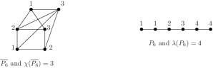
Figure 2: A graph $G$ which is a split graph but not co-linear, since $\mathcal{\chi}(G)=4$ and $\mathcal{\lambda}({\overline{G\mkern 3.0mu}\mkern-3.0mu}{})=5$.

Figure 3: Illustrating the graph ${\overline{P\mkern 3.0mu}\mkern-3.0mu}{}_{6}$ which is not a co-linear graph, since $\mathcal{\chi}({\overline{P\mkern 3.0mu}\mkern-3.0mu}{}_{6})\neq\mathcal{\lambda}(P_{6})$.

 

Although any co-linear graph is co-chordal, the reverse is not always true. For example, the graph $G$ in Figure 3 is a co-chordal graph but not a co-linear graph. Indeed, $\mathcal{\chi}(G)=4$ and $\mathcal{\lambda}({\overline{G\mkern 3.0mu}\mkern-3.0mu}{})=5$. It is easy to see that this graph is also a split graph. Moreover, the class of split graphs is distinguished from the class of co-linear graphs since the graph $C_{4}$ is a co-linear graph but not a split graph, and the graph $G$ in Figure 3 is a split graph but not a co-linear graph. However, the two classes are not disjoint; an example is the graph $C_{3}$. Recall that a graph $G$ is a split graph if there is a partition of the vertex set $V(G)=K+I$, where $K$ induces a clique in $G$ and $I$ induces an independent set; split graphs are characterized as $(2K_{2},C_{4},C_{5})$-free graphs.

We have proved that co-linear graphs are $(2K_{2},antihole)$-free. Note that, since $\overline{C_{5}}=C_{5}$ and also the chordless cycle $C_{n}$ is $2K_{2}$-free for $n\geq 6$, it is easy to see that co-linear graphs are $hole$-free. In addition, ${\overline{P\mkern 3.0mu}\mkern-3.0mu}{}_{6}$ is another forbidden induced subgraph for co-linear graphs (see Figure 3). Thus, we obtain the following result.

Proposition 3.5. If $G$ is a co-linear graph, then $G$ is $(2K_{2},antihole,{\overline{P\mkern 3.0mu}\mkern-3.0mu}{}_{6})$-free.

The forbidden graphs $2K_{2}$, $antihole$, and ${\overline{P\mkern 3.0mu}\mkern-3.0mu}{}_{6}$ are not enough to characterize completely the class of co-linear graphs, since split graphs do not contain any of these graphs as an induced subgraph. Thus, split graphs which are not co-linear graphs cannot be characterized by these forbidden induced subgraphs; see Figure 3.

4 Linear Graphs

In this section we study the complement class of co-linear graphs, namely linear graphs, in terms of forbidden induced subgraphs, and we derive inclusion relations between the class of linear graphs and other classes of perfect graphs.

4.1 Properties

We first provide a characterization of linear graphs by means of linear coloring on graphs. Since co-linear graphs are perfect, it follows that if $G$ is a co-linear graph $\chi(G_{A})=\omega(G_{A})=\alpha({\overline{G_{A}\mkern 3.0mu}\mkern-3.0mu}{})$, $\forall A\subseteq V(G)$. Therefore, the following characterization of linear graphs holds.

Proposition 4.1. A graph $G$ is linear if and only if $\mathcal{\alpha}(G_{A})=\mathcal{\lambda}(G_{A})$, $\forall A\subseteq V(G)$.

From Corollary 2.1 and Proposition 4.1 we obtain the following characterization for linear graphs.

Proposition 4.2. Linear graphs are those graphs $G$ for which the linear chromatic number achieves its theoretical lower bound in every induced subgraph of $G$.

Directly from Corollary 3.1 we can obtain the following result: any quasi-threshold graph is a linear graph. From Propositions 3.5 and 4.1 we obtain that linear graphs are $(C_{4},hole,P_{6})$-free. Therefore, the following result holds.

Proposition 4.3. Any linear graph is a chordal graph.

Although any linear graph is chordal, the reverse is not always true, i.e. not any chordal graph is a linear graph. For example, the complement ${\overline{G\mkern 3.0mu}\mkern-3.0mu}{}$ of the graph illustrated in Figure 3 is a chordal graph but not a linear graph. Indeed, $\alpha({\overline{G\mkern 3.0mu}\mkern-3.0mu}{})=4$ and $\lambda({\overline{G\mkern 3.0mu}\mkern-3.0mu}{})=5$. It is easy to see that this graph is also a split graph. Moreover, the class of split graphs is distinguished from the class of linear graphs since the graph $2K_{2}$ is a linear graph but not a split graph, and the graph ${\overline{G\mkern 3.0mu}\mkern-3.0mu}{}$ of Figure 3 is a split graph but not a linear graph. However, the two classes are not disjoint; an example is the graph $C_{3}$.

Another known subclass of the class of chordal graphs is the class of strongly chordal graphs. The following definitions and results given by Farber [12] turn up to be useful in proving some results about the structure of linear graphs. More details about strongly chordal graphs can be found in [6, 12].

   

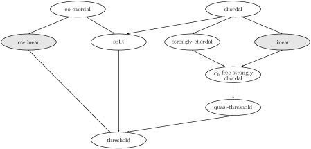
Figure 4: Illustrating the inclusion relations among the classes of linear graphs, co-linear graphs, and other classes of perfect graphs.

Definition 4.2. (Farber [12]) A vertex ordering $(v_{1},v_{2},\dots,v_{n})$ is a strong perfect elimination ordering of a graph $G$ iff $\sigma$ is a perfect elimination ordering and also has the property that for each $i$, $j$, $k$ and $\ell$, if $i<j$, $k<\ell$, $v_{k},v_{\ell}\in N[v_{i}]$, and $v_{k}\in N[v_{j}]$, then $v_{\ell}\in N[v_{j}]$. A graph is strongly chordal iff it admits a strong perfect elimination ordering.

Definition 4.3. (Farber [12]) Let $G$ be a graph. A vertex $v$ is simple in $G$ if $\{N[x]:x\in N[v]\}$ is linearly ordered by inclusion.

Theorem 4.1. (Farber [12]) A graph $G$ is strongly chordal if and only if every induced subgraph of $G$ has a simple vertex.

Corollary 4.1. (Chang [8]) A strong perfect elimination ordering of a graph $G$ is a vertex ordering $(v_{1},v_{2},\dots,v_{n})$ such that for all $i\in\{1,2,\ldots,n\}$ the vertex $v_{i}$ is simple in $G_{i}$ and also $N_{G_{i}}[v_{\ell}]\subseteq N_{G_{i}}[v_{k}]$ whenever $i\leq\ell\leq k$ and $v_{\ell},v_{k}\in N_{G_{i}}[v_{i}]$.

The following characterization of strongly chordal graphs will be next used to derive properties about the structure of linear graphs. We first give the following definition.

Definition 4.1. An incomplete $k$-sun $S_{k}$ ($k\geq 3$) is a chordal graph on $2k$ vertices whose vertex set can be partitioned into two sets, $U=\{u_{1},u_{2},\ldots,u_{k}\}$ and $W=\{w_{1},w_{2},\ldots,w_{k}\}$, so that $W$ is an independent set, and $w_{i}$ is adjacent to $u_{j}$ if and only if $i=j$ or $i=j+1$ (mod $k$). A $k$-sun is an incomplete $k$-sun $S_{k}$ in which $U$ is a complete graph.

Proposition 4.4. (Farber [12]) A chordal graph $G$ is strongly chordal if and only if it contains no induced $k$-sun.

4.2 Forbidden Subgraphs

Hereafter, we study the structure of the forbidden induced subgraphs of the class of linear graphs, and we prove that any $P_{6}$-free chordal graph which is not a linear graph properly contains a $k$-sun as an induced subgraph.

We consider the class of $P_{6}$-free chordal graphs which we have shown that it properly contains the class of linear graphs. Let $\mathcal{F}$ be the family of all the minimal forbidden induced subgraphs of the class of linear graphs. Let $F_{i}$ be a member of $\mathcal{F}$, which is neither a $C_{n}$ ($n\geq 4$) nor a $P_{6}$. We next prove the main result of this section: any graph $F_{i}$ properly contains a $k$-sun ($k\geq 3$) as an induced subgraph. From Proposition 4.4 it suffices to show that any $P_{6}$-free strongly chordal graph is a linear graph and also that the $k$-sun ($k\geq 3$) is a linear graph.

Let $G$ be a $P_{6}$-free strongly chordal graph. In order to show that $G$ is a linear graph we will show that $\alpha(G)=\lambda(G)$ and that the equality holds for every induced subgraph of $G$. Let $L$ be the set of all simple vertices of $G$, and $S$ be the set of all simplicial vertices of $G$; note that $L\subseteq S$ since a simple vertex is also a simplicial vertex. First, we construct a maximum independent set $I$ and a strong perfect elimination ordering $\sigma$ of $G$ with special properties needed for our proof. Next, we assign a coloring $\kappa:V(G)\rightarrow[k]$ to the vertices of $G$, where $k=\alpha(G)=|I|$, and show that $\kappa$ is an optimal linear coloring of $G$. Actually, we show that we can assign a linear coloring with $\lambda(G)=\alpha(G)$ colors to any $P_{6}$-free strongly chordal graph, by using the constructed strong perfect elimination ordering $\sigma$ of $G$. Finally, we show that the equality $\lambda(G_{A})=\alpha(G_{A})$ holds for every induced subgraph $G_{A}$ of $G$.

Construction of $I$ and $\sigma$. Let $G$ be a $P_{6}$-free strongly chordal graph, and let $L$ be the set of all simple vertices in $G$. From Definition 4.2, $G$ admits a strong perfect elimination ordering. Using a modified version of the algorithm given by Farber in [12] we construct a strong perfect elimination ordering $\sigma=(v_{1},v_{2},\ldots,v_{n})$ of the graph $G$ having specific properties. Our algorithm also constructs the maximum independent set $I$ of $G$. Since $G$ is a chordal graph and $\sigma$ is a perfect elimination ordering, we can use a known algorithm (e.g. see [15]) to compute a maximum independent set of the graph $G$. Throughout the algorithm, we denote by $G_{i}$ the subgraph of $G$ induced by the set of vertices $V(G)\backslash\{v_{1},v_{2},\ldots,v_{i-1}\}$, where $v_{1},v_{2},\ldots,v_{i-1}$ are the vertices which have already been added to the ordering $\sigma$ during the construction. Moreover, we denote by $I^{*}$ the set of vertices which have not been added to $\sigma$ yet and additionally do not have a neighbor already added in $\sigma$ which belongs to $I$.

In Figure 5, we present a modified version of the algorithm given by Farber [12] for constructing a strong perfect elimination ordering $\sigma$ of $G$. Our algorithm in each iteration of Steps 3–5 adds to the ordering $\sigma$ all vertices which are simple in $G_{i}$, while Farber’s algorithm selects only one simple vertex of $G_{i}$ and adds it to $\sigma$. We note that $L_{i}$ is the set of all the simple vertices of $G_{i}$ and $v_{i}$ is that vertex of $L_{i}$ which is added first to the ordering $\sigma$. It is easy to see that the constructed ordering $\sigma$ is a strong perfect elimination ordering of $G$, since every vertex which is simple in $G$ is also simple in every induced subgraph of $G$. Clearly, the constructed set $I$ is a maximum independent set of $G$.

 Input: a strongly chordal graph $G$; Output: a strong perfect elimination ordering $\sigma$ of $G$;

• set $I=\emptyset$, $I^{*}=V(G)$, $\sigma=\emptyset$, $n=|V(G)|$, and $V_{0}=V(G)$;

• Let $(V_{0},<_{0})$ be the partial ordering on $V_{0}$ in which $v<_{0}u$ if and only if $v=u$.
  set $V_{1}=V(G)$ and $i=1$;

• Let $G_{i}$ be the subgraph of $G$ induced by $V_{i}$, that is, $V_{i}=V(G_{i})$.
  construct an ordering on $V_{i}$ by $v<_{i}u$ if $v<_{i-1}u$ or $N_{i}[v]\subset N_{i}[u]$;
  set $k=i$;

• Let $L_{k}$ be the set of all the simple vertices in $G_{i}$.

  while $L_{k}\neq\emptyset$ do
  xxx$\circ$ construct an ordering on $V_{i}$ by $v<_{i}u$ if $v<_{i-1}u$ or $N_{i}[v]\subset N_{i}[u]$;
  xxx$\circ$ choose a vertex $v_{i}$ which belongs to $L_{k}$ and is minimal in $(V_{i},<_{i})$ to add to the ordering;
  xxx$\circ$ set $V_{i+1}=V_{i}\backslash\{v_{i}\}$ and $L_{k}=L_{k}\backslash\{v_{i}\}$;
  xxx$\circ$ if $v_{i}\in I^{*}$ then
  xxxxxx$\circ$ set $I=I\cup\{v_{i}\}$ and $I^{*}=I^{*}\backslash\{v_{i}\}$;
  xxxxxx$\circ$ delete all neighbors of $v_{i}$ from $I^{*}$;
  xxx$\circ$ set $i=i+1$;
  end-while;

• if  $i=n+1$   then output the ordering $\sigma=(v_{1},v_{2},\ldots,v_{n})$ of $V(G)$ and stop;
  xxxxxxxxxxxxelse go to step 3;

Figure 5: A modified version of Farber’s algorithm for constructing a strong perfect elimination ordering $\sigma$ and a maximum independent set $I$ of a strongly chordal graph $G$.

 

From the fact that $G$ is a $P_{6}$-free strongly chordal graph and from the construction of $I$ and $\sigma$ we obtain the following properties.

Property 4.1. Let $G$ be a $P_{6}$-free strongly chordal graph and let $L$ be the set of all simple vertices of $G$. For each vertex $v_{x}\notin L$, there exists a chordless path of length at most 4 connecting $v_{x}$ to any vertex $v\in L$.

Property 4.2. Let $G$ be a $P_{6}$-free strongly chordal graph, $L$ be the set of all simple vertices of $G$, and let $I$ and $\sigma$ be the maximum independent set and the ordering, respectively, constructed by our algorithm. Then,

• if $v_{i}\notin L$ and $i<j$, then $v_{j}\notin L$;

• for each vertex $v_{x}\notin I$, there exists a vertex $v_{i}\in I$, $i<x$, such that $v_{x}\in N_{G_{i}}[v_{i}]$.

Next, we describe an algorithm for assigning a coloring $\kappa$ to the vertices of $G$ using exactly $\alpha(G)$ colors and, then, we show that $\kappa$ is a linear coloring of $G$.

The coloring $\kappa$ of $G$. Let $G$ be a $P_{6}$-free strongly chordal graph, and let $L$ (resp. $S$) be the set of all simple (resp. simplicial) vertices in $G$. We consider a maximum independent set $I$, and a strong elimination ordering $\sigma$, as constructed above. Now, in order to compute the linear chromatic number $\lambda(G)$ of $G$, we assign a coloring $\kappa$ to the vertices of $G$ and show that $\kappa$ is a linear coloring of $G$. Actually, we show that we can assign a linear coloring with $\lambda(G)=\alpha(G)$ colors to any $P_{6}$-free strongly chordal graph, by using the constructed strong perfect elimination ordering $\sigma$ of $G$.

First, we assign a coloring $\kappa:V(G)\rightarrow[k]$, where $k=\alpha(G)$, to the vertices of $G$ as follows:

• Successively visit the vertices in the ordering $\sigma$ from left to right, and color the first vertex $v_{i}\in I$ which has not been assigned a color yet, with color $\kappa(v_{i})$.

• Color all uncolored vertices $v_{k}\in N_{G_{i}}(v_{i})$, with color $\kappa(v_{k})=\kappa(v_{i})$.

• Repeat steps 1 and 2 until there are no uncolored vertices $v_{i}\in I$ in $G$.

Based on this process, we obtain that every vertex $v_{i}$ belonging to the maximum independent set $I$ of $G$ is assigned a different color in step 1, and for each such vertex $v_{i}$ all its uncolored neighbors to its right in the ordering $\sigma$ are assigned the same color with $v_{i}$ in step 2. Therefore, so far we have assigned $\alpha(G)$ colors to the vertices of $G$. Now, from Property 4.2(ii) it is easy to see that $\kappa$ is a coloring of the vertex set $V(G)$, i.e. there is no vertex in $\sigma$ which has not been assigned a color. Thus, $\kappa$ is a coloring of $G$ using $\alpha(G)$ colors. Note that $\kappa$ is not a proper vertex coloring of $G$. Actually, since the following lemma holds, from Proposition 2.1 it appears that $\kappa$ is a proper vertex coloring of ${\overline{G\mkern 3.0mu}\mkern-3.0mu}{}$.

Lemma 4.1. The coloring $\kappa$ is a linear coloring of $G$.

Proof.  Let $G$ be a $P_{6}$-free strongly chordal graph, and let $L$ (resp. $S$) be the set of all simple (resp. simplicial) vertices in $G$. We consider a maximum independent set $I$, a strong elimination ordering $\sigma$, and a coloring $\kappa$ of $G$, as constructed above. Hereafter, for two vertices $v_{i}$ and $v_{j}$ in the ordering $\sigma$, we say that $v_{i}<v_{j}$ if the vertex $v_{i}$ appears before the vertex $v_{j}$ in $\sigma$.

Next, we show that $\kappa$ is a linear coloring of $G$, that is, the collection $\{\mathcal{C}_{G}(v_{\ell}):\kappa(v_{\ell})=j\}$ is linearly ordered by inclusion for all $j\in[k]$. From Corollary 2.2, it is equivalent to show that the collection $\{N_{G}[v_{\ell}]:\kappa(v_{\ell})=j\}$ is linearly ordered by inclusion for all $j\in[k]$. Each such collection contains exactly one set $N_{G}[v_{i}]$ where $v_{i}\in I$, and some sets $N_{G}[v_{k}]$ where $v_{k}$ are neighbors of $v_{i}$ in $G_{i}$ and $\kappa(v_{k})=\kappa(v_{i})$. Thus, it suffices to show that for each vertex $v_{i}\in I$, the collection $\{N_{G}[v_{k}]:v_{k}\in N_{G_{i}}[v_{i}]\ and\ \kappa(v_{k})=\kappa(v_{i})\}$ is linearly ordered by inclusion. To this end, we distinguish two cases regarding the vertices $v_{i}\in I$; in the first case we consider $v_{i}$ to be a simplicial vertex, that is $v_{i}\in S$, and in the second case we consider $v_{i}\notin S$.

Case 1: The vertex $v_{i}\in I$ and $v_{i}\in S$. Since $\sigma$ is a strong elimination ordering, each vertex $v_{i}\in I$ is simple in $G_{i}$ and thus $\{N_{G_{i}}[v_{k}]:v_{k}\in N_{G_{i}}[v_{i}]\}$ is linearly ordered by inclusion. We will show that $\{N_{G}[v_{k}]:v_{k}\in N_{G_{i}}[v_{i}]\ and\ \kappa(v_{k})=\kappa(v_{i})\}$ is linearly ordered by inclusion for all vertices $v_{i}\in I\cap S$. Recall that in the coloring $\kappa$ of $G$ we assign the color $\kappa(v_{k})=\kappa(v_{i})$ to a vertex $v_{k}\notin I$, if $v_{i}\in I$, $v_{k}\in N_{G_{i}}[v_{i}]$ and there exists no vertex $v_{i^{\prime}}\in I$ such that $v_{k}\in N_{G_{i^{\prime}}}[v_{i^{\prime}}]$ and $v_{i}^{\prime}<v_{i}$ in $\sigma$. By definition, if $v_{i}\in L$ then the collection $\{N_{G}[v_{k}]:v_{k}\in N_{G_{i}}[v_{i}]\ and\ \kappa(v_{k})=\kappa(v_{i})\}$ is linearly ordered by inclusion. Thus, hereafter we consider vertices $v_{i}\in I\cap S$ and $v_{i}\notin L$.

Consider that the vertex $v_{i}$ has a neighbor $v_{1}$ to its left in the ordering $\sigma$, i.e. $v_{1}<v_{i}$. Since $v_{i}$ is a simplicial vertex in $G$, its closed neighborhood forms a clique and, thus, $v_{1}\in N_{G}[v_{k}]$ for all vertices $v_{k}\in N_{G_{i}}[v_{i}]$. Therefore, the existence of such a vertex $v_{1}$ preserves the linear order by inclusion of $\{N_{G_{i}}[v_{k}]\cup\{v_{1}\}:v_{k}\in N_{G_{i}}[v_{i}]\}$. Thus, $N_{G}[v_{i}]\subseteq N_{G}[v_{k}]$, for all vertices $v_{k}\in N_{G_{i}}[v_{i}]$ and $\kappa(v_{k})=\kappa(v_{i})$.

Now, consider that the vertex $v_{i}$ has two neighbors $v_{k}$ and $v_{j}$ to its right in the ordering $\sigma$, such that $v_{i}<v_{k}<v_{j}$ and $\kappa(v_{k})=\kappa(v_{j})=\kappa(v_{i})$; thus, $N_{G_{i}}[v_{k}]\subseteq N_{G_{i}}[v_{j}]$. In the case where the equality $N_{G_{i}}[v_{k}]=N_{G_{i}}[v_{j}]$ holds, without loss of generality, we may assume that the degree of $v_{k}$ in $G$ is less than or equal to the degree of $v_{j}$ in $G$ (note that $\sigma$ is still a strong elimination ordering). Assume that $N_{G}[v_{k}]\subseteq N_{G}[v_{j}]$ does not hold. Then, there exist vertices $v_{2}$ and $v_{3}$ in $G$ such that $v_{2}\in N_{G}[v_{k}]$, $v_{2}\notin N_{G}[v_{j}]$, $v_{3}\in N_{G}[v_{j}]$, and $v_{3}\notin N_{G}[v_{k}]$. Since $N_{G_{i}}[v_{k}]\subseteq N_{G_{i}}[v_{j}]$, it is easy to see that $v_{2}<v_{i}$ in $\sigma$. Assume that $v_{2}$ is the first (from left to right) neighbor of $v_{k}$ in $\sigma$. Since $\kappa(v_{k})=\kappa(v_{i})$, it follows that $v_{2}\notin I$. Moreover, from Property 4.2(ii) it holds that there exists a vertex $v_{4}\in I$, such that $v_{4}<v_{2}$ and $v_{2}\in N_{G}[v_{4}]$. Additionally, since $\kappa(v_{k})=\kappa(v_{j})=\kappa(v_{i})$ it holds that $v_{k},v_{j}\notin N_{G}[v_{4}]$. Hence, the subgraph of $G$ induced by the vertices $\{v_{4},v_{2},v_{k},v_{j}\}$ is a $P_{4}$. Concerning now the position of the vertex $v_{3}$ in the ordering $\sigma$, we can have either $v_{3}<v_{i}$ in the case where $N_{G_{i}}[v_{k}]=N_{G_{i}}[v_{j}]$ holds, or $v_{3}>v_{i}$ otherwise. We will show that in both cases we are leaded to a contradiction to our initial assumptions; that is, either it results that $G$ has a $P_{6}$ as an induced subgraph or that the vertices should be added to $\sigma$ in an order different to the one originally assumed.

Case 1.1. $v_{3}<v_{i}$. It is easy to see that $v_{3}\notin I$, since otherwise $v_{j}$ would have taken the color $\kappa(v_{j})=\kappa(v_{3})$ during the coloring $\kappa$ of $G$. Thus, from Property 4.2(ii) there exists a vertex $v_{5}\in I$, such that $v_{5}<v_{3}$ and $v_{3}\in N_{G}[v_{5}]$. Therefore, the vertices $\{v_{4},v_{2},v_{k},v_{j},v_{3},v_{5}\}$ induce a $P_{6}$ in $G$, which is also chordless since $G$ is chordal.

Case 1.2. $v_{3}>v_{i}$. Since $v_{i}\notin L$, from Property 4.2(i) it follows that $v_{3}\notin L$. Thus, from Property 4.1 we obtain that there exists a chordless path of length at most 4 connecting $v_{3}\notin L$ to any vertex $v\in L$. Similarly, it easily follows that $v_{4}\in L$. However, we know that in a non-trivial strongly chordal graph there exist at least two non adjacent simple vertices [12]. Thus, there exist a vertex $v\in L$, $v\neq v_{4}$, such that the distance $d(v,v_{3})$ of $v_{3}$ from $v$ is at most 4. Let $d_{m}(v_{3},v)=max\{d(v_{3},v):\ \forall v\in L,\ v\neq v_{4}\}$. Since $v_{3}\notin L$ and $G$ is $P_{6}$-free, it follows that $1\leq d_{m}(v,v_{3})\leq 4$.

Next, we distinguish four cases regarding the maximum distance $d_{m}(v_{3},v)$ and show that each one comes to a contradiction. In each case we have that $\{v_{4},v_{2},v_{k},v_{j},v_{3}\}$ is a chordless path on five vertices. We first explain what is illustrated in Figures 6 and  7. Let $G_{y}$ be the induced subgraph of $G$, such that during the construction of $\sigma$ the vertex $v_{i}$ is simple in $G_{y}$, i.e. $v_{i}\in L_{y}$ and $v_{y}\leq v_{i}$. In the two figures, the vertices are placed on the horizontal dotted line in the order that appear in the ordering $\sigma$. For the vertices which are not placed on the dotted line, we are only interested about illustrating the edges among them. The vertices which are to the right of the vertical dashed line belong to the induced subgraph $G_{y}$ of $G$. The dashed edges illustrate edges that may or may not exist in the specific case. Next, we distinguish the four cases, and show that each one of them comes to a contradiction:

 

Figure 6: Illustrating Case (A) and Case (B.a)

 

• Case (A): $d_{m}(v_{3},v)=1$. It is easy to see that $v_{j}v\notin E(G)$, since otherwise $v_{j}$ would have been assigned the color $\kappa(v)$ and not $\kappa(v_{i})$ as assumed. Thus, in this case there exists a $P_{6}$ in $G$ induced by the vertices $\{v_{4},v_{2},v_{k},v_{j},v_{3},v\}$; since $G$ is a chordal graph, other edges among the vertices of this path do not exist. This is a contradiction to our assumption that $G$ is a $P_{6}$-free graph.

• Case (B): $d_{m}(v_{3},v)=2$. In this case there exists a vertex $v_{5}$ such that $\{v_{3},v_{5},v\}$ is a chordless path from $v_{3}$ to $v$. It follows that there exists a $P_{7}$ induced by the vertices $\{v_{4},v_{2},v_{k},v_{j},v_{3},v_{5},v\}$. Having assumed that $G$ is a $P_{6}$-free graph, the path $\{v_{4},v_{2},v_{k},v_{j},v_{3}\}$ is chordless and $v_{j},v_{k}\notin N_{G}[v]$, we obtain that $v_{j}v_{5}\in E(G)$ and $v_{k}v_{5}\in E(G)$. Next, we distinguish three cases regarding the neighborhood of the vertex $v_{3}$ in $G$ and show that each one comes to a contradiction.

  • The vertex $v_{3}$ does not have neighbors in $G$ other than $v_{5}$ and $v_{j}$. In Case (i) we examine the cases where either $v_{2}v_{5}\notin E(G)$ or $v_{2}v_{5}\in E(G)$ and $v_{j}$ does not have a neighbor $v_{x}$ in $G_{i}$, such that $v_{x}v_{k}\notin E(G)$. In Case (ii) we examine the case where $v_{2}v_{5}\in E(G)$ and $v_{j}$ has a neighbor $v_{x}$ in $G_{i}$, such that $v_{x}v_{k}\notin E(G)$.

    • Assume that $v_{2}v_{5}\notin E(G)$. In this case, we can see that during the construction of $\sigma$, after the first iteration where $v$ and $v_{4}$ are added in the ordering, the vertex $v_{3}$ becomes simple in the remaining induced subgraph of $G$, since $N[v_{5}]$ becomes a subset of $N[v_{j}]$. Thus, $v_{3}$ can be added to $\sigma$ during the second iteration of the algorithm, along with $v_{2}$. However, $v_{i}$ will not be added to the ordering before the third iteration, since $v_{i}$ is not simple before $v_{2}$ is added to $\sigma$. Thus, we conclude that $v_{3}$ will be added in $\sigma$ before $v_{i}$, and more specifically that $v_{3}<v_{y}\leq v_{i}$, and this is a contradiction to our assumption that $v_{3}>v_{i}$.

      Now, assume that $v_{2}v_{5}\in E(G)$. We know that $v_{2}$ is simple in the subgraph $G_{2}$ of $G$ induced by the vertices to the right of $v_{2}$ in $\sigma$. If $v_{5},v_{k}\in N_{G_{2}}[v_{2}]$, $v_{3}\in N_{G_{2}}[v_{5}]$, and $v_{3}\notin N_{G_{2}}[v_{k}]$, then $N_{G_{2}}[v_{5}]\supset N_{G_{2}}[v_{k}]$. More specifically, since we have assumed that $v_{2}$ is the first (from left to right) neighbor of $v_{k}$ in $\sigma$, it follows that $N_{G}[v_{5}]\supset N_{G}[v_{k}]$. We know that $N_{G_{i}}[v_{k}]\subset N_{G_{i}}[v_{j}]$, and since we have assumed that $v_{j}$ does not have a neighbor $v_{x}$, such that $v_{x}<v_{i}$, it easily follows that $N_{G_{i}}[v_{k}]\subset N_{G_{i}}[v_{j}]=N_{G}[v_{j}]$. Thus, for every neighbor of $v_{j}$ in $G$, which is also a neighbor of $v_{k}$, we obtain that it is a neighbor of $v_{5}$ as well.

      Therefore, in the case where $v_{j}$ does not have a neighbor $v_{x}$ in $G$, and thus in $G_{i}$, such that $v_{x}v_{k}\notin E(G)$, it follows that $N_{G}[v_{5}]$ is a superset of $N_{G}[v_{j}]$ and, thus, the vertex $v_{3}$ is simple in $G$. Again we conclude that $v_{3}$ will be added to $\sigma$ before $v_{i}$, and more specifically that $v_{3}<v_{y}\leq v_{i}$. This is a contradiction to our assumption that $v_{3}>v_{i}$.

    • Consider now the case where $v_{2}v_{5}\in E(G)$ and $v_{j}$ has a neighbor $v_{x}$ in $G$, and thus in $G_{i}$, such that $v_{x}v_{k}\notin E(G)$. We will show that in this case either $v_{3}$ is simple after the first iteration, i.e. $v_{x}\in N[v_{5}]$ or $v_{x}$ becomes simple after the first iteration. Since $v_{x}>v_{i}$ it follows that $v_{x}\notin L$. Therefore, there exists a path in $G$ from $v_{x}$ to a vertex $v^{\prime}\in L$ of length $d(v_{x},v^{\prime})$ at most 4. Consider the case where $d(v_{x},v^{\prime})=1$. If $v\equiv v^{\prime}$, then $v_{5}v_{x}\in E(G)$, since $G$ is a chordal graph; thus, $N[v_{5}]\supseteq N[v_{j}]$ and $v_{3}\in L$. It is easy to see that $v^{\prime}\neq v_{4}$, since $G$ is a chordal graph. Therefore, in the case where $v^{\prime}v_{x}\in E(G)$, the graph $G$ has a $P_{6}$ induced by the vertices $\{v_{4},v_{2},v_{k},v_{j},v_{x},v^{\prime}\}$. Thus, $v^{\prime}v_{x}\notin E(G)$ and there exists a vertex $v_{z}$ such that $\{v_{x},v_{z},v^{\prime}\}$ is a chordless path from $v_{x}$ to $v^{\prime}$. Therefore, there exists a $P_{7}$ in $G$ and, thus, $v_{k},v_{j}\in N_{G}[v_{z}]$. Additionally, from Case(B.a)(i) we have that $v_{5}\in N_{G}[v_{z}]$ (recall that if $v_{2}v_{5}\in E(G)$, then $N_{G}[v_{5}]\supset N_{G}[v_{k}]$).

      Note that, the vertices $v_{x}$ and $v_{z}$ play the same role in $G$ as the vertices $v_{3}$ and $v_{5}$, respectively. Therefore, in the case where $v_{2}v_{z}\notin E(G)$, the vertex $v_{x}$ is simple after the first iteration and will be added to $\sigma$ during the second iteration, while $v_{i}$ will be added during the third. Thus, we will have $v_{x}<v_{y}<v_{i}$ which is a contradiction to our assumption that $v_{x}>v_{i}$. Consider now the case where $v_{2}v_{z}\in E(G)$. Since $v_{2}$ is simple in the subgraph $G_{2}$ of $G$ induced by the vertices to the right of $v_{2}$ in $\sigma$, we must have either $v_{z}v_{3}\in E(G)$ or $v_{5}v_{x}\in E(G)$. Without loss of generality assume that $v_{5}v_{x}\in E(G)$. Concluding, we have shown that even in the case where $v_{j}$ has a neighbor $v_{x}$ in $G$, and thus in $G_{i}$, such that $v_{x}v_{k}\notin E(G)$, then $N_{G}[v_{5}]$ is a superset of $N_{G}[v_{j}]$, and thus $v_{3}\in L$. Thus, we have again $v_{3}<v_{y}<v_{i}$ which is a contradiction to our assumption that $v_{3}>v_{i}$. The same holds even if, additionally to the other edges, $v_{4}v_{5}\in E(G)$.

  So far, we have shown that if $v_{3}$ has the vertices $v_{j}$ and $v_{5}$ as neighbors, then either $v_{3}\in L$ or $v_{3}$ is simple in the second iteration, that is before $v_{i}$ can be added to $\sigma$ (i.e. $v_{3}<v_{y}\leq v_{i}$). This is due to the fact that for any neighbor $v_{5}$ of $v_{3}$ we have shown that $N[v_{5}]\subseteq N[v_{j}]$ in the case where $v_{2}v_{5}\notin E(G)$, and $N[v_{5}]\supseteq N[v_{j}]$ in the case where $v_{2}v_{5}\in E(G)$; thus $v_{3}$ will be added to $\sigma$ before $v_{i}$. Since we initially assumed that $v_{3}>v_{i}$ in $\sigma$, i.e. that $v_{3}$ does not become simple before $v_{i}$ becomes simple, we continue by examining the cases where $v_{3}$ has neighbors in $G_{y}$ other than $v_{5}$ and $v_{j}$.

  • The vertex $v_{3}$ has two neighbors $v_{5}$ and $v_{5}^{\prime}$ in $G_{y}$, such that $v_{5}v_{5}^{\prime}\notin E(G)$. Since we have assumed that the maximum distance of the vertex $v_{3}$ from $v$ in $G$, for any vertex $v\in L$, $v\neq v_{4}$, is $d_{m}(v_{3},v)=2$, and $v_{3}$ has no neighbor belonging to $L$, it follows that $v_{5},v_{5}^{\prime}\notin L$ and there exist vertices $v,v^{\prime}\in L$ such that the vertices $\{v_{3},v_{5},v\}$ induce a chordless path from $v_{3}$ to $v$ and $\{v_{3},v_{5}^{\prime},v^{\prime}\}$ induce a chordless path from $v_{3}$ to $v^{\prime}$. It is easy to see that $v\neq v^{\prime}$ and $vv^{\prime}\notin E(G)$ since $G$ is a chordal graph. Therefore, from Case (B.a) we have $v_{k},v_{j}\in N_{G}[v_{5}]$ and $v_{k},v_{j}\in N_{G}[v_{5}^{\prime}]$. However, in this case there exists a $C_{4}$ in $G$ induced by the vertices $\{v_{5},v_{3},v_{5}^{\prime},v_{k}\}$, since by assumption $v_{5}v_{5}^{\prime}\notin E(G)$ and $v_{3}v_{k}\notin E(G)$. It easily follows that the same arguments hold for any two neighbors of $v_{3}$ in $G$. Concluding, the vertex $v_{3}$ cannot have two neighbors $v_{5}$ and $v_{5}^{\prime}$ in $G$, such that $v_{5}v_{5}^{\prime}\notin E(G)$. Thus, $v_{3}\in S$.

       

    Figure 7: Illustrating Cases (B.b) and (B.c) of the proof.

  • The vertex $v_{3}$ has two neighbors $v_{5}$ and $v_{5}^{\prime}$ (where $v_{5}\neq v_{j}$ and $v_{5}^{\prime}\neq v_{j}$) in $G_{y}$, such that $v_{5}v_{5}^{\prime}\in E(G)$, but neither $N_{y}[v_{5}]\subseteq N_{y}[v_{5}^{\prime}]$ nor $N_{y}[v_{5}^{\prime}]\subseteq N_{y}[v_{5}]$; thus, there exist vertices $v_{6}$ and $v_{6}^{\prime}$ in $G_{y}$ such that $v_{5}v_{6}\in E(G)$ and $v_{5}v_{6}^{\prime}\notin E(G)$ and, also, $v_{5}^{\prime}v_{6}^{\prime}\in E(G)$ and $v_{5}^{\prime}v_{6}\notin E(G)$. Since $v_{3}\in S$, it follows that $v_{6},v_{6}^{\prime}\notin N_{G}[v_{3}]$. Since $d_{m}(v_{3},v)=2$, there exists a vertex $v\in L$ such that $\{v_{3},v_{5},v\}$ is a chordless path from $v_{3}$ to $v$. Similarly, there exists a vertex $v^{\prime}\in L$ such that $\{v_{3},v_{5},v^{\prime}\}$ is a chordless path from $v_{3}$ to $v^{\prime}$. We have that $v\neq v^{\prime}$, $vv_{5}^{\prime}\notin E(G)$ and $v^{\prime}v_{5}\notin E(G)$, since otherwise $v$ and $v^{\prime}$ would not be simple in $G$. Additionally, $vv^{\prime}\notin E(G)$, $vv_{6}^{\prime}\notin E(G)$, and $v^{\prime}v_{6}\notin E(G)$, since $G$ is a chordal graph. Therefore, from Case (B.a) we have $v_{k},v_{j}\in N_{G}[v_{5}]$ and $v_{k},v_{j}\in N_{G}[v_{5}^{\prime}]$. Assume that there exist vertices $v^{\prime\prime},v^{\prime\prime\prime}\in L$, such that $v_{6}v^{\prime\prime\prime}\in E(G)$ and $v_{6}^{\prime}v^{\prime\prime}\in E(G)$. It is easy to see that at least one of the equivalences $v\equiv v^{\prime\prime\prime}$ and $v^{\prime}\equiv v^{\prime\prime}$ holds, otherwise $G$ has a $P_{6}$ induced by the vertices $\{v^{\prime\prime\prime},v_{6},v_{5},v_{5}^{\prime},v_{6}^{\prime},v^{\prime\prime}\}$. Without loss of generality, assume that $v\equiv v^{\prime\prime\prime}$ holds.

    Since $v\in L$, $v_{5},v_{6}\in N_{G}[v]$, $v_{5}^{\prime}\in N_{G}[v_{5}]$, and $v_{5}^{\prime}\notin N_{G}[v_{6}]$, it follows that $N_{G}[v_{6}]\subset N_{G}[v_{5}]$. In the case where $v_{k},v_{j}\notin N_{G}[v_{6}]$ we have $v_{6}\in L$ and, thus, $v_{6}$ would be added to $\sigma$ in the first iteration which is a contradiction to our assumption that $v_{6}\in G_{y}$. Assume that $v_{j}v_{6}\in E(G)$; it follows that $v_{k}v_{6}\in E(G)$, since otherwise $G$ has a $P_{6}$ induced by the vertices $\{v_{4},v_{2},v_{k},v_{j},v_{6},v\}$. If $v^{\prime}\equiv v^{\prime\prime}$, the same arguments hold for $v_{6}^{\prime}$ too and, thus, if $v_{j}v_{6}^{\prime}\in E(G)$ then $v_{k}v_{6}^{\prime}\in E(G)$. In the case where $v^{\prime}\neq v^{\prime\prime}$ we have $v_{6}^{\prime}v_{k}\in E(G)$, since otherwise $G$ has a $P_{6}$ induced by the vertices $\{v_{4},v_{2},v_{k},v_{5}^{\prime},v_{6}^{\prime},v^{\prime\prime}\}$. Thus, in any case $v_{6},v_{6}^{\prime}\in N_{G}[v_{k}]$, and $G$ has a $3$-sun induced by the vertices $\{v_{k},v_{5},v_{5}^{\prime},v_{6}^{\prime},v_{6},v_{3}\}$. Since other edges between the vertices of the $3$-sun do not exist, it follows that at least one of the vertices $v_{6}$ and $v_{6}^{\prime}$ does not belong to the neighborhood of $v_{k}$ and, thus, of $v_{j}$ in $G$. Without loss of generality, let $v_{6}$ be that vertex. Thus, $v_{6}\in L$ and, subsequently, $v_{6}$ will be added to $\sigma$ during the first iteration. Thus, $v_{3}$ is simple and will be added to $\sigma$ during the second iteration, along with $v_{2}$, while $v_{i}$ will be added to $\sigma$ after the second iteration (i.e. $v_{3}<v_{y}\leq v_{i}$). This is a contradiction to our assumption that $v_{3}>v_{i}$.

    Using similar arguments, we can prove that $v_{3}$ will be added to $\sigma$ before $v_{i}$, even if there exist edges between $v_{2}$ and the vertices $v_{5}$, $v_{5}^{\prime}$, $v_{6}$, and $v_{6}^{\prime}$. Actually, it easily follows that $v_{2}v_{6}\notin E(G)$, since $v_{6}v_{k}\notin E(G)$ and $G$ is a chordal graph. Additionally, $v_{2}v_{5}\notin E(G)$, since we know that $v_{5}v_{6}^{\prime}\notin E(G)$, $v_{k}v_{3}\notin E(G)$ and $v_{2}$ is simple in $G_{2}$. Therefore, whether $v_{2}v_{5}^{\prime},v_{2}v_{6}^{\prime}\in E(G)$ or not, it does not change the fact that $v_{3}$ becomes simple after the first iteration and, thus, $v_{3}$ is added to $\sigma$ before $v_{i}$. Note, that even in the case where $v\equiv v_{4}$ or $v^{\prime}\equiv v_{4}$, it similarly follows that $v_{6}^{\prime}\in L$ or $v_{6}\in L$ respectively and, thus, $v_{3}$ becomes simple after the first iteration and is added to $\sigma$ before $v_{i}$.

• Case (C): $d_{m}(v_{3},v)=3$. In this case there exist vertices $v_{5}$ and $v_{6}$ such that $\{v_{3},v_{5},v_{6},v\}$ is a chordless path from $v_{3}$ to $v$. Since now $G$ has a $P_{8}$, it follows that $v_{5}v_{j}\in E(G)$ and, additionally, some other edges must exist among the vertices $v_{2}$, $v_{k}$, $v_{j}$, $v_{5}$, and $v_{6}$. In any case, we will prove that either $N_{G}[v_{5}]\subseteq N_{G}[v_{j}]$ or $N_{G}[v_{j}]\subseteq N_{G}[v_{5}]$ and, thus, $v_{3}\in L$. Similarly to Case (B), we distinguish three cases regarding the neighborhood of the vertex $v_{3}$ in $G$ and show that if $v_{3}\notin L$ then each one comes to a contradiction.

  • The vertex $v_{3}$ does not have neighbors in $G$ other than $v_{5}$ and $v_{j}$. Consider the case where $v_{3}\notin L$ because $v_{6}\notin N_{G}[v_{j}]$ and $v_{k}\notin N_{G}[v_{5}]$. In this case, $G$ has a $P_{7}$ induced by the vertices $\{v_{4},v_{2},v_{k},v_{j},v_{5},v_{6},v\}$ which is chordless since $G$ is a chordal graph; this is a contradiction to our assumption that $G$ is $P_{6}$-free. Consider, now, the case where $v_{3}\notin L$ because $v_{6}\notin N_{G}[v_{j}]$ and $v_{i}\notin N_{G}[v_{5}]$. Since $G$ is $P_{6}$-free it follows that $v_{5}v_{k}\in E(G)$ and $v_{6}v_{k}\in E(G)$. However, in this case $G$ has a $3$-sun, unless either $v_{i}v_{6}\in E(G)$ and, thus, $v_{j}v_{6}\in E(G)$, or $v_{i}v_{5}\in E(G)$. In either case it follows that $v_{3}\in L$.

    Consider, now, the case where $v_{j}$ has another neighbor $v_{x}$ in $G_{i}$ such that $v_{x}v_{5}\notin E(G)$. Using similar arguments as in Case (B.a)(ii), we come to a contradiction to our assumptions. More specifically, in the case where $v_{2}v_{5}\in E(G)$, it is proved that $N_{G}[v_{5}]\supset N_{G}[v_{j}]$, and thus $v_{3}\in L$. Similarly, in the case where $v_{6}v_{j}\notin E(G)$, it is proved that the vertex $v_{x}$ will be simple after the first iteration during the construction of $\sigma$, and thus $v_{x}<v_{y}\leq v_{i}$.

  • The vertex $v_{3}$ has two neighbors $v_{5}$ and $v_{5}^{\prime}$ in $G_{y}$, such that $v_{5}v_{5}^{\prime}\notin E(G)$. Using the same arguments as in Case (B.b), we obtain that in this case $G$ has a $C_{4}$ which is a contradiction to our assumptions.

  • The vertex $v_{3}$ has two neighbors $v_{5}$ and $v_{5}^{\prime}$ (where $v_{5}\neq v_{j}$ and $v_{5}^{\prime}\neq v_{j}$) in $G_{y}$, such that $v_{5}v_{5}^{\prime}\in E(G)$, and neither $N_{y}[v_{5}]\subseteq N_{y}[v_{5}^{\prime}]$ nor $N_{y}[v_{5}^{\prime}]\subseteq N_{y}[v_{5}]$; that is, there exist vertices $v_{6}$ and $v_{6}^{\prime}$ in $G_{y}$ such that $v_{5}v_{6}\in E(G)$ and $v_{5}v_{6}^{\prime}\notin E(G)$ and, also, $v_{5}^{\prime}v_{6}^{\prime}\in E(G)$ and $v_{5}^{\prime}v_{6}\notin E(G)$. Similarly to Case (B.c), we can prove that this case comes to a contradiction as well. Note that, in this case $d_{m}(v_{3},v)=3$ and, thus, there exists a chordless path $\{v_{3},v_{5},v_{7},v\}$ from $v_{3}$ to $v$. Again, at least one of $v\equiv v^{\prime\prime\prime}$ and $v^{\prime}\equiv v^{\prime\prime}$ must hold, since otherwise $G$ has a $P_{6}$ induced by the vertices $\{v^{\prime\prime\prime},v_{6},v_{5},v_{5}^{\prime},v_{6}^{\prime},v^{\prime\prime}\}$. Using the same arguments as in Case (B.c), we obtain that if $v\equiv v^{\prime\prime\prime}$ then $v_{k},v_{j}\notin N_{G}[v_{6}]$. However, now, we must additionally have $v_{6}v_{7}\in E(G)$, since otherwise $G$ has a $C_{4}$ induced by the vertices $\{v,v_{7},v_{5},v_{6}\}$. Therefore, as in Case (B.c) we obtain $v_{6}\in L$, which is a contradiction to our assumption that the vertex $v_{i}$ appears in the ordering before the vertices $v_{6}$, $v_{6}^{\prime}$, $v_{5}$, and $v_{5}^{\prime}$.

• Case (D): $d_{m}(v_{3},v)=4$. In this case there exist vertices $v_{5}$, $v_{6}$ and $v_{7}$ such that $\{v_{3},v_{5},v_{6},v_{7},v\}$ is a chordless path from $v_{3}$ to $v$. Since now $G$ has a $P_{9}$, it follows that $v_{5}v_{j}\in E(G)$ and, additionally, some other edges must exist. Similarly to Cases (A) and (B), we distinguish three cases regarding the neighborhood of the vertex $v_{3}$ in $G$ and show that if $v_{3}\notin L$ then each one comes to a contradiction.

  • The $v_{3}$ does not have neighbors in $G$ other than $v_{5}$ and $v_{j}$. If we assume that $v_{3}\notin L$, then $v_{5}$ has a neighbor in $G$ which is not a neighbor of $v_{j}$ and, additionally, $v_{j}$ has a neighbor in $G$ which is not a neighbor of $v_{5}$. Thus, we can have one of the following three cases, each of which comes to a contradiction:

    • $v_{2}\in N_{G}[v_{5}]$ and $v_{7}\in N_{G}[v_{j}]$. Now, we have that $v_{2}v_{6}\in E(G)$, since otherwise $G$ has a $P_{6}$ induced by the vertices $\{v_{4},v_{2},v_{5},v_{6},v_{7},v\}$. However, in this case $v_{2}$ would not be simple in $G_{2}$, where $G_{2}$ is the subgraph of $G$ induced by the vertices to the right of $v_{2}$ in $\sigma$, since $v_{7}\in N_{G}[v_{6}]$ and $v_{7}\notin N_{G}[v_{5}]$ and, also, $v_{3}\in N_{G}[v_{5}]$ and $v_{3}\notin N_{G}[v_{6}]$. Indeed, it suffices to show that the vertices $v_{5}$, $v_{6}$, $v_{7}$, and $v_{3}$ belong to the induced subgraph $G_{2}$ of $G$.

      We know that $v_{5},v_{3}\in N_{G}[v_{j}]$ and, thus, $v_{5}>v_{i}$ and $v_{3}>v_{i}$ since we have assumed that $v_{j}$ does not have a neighbor $v_{x}$, such that $v_{x}<v_{i}$. Additionally, from $v_{7}\in N_{G}[v_{j}]$ it follows that $v_{6}\in N_{G}[v_{j}]$, since otherwise $G$ has a $C_{4}$ induced by the vertices $\{v_{j},v_{5},v_{6},v_{7}\}$. Therefore, $v_{6},v_{7}\in N_{G}[v_{j}]$ and, thus, $v_{i}<v_{6}$ and $v_{i}<v_{7}$. Therefore, the vertices $v_{5}$, $v_{6}$, $v_{7}$, and $v_{3}$ belong to the induced subgraph $G_{2}$ of $G$, and thus, the vertex $v_{2}$ is not simple in $G_{2}$, which is a contradiction to our assumption that $\sigma$ is a strong perfect elimination ordering.

    • $v_{k}\notin N_{G}[v_{5}]$ and $v_{6}\notin N_{G}[v_{j}]$. From $v_{k}\notin N_{G}[v_{5}]$ we obtain that $v_{2},v_{i}\notin N_{G}[v_{5}]$. In this case $G$ has a $P_{8}$ induced by the vertices $\{v_{4},v_{2},v_{k},v_{j},v_{5},v_{6},v_{7},v\}$. This path is chordless since $G$ is a chordal graph.

    • $v_{i}\notin N_{G}[v_{5}]$ and $v_{6}\notin N_{G}[v_{j}]$. In this case, we have a $P_{8}$ in $G$ induced by the vertices $\{v_{4},v_{2},v_{k},v_{j},v_{5},v_{6},v_{7},v\}$; thus, $v_{k}v_{5}\in E(G)$. From $v_{i}\notin N_{G}[v_{5}]$ we obtain that $v_{2}\notin N_{G}[v_{5}]$ and, thus, $v_{6}v_{k}\in E(G)$. Now, $G$ has a $3$-sun induced by the vertices $\{v_{5},v_{k},v_{j},v_{6},v_{i},v_{3}\}$, since we have assumed that $v_{i}v_{5}\notin E(G)$, $v_{6}v_{j}\notin E(G)$, and other edges do not exist by assumption. This is a contradiction to our assumption that $G$ is a strongly chordal graph.

    Using similar arguments as in Case (B.a)(ii) and Case (C.a), we can prove that if $v_{3}\notin L$ we come to a contradiction, even in the case where $v_{j}$ has another neighbor $v_{x}$ in $G_{i}$ such that $v_{x}v_{5}\notin E(G)$. Indeed, in the case where $v_{2}v_{5}\in E(G)$ we can prove that $N_{G}[v_{5}]\supset N_{G}[v_{j}]$ and, thus, $v_{3}\in L$. In the case where $v_{6}v_{j}\notin E(G)$, the vertex $v_{x}$ will be simple after the first iteration during the construction of $\sigma$ and, thus, $v_{x}<v_{y}\leq v_{i}$.

  • The vertex $v_{3}$ has two neighbors $v_{5}$ and $v_{5}^{\prime}$ in $G_{y}$, such that $v_{5}v_{5}^{\prime}\notin E(G)$. Using the same arguments as in Case (B.b), we obtain that in this case $G$ has a $C_{4}$ which is a contradiction to our assumptions.

  • The vertex $v_{3}$ has two neighbors $v_{5}$ and $v_{5}^{\prime}$ (where $v_{5}\neq v_{j}$ and $v_{5}^{\prime}\neq v_{j}$) in $G_{y}$, such that $v_{5}v_{5}^{\prime}\in E(G)$, and neither $N_{y}[v_{5}]\subseteq N_{y}[v_{5}^{\prime}]$ nor $N_{y}[v_{5}^{\prime}]\subseteq N_{y}[v_{5}]$. Using the same arguments as in Cases (B.c) and (C.c), we can prove that this case comes to a contradiction.

Case 2: The vertex $v_{i}\in I$ and $v_{i}\notin S$. Since $\sigma$ is a strong perfect elimination ordering, each vertex $v_{i}\in I$ is simple in $G_{i}$ and, thus, $\{N_{G_{i}}[v_{k}]:v_{k}\in N_{G_{i}}[v_{i}]\}$ is linearly ordered by inclusion. We will show that $\{N_{G}[v_{k}]:v_{k}\in N_{G_{i}}[v_{i}]\ and\ \kappa(v_{k})=\kappa(v_{i})\}$ is linearly ordered by inclusion for all vertices $v_{i}\in I$ and $v_{i}\notin S$. Since $v_{i}$ is not a simplicial vertex in $G$, there exist at least two vertices $v_{2}^{\prime},v_{j}^{\prime}\in N_{G}(v_{i})$ such that $v_{2}^{\prime}v_{j}^{\prime}\notin E(G)$. In the case where there exist no neighbors $v_{2}^{\prime}$ and $v_{j}^{\prime}$ of $v_{i}$, such that $v_{2}^{\prime}<v_{i}<v_{j}^{\prime}$ and $v_{2}^{\prime}v_{j}^{\prime}\notin E(G)$, we have exactly the same situation as in Case 1, where every neighbor $v_{j}^{\prime}$ of $v_{i}$ in $G_{i}$ was joined by an edge with every neighbor $v_{2}^{\prime}$ of $v_{i}$, such that $v_{2}^{\prime}<v_{i}<v_{j}^{\prime}$. Let us now consider the case where $v_{i}$ has two neighbors $v_{2}^{\prime}$ and $v_{j}^{\prime}$, such that $v_{2}^{\prime}<v_{i}<v_{j}^{\prime}$ and $v_{2}^{\prime}v_{j}^{\prime}\notin E(G)$.

Using the same arguments as in Case 1 we can prove that for any vertex $v_{i}^{\prime}\in I$ and $v_{i}^{\prime}\notin S$, the set $\{N_{G}[v_{k}^{\prime}]:v_{k}^{\prime}\in N_{G_{i}^{\prime}}[v_{i}^{\prime}]\ and\ \kappa(v_{k}^{\prime})=\kappa(v_{i}^{\prime})\}$ is linearly ordered by inclusion. First, we can easily see that for any two neighbors $v_{k}^{\prime}$ and $v_{j}^{\prime}$ of $v_{i}$ in $G_{i}^{\prime}$, such that $v_{i}^{\prime}<v_{k}^{\prime}<v_{j}^{\prime}$ and $\kappa(v_{i}^{\prime})=\kappa(v_{k}^{\prime})=\kappa(v_{j}^{\prime})$, we can prove that either $N_{G}[v_{k}^{\prime}]\subseteq N_{G}[v_{j}^{\prime}]$ or $N_{G}[v_{k}^{\prime}]\supseteq N_{G}[v_{j}^{\prime}]$, by substituting $v_{k}$ by $v_{k}^{\prime}$ and $v_{j}$ by $v_{j}^{\prime}$ in the proof of Case 1. Additionally, we can see that for any neighbor $v_{k}^{\prime}$ of $v_{i}^{\prime}$ in $G_{i}^{\prime}$, such that $v_{i}^{\prime}<v_{k}^{\prime}$ and $\kappa(v_{i}^{\prime})=\kappa(v_{k}^{\prime})$, we can prove that either $N_{G}[v_{k}^{\prime}]\subseteq N_{G}[v_{i}^{\prime}]$ or $N_{G}[v_{k}^{\prime}]\supseteq N_{G}[v_{i}^{\prime}]$, by substituting $v_{k}$ by $v_{i}^{\prime}$ and $v_{j}$ by $v_{k}^{\prime}$ in the proof of Case 1. It easy to see that by combining these two results we obtain that the set $\{N_{G}[v_{k}^{\prime}]:v_{k}^{\prime}\in N_{G_{i}^{\prime}}[v_{i}^{\prime}]\ and\ \kappa(v_{k}^{\prime})=\kappa(v_{i}^{\prime})\}$ is linearly ordered by inclusion, for any vertex $v_{i}^{\prime}\in I$ and $v_{i}^{\prime}\notin S$.

From Cases 1 and 2 we conclude that using the constructed strong perfect elimination ordering $\sigma$ of $G$, we have proved that the set $\{N_{G}[v_{k}]:v_{k}\in N_{G_{i}}[v_{i}]\ and\ \kappa(v_{k})=\kappa(v_{i})\}$ is linearly ordered by inclusion, for any vertex $v_{i}\in I$. Thus, the lemma holds.    

From Corollary 2.1, we have that $\lambda(G)\geq\alpha(G)$ holds for any graph $G$. Since $\kappa$ is a linear coloring of $G$ using $\alpha(G)$ colors, it follows that the equality $\lambda(G)=\alpha(G)$ holds for $G$. Since every induced subgraph of a strongly chordal graph is strongly chordal [12], we can construct a strong perfect elimination ordering $\sigma$ as described above for every induced subgraph $G_{A}$ of $G$, $\forall A\subseteq V(G)$; thus, we can assign a coloring $\kappa$ to $G_{A}$ with $\alpha(G_{A})$ colors. Concluding, the equality $\lambda(G_{A})=\alpha(G_{A})$ holds for every induced subgraph $G_{A}$ of a strongly chordal graph $G$ and, therefore, any strongly chordal graph $G$ is a linear graph.

Therefore, we have proved the following result.

Lemma 4.2. Any $P_{6}$-free strongly chordal graph is a linear graph.

From Lemma 4.2, we obtain the following result.

Lemma 4.3. If $G$ is a $k$-sun graph ($k\geq 3$), then $G$ is a linear graph.

Proof.  Let $G$ be a $k$-sun graph. It is easy to see that the equality $\alpha(G)=\lambda(G)$ holds for the $k$-sun $G$. Since a $k$-sun constitutes a minimal forbidden subgraph for the class of strongly chordal graphs, it follows that every induced subgraph of a $k$-sun is a strongly chordal graph, and, thus, from Lemma 4.2 $G$ is a linear graph.    

From Lemmas 4.2 and 4.3, we also derive the following results.

Proposition 4.5. Linear graphs form a superclass of the class of $P_{6}$-free strongly chordal graphs.

We have proved that any $P_{6}$-free chordal graph which is not a linear graph has a $k$-sun as an induced subgraph; however, the $k$-sun itself is a linear graph. The interest of these results lies on the following characterization that we obtain for the class of linear graphs in terms of forbidden induced subgraphs.

Theorem 4.2. Let $\mathcal{F}$ be the family of all the minimal forbidden induced subgraphs of the class of linear graphs, and let $F_{i}$ be a member of $\mathcal{F}$. The graph $F_{i}$ is either a $C_{n}$ ($n\geq 4$), or a $P_{6}$, or it properly contains a $k$-sun ($k\geq 3$) as an induced subgraph.

5 Concluding Remarks

In this paper we introduced the linear coloring on graphs and defined two classes of perfect graphs, which we called co-linear and linear graphs. An obvious though interesting open question is whether combinatorial and/or optimization problems can be efficiently solved on the classes of linear and co-linear graphs. In addition, it would be interesting to study the relation between the linear chromatic number and other coloring numbers such as the harmonious number and the achromatic number on classes of graphs, and also investigate the computational complexity of the the harmonious coloring problem and pair-complete coloring problem on the classes of linear and co-linear graphs.

It is worth noting that the harmonious coloring problem is of unknown computational complexity on co-linear and connected linear graphs, since it is polynomial on threshold and connected quasi-threshold graphs and NP-complete on co-chordal, chordal and disconnected quasi-threshold graphs; note that the NP-completeness results have been proven on the classes of split and interval graphs [2]. However, the pair-complete coloring problem is NP-complete on the class of linear graphs, since its NP-completeness has been proven on quasi-threshold graphs, but it is polynomially solvable on threshold graphs [3], and of unknown complexity on co-chordal and co-linear graphs. Moreover, the Hamiltonian path and circuit problems are NP-complete on the class of linear graphs, since their NP-completeness has been proven on the class of split strongly chordal graphs [20]. We point out that, the complexity status of the path cover problem is open on the class of co-linear graphs.

Finally, it would be interesting to study structural and recognition properties of linear and co-linear graphs and see whether they can be characterized by a finite set of forbidden induced subgraphs.

References

- [1]
- [2] K. Asdre, K. Ioannidou, S.D. Nikolopoulos, The harmonious coloring problem is NP-complete for interval and permutation graphs, Discrete Applied Math. 155 (2007) 2377–2382.
- [3] K. Asdre and S.D. Nikolopoulos, NP-completeness results for some problems on subclasses of bipartite and chordal graphs, Theoret. Comput. Sci. 381 (2007) 248–259.
- [4] A.A. Bertossi, Dominating sets for split and bipartite graphs, Inform. Proc. Lett. 19 (1984) 37–40.
- [5] F.T. Boesch and J.F. Gimpel, Covering the points of a digraph with point-disjoint paths and its application to code optimization, J. of the ACM 24 (1977) 192–198.
- [6] A. Brandstädt, V.B. Le and J.P. Spinrad, Graph Classes: A Survey, SIAM, Philadelphia, PA, 1999.
- [7] R.L. Brooks, On colouring the nodes of a network, Proc. Cambridge Phil. Soc. 37 (1941) 194–197.
- [8] G.J. Chang, Labeling algorithms for domination problems in sun-free chordal graphs, Discrete Applied Math. 22 (1988) 21–34.
- [9] V. Chvátal and P.L. Hammer. Aggregation of inequalities for integer programming, Ann. Discrete Math. I (1977) 145–162.
- [10] Y. Civan and E. Yalçin, Linear colorings of simplicial complexes and collapsing, J. Comb. Theory A 114 (2007) 1315–1331.
- [11] P. Csorba, C. Lange, I. Schurr, A. Wassmer, Box complexes, neighborhood complexes, and the chromatic number, J. Comb. Theory A 108 (2004) 159–168.
- [12] M. Farber, Characterizations of strongly chordal graphs, Discrete Math. 43 (1983) 173–189.
- [13] M. Farber, Domination, independent domination, and duality in strongly chordal graphs, Discrete Applied Math. 7 (1984) 115–130.
- [14] M.R. Garey and D.S. Johnson, Computers and Intractability: A Guide to the Theory of NP-completeness, W.H. Freeman, San Francisco, 1979.
- [15] M.C. Golumbic, Algorithmic Graph Theory and Perfect Graphs, Academic Press, Inc., 1980.
- [16] H. Kaplan and R. Shamir, The domatic number problem on some perfect graph families, Inform. Proc. Lett. 49 (1994) 51–56.
- [17] M. Kneser, Aufgabe 300, Jahresbericht der Deutschen Mathematiker-Vereinigung 58 (1955) 2.
- [18] L. Lovász, Kneser’s conjecture, chromatic numbers and homotopy, J. Comb. Theory A 25 (1978) 319–324.
- [19] J. Matoušek and G.M. Ziegler, Topological lower bounds for the chromatic number: a hierarchy, Jahresbericht der Deutschen Mathematiker-Vereinigung 106 (2004) 71–90.
- [20] H. Müller, Hamiltonian Circuits in chordal bipartite graphs, Discrete Math. 156 (1996) 291–298.
- [21] S.D. Nikolopoulos, Recognizing cographs and threshold graphs through a classification of their edges, Inform. Proc. Lett. 74 (2000) 129–139.
- [22] G.M. Ziegler, Generalised Kneser coloring theorems with combinatorial proofs, Inventiones mathematicae 147 (2002) 671–691.
- [23]