Effect of pressure on the anomalous response functions of a confined water monolayer at low temperature

Abstract

We study a coarse-grained model for a water monolayer that cannot crystallize due to the presence of confining interfaces, such as protein powders or inorganic surfaces. Using both Monte Carlo simulations and mean field calculations, we calculate three response functions: the isobaric specific heat $C_{P}$, the isothermal compressibility $K_{T}$, and the isobaric thermal expansivity $\alpha_{P}$. At low temperature $T$, we find two distinct maxima in $C_{P}$, $K_{T}$ and $|\alpha_{P}|$, all converging toward a liquid-liquid critical point (LLCP) with increasing pressure $P$. We show that the maximum in $C_{P}$ at higher $T$ is due to the fluctuations of hydrogen (H) bond formation and that the second maximum at lower $T$ is due to the cooperativity among the H bonds. We discuss a similar effect in $K_{T}$ and $|\alpha_{P}|$. If this cooperativity were not taken into account, both the lower-$T$ maximum and the LLCP would disappear. However, comparison with recent experiments on water hydrating protein powders provides evidence for the existence of the lower-$T$ maximum, supporting the hypothesized LLCP at positive $P$ and finite $T$. The model also predicts that when $P$ moves closer to the critical $P$ the $C_{P}$ maxima move closer in $T$ until they merge at the LLCP. Considering that other scenarios for water are thermodynamically possible, we discuss how an experimental measurement of the changing separation in $T$ between the two maxima of $C_{P}$ as $P$ increases could determine the best scenario for describing water.

I Introduction

Because of their relevance to physics, chemistry, and biology, the anomalies of water have attracted intense interest Debenedetti-JPCM03 ; Angell-Sci08 ; Ball2011 ; BIF2012 . One of water’s anomalies is its large isobaric specific heat $C_{P}$, which increases upon cooling below $35^{\circ}$C Franks . Two other response functions, the isothermal compressibility $K_{T}$, and the isobaric thermal expansivity $\alpha_{P}$ also increase in magnitude upon cooling for a wide range of temperature $T$. This increase is rapid in the supercooled region, with a possible divergence between $T\approx-48^{\circ}$C Angell-divergence and $T\approx-51^{\circ}$C Tombari1999 . However, experimental data for the bulk liquid state are only available down to $T_{\rm H}\approx-41^{\circ}$C, due to homogeneous nucleation of ice.

Several different thermodynamic scenarios have been proposed to explain the behavior of the response functions:

• In the first, namely the stability limit (SL) scenario speedy , the liquid-gas spinodal in the negative pressure region bends upwards as $T$ decreases and reenters the positive pressure region at $T<T_{\rm H}(P)$. The liquid state is thus delimited by a single thermodynamic boundary $P_{s}(T)$. This scenario would explain the anomalous behavior of water because response functions diverge upon approaching a spinodal.

• In the second, namely the singularity free (SF) scenario Sastry-PRE96 ; Teixeira-JCP80 , the increase of the response functions upon cooling is a direct consequence of the negatively sloped locus of temperatures of maximum density (TMD) in the pressure-temperature ($P$–$T$) plane. No other thermodynamic cause is invoked. In this scenario, $C_{P}$ reaches a finite maximum that does not change value with increasing $P$, but shifts to lower $T$, while $K_{T}$ and $|\alpha_{P}|$ have maxima that increase with increasing $P$ and shift to lower $T$ Rebelo1998 .

• A third, namely the liquid-liquid critical point (LLCP) scenario, hypothesizes the existence of a first order liquid-liquid (LL) phase transition line, with negative slope in the $P$–$T$ plane, separating a low density liquid (LDL) and a high density liquid (HDL). By moving along this line, the density difference between LDL and HDL decreases and disappears at a point $(P_{c},T_{c})$, which is the LLCP Poole-Nat92 . The response functions diverge upon approaching the LLCP. A locus of maxima of each thermodynamic response function emanates from the critical point into the one-phase region. Since all thermodynamic response functions are proportional to the correlation length $\xi$, near the LLCP, each response function locus is well approximated by the Widom line, defined to be the locus of maxima of $\xi$ Limei-PNAS05 ; Franzese-JPCM07 ; Moore2009 . Hence even in the one phase region at subcritical $P$, $C_{P}$ and the other response functions are expected to increase upon approaching the Widom line. Many studies place the LLCP at $P_{c}>0$ Poole2005 ; Fuentevilla2006 ; Liu2009 ; Abascal2010 ; Poole2011 ; Kesselring2012 ; Holten , though some simulations suggest $P_{c}<0$ Tanaka-negllcp .

• The critical-point free (CPF) scenario Angell-Sci08 ; Poole-PRL94 hypothesizes the presence of a “order-disorder” transition without a critical point. This transition may be first-order in nature. Here the response functions increase upon cooling because they approach the “order-disorder” transition, or the limit of stability associated with a first order transition. This limit of stability fulfills the requirements of the stability-limit (SL) conjecture Stokely-PNAS10 .

Although experiments on bulk water below $T_{\rm H}$ have not been possible due to ice nucleation, several studies have been carried out at colder $T$ in confined environments. Under appropriate conditions, confined geometries destroy the long-range order necessary for crystal formation confinement . The relation of confined water to bulk water is debated Soper08 ; StrekalovaPRL2011 ; StrekalovaJPCM2012 ; StrekalovaPRL2012 ; XuMolinero2011 , but the behavior of confined water could provide insights into the behavior of bulk water. Confined water itself is of greater interest because it is essential to a number of physical processes in geology geophys , meteorology meteo , chemistry MerteScience2012 , and biology israelach .

The dynamics of the H bond network have been studied for water confined to the surface of the globular protein lysozyme. Some authors report a crossover in the $T$-dependence of the relaxation time for H bond reorientation Chen-PNAS06 ; Frauenfelder-PNAS09 . A new analysis reveals the existence of two distinct crossovers in the supercooled regime Mazza-PNAS11 . Through direct calculations these results have been related to a novel behavior of $C_{P}$, suggesting two separate maxima Mazza-PNAS11 .

Here, we study a coarse-grained model for a monolayer of water. We use Monte Carlo (MC) simulations and analytic mean field (MF) calculations to determine how $C_{P}$, $K_{T}$, and $\alpha_{P}$ change for increasing $P$. The model is general enough to be able to reproduce the four scenarios described above Stokely-PNAS10 for different values of the model parameters, as well as the experimental results for the dynamics and the predicted behavior of $C_{P}$ Mazza-PNAS11 .

We find for all cases in which the model exhibits a LLCP or LL phase transition that the response functions exhibit two maxima at low $T$ and that the dynamics, as a consequence, has two distinct crossovers. As we will discuss in the following, the recent measurements indicating that water hydrated protein powders exhibits two dynamic crossovers Mazza-PNAS11 rule out the SF scenario as a realistic description of water. The temperatures at which the two maxima of response functions are located depends on $P$. For $P<P_{c}$, the maxima move closer in $T$ with increasing $P$, while for $P>P_{c}$ the maxima move further apart in $T$ with increasing $P$. Based on previous studies Stokely-PNAS10 we can conclude that the response functions for the CPF scenario behave as they do for $P>P_{c}$ in the LLCP scenario. Thus these findings suggest that an experimental study of how the temperatures of the two maxima of $C_{P}$, $K_{T}$, and $\alpha_{P}$ depend on $P$ would be a test for which scenario best describes water, as well as a method of estimating $(P_{c},T_{c})$.

The structure of the paper is as follows. In Sec. II we describe the model used for the MC simulations and the MF calculations. Section III reports our results, which are discussed in Sec. IV. We present our conclusions in Sec. V.

II Model

II.1 Coarse Grained Model for Monte Carlo Calculations

The system consists of $N$ particles in a 3-dimensional monolayer occupying a volume $V$, which is divided into $N$ equivalent cells, each with one molecule $i\in[1,N]$ and with volume $V/N$ larger than a hard-core volume $v_{0}$. We model water molecules in a confined environment, which have fewer nearest-neighbor (n.n.) molecules than bulk water koga . Because of the confinement, and to keep our model simple, we fix the number of n.n. to four, consistent with atomistic simulations of a water monolayer between confining walls separated by $\approx 0.5$ nm Zangi ; Kumar . By coarse-graining the position of water molecules within each cell, we reduce our representation of the monolayer to a 2-dimensional system, partitioned into square cells, which preserves the number of n.n. molecules.

The interaction Hamiltonian is Franzese-JPCM02 ; PhysA02 ; Franzese-PRE03 ; KumarPRL2008 ; KumarJPCM2008 ; JPCM08 ; JPCM09 ; JPCM2010 ; FBS2011 ; JPCB2011 ; PRER2012

$$\mathscr{H}\equiv-J\displaystyle\sum_{\langle i,j\rangle}n_{i}n_{j}\delta_{\sigma_{ij},\sigma_{ji}}-J_{\sigma}\displaystyle\sum_{i}n_{i}\sum_{(k,l)_{i}}\delta_{\sigma_{ik},\sigma_{il}}+U_{W}(r),$$ (1)

where to each cell we associate a variable $n_{i}=0,1$. If cell $i$ has a density $\rho_{i}>\rho_{0}/2$, with $\rho_{0}=1/v_{0}$ and $\rho_{i}/\rho_{0}\leq 1$, then the cell is liquid-like and $n_{i}=1$. If $\rho_{i}\leq\rho_{0}/2$, then the cell is gas-like and $n_{i}=0$.

The first term in Eq. (1) represents the covalent (directional) H bond component, where $J>0$ represents the covalent energy gained per H bond. Here, $\sigma_{ij}=1,\ldots,q$ are Potts variables representing the bond indices of molecule $i$ with respect to its n.n. molecules $j$, and $\langle i,j\rangle$ denotes that $i$ and $j$ are n.n. We choose the parameter $q$ by selecting $30^{\circ}$ as the maximum deviation from linear bond (i.e., $q=180^{\circ}/30^{\circ}=6$). Hence, every molecule has $q^{4}=1,296$ possible configurations. A H bond is formed between two n.n. molecules $i$ and $j$ if and only if both are in liquid-like cells ($n_{i}n_{j}=1$) and their variables $\sigma_{ij}$ and $\sigma_{ji}$ are in the same state ($\delta_{\sigma_{ij}\sigma_{ji}}=1$, with $\delta_{ab}=1$ if $a=b$, 0 otherwise). The first condition specifies $r_{0}\leq r<\sqrt{2}r_{0}$, with $r_{0}\equiv\sqrt{v_{0}/h}$, $h$ being the monolayer thickness, and the second condition specifies that both molecules must have the correct relative orientation to form a H bond. Thus the use of the bonding variables $\sigma_{ij}$ allows us to take into account not only the decrease of energy, but also the decrease of orientational entropy due to the formation of H bonds.

The second term in Eq. (1) accounts for the many-body interaction/cooperative effect that characterizes water Frank57 and it has an intrinsically quantum nature ludwig2001 . This interaction is responsible for the O–O–O correlation in bulk water Ricci , locally driving the molecules toward a tetrahedral configuration. A pair of bond indices of a molecule in the same state corresponds to a minimization of the many-body interaction, the energy is decreased by an amount $J_{\sigma}\geqslant 0$ per pair of such indices, and $(k,l)_{i}$ indicates the set of six different pairs of the four bond indices of molecule $i$.

The third term $U_{W}(r)$ denotes the isotropic component of the water-water interaction due to van der Waals dispersion forces and short-range repulsion and is represented by a modified Lennard-Jones potential between molecules at distance

$$r\equiv(V_{0}/Nh)^{1/2},$$ (2)

where $V_{0}$ is defined below, with attractive energy $\epsilon>J$ and with a hard-core repulsion

$$U_{W}(r)\equiv\begin{cases}\infty&\text{if $r\leqslant r_{0}$,}\\ \epsilon\left[\left(\frac{r_{0}}{r}\right)^{12}-\left(\frac{r_{0}}{r}\right)^{6}\right]&\text{if $r>r_{0}$.}\\ \end{cases}$$ (3)

Note that, by the definition used here, the minimum of $U_{W}(r)$ is $\epsilon/4$.

Experiments show that liquid water has a tendency to acquire a local tetrahedral order in the bulk at low $T$ and low $P$ up to the second shell, due to the formation of an average of four H bonds per molecule SoperRicci2000 . By increasing $T$ or $P$ the H bond network is partially disrupted leading to the formation of a more compact local structure characterized by a less clear separation between the first and second shell SoperRicci2000 , by a larger coordination number due to a molecule of the second shell moving toward the first shell in an interstitial position Saitta2003 , and by a larger local density, i.e., by a smaller volume per molecule on average. We take into account this volume effect associated with the formation and breaking of H bonds by assuming that the total volume is

$$V\equiv V_{0}+N_{\rm HB}v_{\rm HB},$$ (4)

where $V_{0}\geqslant Nv_{0}$ is a dynamic variable that fluctuates in the simulations and corresponds to the volume of the system without H bonds, $v_{\rm HB}$ is the average volume increase per H bond that results from the difference between the high-density local structure and the low-density local structure found in the experiments, and

$$N_{\rm HB}\equiv\sum_{\langle i,j\rangle}n_{i}n_{j}\delta_{\sigma_{ij},\sigma_{ji}}$$ (5)

is the total number of H bonds.

Note that, by the definition of $r$ in Eq. (2), the increase of volume per molecule associated with the formation of a H bond does not affect the calculation of the isotropic interaction in Eq. (3). This choice reflects the experimental finding that the decrease of local density due to the formation of the H bonded tetrahedral structure does not affect the average water-water distance, but only second-neighbor distances SoperRicci2000 .

We perform MC simulations for $N=10^{4}$ molecules at constant $P$ and $T$. The MC dynamics consists in updating the variables $\sigma_{ij}$ by means of the Wolff algorithm Wolff ; mazzaCPC , based on an appropriate percolation approach CataudellaPRL94 ; CataudellaPRE96 ; FranzesePRE00 . The Wolf algorithm allows us to simulate the system in efficient way, with short correlation times even at very low $T$ mazzaCPC . We update the volume $V_{0}$ in accordance with the acceptance probability $\min\left(1,\exp\left[-\beta\left(\Delta E+P\Delta V-Nk_{\rm B}T\ln(V_{f}/V_{i})\right)\right]\right)$. Here $\Delta E$ is the variation of the right hand side of Eq.(1) with the update, $\beta\equiv(k_{\rm B}T)^{-1}$, $k_{\rm B}$ is the Boltzmann constant, $\Delta V\equiv V_{f}-V_{i}$ where $V_{i}$ and $V_{f}$ are the initial and final values of the volume in Eq. (4), respectively.

As a consequence of our definition of $r$ in Eq. (2), $n_{i}=n_{j}$ and $\rho_{i}=\rho_{j}=\rho_{0}\equiv V_{0}/N$ for any $i$ and $j$, $\rho_{0}$ being the total density irrespective of the local density variation due to H bonds. Thus, at the coexistence between two phases, e.g., the liquid and the gas, the cells flip their state between liquid-like ($n_{i}=1$) and gas-like ($n_{i}=0$) together, the whole system being homogeneous.

II.2 Coarse Grained Model for Mean Field Calculations

The homogeneity condition, which we adopt in the MC simulations, is no longer necessary when we solve the model within a MF approximation where each cell $i$ has an a priori different number density $n_{i}=0,1$. The Hamiltonian in this case is

$$\mathscr{H}\equiv-J\sum_{\langle i,j\rangle}n_{i}n_{j}\delta_{\sigma_{ij},\sigma_{ji}}-J_{\sigma}\sum_{i}n_{i}\sum_{(k,l)_{i}}\delta_{\sigma_{ik},\sigma_{il}}-\epsilon\sum_{\langle i,j\rangle}n_{i}n_{j}.$$ (6)

The qualitative behavior of the model remains similar, though the liquid-gas critical point $C$ is moved to lower $T$ and $P$. It can be shown oriol that the discrepancy in the estimate of the parameters of the liquid-gas critical point $C$ between the MF and the MC calculations is primarily due to the homogeneity condition imposed in the MC case, as discussed above, which makes the liquid phase more stable than the gas phase.

Here, for both MC and MF calculations, we study the model for parameters $J/\epsilon=0.5$, $J_{\sigma}/\epsilon=0.05$, and $v_{\rm HB}/v_{0}=0.5$. This choice of parameters is discussed in Ref. Stokely-PNAS10 and has proven to be comparable to the experiments Mazza-PNAS11 .

In the following, all $T$ are reported in units of $\epsilon/k_{\rm B}$, and $P$ in units of $\epsilon/v_{0}$. For this choice of parameters the model exhibits in the MC simulations a LLCP at $P_{c}=0.70\pm 0.1$ and $T_{c}=0.05\pm 0.01$. For $P>P_{c}$ there exists a first-order LL phase transition with negative slope in the $P$–$T$ plane. We study pressures in the interval 0.001 $\leqslant P\leqslant$ 1.5.

III Results

III.1 Isobaric Specific Heat

We calculate the isobaric specific heat

$$C_{P}\equiv\left(\partial H/\partial T\right)_{P},$$ (7)

where

$$H\equiv\langle\mathscr{H}\rangle+P\langle V\rangle$$ (8)

is the enthalpy, and $\langle\cdot\rangle$ denotes the thermodynamic average.

III.1.1 Monte Carlo Calculations

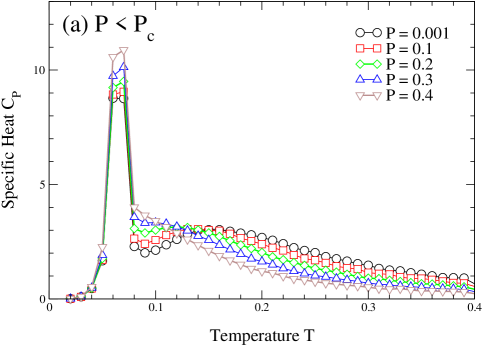
Figure 1: Monte Carlo Calculations: (a) Temperature dependence of the specific heat $C_{P}$, for the parameters in the text, along low pressure isobars with $P<P_{c}$. A broad maximum is visible along with a more pronounced one at lower $T$. The first maximum moves to lower $T$ as the pressure is raised and it merges with the low–$T$ maximum at $P\approx 0.4$. Upon approaching $P_{c}=0.70\pm 0.1$, the sharp maximum increases in value. (b) Same for $P\geq P_{c}$: the two maxima are separated only for $P>0.88$; the sharp maximum decreases as $P$ increases. In both panels errors are smaller than symbol size and lines are guides for the eyes.

From our MC simulations, we find that for low $P$ isobars, such as $P=0.001$, the model exhibits two $C_{P}$ maxima in the liquid state Mazza-PNAS11 . The maximum at higher $T$ is broad, while the maximum at lower $T$ is rather sharp (Fig. 1a).

Using MC simulations we find for several $P<P_{c}$ that the temperatures of the maxima of $C_{P}$ depend on $P$. As $P$ increases toward $P_{c}$, the sharp maximum remains relatively constant in $T$, while the higher-$T$ broad maximum moves to lower $T$. For $P\approx P_{c}$, the two maxima merge. The value of the sharp maximum slowly increases with increasing $P$, reaching the largest values at $P_{c}$ Note1 .

When $P>P_{c}$ the sharp maximum at lower-$T$ occurs at the temperature of the first-order LL phase transition (Fig. 1b). As $P$ increases far above $P_{c}$, the two maxima again separate in $T$. The sharp maximum decreases in value, and moves to lower $T$ with increasing $P$, following the LL phase transition. The broader $C_{P}$ maximum at higher $T$ becomes independent of $P$, as has been noted Marques-PRE07 ; Note2 . Hence as $P$ continues to increase, the maxima become further separated in $T$.

III.1.2 Mean Field Calculations

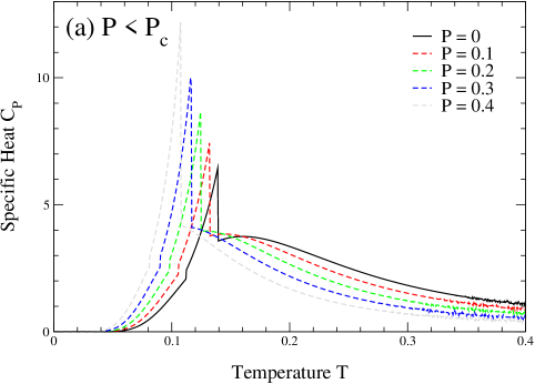
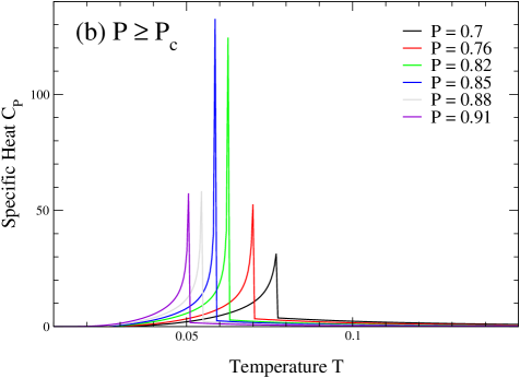
Figure 2: Mean Field Calculations: Same as in Fig. 1 but from mean field calculations (a) at $P<P_{c}^{\rm MF}$ and (b) at $P$ approaching or larger than $P_{c}^{\rm MF}$. The mean field critical pressure is $P_{c}^{\rm MF}=0.82\pm 0.04$. 

We also calculate $C_{P}$ within a MF approximation Franzese-JPCM02 ; PhysA02 ; Franzese-PRE03 ; KumarPRL2008 ; KumarJPCM2008 ; JPCM08 ; JPCM2010 ; PRER2012 . For $P<P_{c}$ we find qualitative behavior similar to that found in MC simulations (Fig. 2a). For $P=0$, $C_{P}$ exhibits two maxima. Both maxima move to lower $T$ as $P$ increases, though the broader maximum has a $P$-dependence that is more pronounced than that found in MC simulations. In MF, the two maxima are distinct only significantly below $P_{c}$; above $P\simeq 0.3$ both peaks merge into a single maximum. The $C_{P}$ maximum increases on approaching the MF critical pressure $P_{c}^{\rm MF}=0.82\pm 0.04$ (Fig. 2b). For $P>P_{c}^{\rm MF}$, $C_{P}$ exhibits only one maximum, marking the LL phase transition line. The higher-$T$ maximum at $P>P_{c}$ is not seen in the MF treatment of the model, as it is likely that bond variables satisfying the directional bond interaction and the cooperative bond interaction are not independent.

III.2 Origin of the two maxima in $C_{P}$

The origin of the two distinct maxima in $C_{P}$ may be understood by considering the enthalpy to be a sum of a contribution due to single H bond formation ($H^{\rm 1HB}$) and a term due to the cooperative interaction among bonds ($H^{\rm coop}$), i.e.,

$$H=H^{\rm 1HB}+H^{\rm coop},$$ (9)

with

$$H^{\rm 1HB} \equiv\langle-JN_{\rm HB}+PN_{\rm HB}v_{\rm HB}\rangle$$ (10)

$$H^{\rm coop} \equiv H-H^{\rm 1HB}.$$

Here, $H^{\rm 1HB}$ contains all terms proportional to $N_{\rm HB}$, and $H^{\rm coop}$ includes the enthalpy of the cooperative interaction, as well as the contribution coming from the van der Waals interaction, which is negligible in the range of $T$ of interest here.

From Eq. (9) we derive

$$C_{P}=C_{P}^{\rm 1HB}+C_{P}^{\rm coop},$$ (11)

where, by definition, for the MC model

$$C_{P}^{\rm 1HB}\equiv\left(\partial H^{\rm 1HB}/\partial T\right)_{P} =-(J-Pv_{\rm HB})(\partial\langle N_{\rm HB}\rangle/\partial T)_{P},$$ (12)

$$C_{P}^{\rm coop}\equiv\left(\partial H^{\rm coop}/\partial T\right)_{P} =P\left(\partial V_{0}/\partial T\right)_{P}-J_{\sigma}(\partial\langle N_{\rm coop}\rangle/\partial T)_{P}+(\partial\langle U_{W}(r)\rangle/\partial T)_{P},$$

and

$$N_{\rm coop}\equiv\sum_{i}n_{i}\sum_{(k,l)_{i}}\delta_{\sigma_{ik},\sigma_{il}}$$ (13)

is the total number of bond-index pairs that on each molecule minimize the cooperative interaction. In the low-$T$ region that we explore in this work, the isobaric variation of $V_{0}$ and $\langle U_{W}(r)\rangle$ with $T$ is negligible. Therefore, for the liquid at $T$ far below the liquid-gas transition, we can write

$$C_{P}^{\rm coop}\approx-J_{\sigma}(\partial\langle N_{\rm coop}\rangle/\partial T)_{P}.$$ (14)

A similar decomposition can be written also for the MF model, by replacing $\langle U_{W}(r)\rangle$ with $-\langle\epsilon\sum_{\langle i,j\rangle}n_{i}n_{j}\rangle$ in Eq. (12) and observing that its isobaric variation with $T$ is negligible in the low-$T$ region studied here.

III.2.1 Monte Carlo Calculations

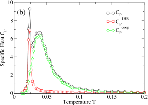
Figure 3: Monte Carlo Calculations: Decomposition of $C_{P}$ into the components $C_{P}^{\rm coop}$ and $C_{P}^{\rm 1HB}$, as in Eqs. (11-14), (a) for $P=0.1$, and (b) for $P=0.94$. Note that at low $P$ the high-$T$ broad $C_{P}$ maximum is due to $C_{P}^{\rm 1HB}$ and the sharp maximum at low $T$ is due to $C_{P}^{\rm coop}$. Vice versa at high $P$ the broader maximum at high $T$ is due to $C_{P}^{\rm coop}$ and the sharp maximum at low $T$ to $C_{P}^{\rm 1HB}$, inverting the order.

To understand which term in Eq. (11) is responsible for each maximum in $C_{P}$, we calculate separately the two contributions, as in Eqs. (12)–(14), and compare them with the direct calculation of $C_{P}$ from Eq. (7). We find that each term accounts for one and only one of the two maxima of $C_{P}$, as shown in Fig. 3. Furthermore, we observe that, for $P<P_{C}$ (Fig. 3a), $C_{P}^{\rm 1HB}$ is responsible for the maximum at higher $T$, while $C_{P}^{\rm coop}$ is responsible for the maximum at lower $T$. On the other hand, for $P>P_{C}$ (Fig. 3b), the two maxima invert their order, with the high-$T$ maximum due to $C_{P}^{\rm coop}$ and the low-$T$ maximum to $C_{P}^{\rm 1HB}$, and interchange their shape, with the one due to $C_{P}^{\rm 1HB}$ becoming broader and the one due to $C_{P}^{\rm coop}$ becoming sharper.

Equations (12–14) give us the key to understanding the nature of these two $C_{P}$ maxima. By definition $C_{P}$ is proportional to the isobaric variation of entropy with $T$. Therefore each maximum in $C_{P}$ corresponds to a maximum in the change of entropy, i.e., a maximum in a structural change. In particular, Eqs. (12)–(14) emphasize

• that the maximum in $C_{P}^{\rm 1HB}$ is associated with the largest isobaric variation of the number $N_{\rm HB}$ of H bonds with $T$, and

• that the maximum in $C_{P}^{\rm coop}$ is due to the largest variation with $T$ of the number $N_{\rm coop}$ of H bonds that minimize the cooperative interaction at constant $P$.

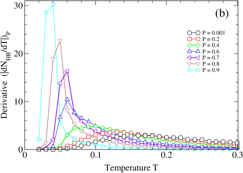
Figure 4: Monte Carlo Calculations: Temperature dependence of (a) the number of H bonds $N_{\rm HB}$, divided by the total number of possible H bonds $4N$, and (b) its $T$-derivative $(\partial\langle N_{\rm HB}\rangle/\partial T)_{P}$ as a function of $T$ for different isobars. The temperatures of the maxima of the derivative overlap with the temperatures of the maxima of $C_{P}^{\rm 1HB}$ in Fig. 1.

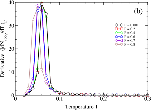
Figure 5: Monte Carlo Calculations: Temperature dependence of (a) the number $N_{\rm coop}$ of cooperative pairs of H bonds formed by the same molecule, divided by the total number of possible H bonds pairs on the same molecule $6N$, and (b) its $T$-derivative $(\partial\langle N_{\rm coop}\rangle/\partial T)_{P}$ as a function of $T$ for different isobars. The locus of the maxima of this derivative overlaps with the locus of the maxima of $C_{P}^{\rm coop}$ in Fig. 1.

These correspondences are verified by direct calculations of $(\partial\langle N_{\rm HB}\rangle/\partial T)_{P}$ and $(\partial\langle N_{\rm coop}\rangle/\partial T)_{P}$ (Figs. 4 and 5). We find that the loci of state points at which these derivatives are at a maximum overlap with the loci of maxima of $C_{P}^{\rm 1HB}$ and $C_{P}^{\rm coop}$, respectively. In Sec. IV we will discuss in more details the physical interpretation of these results.

III.2.2 Mean Field Calculations

Although the decomposition in Eq. (11) also applies to the MF model, in our MF approximation to solve the model, described in detail in Refs. Franzese-JPCM07 ; Stokely-book , we obtain

$$C_{P}\equiv\left(\frac{\partial H}{\partial T}\right)_{P}\approx 2(J-Pv_{\rm HB}+3J_{\sigma})\left(\frac{\partial p_{\sigma}}{\partial T}\right)_{P},$$ (15)

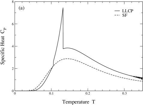
Figure 6: Mean Field Calculations: Comparison of $C_{P}$ calculations for the LLCP scenario case ($J_{\sigma}/\epsilon=0.05$) and the SF case ($J_{\sigma}=0$) (a) for $P=0.1$, and (b) for $P=0.9$. At low $P$, (a), the low-$T$ maximum is present only in the LLCP case, indicating that it is due to the cooperative term with $J_{\sigma}\neq 0$ in Eq. (6). At high $P$, (b), due to the mean field approximation we use, we find in both cases one single maximum in $C_{P}$. In the LLCP case, the maximum occurs at the LL phase transition temperature, while it occurs at lower $T$ in the SF case, for which no LL phase transition occurs.

where $p_{\sigma}$ is the probability that the facing bonding variables of two nearest neighbor molecules will be in the same state, but not necessarily in the state that minimizes the $J_{\sigma}$ cooperative interaction. The approximation consists in neglecting the liquid-gas contribution at low $T$. Because this expression for the specific heat cannot be easily separated into two terms, we calculate $C_{P}$ for the model either with or without cooperative interactions (Fig. 6). When including cooperative interactions ($J_{\sigma}>0$) the LLCP is present. Without them ($J_{\sigma}=0$) the SF scenario is obtained.

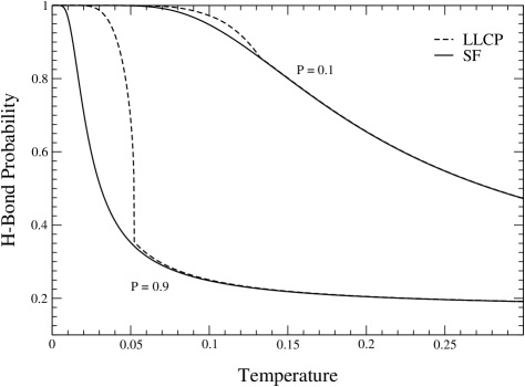
Figure 7: Mean Field Calculations: Probability of forming a H bond in the mean field approximation as a function of $T$, from which we calculate $C_{P}$, for $P=0.1.$ (upper curves) and $P=0.9.$ (lower curves), as indicated by the labels. The calculations for the LLCP scenario case ($J_{\sigma}/\epsilon=0.05$) are shown as dashed lines, and those for the SF case ($J_{\sigma}=0$) as continuous lines.

In the SF scenario the model is exactly solvable. We find that $C_{P}$ shows only one maximum, which is related to the isobaric $T$-derivative of $\langle N_{\rm HB}\rangle$ Sastry-PRE96 (Fig. 7). We find that at low $P$ (Fig. 6a) the SF maximum reproduces the LLCP high-$T$ broad maximum, has the same shape, and occurs at the same $T$. Thus the MF broad $C_{P}$ maximum at low $P$ is not related to the cooperative interaction, proportional to $J_{\sigma}$. Instead, because the sharper maximum at low $P$ is present only in the LLCP scenario, we conclude that it is due to the effect of the $J_{\sigma}$ cooperative term on the probability $p_{\rm HB}\equiv N_{\rm HB}/4N$ (Fig. 7) as a consequence of the maximum variation with $T$ of $\langle N_{\rm coop}\rangle$ at constant $P$. We thus find in MF indirect evidence that validates the proposed mechanism based on our MC calculations.

At $P>P_{c}$ (Fig. 6b), we observe in our MF solution only one maximum in $C_{P}$ with two large asymmetric tails, instead of the two maxima found in our MC calculations (Fig. 3b). We understand that this difference is caused by our MF approximation, Eq. (15). Nevertheless, we compare the calculations of $C_{P}$ without the $J_{\sigma}$ term to those with $J_{\sigma}$ term. We observe that without the $J_{\sigma}$ term (SF case), $C_{P}$ has a broad maximum at $T$ that is lower than the maximum found when the $J_{\sigma}$ term is present (LLCP case). This difference is evident from the behavior of $p_{\rm HB}$ in the two cases (Fig. 7). Thus at $P>P_{c}$ the cooperative $J_{\sigma}$ interaction contributes to $C_{P}$ at a $T$ that is higher than the contribution coming from the non-cooperative term, consistent with what we find in our MC calculations.

III.3 Isothermal Compressibility and Isobaric Thermal Expansivity

We also calculate the isothermal compressibility $K_{T}$ and the isobaric thermal expansivity $\alpha_{P}$, also known to exhibit anomalous behavior in bulk water. As with $C_{P}$, each of these depends upon $\langle N_{\rm HB}\rangle$

$$K_{T} =\frac{1}{V_{0}+\langle N_{\rm HB}\rangle v_{\rm HB}}\left[\left(\frac{\partial V_{0}}{\partial P}\right)_{T}+v_{\rm HB}\left(\frac{\partial\langle N_{\rm HB}\rangle}{\partial P}\right)_{T}\right]\approx\frac{v_{\rm HB}}{V_{0}+\langle N_{\rm HB}\rangle v_{\rm HB}}\left(\frac{\partial\langle N_{\rm HB}\rangle}{\partial P}\right)_{T},$$ (16)

$$\alpha_{P} =\frac{1}{V_{0}+\langle N_{\rm HB}\rangle v_{\rm HB}}\left[\left(\frac{\partial V_{0}}{\partial T}\right)_{P}+v_{\rm HB}\left(\frac{\partial\langle N_{\rm HB}\rangle}{\partial T}\right)_{P}\right]\approx\frac{v_{\rm HB}}{V_{0}+\langle N_{\rm HB}\rangle v_{\rm HB}}\left(\frac{\partial\langle N_{\rm HB}\rangle}{\partial T}\right)_{P},$$ (17)

where we use the observation that at low $T$ the variation of $V_{0}$ with $P$ and $T$ is negligible.

III.3.1 Monte Carlo Calculations

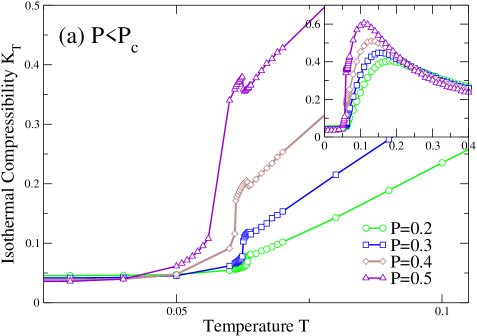
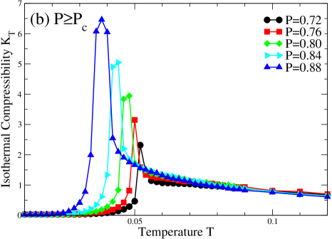
Figure 8: Monte Carlo Calculations: (a) Temperature dependence of the isothermal compressibility $K_{T}$ along low pressure isobars with $P<P_{c}$. Inset: the high-$T$ broad maximum. (b) Same for $P\geq P_{c}$.

At $P<P_{c}$, we find for $K_{T}$ a broad maximum that moves to lower $T$ upon increasing $P$ (inset Fig. 8a). This maximum occurs at higher $T$ with respect to the high-$T$ maximum that we find for $C_{P}$ (Fig. 1a). We also find a much smaller maximum of $K_{T}$ at a $T$ that coincides, within the error bars, with the low-$T$ maximum of $C_{P}$ (Fig. 1a).

At $P>P_{c}$, we find a single maximum of $K_{T}$ (Fig. 8b). This maximum follows the LL phase transition and the low-$T$ maximum of $C_{P}$ that we found for the same range of $P$ (Fig. 1b). The higher-$T$ maximum in $C_{P}$ for $P>P_{c}$ is not reflected in $K_{T}$, as the model includes no volume change for the cooperative rearrangement of the H bonds.

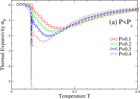
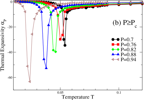
Figure 9: Monte Carlo Calculations: (a) Temperature dependence of the thermal expansivity $\alpha_{P}$ along low pressure isobars with $P<P_{c}$. (b) Same for $P\geq P_{c}$.

Our calculations of $|\alpha_{P}|$ at $P<P_{c}$ (Fig. 9a) show a behavior qualitatively similar to $C_{P}$ (Fig. 1a), with a broad maximum at higher $T$ and a sharp maximum at lower $T$. The $T$ of the sharp maximum remains constant for increasing $P$, while the higher-$T$ maximum decreases in $T$ with increasing $P$. At $P>P_{c}$, $|\alpha_{P}|$ shows a single maximum that follows the LL phase transition (Fig. 9b). As with $K_{T}$, there is no equivalent to the higher-$T$ maximum in $C_{P}$ at $P>P_{c}$, as the model includes no volume change for cooperative rearrangement of the H bonds.

III.3.2 Mean Field Calculations

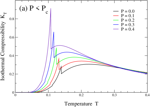
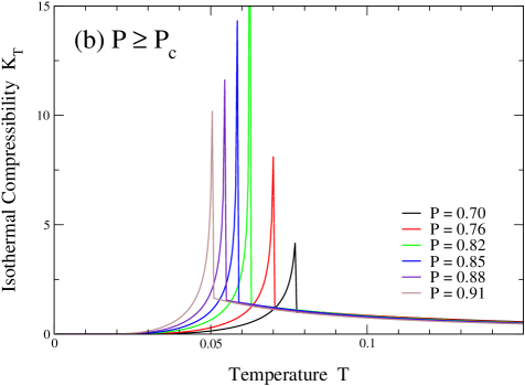
Figure 10: Mean Field Calculations: (a) Temperature dependence of the isothermal compressibility $K_{T}$ along low pressure isobars with $P<P_{c}$. (b) Same for $P\geq P_{c}$.

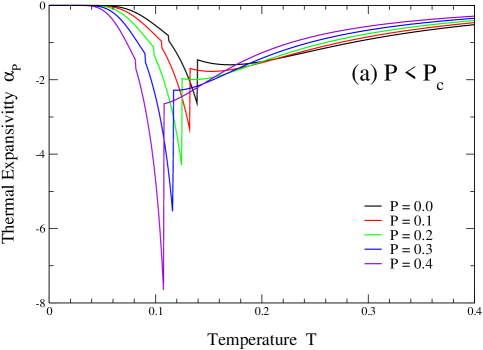
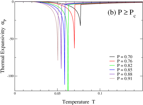
Figure 11: Mean Field Calculations: (a) Temperature dependence of the thermal expansivity $\alpha_{P}$ along low pressure isobars with $P<P_{c}$. (b) Same for $P\geq P_{c}$.

We can also calculate $K_{T}$ and $\alpha_{P}$ in the MF case. At $P<P_{c}$, $K_{T}$ (Fig. 10a) and $|\alpha_{P}|$ (Fig. 11a) exhibit two maxima, which also move closer in $T$ with increasing $P$. Because these quantities are proportional to derivatives of the MF calculation of the average number $\langle N_{\rm HB}\rangle$ of H bonds, as shown in Eqs. (16)–(17), we interpret the maxima as in the case of $C_{P}$, associating the high-$T$ maxima to the non-cooperative behavior and the low-$T$ maxima to the cooperative interaction.

At $P>P_{c}$, $K_{T}$ (Fig. 10b) and $|\alpha_{P}|$ (Fig. 11b) show each a single maximum that follows the LL phase transition. Also in this case the behavior is the same as what we find for the MF calculations of $C_{P}$.

IV Discussion

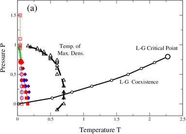
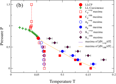
Figure 12: Monte Carlo Calculations: (a) Phase diagram showing the liquid–gas coexistence (continuous thick with circles) line, the temperature of maximum density (TMD, dashed thick with triangles) line, the LL coexistence line (pluses) ending in the LLCP (large full circle), and other lines that are better described in the second panel. (b) Magnification of the phase diagram at low $T$. At $P$ well below the LLCP, $C_{P}^{\rm coop}$ (empty squares), $\alpha_{P}^{\rm coop}$ (empty circles) and $K_{T}^{\rm coop}$ (empty diamonds), on one hand, and $C_{P}^{\rm 1HB}$ (filled squares), $\alpha_{P}^{\rm 1HB}$ (filled circles), and $K_{T}^{\rm coop}$ (filled diamonds), on the other hand, are maximal at different $T$. All the loci of maxima of $C_{P}$, $K_{T}$, and $|\alpha_{P}|$ converge toward the LLCP, together with the loci of maximal $({\rm d}N_{\rm coop}/{\rm d}T)_{P}$ (dark thin line) and $({\rm d}N_{\rm 1HB}/{\rm d}T)_{P}$ (light thin line), delimiting a region in the vicinity of the LLCP that approximates the Widom line. For $P>P_{c}$, all the loci coincide within the error with the LL coexistence line, but the locus of maximum $C_{P}^{\rm coop}$. If not shown, error bars are smaller that the symbol size.

The $P$–$T$ phase diagram of the model displays the liquid-gas critical point at the end of the first-order liquid-gas phase transition, the TMD line, the LLCP at the end of the first-order LL phase transition, the loci of maxima of the response functions that converge to each other, approximating the Widom line (Fig. 12a).

IV.1 Low-pressure region, Widom line and glassy temperature

Our results at low-$T$ show that the locus of the two maxima of $C_{P}$, which we denote as $C_{P}^{1HB}$ and $C_{P}^{\rm coop}$, correlate well with the locus of maxima of $({\rm d}N_{\rm HB}/{\rm d}T)_{P}$ and $({\rm d}N_{\rm coop}/{\rm d}T)_{P}$, respectively (Fig. 12b). We find the same close correlation with the structural changes of the H bond network for the loci of maxima of $K_{T}$ and $|\alpha_{P}|$ (Fig. 12b).

In a recent publication Mazza-PNAS11 , the proton relaxation time $\tau$ for a monolayer of water adsorbed onto the surface of the protein lysozyme was measured down to 150 K. This relaxation time is caused by charge defects moving along the H bond network, and thus probes the time-scale of H bond reorientation. It was found that the $T$-dependence of $\tau$ exhibits two crossovers in the region of the phase diagram in which two $C_{P}$ maxima are found in the present cell model.

The physical interpretation of these thermodynamic and dynamic results is straightforward. By decreasing $T$ at low $P$ the water molecules form an increasingly large number of H bonds. The largest structural change associated with this formation of H bonds is marked by the maximum in $(\partial\langle N_{\rm HB}\rangle/\partial T)_{P}$ (Fig. 4). Note that at any $P$ this maximum occurs where the probability $p_{B}\equiv N_{\rm HB}/(4N)$ of forming a H bond is approximately $p_{B}=0.8$ KumarJPCM2008 (Fig. 4). Although under these conditions the number of H bonds is macroscopic, they form independently, often with different relative orientations (bonding states). Thus at this stage the H bond regions that are thermodynamically correlated have a characteristic but finite size BIF2012 ; FBS2011 . Nevertheless, the formation of these finite clusters of correlated H bonds implies a change in their dynamics, with a crossover from a high-$T$ non-Arrhenius dynamics to a new regime at $T$ below the maximum of $(\partial\langle N_{\rm HB}\rangle/\partial T)_{P}$ and response functions, whose characteristics we discuss in the following.

As observed in Ref. KumarPRL2008 , at any $P$ the crossover occurs when the H bond relaxation time reaches a characteristic value. This value has been estimated to be $\tau=10^{-4}$ s in Ref. Mazza-PNAS11 , based on a comparison with dielectric spectroscopy experimental results for water adsorbed on lysozyme powder at a low hydration level (0.3 g H₂O/g dry protein). This time scale is seven orders of magnitude larger than the characteristic single molecule rotational relaxation time $\tau_{\rm rot}\simeq 28$ ps kumarPRE2006 at the same temperature of the crossover, $T\approx 252$ K. Thus the crossover is associated with a relaxation mode that involves more than one molecule, consistent with our interpretation based on finite clusters of correlated H bonds with a characteristic average size.

Although the first analysis suggested that the dynamics below the broad maximum of $C_{P}$ is Arrhenius KumarPRL2008 ; KumarJPCM2008 , further investigations extended to lower $T$ have shown that it is non-Arrhenius Mazza-PNAS11 . The dynamics becomes Arrhenius only at $T$ below the lower-$T$ maximum of $C_{P}$ Mazza-PNAS11 .

As discussed in Ref. Mazza-PNAS11 , we understand that the dynamic behavior is not Arrhenius between the two maxima of $C_{P}$ because at these temperatures the system has an activation energy that is $T$-dependent. This happens because interfaces with high free energy costs appear among the different clusters of correlated H bonds. By decreasing $T$ at constant $P$, the water many-body interaction, parametrized with $J_{\sigma}$ in the model, induces a cooperative rearrangement of the H bonds, gradually eliminating the interfaces among the clusters. This restructuring of the H bond clusters reaches its maximum when the $(\partial\langle N_{\rm coop}\rangle/\partial T)_{P}$ reaches its maximum (Fig. 5), resulting in the second maximum of $C_{P}$ (Fig. 1).

At this stage the cluster size of the correlated H bonds increases. As a consequence, a majority of the water molecules now have four H bonds that satisfy the cooperative interaction. Hence the dynamic behavior is dominated by processes with a characteristic activation energy. It has been shown by Mazza et al. that this activation energy is consistent with the average energy necessary to break a H bond in a cooperatively ordered environment Mazza-PNAS11 . Thus the dynamics has a second crossover below the low-$T$ maximum of $C_{P}$, this time to an Arrhenius behavior.

As consequence of the increase of the cluster size of the correlated H bonds, we identify, at low $P$ ($P<P_{c}$), the temperature of the low-$T$ crossover with the Widom line associated with the LL phase transition Limei-PNAS05 ; Franzese-JPCM07 . This suggests that previous works identifying a LL Widom line in supercooled water Limei-PNAS05 ; Franzese-JPCM07 ; JPCM08 ; Kumar2007 ; Mallamace2008 ; Abascal2010 may have only observed the higher–$T$ line of response maxima, the true Widom line residing at lower temperature.

The fact that this maximum occurs at an approximately constant value of $p_{\rm coop}\equiv N_{\rm coop}/(6N)\simeq 0.5$ at any $P$ (Fig. 5) implies that the cluster size of the correlated H bonds is independent of $P$. Analogous to what we have found for the first maximum of $C_{P}$, we expect this equal-cluster-size property at the crossover to correspond to an equal-characteristic-time at the crossover. Although at the present time we can only speculate this isocronic (equal time) property at the low-$T$ crossover, based on our comparison with the dielectric experimental results we predict the characteristic time to be of the order of 2 s Mazza-PNAS11 . This estimate is consistent with the idea that this crossover, and the Widom line, occurs at temperatures $T_{W}(P)$ that are above, but not far from, the glassy temperature $T_{g}(P)$ of the H bonds, defined as the temperature at which the H bond characteristic relaxation time exceeds 100 s. This conclusion is consistent with what has been recently found in long-time simulations for ST2 bulk water Kesselring2012 .

By increasing $P$, but with $P<P_{c}$, the increase in volume due to H bond formation contributes significantly to the enthalpy, making the H bonds unfavorable. Thus H bonds form at a $T$ that decreases with increasing $P$, and the maximum of $({\rm d}N_{\rm HB}/{\rm d}T)_{P}$ shifts to a lower $T$. On the other hand, the $T$ at which $({\rm d}N_{\rm coop}/{\rm d}T)_{P}$ is at a maximum remains approximately constant with $P$, as there is no volume cost associated with the cooperative rearrangement. Therefore the two maxima in $C_{P}$ move closer in $T$ when $P<P_{c}$ increases (Fig. 12).

The fact that the maximum of $({\rm d}N_{\rm coop}/{\rm d}T)_{P}$ does not depend much on $P$ implies that the cooperative maximum of $C_{P}$ and the Widom line of the LL phase transition also do not depend strongly on $P$. This prediction that the Widom line behavior is a weak function of $P$ has been confirmed recently by a fitting of the thermodynamic data based on the LLCP hypothesis Holten .

Although $K_{T}$ and $\alpha_{P}$ do not explicitly depends on $N_{\rm coop}$, they also show as $C_{P}$ a maximum at low $P$ and low $T$ that follows the maximum of $({\rm d}N_{\rm coop}/{\rm d}T)_{P}$. We understand this behavior as a consequence of the fact that $N_{\rm HB}$, from which $K_{T}$ and $\alpha_{P}$ depend, is affected by a large change of $N_{\rm coop}$, because by increasing the number $N_{\rm coop}$ of bonding indices of the same molecules in the same state, also the number $N_{\rm HB}$ of H bonds between different molecules increases at low $T$, spreading the local order at a distance that is of the order of the correlation length $\xi$.

Next, we discuss the difference of our findings with those presented for an isotropic potential describing an anomalous liquid, where two maxima of $C_{P}$ at different temperatures were observed in the supercritical region with respect to the LLCP Sergey09 . In this case the low-$T$ maximum is a consequence of the out-of-equilibrium dynamics of the system and is related to the glass transition temperature $T_{g}(P)$ of the liquid, as emphasized by the cooling-rate dependence of the low-$T$ maxima of the isotropic potential $C_{P}$ Sergey09 . In our case, as discussed above, all the maxima occur at $T>T_{g}(P)$. Furthermore, our calculations can be equilibrated at any $T$ thanks to the efficient Wolff algorithm, characterized by short MC correlation times mazzaCPC , consistent with our MF analysis that is, by definition, at equilibrium.

Finally, we observe that the molar heat capacities of the water confined within nano-pores of silica MCM-41 measured with adiabatic calorimetry for pores with 1.8 nm diameter shows two maxima Oguni-08 . The low-$T$ maximum in this case has been associated to the crystallization of part of the water in the pore Oguni-08 . In our case, we can exclude any crystallization effect by direct analysis of the dynamics of the system, consistent with previous simulations Zangi ; Kumar . A diffusion analysis has shown that our system is subdiffusive at the Widom line temperatures JPCB2011 ; PRER2012 , but not crystalline.

IV.2 The liquid-liquid critical point and the high-pressure region

When $P<P_{c}$, the response functions $C_{P}$, $K_{T}$, and $\alpha_{P}$ exhibit maxima that occur at temperatures that approach each other as $P$ increases (Fig. 12). For the same state points, the absolute values of their maxima increase and reach their maximum value when the loci of their maxima in the plane $P$-$T$ merge (Fig. 12b). This is the behavior we would expect at the critical point in a finite system, where by definition the value of the response functions cannot diverge. We therefore locate the LLCP ($P_{c}$, $T_{c}$) at the thermodynamic point where the maxima of the response functions and of $({\rm d}N_{\rm HB}/{\rm d}T)_{P}$, and $({\rm d}N_{\rm coop}/{\rm d}T)_{P}$ merge (Fig. 12b).

The LLCP occurs where both the structural change associated with $N_{\rm HB}$ and that associated with $N_{\rm coop}$ have their maxima. This is because at this state point the macroscopic increase in the number of H bonds is amplified by their simultaneous rearrangement into a cooperative configuration. This gives rise to a cooperative phenomenon that encompasses the entire system and causes a continuous change from a high-$T$, highly disordered, high-energy, high-density liquid (HDL) phase with a few H bonds, to a low-$T$, more ordered, low-energy, low-density (LDL) liquid phase with many cooperatively ordered H bonds.

When $P>P_{c}$, H bonds form at a $T$ that continues to decrease with increasing $P$, due to their enthalpic cost for the density decrease. This cost can be counterbalanced only by a large energy gain and entropy loss. This condition is realized only when the H bonds adopt the orientation that minimizes the many-body, cooperative interaction. Thus when a macroscopic number of H bonds is formed, the free energy of the system experiences a discontinuous change that results in a first-order phase transition. This transition is marked by sharp maxima in $C_{P}$, due to the $C_{P}^{1HB}$ component, $K_{T}$, and the absolute value of $\alpha_{P}$ (Fig. 12).

At $T$ higher than the LL phase transition, the few H bonds that have formed will themselves rearrange locally, resulting in a maximum of $({\rm d}N_{\rm coop}/{\rm d}T)_{P}$. This in turn implies a maximum in $C_{P}$ due to the $C_{P}^{\rm coop}$ component (Fig. 12).

V Summary and Conclusions

A microscopic cell model for a confined water monolayer that exhibits a LL phase transition and LLCP shows two maxima in $C_{P}$ at very low $T$. We decompose $C_{P}$ as a sum of two terms, $C_{P}^{\rm 1HB}$ and $C_{P}^{\rm coop}$, each of which is responsible for one of the maxima in $C_{P}$. We find that $C_{P}^{\rm 1HB}$ is caused by fluctuations in the formation of H bonds, while $C_{P}^{\rm coop}$ is caused by fluctuations arising from the cooperative interaction among H bonds. We find two maxima also in both $K_{T}$ and $\alpha_{P}$, occurring at the same temperatures as the two maxima of $C_{P}$.

A physical picture emerges from these results. The liquid at ambient conditions contains few molecules that form strong H bonds with neighboring molecules. At low $P$, upon cooling, the entropy cost of bond formation contributes less to the free energy, and bonds form independently. The rate of H bond formation, $(\partial\langle N_{\rm HB}\rangle/\partial T)_{P}$, reaches a maximum that is reflected in $C_{P}$ by the maximal contribution of $C_{P}^{\rm 1HB}$. With further cooling at low $P$, the H bonds reorganize into a more cooperative arrangement. This molecular reorganization is dominated by the small energy scale of the many-body interactions among the water molecules, occurring at the $T$ where $C_{P}$ has the maximal contribution of $C_{P}^{\rm coop}$.

Recent experimental results on a water monolayer hydrated lysozyme powder are consistent with the occurrence of the two $C_{P}$ maxima, as discussed in Ref. Mazza-PNAS11 . In the experiment, the H bond dynamics show two crossovers at separate temperatures. These are reproduced by the model, which shows that they are a consequence of the two $C_{P}$ maxima and the two associated structural changes. Thus the measurement of the two crossovers strongly supports the existence of two $C_{P}$ maxima in water at low $P$.

At higher $P$ the volume contribution to the enthalpy becomes more relevant. It affects the formation of the H bonds, causing the decrease of the temperature of maximum $C_{P}^{\rm 1HB}$. On the other hand, the volume change due to the cooperative rearrangement is assumed to be negligible in our approach, and $P$ has no effect on the locus of maximum $C_{P}^{\rm coop}$. The consistency of our predictions with a recent analysis of available experimental data Holten supports our assumption.

The $P$-dependence of the locus of maximum $C_{P}^{\rm 1HB}$, opposite to the $P$-independence of the locus of maximum $C_{P}^{\rm coop}$, allows us to predict that the two maxima of $C_{P}$ move closer in $T$ with increasing $P$ for $P\ll P_{c}$, to separate in $T$ with increasing $P$ for $P\gg P_{c}$, and to cross each other in the vicinity of $P_{c}$. For $K_{T}$ and $\alpha_{P}$, instead, the two maxima are present only for $P\ll P_{c}$, merging approaching $P_{c}$.

These predictions enable us to discriminate among the scenarios that have been proposed for the phase diagram of water, including the SF, LLCP, and CPF (or its equivalent SL) scenarios. In our study of the phase diagram of an adsorbed monolayer of water we find that each scenario predicts a unique behavior of $C_{P}$, $K_{T}$ and $\alpha_{P}$ at supercooled $T$. In particular, a measurement of the two crossovers in the dynamics Mazza-PNAS11 , interpreted as a consequence of the two maxima of $C_{P}$, rules out the SF scenario, because in the SF scenario there is only one maximum and, as a consequence, only one crossover.

Our predictions of different pressures also suggest an experimental test to discriminate between the LLCP and the CPF scenarios, i.e., a measurement of the $C_{P}$, or $K_{T}$ or $\alpha_{P}$ maxima at several pressures around ambient pressure under supercooled conditions. Indeed, at low $P$ the two maxima in the response functions should approach each other if the LLCP scenario holds. If, instead, the CPF scenario is verified or if the LLCP occurs at a pressure below those investigated, the two maxima of $C_{P}$ should separate further, while $K_{T}$ and $\alpha_{P}$ should have only one maximum. Thus by measuring how these maxima move in $T$ at several $P$ we could determine whether (i) the two maxima of $C_{P}$, or $K_{T}$ or $\alpha_{P}$ merge at positive $P$, giving a lower-bound estimate of the LLCP, (ii) the two maxima of $C_{P}$ merge at negative $P$ above the limit of stability of the liquid with respect to the gas, giving an upper-bound estimate of the LLCP, or (iii) the two maxima of $C_{P}$ do not merge before the liquid-to-gas limit of stability, ruling out the LLCP and supporting the CPF scenario.

VI Acknowledgments

We thank F. Mallamace, S. Sastry and E. Strekalova for helpful discussions. We acknowledge the support of NSF grants CMMI-1125290, CHE-0404673, CHE-0911389 and CHE-0908218, and GF the Spanish MICINN grant FIS2007-61433 (co-financed FEDER) and the EU FP7 grant NMP4-SL-2011-266737.

References

- (1) P. G. Debenedetti, J. Phys.: Condens. Matter 15, R1669 (2003); P. G. Debenedetti and H. E. Stanley, Physics Today 56[6], 40 (2003).
- (2) C. A. Angell, Science 319, 582 (2008); F. Mallamace et al., Rivista del Nuovo Cimento 34, 253 (2011).
- (3) P. Ball, Nature 478, 467 (2011).
- (4) V. Bianco, et al., J. Bio. Phys. 38, 27 (2012).
- (5) F. Franks, Water: A Comprehensive Treatise (Plenum Press, New York, 1972).
- (6) R. J. Speedy and C. A. Angell, J. Chem. Phys. 65, 851 (1976).
- (7) E. Tombari, C. Ferrari, and G. Salvetti, Chem. Phys. Lett. 300, 749 (1999).
- (8) R. J. Speedy, J. Phys. Chem. 86 3002 (1982).
- (9) S. Sastry et al., Phys. Rev. E 53, 6144 (1996).
- (10) H. E. Stanley and J. Teixeira, J. Chem. Phys. 73, 3404 (1980); H. E. Stanley, J. Phys. A 12, L329 (1979).
- (11) L. P. N. Rebelo, P. G. Debenedetti, and S. Sastry, J. Chem. Phys. 109, 626 (1998).
- (12) P. H. Poole et al., Nature (London) 360, 324 (1992).
- (13) L. Xu et al., Proc. Natl. Acad. Sci. USA 102, 16558 (2005).
- (14) G. Franzese and H. E. Stanley, J. Phys.: Condens. Matter 19, 205126 (2007).
- (15) E. B. Moore and V. Molinero, J. Chem. Phys. 130, 244505 (2009).
- (16) P. H. Poole, I. Saika-Voivod, and F. Sciortino, J. Phys.: Condens. Matter 17, L431 (2005).
- (17) D. A. Fuentevilla and M. A. Anisimov, Phys. Rev. Lett. 97, 195702 (2006); C. E. Bertrand, and M. A. Anisimov, J. Phys. Chem. B 115, 14099 (2011).
- (18) Y. Liu, A. Z. Panagiotopoulos, and P. G. Debenedetti, J. Chem. Phys. 131, 104508 (2009); see also D. T. Limmer, and D. Chandler, J. Chem. Phys. 135, 134503 (2011) for a criticism to this work, and F. Sciortino, I. Saika-Voivod, and P. H. Poole, Phys. Chem. Chem. Phys. 13, 19759 (2011) for an answer to the criticism.
- (19) J. L. F. Abascal and C. Vega, J. Chem. Phys. 133, 234502 (2010); ibid. 134, 186101 (2011).
- (20) P. H. Poole, S. R. Becker, F. Sciortino, and F. W. Starr, J . Phys. Chem. B 115, 14176 (2011).
- (21) T. A. Kesselring et al., Scientific Reports 2, 474, doi:10.1038/srep00474 (2012).
- (22) V. Holten, C. E. Bertrand, M. A. Anisimov, and J. V. Sengers, J. Chem. Phys. 136, 094507 (2012); V. Holten and M. A. Anisimov, “Entropy-driven liquid-liquid separation in supercooled water”, arXiv:1207.2101 (2012).
- (23) H. Tanaka, Nature (London) 380, 328 (1996).
- (24) P. H. Poole et al., Phys. Rev. Lett. 73, 1632 (1994).
- (25) K. Stokely et al., Proc. Natl. Acad. Sci. USA 107, 1301 (2010).
- (26) T. Takamuku, M. Yamagami, H. Wakita, Y. Masuda, and T. Yamaguchi, J. Phys. Chem. B 101, 5730 (1997); H. K. Christenson, J. Phys: Condens. Matter 13, R95 (2001).
- (27) A. K., Soper, Mol. Phys. 106, 2053 (2008).
- (28) E. G. Strekalova et al., Phys. Rev. Lett. 106, 145701 (2011).
- (29) E. G. Strekalova et al., J. Phys.: Condens. Matter 24 064111 (2012).
- (30) E. G. Strekalova et al., Phys. Rev. Lett. xx, xxxxxx (2012).
- (31) L. Xu, and V. Molinero, J. Phys. Chem. B 115, 14210 (2011).
- (32) G. T. Baechle, G. P. Eberli, R. J. Weger, and J. L. Massaferro, Geophys, 74, E135 (2009); P. Baud, W. Zhu, and T.-F. Wong, J. Geophys. Res. 105 16371 (2000).
- (33) U. Lohmann and J. Feichter, Atmos. Chem. Phys. 5, 715 (2005).
- (34) L. R. Merte et al., Science 336, 889 (2012).
- (35) J. Israelachvili and H. Wennerström, Nature (London) 379, 219 (1996); G. Careri, Prog. Biophys. Mol. Biol. 70, 223 (1998).
- (36) S.-H. Chen et al., Proc. Natl. Acad. Sci. USA 103, 9012 (2006).
- (37) H. Frauenfelder et al., Proc. Nat. Acad. Sci. USA 106, 5129 (2009).
- (38) M. G. Mazza et al., Proc. Natl. Acad. Sci. USA 108, 19873 (2011).
- (39) K. Koga, H. Tanaka, and X. C. Zeng, Nature (London) 408, 564 (2000).
- (40) R. Zangi and A. E. Mark, Phys. Rev. Lett. 91, 025502 (2003).
- (41) P. Kumar et al., Phys. Rev. E 72, 051503 (2005).
- (42) G. Franzese and H. E. Stanley, J.Phys.: Condens. Matter 14, 2201 (2002).
- (43) G. Franzese and H. E. Stanley, Physica A 314, 508 (2002).
- (44) G. Franzese, M. I. Marqués, and H. E. Stanley, Phys. Rev. E 67, 011103 (2003).
- (45) P. Kumar et al., Phys. Rev. Lett. 100, 105701 (2008).
- (46) P. Kumar et al., J. Phys.: Condens. Matter 20, 244114 (2008).
- (47) G. Franzese et al., J. Phys.: Condens. Matter 20, 494210 (2008).
- (48) G. Franzese and F. de los Santos, J. Phys.: Condens. Matter 21, 504107 (2009).
- (49) G. Franzese et al., J. Phys.: Condens. Matter 22, 284103 (2010).
- (50) G. Franzese, V. Bianco, and S. Iskrov, Food Biophysics 6, 186 (2011).
- (51) F. de los Santos and G. Franzese, J. Phys. Chem. B 115, 14311 (2011).
- (52) F. de los Santos and G. Franzese, Phys. Rev. E 85, 010602(R) (2012).
- (53) H. S. Frank, W. Y. Wen, Discuss. Faraday Soc. 24, 133 (1957).
- (54) R. Ludwig, Angew. Chem. Int. Ed. 40, 1808 (2001).
- (55) M. A. Ricci, F. Bruni, and A. Giuliani, Faraday Disc. 141, 347 (2009).
- (56) A. K. Soper and M. A. Ricci, Phys. Rev. Lett. 84, 2881 (2000).
- (57) A. M. Saitta and F. Datchi, Phys. Rev. E 67 020201(R) (2003).
- (58) U. Wolff, Phys. Rev. Lett. 62, 361 (1989).
- (59) M. G. Mazza et al., Comput. Phys. Commun. 180, 497 (2009).
- (60) V. Cataudella et al., Phys. Rev. Lett. 72, 1541 (1994).
- (61) V. Cataudella et al., Phys. Rev. E 54, 175 (1996).
- (62) G. Franzese, Phys. Rev. E 61, 6383 (2000).
- (63) O. Vilanova and G. Franzese, “Structural and dynamical properties of nanoconfined supercooled water,” arXiv:1102.2864 (2011).
- (64) Our resolution in does not allow us to observe the expected divergence of upon approaching the critical point.
- (65) M. I. Marqués, Phys. Rev. E 76, 021503 (2007).
- (66) The difference of our results with those in Marques-PRE07 , i.e., the presence of two maxima also at and is due to the different choice of parameters for the model: here as in PhysA02 ; Stokely-PNAS10 ; Franzese-JPCM02 ; Franzese-PRE03 , while in Marques-PRE07 is , which gives rise to a different phase diagram.
- (67) K. Stokely et al., “Metastable Water under Pressure” in Metastable Systems under Pressure (NATO Science for Peace and Security Series A: Chemistry and Biology) (Berlin: Springer, 2010), pp. 197–216.
- (68) P. Kumar et al., Phys. Rev. E 73, 041505 (2006).
- (69) P. Kumar et al., Proc. Natl. Acad. Sci. USA 104, 9575 (2007).
- (70) F. Mallamace et al. Proc. Natl. Acad. Sci. USA 105, 12725 (2008).
- (71) S. V. Buldyrev et al., J. Phys.: Condens. Matter 21, 504106 (2009).
- (72) M. Oguni, Y. Kanke, and S. Namba, AIP Conference Proceedings 982, 34 (2008).