Connections of activated hopping processes with the breakdown of the Stokes-Einstein relation and with aspects of dynamical heterogeneities

Abstract

We develop a new extended version of the mode-coupling theory (MCT) for glass transition, which incorporates activated hopping processes via the dynamical theory originally formulated to describe diffusion-jump processes in crystals. The dynamical-theory approach adapted here to glass-forming liquids treats hopping as arising from vibrational fluctuations in quasi-arrested state where particles are trapped inside their cages, and the hopping rate is formulated in terms of the Debye-Waller factors characterizing the structure of the quasi-arrested state. The resulting expression for the hopping rate takes an activated form, and the barrier height for the hopping is “self-generated” in the sense that it is present only in those states where the dynamics exhibits a well defined plateau. It is discussed how such a hopping rate can be incorporated into MCT so that the sharp nonergodic transition predicted by the idealized version of the theory is replaced by a rapid but smooth crossover. We then show that the developed theory accounts for the breakdown of the Stokes-Einstein relation observed in a variety of fragile glass formers. It is also demonstrated that characteristic features of dynamical heterogeneities revealed by recent computer simulations are reproduced by the theory. More specifically, a substantial increase of the non-Gaussian parameter, double-peak structure in the probability distribution of particle displacements, and the presence of a growing dynamic length scale are predicted by the extended MCT developed here, which the idealized version of the theory failed to reproduce. These results of the theory are demonstrated for a model of the Lennard-Jones system, and are compared with related computer-simulation results and experimental data.

I Introduction

The decoupling of the self-diffusion constant from the viscosity or the structural relaxation time – also referred to as the breakdown of the Stokes-Einstein (SE) relation – that occurs for temperatures $T\lesssim 1.2\,T_{\rm g}$ near the glass transition temperature $T_{\rm g}$ is among the most prominent features of fragile glass formers Chang and Sillescu (1997); Swallen et al. (2003); Mapes et al. (2006). The decoupling has been considered as one of the signatures of spatially heterogeneous dynamics or “dynamical heterogeneities” Ediger (2000); Xia and Wolynes (2001); Berthier (2004); Jung et al. (2004). On the other hand, it is also well recognized that the onset temperature $\approx 1.2\,T_{\rm g}$ of the decoupling is close to a crossover temperature at which transport properties change their characters Rössler (1990) and below which the dynamics is thought to be dominated by activated hopping processes over barriers Goldstein (1969). Then, a natural question arises as to possible connections among the decoupling, dynamical heterogeneities, and the hopping processes. In this paper, such connections are explored by extending the idealized mode-coupling theory (MCT) for glass transition Götze (1991).

The idealized MCT has been known as the most successful microscopic theory for glass transition. Indeed, extensive tests of the theoretical predictions carried out so far against experimental data and computer-simulation results suggest that the theory deals properly with some essential features of glass-forming liquids Götze and Sjögren (1992); Götze (1999). On the other hand, a well-recognized limitation of the idealized MCT is the predicted divergence of the $\alpha$-relaxation time at a critical temperature $T_{\rm c}$ – also referred to as the nonergodic transition – which is not observed in experiments and computer simulations. An extended version of MCT developed in Ref. Götze and Sjögren (1987) aims at incorporating activated hopping processes which smear out the sharp nonergodic transition and restore ergodicity for $T\leq T_{\rm c}$, but its applicability has been restricted to schematic models. This is because of the presence of the subtraction term in the expression for the hopping kernel, which violates the positiveness – a fundamental property – of any correlation spectrum.

There have been relatively few other attempts to go beyond the idealized MCT Kawasaki (1994); Schweizer and Saltzman (2003); Bhattacharyya et al. (2005), and incorporating the hopping processes into the theory for glass transition has been a major unsolved problem. We present here a new formulation which is motivated by ideas from the dynamical theory originally developed to describe diffusion-jump processes in crystals Fly . The dynamical-theory approach adapted in this work to glass-forming liquids treats hopping as arising from vibrational fluctuations in quasi-arrested state where particles are trapped inside their cages, and the hopping rate is formulated in terms of the Debye-Waller factors characterizing the structure of the quasi-arrested state. The resulting expression for the hopping rate takes an activated form, and the barrier height for the hopping is “self-generated” in the sense that it is present only in those states where the dynamics exhibits a well defined plateau. It will be discussed how such a hopping rate can be incorporated to develop a new extended version of MCT.

We will then investigate whether the developed theory accounts for the mentioned decoupling for $T\lesssim T_{\rm c}$. Such an investigation makes sense since $T_{\rm c}$ is also found to be close to $1.2\,T_{\rm g}$ Rössler (1990), i.e., the onset temperature of the decoupling Chang and Sillescu (1997); Zöllmer et al. (2003). It will also be examined whether our theory reproduces characteristic features of dynamical heterogeneities revealed by recent computer simulations. More specifically, we shall study whether the theory predicts a substantial increase of the non-Gaussian parameter Kob et al. (1997), double-peak structure in the probability distribution of particle displacements Flenner and Szamel (2005a, b), and the presence of a growing dynamic length scale Berthier (2004), which the idealized MCT failed to reproduce.

The paper is organized as follows. In Sec. II, we formulate our new extended MCT. Numerical results of the theory are presented in Sec. III for a model of the Lennard-Jones system, and connections of the hopping processes with the breakdown of the SE relation and with aspects of dynamical heterogeneities are discussed. The paper is summarized in Sec. IV. Appendix A outlines a novel derivation of the hopping kernel formulated in Ref. Götze and Sjögren (1987), and Appendix B is devoted to the derivation of the extended-MCT equations for the mean-squared displacement and the non-Gaussian parameter.

II Theory

We start from surveying basic features of the idealized MCT Götze (1991) (see also Appendix A). A system of $N$ atoms of mass $M$ distributed with density $\rho$ shall be considered. Structural changes as a function of time $t$ are characterized by coherent density correlators $\phi_{q}(t)=\langle\rho_{\vec{q}}^{*}\,e^{i{\cal L}t}\rho_{\vec{q}}\rangle/NS_{q}$. Here $\rho_{\vec{q}}=\sum_{i}\exp(i{\vec{q}}\cdot{\vec{r}}_{i})$ with ${\vec{r}}_{i}$ referring to $i$th particle’s position denotes density fluctuations for wave vector ${\vec{q}}$; ${\cal L}$ the Liouville operator; $\langle\cdot\rangle$ the canonical averaging for temperature $T$; $S_{q}=\langle\rho_{\vec{q}}^{*}\,\rho_{\vec{q}}\rangle/N$ the static structure factor; and $q=|\,{\vec{q}}\,|$. Within the Zwanzig-Mori formalism Hansen and McDonald (1986) one obtains the following exact equation of motion:

$$\partial_{t}^{2}\phi_{q}(t)+\Omega_{q}^{2}\phi_{q}(t)+\Omega_{q}^{2}\int_{0}^{t}dt^{\prime}\,m_{q}(t-t^{\prime})\,\partial_{t^{\prime}}\phi_{q}(t^{\prime})=0.$$ (1a)

Here $$\Omega_{q}^{2}=q^{2}k_{\rm B}T/MS_{q} k_{\rm B} m_{q}(t) f(z)=i\int_{0}^{\infty}dt\,e^{izt}f(t) {\rm Im}\,z>0$$ with Boltzmann’s constant , and the memory kernel describes correlations of fluctuating forces. Introducing the Laplace transform with the convention (), Eq. (1a) is equivalent to the representation

$$\phi_{q}(z)=-1\,/\,\{z-\Omega_{q}^{2}\,/\,[z+\Omega_{q}^{2}\,m_{q}(z)]\}.$$ (1b)

Under the mode-coupling approximation, the fluctuating forces are approximated by their projections onto the subspace spanned by pair-density modes $\rho_{\vec{k}}\rho_{\vec{p}}$. The factorization approximation for dynamics of the pair-density modes yields the following idealized-MCT expression for the memory kernel to be denoted as $m_{q}^{\rm id}(t)$:

$$m_{q}^{\rm id}(t)=\int d{\vec{k}}\,V({\vec{q}};{\vec{k}},{\vec{p}}\,)\,\phi_{k}(t)\,\phi_{p}(t).$$ (2a)

Here $${\vec{p}}={\vec{q}}-{\vec{k}}$$, and the vertex function is given by

$$V({\vec{q}};{\vec{k}},{\vec{p}}\,)=\frac{\rho}{2(2\pi)^{3}q^{4}}S_{q}S_{k}S_{p}[({\vec{q}}\cdot{\vec{k}})c_{k}+({\vec{q}}\cdot{\vec{p}})c_{p}]^{2},$$ (2b)

in terms of $S_{q}$ and the direct correlation function $c_{q}=(1-1/S_{q})/\rho$. The idealized-MCT equations (1) and (2) exhibit a bifurcation for $\phi_{q}(t\to\infty)=f_{q}$ – also referred to as the nonergodic transition – at a critical temperature $T_{\rm c}$ Götze (1991). For $T>T_{\rm c}$, the correlator relaxes towards $f_{q}=0$ as expected for ergodic liquid states. On the other hand, density fluctuations for $T\leq T_{\rm c}$ arrest in a disordered solid, quantified by a Debye-Waller factor $f_{q}>0$.

It is the factorization approximation [cf. Eq. (24)] that leads to the nonergodic transition at $T_{\rm c}$. Therefore, one has to consider corrections, $m_{q}(z)=m_{q}^{\rm id}(z)+\Delta m_{q}(z)$, to go beyond the idealized MCT, which shall be quantified via the hopping kernel defined by

$$\delta_{q}(z)=-1/m_{q}(z)+1/m_{q}^{\rm id}(z).$$ (3a)

The correction term reads $$\Delta m_{q}(z)=m_{q}^{\rm id}(z)\delta_{q}(z)m_{q}(z) m_{q}(z)$$, and the memory kernel can be expressed as

$$m_{q}(z)=m_{q}^{\rm id}(z)\,/\,[\,1-\delta_{q}(z)\,m_{q}^{\rm id}(z)\,].$$ (3b)

As demonstrated in Appendix A, one can derive based on Eq. (3a) an expression for $\delta_{q}(z)$ which is essentially the same as that of the extended MCT of Götze and Sjögren Götze and Sjögren (1987, 1995) by applying the Zwanzig-Mori formalism to $m_{q}(t)$ and then introducing the corresponding mode-coupling approximation for the “memory kernel” to $m_{q}(t)$. Such a hopping kernel, however, retains the same problem mentioned in Sec. I. Instead, our attempt for the extension of the idealized MCT is motivated by the following observation: substituting Eq. (3b) into Eq. (1b) yields for small $z$ Götze and Sjögren (1992)

$$\phi_{q}(z)=-1\,/\,\{z+\delta_{q}(z)-\Omega_{q}^{2}\,/\,[z+\Omega_{q}^{2}\,m_{q}^{\rm id}(z)]\}.$$ (4)

Dropping $\delta_{q}(z)$, this equation reduces to the one of the idealized MCT: approaching $T_{\rm c}$ from above, $m_{q}^{\rm id}(z)$ for small $z$ becomes larger, and so does $\phi_{q}(z)$, leading to the nonergodic transition at $T=T_{\rm c}$. In the presence of $\delta_{q}(z)$, on the other hand, the transition is cutoff since the third term in the denominator of Eq. (4) becomes unimportant when $m_{q}^{\rm id}(z)$ becomes large. The long-time dynamics of $\phi_{q}(t)$ in this case is thus determined by $\delta_{q}(z)$ for small $z$. This observation raises a possibility of constructing a new approximate theory for $\delta_{q}(z)$ described below.

We first derive a rate formula for a hopping process in which an atom at ${\vec{r}}_{i}$ jumps to a nearby site ${\vec{r}}_{i}^{\,\prime}$ separated by an interparticle distance. The presence of such a process at low temperatures has been revealed by computer simulations Roux et al. (1989); Wahnström (1991); Schøder et al. (2000). This will be done via the dynamical theory originally developed to describe diffusion-jump processes in crystals Fly . The approach adapted here to glass-forming liquids treats hopping as arising from vibrational fluctuations (phonons) in quasi-arrested state where particles are trapped inside their cages. Let us suppose that the quasi-arrested state characterized by the Debye-Waller factors $f_{q}$ can be described as a frozen, irregular lattice Barrat et al. (1989). Each particle then has a well defined equilibrium position ${\vec{R}}_{i}$ within the lifetime of the quasi-arrested state, and we introduce the displacement from the equilibrium position via ${\vec{r}}_{i}={\vec{R}}_{i}+{\vec{u}}({\vec{R}}_{i})$. The essential feature of the hopping process is that a jumping atom passes over a barrier formed by neighbors which block a direct passage to the new site. The criterion that determines whether or not a given fluctuation is sufficient to cause a jump is therefore concerned with the relative displacements of the atom and the saddlepoint. We thus employ as a “reaction coordinate” Fly , $x(t)=[{\vec{u}}({\vec{R}}_{i}+{\vec{s}},t)-{\vec{u}}({\vec{R}}_{i},t)]\cdot\hat{\vec{s}}$, and assume that a hopping occurs when $x(t)$ exceeds a critical value $x^{*}$, which measures the size of fluctuation needed to cause a jump. Here ${\vec{s}}$ denotes the saddlepoint position with respect to ${\vec{R}}_{i}$, and the scalar product selects only those fluctuations directed towards $\hat{\vec{s}}={\vec{s}}/s$. Each phonon displaces a hopping atom towards the saddlepoint. The phonon phases are random, but the displacements may occasionally coincide in such a way that a hopping process occurs. The hopping rate $w_{\rm hop}$ can then be calculated from such a probability per unit time, and one obtains along the line described in Ref. Fly with the isotropic Debye approximation, $w_{\rm hop}=(1/2\pi)(3/5)^{1/2}\omega_{\rm D}\exp[-3mv^{2}\Delta^{2}/2k_{\rm B}T]$, in terms of the sound velocity $v$. Here $\omega_{\rm D}=k_{\rm D}v$ with the Debye wave number $k_{\rm D}=(6\pi^{2}\rho)^{1/3}$, and $\Delta\equiv x^{*}/s$. Notice that the sound velocity here refers to the one in the quasi-arrested state, which is renormalized by the Debye-Waller factors Götze and Mayr (2000); Chong (2006). To emphasize this, the sound velocity shall be expressed as $v=\sqrt{M_{\rm L}/(\rho m)}$ in terms of the (longitudinal) elastic modulus

$$M_{\rm L}=M_{\rm L}^{0}+\delta M_{\rm L},$$ (5a)

consisting of the equilibrium value $$M_{\rm L}^{0}=\rho(k_{\rm B}T)/S_{0} S_{0}\equiv S_{q\to 0}$$, where , and an additional contribution for the quasi-arrested state, for which MCT yields Götze and Sperl (2003)

$$\delta M_{\rm L}=\rho(k_{\rm B}T)\int dk\,V_{\rm L}(k)f_{k}^{2},$$ (5b)

with

$$V_{\rm L}(k)=\frac{\rho k^{2}S_{k}^{2}}{4\pi^{2}}\left\{c_{k}^{2}+\frac{2}{3}[kc_{k}^{\prime}]c_{k}+\frac{1}{5}[kc_{k}^{\prime}]^{2}\right\}.$$ (5c)

The hopping rate is then given by

$$w_{\rm hop}=\frac{1}{2\pi}\left(\frac{3}{5}\right)^{\frac{1}{2}}\omega_{\rm D}\exp\left[-\frac{3M_{\rm L}}{2\rho k_{\rm B}T}\,\Delta^{2}\right].$$ (6)

The pre-exponential factor represents a mean attack frequency while the exponential term of the activated form gives the probability that the system is found at the critical displacement $x^{*}$. In addition, the barrier height for the hopping is “self-generated” in the sense that it is determined by the plateau heights $f_{q}$ of the coherent density correlators, and is present only in those states where the dynamics exhibits a well defined plateau.

We next relate the hopping rate $w_{\rm hop}$ to the hopping kernel $\delta_{q}(z)$. Our discussion becomes simpler if the tagged-particle density correlator $\phi_{q}^{s}(t)$ – the self part of $\phi_{q}(t)$ – is considered, so this case shall be considered first. Hereafter, quantities referring to the tagged particle shall be marked with the superscript or subscript “$s$”. The Zwanzig-Mori equation for $\phi_{q}^{s}(t)$ has the same form as Eq. (1a) with $\phi_{q}$, $m_{q}$, and $\Omega_{q}^{2}$ replaced by $\phi_{q}^{s}$, $m_{q}^{s}$, and $(\Omega_{q}^{s})^{2}=q^{2}k_{\rm B}T/M$, respectively; the idealized-MCT kernel corresponding to Eq. (2a) is given by $m_{q}^{s\,{\rm id}}(t)=\int d{\vec{k}}\,V^{s}({\vec{q}};{\vec{k}},{\vec{p}})\phi_{k}(t)\phi_{p}^{s}(t)$ with $V^{s}=\rho S_{k}[({\vec{q}}\cdot{\vec{k}})c_{k}]^{2}/[(2\pi)^{3}q^{4}]$ Fuchs et al. (1998); and Eq. (3b) holds with $m_{q}$, $m_{q}^{\rm id}$, and $\delta_{q}$ replaced by $m_{q}^{s}$, $m_{q}^{s\,{\rm is}}$, and $\delta_{q}^{s}$, respectively. The arrested part $f_{q}^{s}$ of the correlator $\phi_{q}^{s}(t)$ is referred to as the Lamb-Mössbauer factor.

In the absence of the hopping kernel, the idealized kernel $m_{q}^{s\,{\rm id}}(t)$ for $T\leq T_{\rm c}$ arrests at a plateau for long times whose height is given by $C_{q}^{s}=f_{q}^{s}/(1-f_{q}^{s})$ Götze (1991), i.e., there holds $m_{q}^{s\,{\rm id}}(z)=-C_{q}^{s}/z$ for small $z$. Substituting this into Eq. (4) for $\phi_{q}^{\rm s}(z)$ yields for small $z$

$$\phi_{q}^{s}(z)=-f_{q}^{s}/[z+f_{q}^{s}\delta_{q}^{s}(z)],$$ (7)

which determines the $\alpha$ relaxation of $\phi_{q}^{s}(t)$ – the decay from the plateau $f_{q}^{s}$ to zero – in the presence of $\delta_{q}^{s}(z)$.

On the other hand, when the $\alpha$ relaxation is dominated by hopping processes characterized by a rate $w_{\rm hop}({\vec{r}}\to{\vec{r}}^{\,\prime})$, the van Hove self correlation function $G_{s}({\vec{r}},t)$, related to $\phi_{q}^{s}(t)$ via the inverse Fourier transform

$$G_{s}({\vec{r}},t)=\frac{1}{(2\pi)^{3}}\int d{\vec{q}}\,e^{-i{\vec{q}}\cdot{\vec{r}}}\,\phi_{q}^{s}(t),$$ (8)

and proportional to the probability of finding the tagged particle at ${\vec{r}}$ and $t$ Hansen and McDonald (1986), obeys a simple rate equation

$$\partial_{t}G_{s}({\vec{r}},t) = \sum_{\vec{l}}[\,w_{\rm hop}({\vec{r}}+{\vec{l}}\to{\vec{r}})G_{s}({\vec{r}}+{\vec{l}},t)$$ (9)

$$\qquad\quad-\,w_{\rm hop}({\vec{r}}\to{\vec{r}}+{\vec{l}})G_{s}({\vec{r}},t)\,].$$

We assume that only hoppings with $|\,{\vec{l}}\,|\approx a$ are relevant, in which $a\equiv\int_{0}^{r_{\rm min}}dr\,r\left[N(r)/N_{\rm c}\right]$ denotes the weighted average of interparticle distances. Here $r_{\rm min}$ denotes the first minimum of the radial distribution function $g(r)$ defining the first shell; $N(r)dr$ with $N(r)=4\pi r^{2}\rho g(r)$ gives the mean number of particles at distance between $r$ and $r+dr$; and $N_{\rm c}=\int_{0}^{r_{\rm min}}drN(r)$ is the coordination number of the first shell. The quantity $a$ serves as an analogue of the lattice spacing in crystals. Since there is no site dependence in the hopping rate we formulated [cf. Eq. (6)], there holds

$$\partial_{t}G_{s}({\vec{r}},t)=w_{\rm hop}\sum_{|{\vec{l}}|\approx a}[\,G_{s}({\vec{r}}+{\vec{l}},t)-G_{s}({\vec{r}},t)\,].$$ (10)

Fourier transforming this yields

$$\partial_{t}\phi_{q}^{s}(t)=-w_{\rm hop}\sum_{|{\vec{l}}|\approx a}[\,1-e^{-i{\vec{q}}\cdot{\vec{l}}}\,]\,\phi_{q}^{s}(t).$$ (11)

Assuming that ${\vec{l}}$ are oriented at random, the summation $\sum_{|\,{\vec{l}}\,|\approx a}$ is given by the orientational average multiplied by the number of sites satisfying $|\,{\vec{l}}\,|\approx a$, which is approximated by the coordination number $N_{\rm c}$ of the first shell. This leads to

$$\partial_{t}\phi_{q}^{s}(t)=-w_{\rm hop}N_{\rm c}[1-\sin(qa)/(qa)]\phi_{q}^{s}(t).$$ (12)

Noticing that the $\alpha$ relaxation of $\phi_{q}^{s}(t)$ starts from the plateau $f_{q}^{s}$, the Laplace transform of this equation reads

$$\phi_{q}^{s}(z)=-f_{q}^{s}\,/\,\{\,z+iw_{\rm hop}N_{\rm c}[1-\sin(qa)/(qa)]\,\}.$$ (13)

By comparing Eqs. (7) and (13), one arrives at the following expression for the hopping kernel:

$$\delta_{q}^{s}(z)=i\,w_{\rm hop}N_{\rm c}[1-\sin(qa)/(qa)]/f_{q}^{s}.$$ (14)

The collective hopping kernel $\delta_{q}(z)$ consists of the self and distinct parts, $\delta_{q}(z)=\delta_{q}^{s}(z)/S_{q}+\delta_{q}^{\rm dist}(z)$. In the present work, we shall adopt a simple model for $\delta_{q}(z)$ in which the distinct part describing possible correlated jumps is neglected:

$$\delta_{q}(z)=\delta_{q}^{s}(z)/S_{q}.$$ (15)

This model for $\delta_{q}(z)$ looks oversimplified, but nontrivial theoretical predictions follow from such a simple model as will be demonstrated in Sec. III.

Equations (1a) and (3b) with Eqs. (2a), (6), (14), and (15) constitute our new extended-MCT equations for the coherent density correlator $\phi_{q}(t)$; corresponding equations hold for the tagged-particle density correlator $\phi_{q}^{s}(t)$ with the aforementioned replacement of $\phi_{q}$, $m_{q}$, $\Omega_{q}^{2}$, $m_{q}^{\rm id}$, and $\delta_{q}$ by $\phi_{q}^{s}$, $m_{q}^{s}$, $(\Omega_{q}^{s})^{2}$, $m_{q}^{s\,{\rm id}}$, and $\delta_{q}^{s}$, respectively. The extended-MCT equations for the mean-squared displacement and the non-Gaussian parameter, which are required for our discussion in Sec. III, are derived in Appendix B. All these equations can be solved provided $S_{q}$ and $\Delta^{2}$ are known as input. (We notice that $f_{q}$ and $f_{q}^{s}$ can be obtained based on the knowledge of $S_{q}$ Götze (1991).)

III Results and discussion

In the following, numerical results of the extended theory will be presented for the Lennard-Jones (LJ) system in which particles interact via the potential $V(r)=4\epsilon_{\rm LJ}\{(\sigma_{\rm LJ}/r)^{12}-(\sigma_{\rm LJ}/r)^{6}\}$. $S_{q}$ shall be evaluated within the Percus-Yevick approximation Hansen and McDonald (1986). This model has been studied in Ref. Chong (2006) based on the idealized MCT. From here on, all quantities are expressed in reduced units with the unit of length $\sigma_{\rm LJ}$, the unit of energy $\epsilon_{\rm LJ}$ (setting $k_{\rm B}=1$), and the unit of time $(m\sigma_{\rm LJ}^{2}/\epsilon_{\rm LJ})^{1/2}$. The dynamics as a function of $T$ shall be considered for a fixed density $\rho=1.093$, for which the critical temperature of the idealized MCT is found to be $T_{\rm c}\approx 1.637$ Chong (2006). For $\Delta^{2}$ entering into the extended-MCT equations, we set $\Delta^{2}=0.10$ estimated in Ref. Fly from migration properties of crystals. We notice that this value of $\Delta^{2}$ is consistent with the Lindemann length com (a). We also confirmed that the results to be presented below do not rely on the specific value of $\Delta^{2}=0.10$: nearly the same results were obtained with other values of $\Delta^{2}$, as far as those values consistent with the Lindemann length are chosen.

III.1 Coherent density correlators

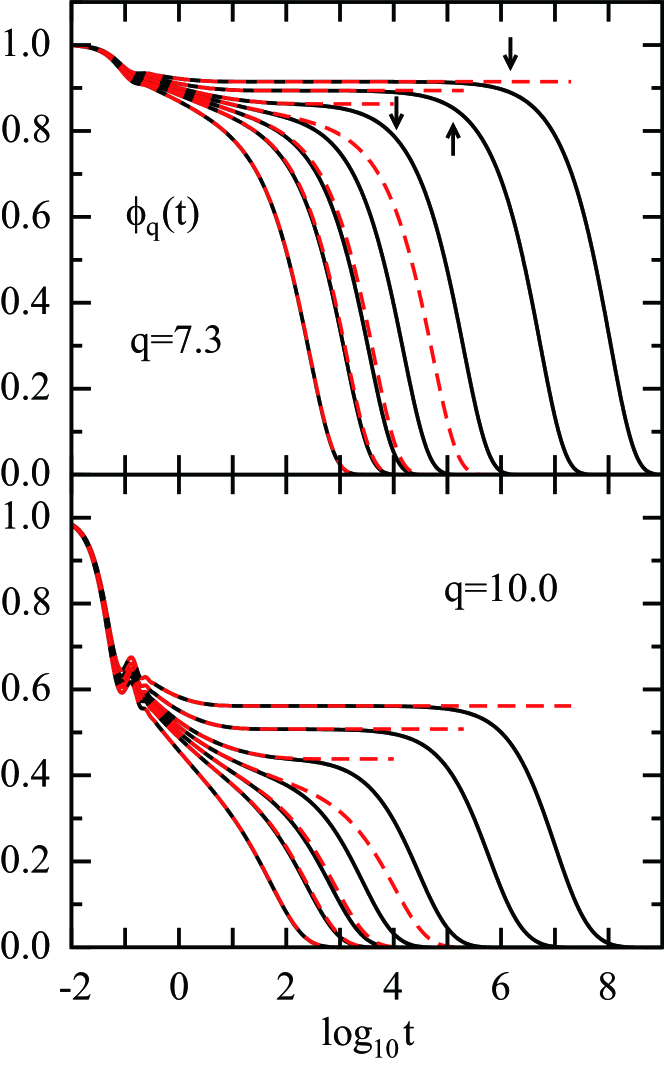
Figure 1: (Color online) Coherent density correlators $\phi_{q}(t)$ as a function of $\log_{10}t$ for reduced temperatures $\epsilon\equiv(T_{\rm c}-T)/T_{\rm c}=-0.10$, $-0.05$, $-0.03$, $-0.01$, $+0.01$, $+0.05$, and $+0.10$ (from left to right). The wave numbers are $q=7.3$ (upper panel) and $q=10.0$ (lower panel), which correspond to the first-peak and first-minimum positions of $S_{q}$, respectively. The solid and dashed curves denote the results from the extended and idealized MCT, respectively. The arrows in the upper panel refer to the peak positions of the non-Gaussian parameter $\alpha_{2}(t)$ for $\epsilon=+0.01$, $+0.05$, and $+0.10$ (cf. Sec. III.3).

Figure 1 shows the coherent density correlators $\phi_{q}(t)$ for representative reduced temperatures $\epsilon\equiv(T_{\rm c}-T)/T_{\rm c}$ whose values are specified in the caption. The wave numbers shown are $q=7.3$ (upper panel) and $q=10.0$ (lower panel), which correspond to the first-peak and first-minimum positions of $S_{q}$, respectively. The dashed curves refer to the idealized-MCT results which exhibit the ergodic ($\epsilon<0$) to nonergodic ($\epsilon\geq 0$) transition at $T=T_{\rm c}$ ($\epsilon=0$) Götze (1991); Franosch et al. (1997). The solid curves denote the results from the extended MCT.

It is seen from Fig. 1 that the solid curves for $\epsilon=-0.10$ and $-0.05$ are hardly affected by the hopping processes, but a slight deviation from the dashed curve is discernible in the $\alpha$-relaxation regime of the solid curve for $\epsilon=-0.03$. The solid curve for $\epsilon=-0.01$ exhibits the same decay up to $\log_{10}t\approx 2$ as the corresponding dashed curve, but the relaxation thereafter is considerably accelerated. The effects from the hopping processes are drastic for $\epsilon>0$ where the idealized MCT predicts the arrested dynamics at the plateau $f_{q}$, whereas the corresponding solid curves from the extended theory relax to zero for long times.

It would be interesting to analyze these extended-MCT results based on various scaling laws developed in Ref. Götze and Sjögren (1987). Such an analysis, however, shall be deferred to subsequent publications, and in the following, we will focus on the connections of the hopping processes with the breakdown of the SE relation and with aspects of dynamical heterogeneities.

III.2 Breakdown of the Stokes-Einstein relation

Here we investigate the breakdown of the SE relation based on the extended MCT, and compare our theoretical prediction with related computer-simulation results and experimental data. A convenient experimental measure of the breakdown is a product $D\eta/T$ formed with the diffusion coefficient $D$ and the viscosity $\eta$, which grows as the SE relation fails Chang and Sillescu (1997). In the present study, the $\alpha$-relaxation time $\tau_{q^{*}}$ of the coherent density correlator at the peak position $q^{*}=7.3$ of $S_{q}$, defined via the convention $\phi_{q^{*}}(\tau_{q^{*}})=0.1$, shall be used as a substitute for $\eta/T$. This is justified since the $T$ dependence of the $\alpha$-relaxation time at the structure factor peak is known to track that of $\eta/T$ Mezei et al. (1987); Yamamoto and Onuki (1998). The diffusion coefficient is determined from the long-time asymptote $D=\lim_{t\to\infty}\delta r^{2}(t)/6t$ of the mean-squared displacement $\delta r^{2}(t)\equiv\langle[{\vec{r}}_{s}(t)-{\vec{r}}_{s}(0)]^{2}\rangle$, whose extended-MCT equations are derived in Appendix B.1.

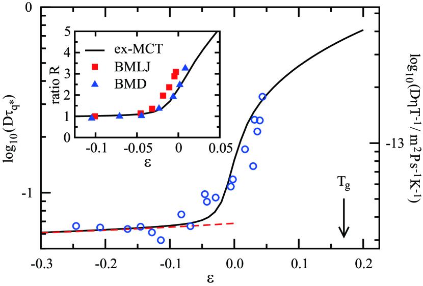
Figure 2: (Color online) Logarithmic representation of the product $D\tau_{q^{*}}$ as a function of the reduced temperature $\epsilon=(T_{\rm c}-T)/T_{\rm c}$. The solid and dashed curves, both referring to the left scale, denote the results from the extended and idealized MCT, respectively. Circles (right scale) denote the $D\eta/T$ data of salol taken from Ref. Chang and Sillescu (1997) and plotted versus $\epsilon$ with $T_{\rm c}=262.7$ K Li et al. (1992). The arrow marks $T_{\rm g}=218$ K of salol. Both the left and right ordinates range over 1.3 decades. The inset exhibits the ratio $R$ of the product $D\tau_{q^{*}}$ to the one at a reference temperature where the SE relation holds. The prediction from the extended MCT (solid curve) is compared with simulation results for a binary mixture of Lennard-Jones particles Kob and Andersen (1994) (filled squares) and a binary mixture of dumbbell molecules of elongation $\zeta=0.8$ Chong et al. (2005) (filled triangles). The procedure for the comparison is detailed in Ref. com (b).

Figure 2 shows the theoretical prediction for the product $D\tau_{q^{*}}$ as a function of the reduced temperature $\epsilon=(T_{\rm c}-T)/T_{\rm c}$. The solid and dashed curves, both referring to the left scale, denote the results from the extended and idealized MCT, respectively. The idealized-MCT result for $D\tau_{q^{*}}$ varies little for $\epsilon<0$ (the increase is only about 10% for the $\epsilon$ range shown in Fig. 2), and does not account for the breakdown of the SE relation. This reflects the universal $\alpha$-scale coupling predicted by the idealized MCT Götze (1991), according to which both the $\alpha$-relaxation time $\tau_{q^{*}}$ and the inverse of the diffusivity $1/D$ exhibit a universal power-law behavior $|\,\epsilon\,|^{-\gamma}$ for small $\epsilon$, and hence, the product $D\tau_{q^{*}}$ approaches a constant for $\epsilon\to 0-$ ($T\to T_{\rm c}+$). On the other hand, the extended MCT predicts the increase of the product $D\tau_{q^{*}}$ for $\epsilon\gtrsim-0.05$. Figure 2 thus shows one of the main results of this paper that the hopping processes are responsible for the breakdown of the SE relation.

Also presented in Fig. 2 is the comparison of the theoretical result with the $D\eta/T$ data of salol taken from Ref. Chang and Sillescu (1997) (circles, right scale). The experimental data are also plotted versus $\epsilon$ with $T_{\rm c}=262.7$ K of salol determined in Ref. Li et al. (1992). A direct comparison between the theoretical result and the experimental data can be made by plotting them on logarithmic scales of the same range as done in Fig. 2. It is seen that the extended-MCT result is consistent with the experimental data concerning the degree of the breakdown of the SE relation.

The inset of Fig. 2 compares the extended-MCT result (solid curve) with simulation results for a binary mixture of Lennard-Jones particles Kob and Andersen (1994) (filled squares) and a binary mixture of dumbbell molecules of elongation $\zeta=0.8$ Chong et al. (2005) (filled triangles). Here the comparison is done in terms of the ratio $R$ of the product $D\tau_{q^{*}}$ to the one at a reference temperature where the SE relation holds. (See Ref. com (b) concerning the details of the comparison.) By definition, the ratio $R$ is unity if the SE relation holds, whereas it exceeds unity as the SE relation fails. Again, the theoretical prediction is consistent with the simulation results.

On the other hand, recent measurements Swallen et al. (2003); Mapes et al. (2006) indicate that the self-diffusion coefficient is about 100 times faster near $T_{\rm g}$ than that predicted by the SE relation. This is about a factor of 10 larger compared to our theoretical prediction near $T_{\rm g}$ (cf. Fig. 2), assuming that $T_{\rm g}$ of the present system is located at $\epsilon\approx 0.17$ estimated from the reduced temperature at $T_{\rm g}$ of salol. This implies that our model for the hopping kernel might be too primitive to be applicable near $T_{\rm g}$. In the following, we shall therefore focus mainly on the regime $\epsilon\lesssim+0.05$ where our theoretical prediction is consistent with the simulation results and experimental data.

III.3 Aspects of dynamical heterogeneities

III.3.1 Non-Gaussian parameter

We next explore a connection of the hopping processes with aspects of dynamical heterogeneities. We start from the discussion on the non-Gaussian parameter $\alpha_{2}(t)$ which characterizes deviations from the Gaussian behavior of the van Hove self correlation function Rahman (1964):

$$\alpha_{2}(t)\equiv\frac{3}{5}\left[\delta r^{4}(t)/\delta r^{2}(t)^{2}\right]-1.$$ (16)

Here $\delta r^{4}(t)\equiv\langle[{\vec{r}}_{s}(t)-{\vec{r}}_{s}(0)]^{4}\rangle$. General properties of $\alpha_{2}(t)$ revealed by computer simulations can be summarized as follows Kob et al. (1997): (i) on the time scale at which the motion of particles is ballistic, $\alpha_{2}(t)$ is zero; (ii) upon entering the time scale of the $\beta$ relaxation where the density correlators are close to their plateaus, $\alpha_{2}(t)$ starts to increase; and (iii) on the time scale of the $\alpha$ relaxation, $\alpha_{2}(t)$ decreases to zero, reflecting diffusive dynamics at long times which is a Gaussian process. It is also observed that the maximum value of $\alpha_{2}(t)$ and the time at which this maximum is attained both increase with decreasing $T$ Kob et al. (1997). Positive $\alpha_{2}(t)$ means that the probability for a particle to move very far is enhanced relative to the one expected for a random-walk process. The peak height of $\alpha_{2}(t)$ has therefore been interpreted as a measure of the dynamical heterogeneity that reflects different local environments around an individual particle.

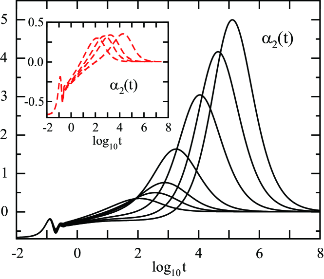
Figure 3: (Color online) Non-Gaussian parameter $\alpha_{2}(t)$ as a function of $\log_{10}t$ based on the extended MCT for reduced temperatures $\epsilon=(T_{\rm c}-T)/T_{\rm c}=-0.10$, $-0.05$, $-0.03$, $-0.01$, $+0.01$, $+0.03$, and $+0.05$ (from left to right). The corresponding results from the idealized MCT, but for $\epsilon<0$ (i.e., $T>T_{\rm c}$) only, are presented as dashed curves in the inset to avoid the overcrowding of the figure. Notice about an order of magnitude difference in the ordinate scales.

The extended-MCT equations for determining the non-Gaussian parameter are derived in Appendix B.2, and the resulting $\alpha_{2}(t)$ are plotted in Fig. 3 for reduced temperatures $\epsilon=(T_{\rm c}-T)/T_{\rm c}$ specified in the caption. The corresponding results from the idealized MCT, but for $\epsilon<0$ (i.e., $T>T_{\rm c}$) only, are presented as dashed curves in the inset to avoid the overcrowding of the figure. As noticed at the end of Appendix B.2, the peculiar behavior $\alpha_{2}(t\to 0)=-2/3$ for short times as predicted by our theory simply reflects that the ideal-gas contribution to the memory kernel is discarded in the mode-coupling approach. Such an ideal-gas contribution is responsible for the short-time ballistic regime, but is irrelevant as far as the long-time dynamics is concerned.

It is seen from the inset of Fig. 3 that the peak height of $\alpha_{2}(t)$ predicted by the idealized MCT does not grow with decreasing $T$, and it is underestimated by almost an order of magnitude compared to that reported in computer simulations Kob et al. (1997). This defect has already been known from the theoretical work in Ref. Fuchs et al. (1998), and has been demonstrated more explicitly in Ref. Flenner and Szamel (2005b). The main panel of Fig. 3, on the other hand, indicates that a substantial improvement is achieved by the extended MCT in that the peak height grows upon lowering $T$ to an extent as observed in simulations Kob et al. (1997). (Notice an order of magnitude difference in the ordinate scales of the main panel and the inset.) Thus, the extended MCT reproduces a feature of the dynamical heterogeneity characterized by the non-Gaussian parameter, and this is accomplished via the inclusion of the hopping processes.

III.3.2 Probability distribution of particle displacements

In terms of the non-Gaussian parameter $\alpha_{2}(t)$, the dynamics is most heterogeneous in the late-$\beta$ or early $\alpha$ regime where the density correlators start to decay from the plateau (see the upper panel of Fig. 1). Recently, it has been recognized from studies of four-point density correlation functions that there exists dynamical heterogeneity on a much longer time scale comparable to the $\alpha$-relaxation time $\tau_{q^{*}}$ Lačević et al. (2003). Recognizing that $\alpha_{2}(t)$ is dominated by those particles which move farther than expected from a Gaussian distribution of particle displacements, Flenner and Szamel introduced a new non-Gaussian parameter $\gamma(t)\equiv(1/3)\delta r^{2}(t)[\delta r^{2}]^{-1}(t)-1$ with $[\delta r^{2}]^{-1}(t)\equiv\langle 1/[{\vec{r}}_{s}(t)-{\vec{r}}_{s}(0)]^{2}\rangle$, which weights strongly the particles which have not moved as far as expected from the Gaussian distribution Flenner and Szamel (2005a). It is found that the peak position of $\gamma(t)$ is located on the time scale of $\tau_{q^{*}}$, and hence, characterizes the longer-time dynamical heterogeneity. It is also observed that the peak position of $\gamma(t)$ corresponds to the time at which two peaks in the probability distribution of particle displacements, reflecting populations of mobile and immobile particles (see below), are of equal height. This implies that the presence of the longer-time dynamical heterogeneity can be examined also through such a probability distribution.

The mentioned probability distribution $P(\log_{10}(\delta r);t)$ of the logarithm of particle displacements $\delta r$ at time $t$ can be obtained from the van Hove self correlation function $G_{s}(\delta r,t)$ by the transformation Flenner and Szamel (2005a)

$$P(\log_{10}(\delta r);t)=\ln(10)\,4\pi\delta r^{3}G_{s}(\delta r,t).$$ (17)

The probability distribution is defined such that the integral $\int_{x_{0}}^{x_{1}}dx\,P(x;t)$ is the fraction of particles whose value of $\log_{10}(\delta r)$ is between $x_{0}$ and $x_{1}$. If the motion of a particle is diffusive with a diffusion coefficient $D$, there holds $G_{s}(\delta r,t)\approx[1/(4\pi Dt)^{3/2}]\exp(-\delta r^{2}/4Dt)$ Hansen and McDonald (1986). As argued in Ref. Flenner and Szamel (2005a), the shape of the corresponding probability distribution under the diffusion approximation becomes time independent with the peak height $\approx 2.13$.

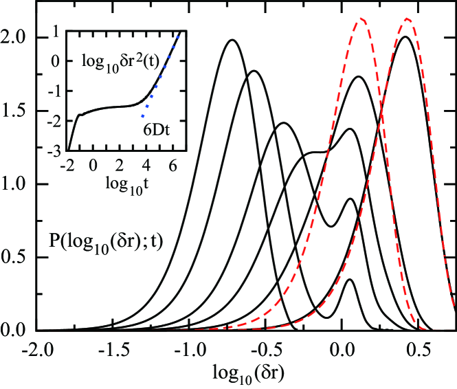
Figure 4: Probability distribution $P(\log_{10}(\delta r);t)$ of the logarithm of single particle displacements based on the extended MCT at the reduced temperature $\epsilon=(T_{\rm c}-T)/T_{\rm c}=+0.01$ (solid curves). The times shown are $t=5.4\times 10^{3}$, $4.3\times 10^{4}$, $1.7\times 10^{5}$, $3.4\times 10^{5}$, $6.8\times 10^{5}$, and $2.7\times 10^{6}$ (from left to right). The $\alpha$-relaxation time $\tau_{q^{*}}$ at this reduced temperature is $\tau_{q^{*}}=4.3\times 10^{5}$ (cf. Fig. 1). The dashed curves refer to the probability distribution under the diffusion approximation for $t=6.8\times 10^{5}$ and $2.7\times 10^{6}$. The inset exhibits the time evolution of the mean-squared displacement $\delta r^{2}(t)$ at $\epsilon=+0.01$ on double logarithmic scales (solid curve). The dotted curve refers to the diffusion asymptote, $6Dt$.

Figure 4 shows the extended-MCT result for the probability distribution $P(\log_{10}(\delta r);t)$ (solid curves) at the reduced temperature $\epsilon=(T_{\rm c}-T)/T_{\rm c}=+0.01$. The times shown are $t=5.4\times 10^{3}$, $4.3\times 10^{4}$, $1.7\times 10^{5}$, $3.4\times 10^{5}$, $6.8\times 10^{5}$, and $2.7\times 10^{6}$. The $\alpha$-relaxation time $\tau_{q^{*}}$ at this reduced temperature is $\tau_{q^{*}}=4.3\times 10^{5}$ (cf. Fig. 1). The dashed curves refer to the probability distribution under the diffusion approximation for $t=6.8\times 10^{5}$ and $2.7\times 10^{6}$. The inset exhibits the mean-squared displacement $\delta r^{2}(t)$ at $\epsilon=+0.01$ on double logarithmic scales, from which one understands that the times chosen in the main panel range from the late-$\beta$, plateau regime to the final $\alpha$ regime where $\delta r^{2}(t)\sim 6Dt$.

The appearance of the plateau in $\delta r^{2}(t)$ is due to particles being caged Fuchs et al. (1998), and the peak of the probability distribution $P(\log_{10}(\delta r);t)$ for $t=5.4\times 10^{3}$ reflects populations of such “immobile” particles. At later times, the second peak develops in the probability distribution at $\log_{10}(\delta r)\approx 0.0$ (i.e., $\delta r\approx 1.0$), reflecting “mobile” particles hopping over interparticle distances. One infers from Fig. 4 that the time at which the two peaks in $P(\log_{10}(\delta r);t)$ become of equal height is located on the time scale of $\tau_{q^{*}}$, and this is consistent with the simulation result Flenner and Szamel (2005a). Subsequently, the double-peak structure disappears, and the probability distribution approaches the one well described by the diffusion approximation.

Coexistence of mobile and immobile particles is a direct indication of the dynamical heterogeneity Ediger (2000). Our results shown in Fig. 4 indicate that the hopping processes are responsible for such a double-peak structure in the probability distribution $P(\log_{10}(\delta r);t)$ occurring on the time scale $\tau_{q^{*}}$ of the $\alpha$ relaxation. This also explains why the idealized MCT failed to reproduce the double-peak structure in $P(\log_{10}(\delta r);t)$ Flenner and Szamel (2005b).

III.3.3 Growing dynamic length scale

Figure 4 also implies that the probability distribution approaches its diffusion asymptote only after its peak position exceeds those length scales where the double-peak structure in $P(\log_{10}(\delta r);t)$ is observable. Thus, there is a certain length scale above which Fickian diffusion sets in. In the following, we shall quantify such a length scale characterizing the crossover from non-Fickian to Fickian diffusion, and investigate its temperature dependence.

To this end, let us introduce the ratio $R_{q}^{s}$ of the product $q^{2}D\tau_{q}^{s}$ to the one at some reference temperature, which is an analogue of the ratio $R$ studied in the inset of Fig. 2. Here the $\alpha$-relaxation time $\tau_{q}^{s}$ of the tagged-particle density correlator is defined via the convention $\phi_{q}^{s}(\tau_{q}^{s})=0.1$. Under the diffusion approximation, there holds $\phi_{q}^{s}(t)\approx\exp(-q^{2}Dt)$ Hansen and McDonald (1986). Thus, the product $q^{2}D\tau_{q}^{s}$ is constant, and hence, the ratio $R_{q}^{s}$ is unity, if the dynamics on the length scale $\approx 2\pi/q$ is diffusive. On the other hand, the ratio $R_{q}^{s}$ exceeds unity if the dynamics on the length scale $\approx 2\pi/q$ is non-Fickian. We shall therefore define the crossover wave number $q_{\rm onset}$ via $R_{q_{\rm onset}}^{s}=1.1$, i.e., as the wave number at which the ratio $R_{q}^{s}$ reaches 10% above unity. The onset length scale of Fickian diffusion shall then be defined via $\ell_{\rm onset}\equiv 2\pi/q_{\rm onset}$.

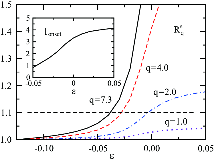
Figure 5: (Color online) Ratio $R_{q}^{s}$ of the product $q^{2}D\tau_{q}^{s}$ to the one at a reference temperature $T_{\rm ref}$ as a function of the reduced temperature $\epsilon=(T_{\rm c}-T)/T_{\rm c}$. Here $T_{\rm ref}$ is chosen such that $(T_{\rm c}-T_{\rm ref})/T_{\rm c}=-0.125$. The wave numbers shown are $q=7.3$ (solid curve), 4.0 (dashed curve), 2.0 (dashed-dotted curve), and 1.0 (dotted curve). The horizontal dashed line marks $R_{q}^{s}=1.1$ chosen to determine the crossover wave number $q_{\rm onset}$ introduced in the text. The inset exhibits the onset length scale of Fickian diffusion $\ell_{\rm onset}\equiv 2\pi/q_{\rm onset}$ as a function of the reduced temperature $\epsilon$.

Figure 5 exhibits the ratio $R_{q}^{s}$ for wave numbers $q=7.3$ (solid curve), 4.0 (dashed curve), 2.0 (dashed-dotted curve), and 1.0 (dotted curve), as a function of the reduced temperature $\epsilon=(T_{\rm c}-T)/T_{\rm c}$. The reference temperature $T_{\rm ref}$ for calculating $R_{q}^{s}$ is chosen such that $(T_{\rm c}-T_{\rm ref})/T_{\rm c}=-0.125$. The horizontal dashed line marks $R_{q}^{s}=1.1$ chosen to determine the crossover wave number $q_{\rm onset}$ introduced above.

For reduced temperatures $\epsilon\lesssim-0.04$, all the ratios $R_{q}^{s}$ shown in Fig. 5 are less than 1.1, implying that the tagged-particle dynamics on the length scales comparable to and larger than $2\pi/7.3\approx 0.86$ can be well described by the Fickian diffusion law. For $\epsilon>-0.04$, $R_{q}^{s}$ for $q=7.3$ exceeds 1.1, meaning that the dynamics is diffusive only on length scales larger than 0.86. The onset length scale $\ell_{\rm onset}$ of Fickian diffusion increases to $2\pi/4.0\approx 1.6$ at $\epsilon\approx-0.03$, and to $2\pi/2.0\approx 3.1$ at $\epsilon\approx 0$, as can be inferred from Fig. 5. The length scale $\ell_{\rm onset}$ so obtained as a function of the reduced temperature $\epsilon$ is summarized in the inset of Fig. 5. Thus, the extended MCT predicts the presence of a growing dynamic length scale. It is anticipated that $\ell_{\rm onset}$ is intimately related to the mean size of the dynamic clusters observed in simulations Berthier (2004), since Fickian diffusion, i.e., a random-walk process, is possible only over those length scales where the coherence length of such clusters is smeared out.

IV Summary

In this paper, we developed a new extended version of MCT for glass transition. The activated hopping processes are incorporated via the dynamical theory, originally formulated to describe diffusion-jump processes in crystals and adapted in this work to glass-forming liquids. The dynamical-theory approach treats hopping as arising from vibrational fluctuations in quasi-arrested state where particles are trapped inside their cages, and the hopping rate is formulated in terms of the Debye-Waller factors characterizing the structure of the quasi-arrested state. The resulting expression for the hopping rate takes an activated form, and the barrier height for the hopping is “self-generated” in the sense that it is present only in those states where the dynamics exhibits a well defined plateau. It is discussed how such a hopping rate can be incorporated to develop a new extended MCT.

The extended MCT deals with the interplay of two effects. Nonlinear interactions of density fluctuations, as described by the idealized memory kernel $m_{q}^{\rm id}(z)$, lead to the cage effect with a trend to produce arrested states for sufficiently low temperatures. Phonon assisted hoppings, taken into account via the hopping kernel $\delta_{q}(z)$, lead to the $\alpha$ relaxation at all temperatures and restore ergodicity. The interplay of these two effects is described by the memory kernel $m_{q}(z)$ via Eq. (3b) which has the form of a Dyson equation. As demonstrated in Sec. III for a model of the Lennard-Jones system, it leads to nontrivial theoretical predictions concerning the breakdown of the SE relation and characteristic features of dynamical heterogeneities, which the idealized version of the theory failed to reproduce.

In dense liquids, relaxation is necessarily connected with rearrangements of large complexes of particles. We have seen in Fig. 3 that the peak height of the non-Gaussian parameter $\alpha_{2}(t)$ grows substantially in the late-$\beta$ regime as the temperature is decreased. This enhanced probability for a particle to move further is what one would expect as a result of the building of a backflow in the liquid, and it is anticipated that the string-like motions observed in the late-$\beta$ regime Donati et al. (1998) reflect such a backflow pattern. The backflow was originally discussed by Feynman and Cohen and taken into account in their theory for roton spectrum in liquid helium Feynman and Cohen (1956). Subsequently, it was found that the quantum-mechanical analogue of the idealized memory kernel reproduces the Feynman-Cohen result for roton spectrum Götze and Lücke (1976), i.e., the backflow phenomenon is within the scope of the idealized MCT Götze and Sjögren (1995). However, the idealized memory kernel alone does not account for such a pronounced peak in $\alpha_{2}(t)$ as observed in computer simulations Fuchs et al. (1998). This implies that the mentioned interplay with the hopping kernel plays a relevant role for the substantial increase of $\alpha_{2}(t)$ and the building of the backflow.

The double-peak structure in the probability distribution $P(\log_{10}(\delta r);t)$ of particle displacements, which is most pronounced on the time scale $\tau_{q^{*}}$ of the $\alpha$-relaxation and disappears at longer times (cf. Fig. 4), reflects coexistence of mobile and immobile particles with a life time $\approx\tau_{q^{*}}$, and is a direct indication of the dynamical heterogeneity Ediger (2000). The extended MCT developed here provides a natural explanation for its origin in terms of the cage and hopping effects. As argued in Sec. III.3.3, the life time of the double-peak structure gives rise to a growing dynamic length scale $\ell_{\rm onset}$, which is associated with the decoupling of the time scales of the $\alpha$ processes occurring on length scales smaller than $\ell_{\rm onset}$ from the diffusion coefficient. The breakdown of the SE relation discussed in Sec. III.2 can also be understood in terms of the decoupling of the $\alpha$-relaxation time $\tau_{q^{*}}$ from the diffusivity which occurs when $\ell_{\rm onset}$ exceeds the average interparticle distance $\approx 2\pi/q^{*}$. It is anticipated that the onset length scale $\ell_{\rm onset}$ of Fickian diffusion is intimately related to the mean size of the dynamic clusters observed in simulations Berthier (2004), since Fickian diffusion, i.e., a random-walk process, is possible only over those length scales where the coherence length of such clusters is smeared out. Then, our picture for the breakdown of the SE relation is consistent with that of Ref. Berthier (2004), where the connection between decoupling phenomena and the growing coherence length scale is discussed.

It is certainly necessary to improve further the theory developed here. First of all, possible correlated hopping effects are discarded in our model for the hopping kernel. This might explain why our theory underestimates the degree of the breakdown of the SE relation near $T_{\rm g}$, which we referred to in connection with Fig. 2. That the development of the length scale $\ell_{\rm onset}$ seems suppressed for $\epsilon>0$, as can be inferred from the inset of Fig. 5, might also be related to such a defect of the present theory. Second, we did not determine $\Delta^{2}$ – a square of the ratio $\Delta=x^{*}/a$ formed with the critical size $x^{*}$ of the phonon-assisted fluctuation needed to cause a hopping and the average interparticle distance $a$ (cf. Sec. II) – microscopically, but simply took a value ($\Delta^{2}=0.10$) from the literature. Regarding this, let us mention that nearly the same results as those presented in Sec. III can be obtained with other values of $\Delta^{2}$, as far as those values consistent with the Lindemann length com (a) are chosen. Thus, our theoretical results do not rely on the specific value of $\Delta^{2}=0.10$. But, of course, it is desirable to determine $\Delta^{2}$ consistently within the theory. Third, the $\alpha$-relaxation stretching is not enhanced at low temperatures. For example, the stretching exponents $\beta_{q}$, obtained via Kohlrausch-law fits of the density correlators shown in Fig. 1, for $q=10.0$ are 0.76, 0.79, and 0.80 for $\epsilon=+0.01$, $+0.05$, and $+0.10$, respectively. One possibility to overcome this defect is to take into account distribution of hopping rates or barrier heights, which can be done, e.g., by considering fluctuations in the Debye-Waller factors and $\Delta^{2}$. Four-point density correlators might be necessary for this purpose, though it is a difficult task to calculate such higher-order correlators. But, in view of the significant results achieved by our theory, it is promising to pursue its further development.

Appendix A Novel derivation of the hopping kernel of Götze and Sjögren

In order to go beyond the idealized MCT, one has to consider corrections to the idealized memory kernel, $m_{q}(z)=m_{q}^{\rm id}(z)+\Delta m_{q}(z)$. The extended MCT of Götze and Sjögren Götze and Sjögren (1987, 1995) can be considered as a theory for such corrections, and yields an expression for $\Delta m_{q}(z)$ in terms of the hopping kernel $\delta_{q}(z)$ that involves couplings to currents. Their extended theory is formulated with the generalized kinetic theory for phase-space density fluctuations, but essentially the same expression for the hopping kernel $\delta_{q}(z)$ can be derived also with the standard projection-operator approach based on density and current-density fluctuations. In this appendix, we outline such a novel derivation.

We start from reviewing the derivation of the idealized memory kernel $m_{q}^{\rm id}(t)$ (see Ref. Götze (1991) for details). Let us introduce a projection operator ${\cal P}$ onto the subspace spanned by the density fluctuations $\rho_{\vec{q}}$ and the current-density fluctuations $j_{\vec{q}}^{\lambda}\equiv\sum_{i}v_{i}^{\lambda}\exp(i{\vec{q}}\cdot{\vec{r}}_{i})$ ($\lambda=x,y,z$). Here $v_{i}^{\lambda}$ denotes the $\lambda$ component of the velocity of $i$th particle. Within the Zwanzig-Mori formalism Hansen and McDonald (1986), one obtains based on the operator ${\cal P}$ the exact equation (1a) for the coherent density correlator $\phi_{q}(t)$. The formal expression for the memory kernel entering there reads

$$\Omega_{q}^{2}m_{q}(t)=\frac{M}{Nk_{\rm B}T}\langle F_{\vec{q}}^{*}e^{i{\cal QLQ}t}F_{\vec{q}}\rangle,$$ (18)

where ${\cal Q}\equiv 1-{\cal P}$, and the fluctuating force is given by

$$F_{\vec{q}}=\partial_{t}(\hat{\vec{q}}\cdot{\vec{j}}_{\vec{q}})-iq\frac{k_{\rm B}T}{MS_{q}}\rho_{\vec{q}}.$$ (19)

Here $\hat{\vec{q}}={\vec{q}}/q$. Under the mode-coupling approach, the fluctuating forces are approximated by their projections onto the subspace spanned by pair-density modes $\rho_{\vec{k}}\rho_{\vec{p}}$; this is done by introducing the second projection operator

$${\cal P}_{2}X=\sum_{{\vec{k}}>{\vec{p}}}\rho_{\vec{k}}\rho_{\vec{p}}\,\frac{1}{N^{2}S_{k}S_{p}}\,\langle\rho_{\vec{k}}^{*}\rho_{\vec{p}}^{*}X\rangle,$$ (20)

and approximating $F_{\vec{q}}\approx{\cal P}_{2}F_{\vec{q}}\equiv F_{\vec{q}}^{\rho\rho}$, i.e.,

$$\Omega_{q}^{2}m_{q}(t)\approx\frac{M}{Nk_{\rm B}T}\langle F_{\vec{q}}^{\rho\rho\,*}e^{i{\cal QLQ}t}F_{\vec{q}}^{\rho\rho}\rangle.$$ (21)

Notice here that the static factorization approximation

$$\langle\rho_{\vec{k}}^{*}\rho_{\vec{p}}^{*}\rho_{{\vec{k}}^{\prime}}\rho_{{\vec{p}}^{\prime}}\rangle\approx\delta_{{\vec{k}},{\vec{k}}^{\prime}}\delta_{{\vec{p}},{\vec{p}}^{\prime}}N^{2}S_{k}S_{p}\,\,\,({\vec{k}}>{\vec{p}},{\vec{k}}^{\prime}>{\vec{p}}^{\,\prime}),$$ (22)

is already used in the definition (20) of ${\cal P}_{2}$. Within the convolution approximation for triple density correlations, one finds for the projected fluctuating force

$$F_{\vec{q}}^{\rho\rho} = -i\frac{\rho k_{\rm B}T}{NM}\sum_{{\vec{k}}>{\vec{p}}}\delta_{{\vec{q}},{\vec{k}}+{\vec{p}}}$$ (23a)

$$\qquad\qquad\times\,(\hat{\vec{q}}\cdot{\vec{k}}\,c_{k}+\hat{\vec{q}}\cdot{\vec{p}}\,c_{p})\rho_{\vec{k}}\rho_{\vec{p}}$$

$$= -i\frac{\rho k_{\rm B}T}{NM}\sum_{\vec{k}}\hat{\vec{q}}\cdot{\vec{k}}\,c_{k}\rho_{\vec{k}}\rho_{{\vec{q}}-{\vec{k}}}.$$ (23b)

Substituting Eq. (23a) into Eq. (21) and then using the dynamical factorization approximation

$$\langle\rho_{\vec{k}}^{*}\rho_{\vec{p}}^{*}\,e^{i{\cal QLQ}t}\rho_{{\vec{k}}^{\prime}}\rho_{{\vec{p}}^{\prime}}\rangle\approx\delta_{{\vec{k}},{\vec{k}}^{\prime}}\delta_{{\vec{p}},{\vec{p}}^{\prime}}N^{2}S_{k}S_{p}\phi_{k}(t)\phi_{p}(t)$$

$$\qquad\qquad\qquad\qquad\qquad\qquad({\vec{k}}>{\vec{p}},{\vec{k}}^{\prime}>{\vec{p}}^{\,\prime}),$$ (24)

which factorizes averages of products evolving in time with the generator ${\cal QLQ}$ into products of averages formed with variables evolving with ${\cal L}$, one obtains the idealized kernel $m_{q}^{\rm id}(t)$ given in Eqs. (2).

To extend the idealized theory, one has to avoid the use of the dynamical factorization approximation (24). We shall therefore start from Eqs. (21) and (23b) for the memory kernel $m_{q}(t)$, to which the approximation (24) has yet to be applied. Notice, however, that the static factorization approximation (22) is still assumed in our approach; this is employed in the definition (20) of ${\cal P}_{2}$, which is then used in deriving Eq. (23b). Thus, there holds $m_{q}(0)=m_{q}^{\rm id}(0)$ at $t=0$.

By introducing a new projection operator ${\cal P}^{\prime}$ onto the subspace spanned by $F_{\vec{q}}^{\rho\rho}$, i.e.,

$${\cal P}^{\prime}X=F_{\vec{q}}^{\rho\rho}\frac{M}{Nk_{\rm B}T\,\Omega_{q}^{2}m_{q}(0)}\langle F_{\vec{q}}^{\rho\rho\,*}X\rangle,$$ (25)

one obtains the following Zwanzig-Mori equation of motion for $m_{q}(t)$:

$$\partial_{t}m_{q}(t)+m_{q}(0)\int_{0}^{t}dt^{\prime}\,L_{q}(t-t^{\prime})m_{q}(t^{\prime})=0.$$ (26)

Here the factor $m_{q}(0)$ in front of the convolution integral is just for later convenience, and the formal expression for the “memory kernel” $L_{q}(t)$ is given by

$$m_{q}(0)L_{q}(t)=\frac{M}{Nk_{\rm B}T\,\Omega_{q}^{2}m_{q}(0)}\langle R_{\vec{q}}^{*}\,e^{i{\cal Q}^{\prime}{\cal QLQ}{\cal Q}^{\prime}t}\,R_{\vec{q}}\rangle,$$ (27)

in terms of the “fluctuating force”

$$R_{\vec{q}}=i{\cal Q}^{\prime}{\cal QLQ}F_{\vec{q}}^{\rho\rho},$$ (28)

where we have introduced ${\cal Q}^{\prime}\equiv 1-{\cal P}^{\prime}$. Substituting Eq. (23b) into Eq. (28), one finds

$$R_{\vec{q}} = \frac{\rho k_{\rm B}T}{NM}\sum_{\vec{k}}\hat{\vec{q}}\cdot{\vec{k}}\,c_{k}\bigl{\{}{\vec{k}}\cdot{\vec{j}}_{\vec{k}}\,\rho_{\vec{p}}+{\vec{p}}\cdot{\vec{j}}_{\vec{p}}\,\rho_{\vec{k}}$$ (29)

$$\qquad\qquad\quad-\,({\vec{k}}\cdot{\vec{j}}_{\vec{q}}\,S_{p}+{\vec{p}}\cdot{\vec{j}}_{\vec{q}}\,S_{k})\bigr{\}},$$

in which ${\vec{p}}={\vec{q}}-{\vec{k}}$.

Now, we apply the mode-coupling approximation to the kernel $L_{q}(t)$. Because of the odd time reversal symmetry of $R_{\vec{q}}$, the simplest mode-coupling approximation for $L_{q}(t)$ can be introduced by defining the projection operator ${\cal P}_{2}^{\prime}$ onto the subspace panned by the product $\rho_{\vec{k}}j_{\vec{p}}^{\lambda}$ of the density and current-density modes:

$${\cal P}_{2}^{\prime}X=\sum_{\vec{k}}\sum_{\lambda}\rho_{\vec{k}}j_{\vec{p}}^{\lambda}\,\frac{M}{N^{2}k_{\rm B}T\,S_{k}}\,\langle\rho_{\vec{k}}^{*}j_{\vec{p}}^{\lambda\,*}X\rangle,$$ (30)

where we have used the factorization approximation

$$\langle\rho_{\vec{k}}^{*}j_{\vec{p}}^{\lambda\,*}\rho_{{\vec{k}}^{\prime}}j_{{\vec{p}}^{\prime}}^{\mu}\rangle\approx\delta_{{\vec{k}},{\vec{k}}^{\prime}}\delta_{\lambda\mu}N^{2}k_{\rm B}TS_{k}/M.$$ (31)

Here and in the following, we use abbreviations ${\vec{p}}\equiv{\vec{q}}-{\vec{k}}$ and ${\vec{p}}^{\,\prime}\equiv{\vec{q}}-{\vec{k}}^{\prime}$. We thus obtain under the mode-coupling approximation $R_{\vec{q}}\approx{\cal P}_{2}^{\prime}R_{\vec{q}}\equiv R_{\vec{q}}^{\rho j}$,

$$m_{q}(0)L_{q}(t)\approx\frac{M}{Nk_{\rm B}T\,\Omega_{q}^{2}m_{q}(0)}\langle R_{\vec{q}}^{\rho j\,*}e^{i{\cal Q}^{\prime}{\cal QLQ}{\cal Q}^{\prime}t}R_{\vec{q}}^{\rho j}\rangle.$$ (32)

Within the convolution approximation for triple density correlations, one finds

$$R_{\vec{q}}^{\rho j}=\frac{\rho k_{\rm B}T}{NM}\sum_{\vec{k}}\sum_{\lambda}V_{\lambda}({\vec{q}};{\vec{k}},{\vec{p}}\,)\,\rho_{\vec{k}}j_{\vec{p}}^{\lambda},$$ (33a)

in which $$V_{\lambda}$$ is given by

$$V_{\lambda}({\vec{q}};{\vec{k}},{\vec{p}}\,)=\frac{1}{(2\pi)^{3}}\int d{\vec{k}}^{\prime}\,\hat{\vec{q}}\cdot{\vec{k}}^{\prime}\,c_{k^{\prime}}$$

$$\qquad\quad\times\,(k_{\lambda}^{\prime}S_{p^{\prime}}h_{|{\vec{p}}^{\prime}-{\vec{k}}|}+p_{\lambda}^{\prime}S_{k^{\prime}}h_{|{\vec{k}}^{\prime}-{\vec{k}}|}).$$ (33b)

Here $k_{\lambda}$ refers to the $\lambda$ component of the vector ${\vec{k}}$, and the function $h_{q}$ is given by $h_{q}=c_{q}S_{q}$. When Eq. (33a) is substituted into Eq. (32), the kernel $L_{q}(t)$ is expressed in terms of four-mode correlators, for which we invoke the following dynamical factorization approximation:

$$\langle\rho_{\vec{k}}^{*}j_{\vec{p}}^{\lambda\,*}e^{i{\cal Q}^{\prime}{\cal QLQ}{\cal Q}^{\prime}t}\rho_{{\vec{k}}^{\prime}}j_{{\vec{p}}^{\prime}}^{\mu}\rangle$$

$$\approx\delta_{{\vec{k}},{\vec{k}}^{\prime}}\langle\rho_{\vec{k}}^{*}e^{i{\cal L}t}\rho_{\vec{k}}\rangle\langle j_{\vec{p}}^{\lambda\,*}e^{i{\cal L}t}j_{\vec{p}}^{\mu}\rangle$$

$$\quad+\,\delta_{{\vec{k}},{\vec{p}}^{\prime}}\langle\rho_{\vec{k}}^{*}e^{i{\cal L}t}j_{\vec{k}}^{\mu}\rangle\langle j_{\vec{p}}^{\lambda\,*}e^{i{\cal L}t}\rho_{\vec{p}}\rangle$$

$$=\delta_{{\vec{k}},{\vec{k}}^{\prime}}N^{2}(k_{\rm B}T/M)S_{k}\phi_{k}(t)$$

$$\quad\qquad\times\,[\hat{p}_{\lambda}\hat{p}_{\mu}\phi_{p}^{\rm L}(t)+(\delta_{\lambda\mu}-\hat{p}_{\lambda}\hat{p}_{\mu})\phi_{p}^{\rm T}(t)]$$

$$\quad-\,\delta_{{\vec{k}},{\vec{p}}^{\prime}}N^{2}S_{k}S_{p}(\hat{k}_{\mu}\hat{p}_{\lambda}/kp)\partial_{t}\phi_{k}(t)\partial_{t}\phi_{p}(t).$$ (34)

Here $\phi_{q}^{\rm L}(t)$ and $\phi_{q}^{\rm T}(t)$ are longitudinal and transversal current correlators, respectively, which are normalized to unity at $t=0$. We then obtain the following form for the kernel $L_{q}(t)$ that involves couplings to current modes:

$$L_{q}(t) = \int d{\vec{k}}\,\bigl{[}V_{\rm L}({\vec{q}};{\vec{k}},{\vec{p}}\,)\phi_{k}(t)\phi_{p}^{\rm L}(t)$$ (35a)

$$\quad+\,V_{\rm T}({\vec{q}};{\vec{k}},{\vec{p}}\,)\phi_{k}(t)\phi_{p}^{\rm T}(t)$$

$$\quad+\,V^{\prime}({\vec{q}};{\vec{k}},{\vec{p}}\,)\partial_{t}\phi_{k}(t)\,\partial_{t}\phi_{p}(t)\bigr{]}.$$

The vertex functions $$V_{\rm L} V_{\rm T} V^{\prime} V_{\lambda}$$, , and are expressed in terms of the thermal velocity, the static equilibrium quantities, and given in Eq. (33b) as

$$V_{\rm L}({\vec{q}};{\vec{k}},{\vec{p}}\,)=\frac{\rho k_{\rm B}T}{(2\pi)^{3}M}\frac{S_{q}S_{k}}{q^{2}m_{q}(0)^{2}}\Bigl{[}\sum_{\lambda}\hat{p}_{\lambda}V_{\lambda}({\vec{q}};{\vec{k}},{\vec{p}}\,)\Bigr{]}^{2},$$ (35b)

$$V_{\rm T}({\vec{q}};{\vec{k}},{\vec{p}}\,) = \frac{\rho k_{\rm B}T}{(2\pi)^{3}M}\frac{S_{q}S_{k}}{q^{2}m_{q}(0)^{2}}\Bigl{\{}\sum_{\lambda}V_{\lambda}({\vec{q}};{\vec{k}},{\vec{p}}\,)^{2}$$ (35c)

$$\qquad-\,\Bigl{[}\sum_{\lambda}\hat{p}_{\lambda}V_{\lambda}({\vec{q}};{\vec{k}},{\vec{p}}\,)\Bigr{]}^{2}\Bigr{\}},$$

$$V^{\prime}({\vec{q}};{\vec{k}},{\vec{p}}\,) = -\frac{\rho}{(2\pi)^{3}}\frac{S_{q}S_{k}S_{p}}{q^{2}m_{q}(0)^{2}}\Bigl{[}\sum_{\lambda}\frac{\hat{k}_{\lambda}}{k}V_{\lambda}({\vec{q}};{\vec{p}},{\vec{k}}\,)\Bigr{]}$$ (35d)

$$\qquad\times\,\Bigl{[}\sum_{\lambda}\frac{\hat{p}_{\lambda}}{p}V_{\lambda}({\vec{q}};{\vec{k}},{\vec{p}}\,)\Bigr{]}.$$

Finally, let us connect the Laplace transform of $L_{q}(t)$ to the hopping kernel $\delta_{q}(z)$ using the definition given by Eq. (3a). The Laplace transform of Eq. (26) reads

$$m_{q}(z)=-\frac{m_{q}(0)}{z+m_{q}(0)L_{q}(z)}.$$ (36)

In view of this expression, let us formally introduce the function $L_{q}^{\rm id}(z)$ in terms of the Laplace transform of the idealized memory kernel $m_{q}^{\rm id}(z)$ via

$$m_{q}^{\rm id}(z)=-\frac{m_{q}(0)}{z+m_{q}(0)L_{q}^{\rm id}(z)}.$$ (37)

Here we have used the equality $m_{q}(0)=m_{q}^{\rm id}(0)$ at $t=0$ noticed above. Substituting Eqs. (36) and (37) into Eq. (3a), one obtains for the hopping kernel

$$\delta_{q}(z)=L_{q}(z)-L_{q}^{\rm id}(z).$$ (38)

From the functional form of $L_{q}(t)$ given in Eq. (35a) and interpreting that $L_{q}^{\rm id}(z)$ in Eq. (38) subtracts those contributions already accounted for by the idealized memory kernel $m_{q}^{\rm id}(z)$, one understands that the expression (38) for the hopping kernel is essentially the same as the one derived by Götze and Sjögren Götze and Sjögren (1987, 1995).

Appendix B Extended MCT equations for the mean-squared displacement and the non-Gaussian parameter

B.1 Mean-squared displacement

The equation of motion for the mean-squared displacement $\delta r^{2}(t)$ can be obtained from Eq. (1a) for $\phi_{q}^{s}(t)$ by exploiting its relation to the small-$q$ behavior of $\phi_{q}^{s}(t)=1-q^{2}\delta r^{2}(t)/6+O(q^{4})$ Hansen and McDonald (1986):

$$\partial_{t}\delta r^{2}(t)+\frac{k_{\rm B}T}{M}\int_{0}^{t}dt^{\prime}\,m_{(0)}^{s}(t-t^{\prime})\,\delta r^{2}(t^{\prime})=6\frac{k_{\rm B}T}{M}t.$$ (39)

Here we have introduced the $q\to 0$ limit of the memory kernel via $m_{(0)}^{s}(t)\equiv\lim_{q\to 0}q^{2}m_{q}^{s}(t)$. To obtain $m_{(0)}^{s}(t)$, it is more convenient to rewrite Eq. (3b) in the form

$$m_{q}^{s}(z)=m_{q}^{s\,{\rm id}}(z)+m_{q}^{s\,{\rm id}}(z)\,\delta_{q}^{s}(z)\,m_{q}^{s}(z),$$ (40)

from which one finds

$$m_{(0)}^{s}(z)=m_{(0)}^{s\,{\rm id}}(z)+m_{(0)}^{s\,{\rm id}}(z)\,\delta_{(0)}^{s}(z)\,m_{(0)}^{s}(z).$$ (41a)

Here $$m_{(0)}^{s\,{\rm id}}(z) q\to 0 \delta_{(0)}^{s}(z) \delta_{(0)}^{s}(z)\equiv\lim_{q\to 0}\delta_{q}^{s}(z)/q^{2}$$ refers to the corresponding limit of the idealized memory kernel, and is defined via . The former is given by Fuchs et al. (1998)

$$m_{(0)}^{s\,{\rm id}}(t)=\frac{1}{6\pi^{2}}\int dk\,k^{4}\rho S_{k}c_{k}^{2}\phi_{k}(t)\phi_{k}^{s}(t),$$ (41b)

whereas the latter reads after carrying out the $$q\to 0$$ limit in Eq. (14)

$$\delta_{(0)}^{s}(z)=i\,w_{\rm hop}N_{\rm c}a^{2}/6.$$ (41c)

Equations (39) and (41) constitute the extended-MCT equations for the mean-squared displacement $\delta r^{2}(t)$.

B.2 Non-Gaussian parameter

The non-Gaussian parameter $\alpha_{2}(t)$ defined in Eq. (16) can be obtained from the mean-squared displacement $\delta r^{2}(t)$ and the mean-quartic displacement $\delta r^{4}(t)$. The extended-MCT equations for $\delta r^{4}(t)$ can be derived using the same method employed above for $\delta r^{2}(t)$, but with higher order expansions in $q$.

Since $\delta r^{4}(t)$ is proportional to the fourth Taylor coefficient in the small-$q$ expansion of $\phi_{q}^{s}(t)=1-q^{2}\delta r^{2}/3!+q^{4}\delta r^{4}/5!+O(q^{6})$ Hansen and McDonald (1986), one can derive the following equation from the small-$q$ behavior of Eq. (1a) for $\phi_{q}^{s}(t)$:

$$\partial_{t}\delta r^{4}(t)-20(k_{\rm B}T/M)\int_{0}^{t}dt^{\prime}\,\delta r^{2}(t)$$

$$\quad+\,(k_{\rm B}T/M)\int_{0}^{t}dt^{\prime}\,\Bigl{[}\,m_{(0)}^{s}(t-t^{\prime})\,\delta r^{4}(t^{\prime})$$

$$\qquad\qquad\qquad-\,10m_{(2)}^{s}(t-t^{\prime})\,\delta r^{2}(t^{\prime})\,\Bigr{]}=0.$$ (42)

Here we introduced the memory kernel $m_{(2)}^{s}(t)$ via the small-$q$ expansion of $q^{2}m_{q}^{s}(t)=m_{(0)}^{s}(t)+q^{2}m_{(2)}^{s}(t)/2+O(q^{4})$. Using the corresponding expansion for the idealized memory kernel $m_{q}^{s\,{\rm id}}(t)$ and the expansion $\delta_{q}^{s}(z)/q^{2}=\delta_{(0)}^{s}(z)+q^{2}\delta_{(2)}^{s}(z)/2+O(q^{4})$ for the hopping kernel, one obtains from Eq. (40)

$$m_{(2)}^{s}(z) = m_{(2)}^{s\,{\rm id}}(z)+m_{(0)}^{s\,{\rm id}}(z)\,\delta_{(0)}^{s}(z)\,m_{(2)}^{s}(z)$$ (43a)

$$\quad+\,m_{(0)}^{s\,{\rm id}}(z)\,\delta_{(2)}^{s}(z)\,m_{(0)}^{s}(z)$$

$$\qquad+\,m_{(2)}^{s\,{\rm id}}(z)\,\delta_{(0)}^{s}(z)\,m_{(0)}^{s}(z).$$

The expression for $$m_{(2)}^{s\,{\rm id}}(t)$$ reads Fuchs et al. (1998)

$$m_{(2)}^{s\,{\rm id}}(t) = \frac{1}{10\pi^{2}}\int dk\,k^{4}\rho S_{k}c_{k}^{2}\phi_{k}(t)$$ (43b)

$$\qquad\times\,\left[\frac{\partial^{2}\phi_{k}^{s}(t)}{\partial k^{2}}+\frac{2}{3k}\frac{\partial\phi_{k}^{s}(t)}{\partial k}\right],$$

while one obtains from the small-$$q$$ expansion of Eq. (14)

$$\delta_{(2)}^{s}(z)=i\,w_{\rm hop}N_{\rm c}a^{2}[r_{s}^{2}-a^{2}/20]/3.$$ (43c)

Here, $r_{s}$ is defined via the small-$q$ expansion of the Lamb-Mössbauer factor $f_{q}^{s}=1-q^{2}r_{s}^{2}+O(q^{4})$ Fuchs et al. (1998). Equations (42) and (43) along with Eqs. (41) constitute the extended-MCT equations for $\delta r^{4}(t)$. The non-Gaussian parameter $\alpha_{2}(t)$ can then be obtained from Eq. (16).

Let us consider the short-time behavior of $\alpha_{2}(t)$ based on the derived equations. From Eqs. (39) and (42) we find for short times

$$\delta r^{2}(t) = 3(k_{B}T/M)^{2}t^{2}+O(t^{4}),$$ (44)

$$\delta r^{4}(t) = 5(k_{B}T/M)^{4}\Bigl{[}1+\frac{m_{(2)}^{s}(0)}{2}\Bigr{]}t^{4}+O(t^{6}).$$ (45)

Substituting these results into Eq. (16), one obtains

$$\alpha_{2}(t)=\Bigl{[}\frac{m_{(2)}^{s}(0)}{6}-\frac{2}{3}\Bigr{]}+O(t^{2}).$$ (46)

Since $\phi_{q}^{s}(0)=1$, we obtain from Eq. (43b) $m_{(2)}^{s\,{\rm id}}(0)=0$. Using this result, one can show that $m_{(2)}^{s}(0)=0$ based on Eqs. (43a) and (43c). According to Eq. (46), this means that the initial value of $\alpha_{2}(t)$ within the extended MCT (and also within the idealized MCT which is based on Newtonian dynamics) is given by

$$\alpha_{2}(t\to 0)=-2/3.$$ (47)

This is in disagreement with the exact initial behavior $\alpha_{2}(t\to 0)=0$ Hansen and McDonald (1986). This discrepancy simply reflects that the ideal-gas contribution to the memory kernel is discarded in the mode-coupling approach. Indeed, the ideal-gas contribution yields $m_{(2)}^{s}(0)=4$ Hansen and McDonald (1986), which when substituted into Eq. (46) recovers $\alpha_{2}(t\to 0)=0$. The ideal-gas contribution to the memory kernel is responsible for the short-time ballistic regime, but is irrelevant as far as the long-time dynamics is concerned.

References

- Chang and Sillescu (1997) I. Chang and H. Sillescu, J. Phys. Chem. B 101, 8794 (1997).
- Swallen et al. (2003) S. F. Swallen, P. A. Bonvallet, R. J. McMahon, and M. D. Ediger, Phys. Rev. Lett. 90, 015901 (2003).
- Mapes et al. (2006) M. K. Mapes, S. F. Swallen, and M. D. Ediger, J. Phys. Chem. B 110, 507 (2006).
- Ediger (2000) M. D. Ediger, Annu. Rev. Phys. Chem. 51, 99 (2000).
- Xia and Wolynes (2001) X. Xia and P. G. Wolynes, J. Phys. Chem. B 105, 6570 (2001).
- Berthier (2004) L. Berthier, Phys. Rev. E 69, 020201(R) (2004).
- Jung et al. (2004) Y. J. Jung, J. P. Garrahan, and D. Chandler, Phys. Rev. E 69, 061205 (2004).
- Rössler (1990) E. Rössler, Ber. Bunsenges. Phys. Chem. 94, 392 (1990).
- Goldstein (1969) M. Goldstein, J. Chem. Phys. 51, 3728 (1969).
- Götze (1991) W. Götze, in Liquids, Freezing and Glass Transition, edited by J.-P. Hansen, D. Levesque, and J. Zinn-Justin (North-Holland, Amsterdam, 1991), p. 287.
- Götze and Sjögren (1992) W. Götze and L. Sjögren, Rep. Prog. Phys. 55, 241 (1992).
- Götze (1999) W. Götze, J. Phys.: Condensed Matter 11, A1 (1999).
- Götze and Sjögren (1987) W. Götze and L. Sjögren, Z. Phys. B 65, 415 (1987).
- Kawasaki (1994) K. Kawasaki, Physica A 208, 35 (1994).
- Schweizer and Saltzman (2003) K. S. Schweizer and E. J. Saltzman, J. Chem. Phys. 119, 1181 (2003).
- Bhattacharyya et al. (2005) S. M. Bhattacharyya, B. Bagchi, and P. G. Wolynes, Phys. Rev. E 72, 031509 (2005).
- (17) C. P. Flynn, Phys. Rev. 171, 682 (1968); C. P. Flynn, Point defects and diffusion (Clarendon Press, Oxford, 1972).
- Zöllmer et al. (2003) V. Zöllmer, K. Rätzke, F. Faupel, and A. Meyer, Phys. Rev. Lett. 90, 195502 (2003).
- Kob et al. (1997) W. Kob, C. Donati, S. J. Plimpton, P. H. Poole, and S. C. Glotzer, Phys. Rev. Lett. 79, 2827 (1997).
- Flenner and Szamel (2005a) E. Flenner and G. Szamel, Phys. Rev. E 72, 011205 (2005a).
- Flenner and Szamel (2005b) E. Flenner and G. Szamel, Phys. Rev. E 72, 031508 (2005b).
- Hansen and McDonald (1986) J.-P. Hansen and I. R. McDonald, Theory of Simple Liquids (Academic Press, London, 1986), 2nd ed.
- Götze and Sjögren (1995) W. Götze and L. Sjögren, Transp. Theory Stat. Phys. 24, 801 (1995).
- Roux et al. (1989) J. N. Roux, J.-L. Barrat, and J.-P. Hansen, J. Phys.: Condens. Matter 1, 7171 (1989).
- Wahnström (1991) G. Wahnström, Phys. Rev. A 44, 3752 (1991).
- Schøder et al. (2000) T. B. Schøder, S. Sastry, J. C. Dyre, and S. C. Glotzer, J. Chem. Phys. 112, 9834 (2000).
- Barrat et al. (1989) J.-L. Barrat, W. Götze, and A. Latz, J. Phys.: Condens. Matter 1, 7163 (1989).
- Götze and Mayr (2000) W. Götze and M. R. Mayr, Phys. Rev. E 61, 587 (2000).
- Chong (2006) S.-H. Chong, Phys. Rev. E 74, 031205 (2006).
- Götze and Sperl (2003) W. Götze and M. Sperl, J. Phys.: Condens. Matter 15, S869 (2003).
- Fuchs et al. (1998) M. Fuchs, W. Götze, and M. R. Mayr, Phys. Rev. E 58, 3384 (1998).
- com (a) Assuming and evaluated within the idealized MCT at the critical point, which corresponds to the Lindemann length Fuchs et al. (1998), one obtains for the Lennard-Jones system under study and for the hard-sphere system studied in Ref. Fuchs et al. (1998).
- Franosch et al. (1997) T. Franosch, M. Fuchs, W. Götze, M. R. Mayr, and A. P. Singh, Phys. Rev. E 55, 7153 (1997).
- Mezei et al. (1987) F. Mezei, W. Knaak, and B. Farago, Phys. Rev. Lett. 58, 571 (1987).
- Yamamoto and Onuki (1998) R. Yamamoto and A. Onuki, Phys. Rev. Lett. 81, 4915 (1998).
- Li et al. (1992) G. Li, W. M. Du, A. Sakai, and H. Z. Cummins, Phys. Rev. A 46, 3343 (1992).
- Kob and Andersen (1994) W. Kob and H. C. Andersen, Phys. Rev. Lett. 73, 1376 (1994).
- Chong et al. (2005) S.-H. Chong, A. J. Moreno, F. Sciortino, and W. Kob, Phys. Rev. Lett. 94, 215701 (2005).
- com (b) Simulation results for the product are formed with the -relaxation time of the tagged-particle density correlator rather than that of the coherent density correlator since the statistics is much better for the former. The ratios from the simulations are then calculated by rescaling the product by the one at a reference temperature and are plotted versus with , , and for the binary mixture of Lennard-Jones particles Kob and Andersen (1994), and with , , and for the binary mixture of dumbbell molecules of elongation Chong et al. (2005). Here refers to the ratio , where and are the constants for the simulated systems and for our Lennard-Jones system, respectively, connecting the separation parameter relevant in MCT and the reduced temperature via Götze (1991). For the comparison shown in the inset of Fig. 2, it was necessary to rescale the reduced temperatures of the simulated systems by to absorb difference in and .
- Rahman (1964) A. Rahman, Phys. Rev. A 136, 405 (1964).
- Lačević et al. (2003) N. Lačević, F. W. Starr, T. B. Schøder, and S. C. Glotzer, J. Chem. Phys. 119, 7372 (2003).
- Donati et al. (1998) C. Donati, J. F. Douglas, W. Kob, S. J. Plimpton, P. H. Poole, and S. C. Glotzer, Phys. Rev. Lett. 80, 2338 (1998).
- Feynman and Cohen (1956) R. P. Feynman and M. Cohen, Phys. Rev. 102, 1189 (1956).
- Götze and Lücke (1976) W. Götze and M. Lücke, Phys. Rev. B 13, 3825 (1976).