The Photon Dominated Region in the IC 348 molecular cloud

Abstract

Aims. In this paper we discuss the physical conditions of clumpy nature in the IC 348 molecular cloud. We show that the millimeter and sub-millimeter line emission from the IC 348 molecular cloud can be modelled as originating from a photon dominated region (PDR).

Methods. We combine new observations of fully sampled maps in [C i] at 492 GHz and ¹²CO 4–3, taken with the KOSMA 3 m telescope at about 1′ resolution, with FCRAO data of ¹²CO 1–0, ¹³CO 1–0 and far-infrared continuum data observed by HIRES/IRAS. To derive the physical parameters of the region we analyze the line ratios of [C i] ³P₁–³P${}_{0}/^{12}$CO 4–3, [C i]³P₁–³P${}_{0}/^{13}$CO 1–0, and ¹²CO 4–3$/^{12}$CO 1–0. A first rough estimate of abundance is obtained from an LTE analysis. To understand the [C i] and CO emission from the PDRs in IC 348, we use a clumpy PDR model. With an ensemble of identical clumps, we constrain the total mass from the observed absolute intensities. Then we apply a more realistic clump distribution model with a power law index of 1.8 for clump-mass spectrum and a power law index of 2.3 for mass-size relation.

Results. We provide detailed fits to observations at seven representative positions in the cloud, revealing clump densities between 4 10⁴ cm^-3 and 4 10⁵ cm^-3 and C/CO column density ratios between 0.02 and 0.26. The derived FUV flux from the model fit is consistent with the field calculated from FIR continuum data, varying between 2 and 100 Draine units across the cloud. We find that both an ensemble of identical clumps and an ensemble with a power law clump mass distribution produce line intensities which are in good agreement (within a factor $\sim 2$) with the observed intensities. The models confirm the anti-correlation between the C/CO abundance ratio and the hydrogen column density found in many regions.

1 Introduction

Photon Dominated Regions (PDRs) are surfaces of molecular clouds where chemistry and heating are regulated by far-ultraviolet (FUV) photons (6.0 eV $<$ $h\nu$ $<$ 13.6 eV ) (Hollenbach & Tielens, 1999). Gas cooling happens mainly via the fine structure lines of [O i], [C ii], [C i] and the rotational lines of CO (Kaufman et al., 1999). The form of carbon changes with increasing depth from the surface of the PDR from C⁺ through C⁰ to CO. Therefore emission from [C ii], [C i] and the rotational lines of CO can be used as probes of temperature, density and column density in the PDRs (Kramer et al., 2004; Mookerjea et al., 2006). In particular, the two fine structure lines of neutral atomic carbon at 492 and 809 GHz give information on intermediate regions between atomic and molecular gas, since they trace both physical regimes. Initial homogeneous plane-parallel steady-state models of PDRs predicted that PDRs are confined to the FUV irradiated surfaces of molecular clouds. However, observations detected widespread [C ii] and [C i] emission, thus suggesting that PDR surfaces are formed deeply inside the molecular clouds. One possible explanation is in terms of the clumpiness of the molecular clouds which allows for deeper penetration of FUV radiation so that PDRs are formed at the surfaces of the clumps present throughout the molecular cloud (Stutzki et al., 1988; Howe et al., 1991; Mookerjea et al., 2006). In addition, an explanation has also been proposed in terms of the dynamics of the ISM: a. clouds are suddenly shielded from FUV fields (Störzer et al., 1997); b. time-dependent chemistry of the PDRs (Oka et al., 2004).

IC 348 is a young open cluster northeast of the Perseus cloud at a distance of 316 pc (Herbig, 1998). The IC 348 cluster has about 300 stellar members, with spectral types from B5 to late M, as found from observations in X-rays (Preibisch et al., 1996; Preibisch & Zinnecker, 2001), near-infrared (Lada & Lada, 1995; Luhman et al., 1998; Najita et al., 2000; Luhman et al., 2005), and optical (Herbig, 1998; Luhman et al., 2003). Lada et al. (2006) constructed optical-infrared spectral energy distributions (SEDs) for all known members of the cluster by combining the Spitzer Space Telescope and ground-based observations. The IC 348 molecular cloud prominently shows up in the CO 3–2 survey of the Perseus molecular cloud complex (Sun et al., 2006). The FUV radiation of its youngest member, HD 281159, a B 5 V star, heats the surrounding gas and dust. Surveys for molecular outflows revealed so far four bipolar outflows powered by deeply embedded young sources (Eislöffel et al., 2003; Tafalla et al., 2006). Jørgensen et al. (2007) estimated the current star formation efficiency of 10%–15% for the whole Perseus cloud using Spitzer mid-infrared data and SCUBA sub-millimeter maps.

Sun et al. (2006) observed IC 348 in four low-$J$ CO transitions as part of their 7.1 square degree survey of the entire Perseus molecular cloud and quantified the spatial structure of the emission in terms of its power spectrum, applying the $\Delta$-variance method (Stutzki et al., 1998) to the integrated intensity maps. The $\Delta$-variance spectra of the overall region was found to follow a power law with an index of $\beta=2.9-3.0$; while sub-regions of Perseus gave different power spectral indices. The active star forming regions showed higher indices typical for large condensations; lower indices were derived for dark clouds, representing more filamentary structure. IC 348 as an exception, showed a rather filamentary structure corresponding to the smallest value of $\beta=2.71$ in ¹³CO 2–1.

In this paper we present large-scale (20′$\times$ 20′) fully-sampled maps of the [C i] ³P₁ – ³P₀ (hereafter [C i]) and ¹²CO 4–3 emission from the IC 348 molecular cloud. At a common resolution of 70″, we have combined our data with the ¹²CO 1–0, ¹³CO 1–0 data from the Five College Radio Astronomy Observatory (FCRAO) (Ridge et al., 2003), and the far-infrared (FIR) continuum data from HIRES/IRAS. The goal of the analysis is to understand the extent to which the observed line emission from IC 348 can be understood in the framework of a photon dominated region.

Section 2 describes the KOSMA observations and the complementary datasets used for analysis. Section 3 discusses the general observational results. A Local Thermodynamic Equilibrium (LTE) analysis of the observed line intensities is presented in Section 4. A comparison with clumpy PDR models is presented in Section 5. Section 6 summarizes the results.

2 Datasets

2.1 [C i] and ¹²CO 4–3 observations with KOSMA

We have used the Kölner Observatorium für Sub-Millimeter Astronomie (KOSMA) 3-m sub-millimeter telescope on Gornergrat, Switzerland (Winnewisser et al., 1986; Kramer et al., 1998a) to observe the emission of the fine structure line of neutral carbon at 492 GHz and ¹²CO 4–3 at 461 GHz. We have used the Sub-Millimeter Array Receiver for Two frequencies (SMART) on KOSMA for these observations (Graf et al., 2002). SMART is an eight-pixel dual-frequency SIS-heterodyne receiver capable of observing in the 650 and 350 $\mu$m atmospheric windows (Graf et al., 2002). The IF signals were analyzed with two 4$\times$1 GHz array-acousto-optical spectrometers with a spectral resolution of 1.5 MHz (Horn et al., 1999). The typical double side band receiver noise temperature at 492 GHz is about 150 K. The observations were performed in position-switched On-The-Fly (OTF) between December 2004 and February 2005. Owing to technical difficulties the higher frequency channel of SMART could not be used at the time of these observations.

We observed a fully sampled map of the IC 348 molecular cloud centered at $\alpha$ = 03^h44^m10^s, $\delta$ = 32°06′(J2000), extending over 20′$\times$ 20′. For the observations, we used the position-switched on-the-fly (OTF) mode (Beuther et al., 2000) with a sampling of 29″. The emission-free off position was selected from the ¹³CO 1–0 FCRAO map, which is (-8′,10′) relative to the map center. We estimate the pointing accuracy to be better than 10″. The half power beam width (HPBW) and the main beam efficiency ($B_{\mathrm{eff}}$) were derived from continuum scans of the Sun and the Jupiter. The HPBW at both frequencies is 60″and the main beam efficiency is 50%. The forward efficiency $F_{\mathrm{eff}}$ of the telescope is $\sim 90$%. Atmospheric calibration was done by measuring the atmospheric emission at the OFF-position and using a standard atmospheric model to fit the opacity taking into account the sideband imbalance (Cernicharo, 1985; Hiyama, 1998).

All data presented in this paper are in units of main beam temperature $T_{\mathrm{mb}}$, calculated from the observed calibrated antenna temperature $T_{\mathrm{A}}^{\mathrm{*}}$ using the derived beam and forward efficiencies, $T_{\mathrm{mb}}$ = $T_{\mathrm{A}}^{\mathrm{*}}$ ($F_{\mathrm{eff}}/B_{\mathrm{eff}}$). Based on observations of reference sources such as W 3 and DR 21 we estimate the accuracy of the absolute intensity calibration to be better than 15%. The data reduction was carried out using the GILDAS software package.

2.2 Complementary data sets

We have used the FCRAO ¹²CO 1–0 and ¹³CO 1–0 datasets with an resolution of 46″presented by Ridge et al. (2003) for comparison. For comparison, we have smoothed all CO and C i data to a common resolution of 70″assuming that both the FCRAO and KOSMA telescopes have a Gaussian beam.

Further, we have obtained HIRES processed IRAS maps of the dust continuum emission at 60 and 100 $\mu$m (Aumann et al., 1990). The dust continuum maps have resolution of 1$\aas@@fstack{\prime}$5, which is only slightly worse than that of our submillimeter datasets.

3 Observational results

Figure 1 presents maps of integrated intensities of [C i], ¹²CO 1–0, ¹³CO 1–0 and ¹²CO 4–3 observed in IC 348. All maps are integrated over the velocity range $V_{\rm LSR}$ = 2 km s^-1 to 14 km s^-1.

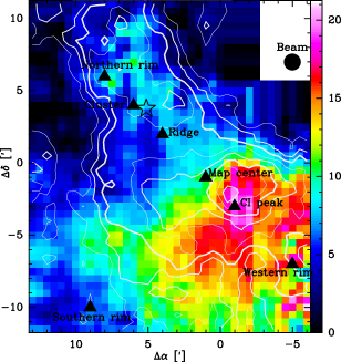
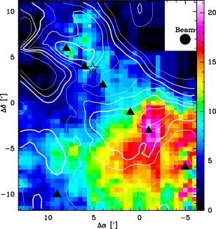
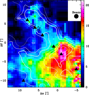
Figure 1: Velocity integrated intensities of [C i] emission (color) overlayed with contours of (a) ¹²CO 4–3, (b) ¹²CO 1–0 and (c) ¹³CO 1–0 integrated intensities at a common angular resolution of 70″. The center of the maps is at $\alpha$ = 03^h44^m10^s, $\delta$ = 32°06′(J2000). All tracers are integrated from V_LSR 2 km s^-1 to 14 km s^-1. Contours range between 20% to 90% with a step of 10% of the peak intensities that are 73 K km s^-1 for ¹²CO 4–3, 72 K km s^-1 for ¹²CO 1–0 and 31 K km s^-1 for ¹³CO 1–0. The seven filled triangles indicates the positions where we carry out a detailed PDR analysis later. The open pentacle symbol denotes the position of HD 281159.

The energy of the upper level for the [C i] 1–0 transition is 24 K and the critical density for this transition is 10³ cm^-3 for collisions with molecular H₂ (Schröder et al., 1991). This implies that [C i] 1–0 is easily excited and the line is easily detectable even when emitted by moderate density interstellar gas exposed to the average interstellar radiation field. Previous observations have found the [C i] to be extended and well correlated with the low-$J$ CO emission (see a review by Preibisch et al., 1996; Schneider et al., 2003; Mookerjea et al., 2006). In IC 348 the [C i] emission peaks to the southwest of the mapped region with a value of 24 K km s^-1 and we detect [C i] emission over a large region with a homogeneous intensity distribution at a level of 65% of the peak intensity. The [C i] emission is extended towards the east and northeast of the mapped region. This is consistent with the clumpy UV irradiated cloud scenario.

The ¹²CO 4–3 emission peaks at almost the same position as [C i] with an intensity of $\sim$ 66 K km s^-1. However, the morphology of the ¹²CO 4–3 emission is different to that of [C i]. We find secondary maxima in the north and a steeper decay of the emission to the south. The distribution of the ¹²CO 4–3 emission agrees very well with that of ¹²CO 3–2 (Sun et al., 2006). We attribute the difference in the intensity distributions of [C i] and ¹²CO 4–3 to the fact that ¹²CO 4–3 emission arises from regions of higher temperature and density, while [C i] emission can arise also from embedded PDR surfaces with moderate to low density within the molecular clouds.

The distribution of the ¹²CO 1–0 emission shows the same global structure as the ¹²CO 4–3 emission, but it is considerably more extended. This is consistent with the fact that ¹²CO 1–0 traces lower temperature and density. The morphologies of [C i] and ¹³CO 1–0 appear to be very similar, implying that they trace the same material and both lines are effectively column density tracers.

We selected seven positions within IC 348 for a more detailed study. Six of the seven positions are oriented along a cut from the northern edge of the cloud, past HD 281159 and into the clouds. The seventh position is at the southeast edge of the cloud. Though emission at the seventh position (southern rim) is weak, it is clearly detected. The selected positions vary in their physical and chemical conditions. Spectra of [C i], ¹²CO 4–3, ¹²CO 1–0 and ¹³CO 1–0 at those seven positions are displayed in Fig. 2.

The [C i] emission is centered at a velocity of $\sim$ 8 km s^-1. The lowest [C i] main beam brightness temperature ($\sim$ 2 K) occurs at the southern rim (9′,-10′), while the highest temperatures of 7.0 K and 6.7 K are observed at the position of the [C i] peak (-1′,-3′) and the western rim (-5′,-7′), respectively. The line widths of [C i] spectra at the seven positions range between 2.0 km s^-1 and 2.6 km s^-1.

The ¹²CO 4–3 main beam brightness temperature varies between $\sim$ 3.6 K at southern rim and 16.4 K at [C i] peak. The line width of the ¹²CO 4–3 spectra ranges between 2.0 km s^-1 and 2.7 km s^-1.

Both the ¹²CO 1–0 and ¹³CO 1–0 spectra consist of two velocity components: one is at $\sim$ 7 km s^-1 and the other lies at $\sim$ 8 km s^-1. The two components are most prominently visible at the southern rim, map center and the [C i] peak. For the 8 km s^-1 component at the [C i] peak, the ¹³CO 1–0 spectrum peaks at the dip of the ¹²CO 1–0 spectrum, which may indicate self-absorption effect for this component.

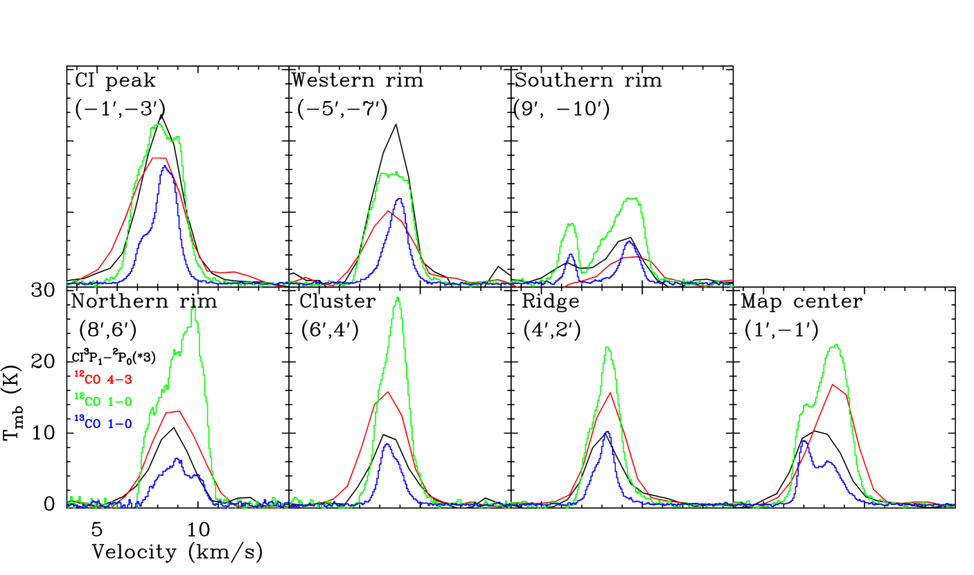
Figure 2: Spectra of the four different tracers on those six positions along the cut from the northern edge of the cloud into the cloud, and on the seventh position at the south of the cloud. [C i] spectra in all the positions have been multiplied by 3. All panels have the same x axis from 3.5 km s^-1 to 14.5 km s^-1 and the same y axis from -0.5 K to 30.5 K.

Table 1 presents the integrated intensities and line ratios at the seven selected positions. Figure 3 shows the variation of the integrated intensities and their ratios at these seven positions.

Table 1: The observed integrated line intensities (in erg s^-1 sr^-1 cm^-2) and line ratios at the seven selected positions. The errors on the integrated intensity are estimated to be $\sim$ 15%.

Position	($\Delta\alpha$,$\Delta\delta$)	[C i]	12CO 4–3	12CO 1–0	13CO 1–0	$\frac{\mathrm{[{C\textsc{i}}]1-0}}{\mathrm{{}^{12}CO4-3}}$	$\frac{\mathrm{[{C\textsc{i}}]1-0}}{\mathrm{{}^{13}CO1-0}}$	$\frac{\mathrm{{}^{12}CO4-3}}{\mathrm{{}^{12}CO1-0}}$
		[10-8 erg s-1 sr-1 cm-2]
Northern rim	( 8′, 6′)	96.56	336.43	9.59	1.74	0.29	55.51	35.07
Cluster	( 6′, 4′)	81.99	365.30	7.14	1.41	0.22	58.01	51.15
Ridge	( 4′, 2′)	75.09	313.20	5.37	1.61	0.24	46.59	58.38
map Center	( 1′,-1′)	106.79	413.27	8.38	2.10	0.26	50.85	49.33
$[{C\textsc{i}}]$ peak	(-1′,-3′)	226.61	548.04	9.31	3.70	0.41	61.23	58.85
Western rim	(-5′,-7′)	172.05	256.15	6.01	2.13	0.67	80.61	42.61
Southern rim	( 9′,-10′)	72.71	60.21	5.50	1.35	1.21	54.02	10.95

In Fig. 3a we see that the intensities of [C i], ¹³CO 1–0 and ¹²CO 4–3 lines show similar trends, only the falling off of the intensity of ¹²CO 4–3 is somewhat less drastic than [C i], ¹³CO 1–0. As opposed to the single peak seen in [C i], ¹³CO 1–0 and ¹²CO 4–3, the ¹²CO 1–0 intensity profile shows two peaks with comparable intensities, one at the northern rim and the other at the position of the [C i] peak.

Three independent line ratios, i.e., [C i] / ¹²CO 4–3, [C i] / ¹³CO 1–0 and ¹²CO 4–3 / ¹²CO 1–0, are presented in Table 1 and Fig. 3b (in erg s^-1 sr^-1 cm^-2). The largest [C i] / ¹²CO 4–3 ratio (1.21) occurs at the southern rim and the second (0.67) and third (0.41) largest are at the western rim and [C i] peak, while the ratios at the other four positions are $\sim$ 0.25. When comparing with other star forming regions like W 3 Main, S 106 and Orion A etc. (see Table 3 by Kramer et al., 2004), the [C i] / ¹²CO 4–3 ratio at the other five positions are within the range found in those star forming regions except for the western and southern rim. The highest ratio at the southern rim is close to the ratio found at the center of M 51 and the nucleus position of NGC 4826 (Israel & Baas, 2002). The ¹²CO 4–3 / ¹²CO 1–0 ratio peaks at [C i] peak and decreases for the positions further away with increasing distance. The [C i] / ¹³CO 1–0 ratios are rather constant except for the western rim.

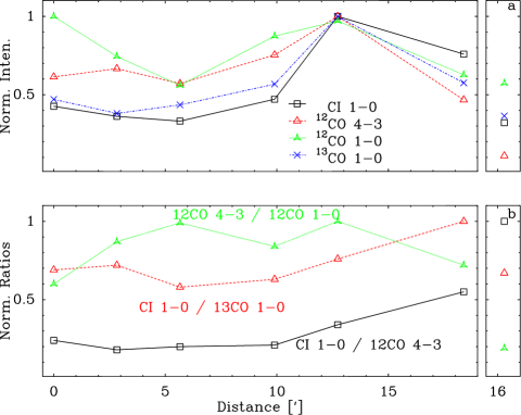
Figure 3: The top panel (a) presents the normalized integrated intensities of [C i], ¹²CO 4–3, ¹²CO 1–0 and ¹³CO 1–0 in the seven selected positions. The typical errors of the intensities are about 15%, resulting in errors of the line ratios of about 21%; (b) displays integrated line intensity ratios. The x axes of all panels are the relative distance to the northern rim (8′,6′) position. The southern rim is plotted in a separate box.

4 LTE Analysis

Figure 4 shows a map of the ¹²CO 4–3 / ¹²CO 1–0 line ratio in terms of line integrated temperatures (K km s^-1) overlaid by ¹²CO 4–3 integrated intensities. The ratio has its minimum of $\sim$ 0.3 at the edges of the cloud; ratios of $\sim$ 0.9 are found at the ¹²CO 4–3 peaks; maximum ratios between 1.1 and 1.5 occur close to HD 281159.

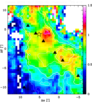
Figure 4: The color plot represents the ¹²CO 4–3 / ¹²CO 1–0 line intensity ratio (in units of K km s^-1) observed in the IC 348 cloud. The contours show the ¹²CO 4–3 line intensity spaced at 10% intervals from 20% to 90% relative to the peak intensity of 73 K km s^-1. White pixels in the figure denote positions where either of the line intensities falls below the 3 $\sigma$ threshold.

For a rough estimate of the column densities and for an easy comparison to other [C i] studies (e.g. Little et al., 1994; Plume et al., 2000; Bensch et al., 2003) we first apply a Local Thermodynamic Equilibrium analysis. Assuming LTE and optically thick emission, the ¹²CO 4–3 / ¹²CO 1–0 ratio of 0.3 corresponds to an excitation temperature $T_{\mathrm{ex}}$ of $\sim$ 10 K. The ratio grows to 0.85 for $T_{\mathrm{ex}}\sim 50$ K and remains almost constant at even higher temperatures. Considering the calibration uncertainty, we set $T_{\mathrm{ex}}$ to 50 K in all the positions where the ratio falls above 0.85. We note that [C i] and ¹²CO often have different excitation temperatures. However, $N$(C)_LTE only changes by 20% when the assumed excitation temperature varies between 20 and 150 K. For the first order estimation, it is therefore reasonable to use the ¹²CO excitation temperature also for [C i]. With the ¹²CO excitation temperatures and the assumption of optically thin [C i] and ¹³CO 1–0 emission, we then obtain the column density of C, $N$(C)_LTE, and ¹³CO, $N$(¹³CO)_LTE, from the integrated line intensities. Using the relative abundance ratio [¹²CO]/[¹³CO] of 65 (Langer et al., 1990) we translate the ¹³CO column densities into CO column densities. H₂ column densities are derived from the [CO]/[H₂] abundance ratio of 8 10^-5 (Frerking et al., 1982). The results are summarized in Table 2.

Table 2: Results of the LTE analysis. The excitation temperature $T_{\mathrm{ex}}$ is listed in Column (2); Column (3) - (5) present C, CO and H₂ column densities; the C/CO ratio is listed in Column (6). The uncertainties of the column densities are derived by varying the integrated intensities by $\pm$15%.

number	$T_{\mathrm{ex}}$	$N$(C)LTE	$N$(CO)LTE	$N$(H2)LTE	C/COLTE
	K	1016[cm-2]	1017[cm-2]	1021[cm-2]
Northern rim	18${}^{47}_{15}$	12.08${}^{19.71}_{9.27}$	9.56${}^{22.84}_{7.16}$	12.50${}^{28.55}_{8.95}$	0.13${}^{0.28}_{0.04}$
Cluster	5020	9.61${}^{11.17}_{7.77}$	16.99${}^{19.54}_{7.33}$	21.24${}^{24.43}_{9.16}$	0.06${}^{0.15}_{0.04}$
Ridge	5028	9.04${}^{10.46}_{7.32}$	19.37${}^{23.03}_{10.43}$	24.21${}^{28.78}_{13.04}$	0.05${}^{0.10}_{0.03}$
Map center	48${}^{50}_{18}$	13.09${}^{16.00}_{10.68}$	24.39${}^{29.03}_{10.25}$	30.49${}^{36.29}_{12.82}$	0.05${}^{0.16}_{0.04}$
$[{C\textsc{i}}]$ peak	5029	26.85${}^{30.88}_{21.71}$	44.47${}^{51.14}_{24.56}$	55.59${}^{63.93}_{30.70}$	0.06${}^{0.13}_{0.04}$
Western rim	28${}^{50}_{15}$	19.72${}^{28.30}_{17.61}$	16.25${}^{29.99}_{9.52}$	20.31${}^{37.49}_{11.90}$	0.12${}^{0.30}_{0.06}$
Southern rim	7${}^{8}_{6}$	37.50${}^{72.57}_{21.96}$	6.66${}^{8.54}_{5.40}$	8.32${}^{10.67}_{6.76}$	0.56${}^{1.34}_{0.26}$

The resulting map of C/CO column density ratios is presented in Fig. 5. In most of the cloud, the C/CO ratio falls below 0.1. Higher values (up to 1.5) occur at the rim of the cloud where the ¹³CO 1–0 emission is more diffuse. Values as low as 0.02 are found at the southwest of the cloud and along the ridge to the northeast. As ¹³CO 1–0 roughly traces the H₂ column density, this plot indicates an anti-correlation between the C/CO ratio and the H₂ column density. This is consistent with the conclusion of Mookerjea et al. (2006) that the [C i] line is not a tracer of optical extinction, total H₂ column density or total mass in the beam.

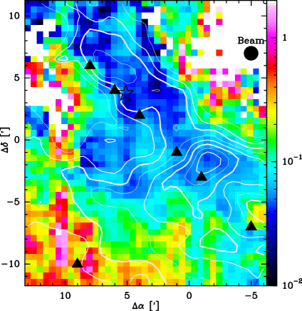
Figure 5: The C/CO column density ratio overlaid by ¹³CO 1–0 integrated intensities contours. The contour levels are spaced at 10% intervals from 20% to 90% relative to the peak intensity of 31 K km s^-1. White pixels in the figure denote positions where the ¹³CO 1–0 intensities fall below the 3 $\sigma$ threshold.

The seven positions, for which we perform a detailed analysis within the context of a PDR model, exhibit C/CO column density ratios between about 0.05 and 0.5, i.e. they cover a relatively wide range (see Table 2). The ratios measured within the full map cover almost the full range cited so far in the literature with values as low as 0.03 in parts of G34.3 (Little et al., 1994) and as high as 1.5 seen in the Polaris Flare (Bensch et al., 2003).

5 PDR Modelling

In the next step we attempt to obtain a self-consistent model for the physical and chemical structure of the cloud matching the observed C/CO ratios. We will use a clumpy PDR model to self-consistently compute the abundance of the species and their excitation determining the line strength. The model is constrained by the strength of the UV field, which can be independently estimated, and by the known geometry, provided by the complex, filamentary, and clumpy structure of the region.

5.1 FUV intensity

5.1.1 Estimate from the FIR continuum

We use HIRES processed 60 and 100 $\mu$m IRAS data (Aumann et al., 1990) to generate a far-infrared intensity map $I_{\mathrm{FIR}}$ in IC 348. It represents the far-infrared intensity between 42.5 $\mu$m and 122.5 $\mu$m as measured by the filter curves of the two IRAS data sets (Nakagawa et al., 1998). Following Kaufman et al. (1999), we assume that the total FUV flux, $\chi_{\mathrm{FIR}}$, absorbed by the dust grains is re-radiated in the far-infrared. In this way we estimate the FUV field from the far-infrared field (cf. Kramer et al., 2005): $\chi_{\mathrm{FIR}}/\chi_{0}=4\pi\leavevmode\nobreak\ I_{\mathrm{FIR}}$, where $\chi_{0}=2.7\times 10^{-3}$ erg s^-1 cm^-2 (Draine, 1978; Draine & Bertoldi, 1996). The derived spatial distribution of the FUV intensity is presented in Fig. 6. In the mapped region, the FUV field $\chi_{\mathrm{FIR}}$ varies between about 1 and 100 Draine units. For the seven selected positions $\chi_{\mathrm{FIR}}$ is listed in Table 3.

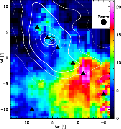
Figure 6: FUV intensity distribution (contours) in IC 348 estimated from the IRAS FIR fluxes, overlayed on the [C i] integrated intensities (colors). The FUV intensity $\chi_{\mathrm{FIR}}$ contour levels run from 5, 10, 20 to 100 by steps of 20 Draine units, $\chi_{0}$.

5.1.2 Estimate from the stellar radiation

The primary source of UV radiation in the cloud is HD 281159. Assuming that the star is a black body at an effective temperature $T_{\mathrm{eff}}$ corresponding to its spectral type, we can estimate the FUV flux independently (Kramer et al., 1996; Beuther et al., 2000). A B 5 V star has an effective temperature $\log(T_{\mathrm{eff}})=4.182$ and a total luminosity $L$ of $\log(L/L_{\odot})=2.681$ (de Jager & Nieuwenhuijzen, 1987). The FUV luminosity $L_{\mathrm{FUV}}$ and the FUV flux $\chi_{\mathrm{FUV}}$ are defined as

$$L_{\mathrm{FUV}}=L\cdot\frac{\Phi_{\mathrm{UV}}}{\Phi_{\mathrm{total}}},\leavevmode\nobreak\ \leavevmode\nobreak\ {\rm{and}}\leavevmode\nobreak\ \leavevmode\nobreak\ \chi_{\mathrm{FUV}}=\frac{L_{\mathrm{FUV}}}{4\pi d^{2}},$$ (1)

where $\Phi_{\mathrm{UV}}$ is the FUV flux between 6 eV and 13.6 eV, $\Phi_{\mathrm{total}}$ is the total flux, and $d$ is the distance to the UV source. We compute the distance $d$ in two ways: for the point close to HD 281159 we use the optical radius of the cluster IC 348 of about 0.37 pc (Herbig, 1998) as the minimum distance between star and cloud. For all other points we assume that star and cloud are located in the same plane so that the distance is directly given by the observed separation. Finally we normalize the FUV field to units of $\chi_{0}$. The resulting FUV fields, $\chi_{\mathrm{star}}$, are also listed in Table 3 for the seven selected positions.

We see that both methods provide consistent FUV field values. Because of the uncertainty of the distance between star and cloud we consider the values $\chi_{\mathrm{FIR}}$, derived from the HIRES data, somewhat more reliable so that we will use them in the following. The FUV field $\chi$ at the seven positions ranges from about 1 to 90 Draine units.

5.2 Clumpy PDR scenarios

Molecular clouds are known for their highly filamentary and clumpy, often self-similar structure over a wide range of scales (Dame et al., 2001; Heyer et al., 1998; Stutzki et al., 1988). The observed structure further breaks up into substructures with every step of increased spatial resolution (Falgarone & Phillips, 1996; Bensch et al., 2001). For IC 348, the self-similar structure was directly measured in terms of the $\Delta$-variance by Sun et al. (2006). In such a cloud, the UV field can penetrate deeply into the cloud forming PDRs at many internal surfaces. The cloud is basically filled by surfaces (Ossenkopf et al., 2007). This explains the observed [C i] and even [C ii] emission deep within molecular clouds (Stutzki et al., 1988; Howe et al., 1991; Stacey et al., 1993; Meixner & Tielens, 1993). We can simulate such a structure by an ensemble of individual clumps, each of them being small compared to the overall cloud, leaving enough “empty” regions to permit a deep penetration of the UV field (Stutzki et al., 1998).

In the following we test two different clump ensembles with respect to their ability to reproduce the observed line intensities.

5.2.1 Modelling of individual clumps

All individual clumps in the PDRs are modelled using the spherical KOSMA - $\tau$ PDR model (Störzer et al., 1996; Röllig et al., 2006, 2007). The model computes the chemical and temperature structure of a clump illuminated by an isotropic FUV radiation field and cosmic rays. The emission from the model is calculated as a function of the gas density, FUV radiation field and mass of the clumps (implicitly specifying the clump size). The model clumps are assumed to have a power-law density profile of $n$(r) $\propto$ $n_{0}$$r^{-1.5}$ for 0.2 $\leq$ $r/r_{\mathrm{cl}}$ $\leq$ 1 and $n$(r) = const. for $r/r_{\mathrm{cl}}$ $\leq$ 0.2. $n_{0}$ is the density at the clump surface called clump density, which is about half of the clump averaged density $\langle n\rangle$: $n_{0}$ $\sim$ $\frac{1}{1.91}$ $\langle n\rangle$.

The PDR models are pre-computed on a regular grid with equidistant logarithmic steps. The FUV field $\chi$ covers the range from $10^{0},10^{0.5},...,10^{5.5},10^{6.0}$ Draine units; The clump densities range from $10^{2.0},10^{2.5},...,10^{5.5},10^{6.0}$ cm^-3; and the clump masses $M_{\mathrm{cl}}$ cover $10^{-3.0},10^{-2.5},...,10^{1.5},10^{2.0}$ M_⊙.

5.2.2 Ensemble of identical clumps (Ensemble 1)

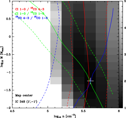
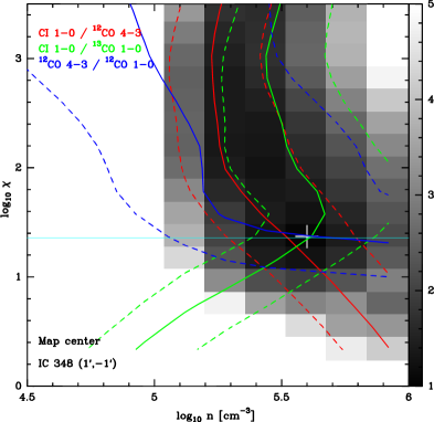
Figure 7: Comparison of the observed line intensity ratios [C i]/¹²CO 4–3, [C i]/¹³CO 1–0 and ¹²CO 4–3/¹²CO 1–0 at (1′, $-1$′) with the single clump KOSMA - $\tau$ PDR model calculations. The left figure shows the fit of clump mass and density at a fixed FUV field $\chi$ of 10^1.5; the right one presents the fit of FUV field and clump density at a fixed clump mass of 10^-1 M_⊙. The central solid contours represent the observed intensity ratios, the outer dashed two give those for a 20% uncertainty. The grey-scale images indicate the reduced $\chi^{2}$ of the fit. The position of the minimum reduced $\chi^{2}$ is marked by a white cross. The horizontal light blue line in the right panel shows the FUV flux $\chi_{\mathrm{FIR}}$ from the HIRES data.

In a first approach we will assume that the cloud is composed of a collection of identical clumps, so that the full ensemble is characterized by the parameter set of the individual clumps and their number only. To determine the properties of the individual clumps we perform a $\chi^{2}$ fit of the three line intensity ratios given in Table 1, using a spherical PDR model in a three-dimensional parameter space spanned by the FUV field, the clump mass, and density. The results for the seven selected positions are summarized in Table 3. Figure 7 presents an example of the $\chi^{2}$ fitting for the map center (1′, $-1$′). The left panel shows a cut through the parameter space for a fixed UV field, demonstrating the fit of clump mass M_cl and clump density $n_{0}$. The right panel presents the corresponding fit for the FUV field $\chi$ and the clump density $n_{0}$. We see that all line ratios are good density tracers, but hardly constrain the clump mass as expected. The clump density has to fall between 2.5 and 5.0 10⁵ cm^-3. But the reduced $\chi^{2}$ only changes between 1 and 2.5 when the clump mass varies from 10^-2.0 to 10^1.0 M_⊙. This general behaviour applies to all positions analyzed. The clump densities at the seven positions vary between 4.4 10⁴ to 4.3 10⁵ cm^-3. The highest clump density occurs at positions of the ridge and the map center. The clump masses are not well constrained, the best fitting values fall between 0.1 and 0.4 M_⊙. The fitted FUV flux $\chi_{\rm PDR}$ agrees with $\chi_{\rm FIR}$ derived from the FIR continuum in most positions. The maximum deviations by a factor three correspond to the maximum deviation that we got comparing the FIR continuum with the stellar radiation estimate.

Table 3: Physical parameters at selected positions in Fig 1, obtained by fitting the observed intensity ratios to the single clump KOSMA - $\tau$ PDR models. Columns (2) - (5) list the fitted clump densities, clump mass, clump radius and FUV field; Column (6) is the minimum reduced $\chi^{2}$ of the PDR fit; the FUV field derived from the FIR continuum $\chi_{\mathrm{FIR}}$ and that from the stellar radiation $\chi_{\mathrm{star}}$ are in Column (7) and (8); The distance to HD 281159 used for the calculation of $\chi_{\mathrm{star}}$is listed in Column (9).

Position	$n$	$M_{\mathrm{cl}}$	Rcl	$\chi_{\mathrm{PDR}}$	$\chi^{2}_{min}$	$\chi_{\mathrm{FIR}}$	$\chi_{\mathrm{star}}$	$d$
	[105cm-3]	M⊙	pc					pc
Northern rim	1.91	0.2	0.01	15	1.38	39	40	0.37
Cluster	2.75	0.1	0.01	98	1.05	84	40	0.37
Ridge	4.25	0.4	0.01	38	1.23	46	40	0.37
Map center	3.98	0.1	0.01	23	1.04	23	13	0.64
$[{C\textsc{i}}]$ peak	1.91	0.1	0.02	23	1.96	11	7	0.90
Western rim	0.63	0.2	0.02	20	2.00	6	3	1.42
Southern rim	0.44	0.4	0.02	2	2.31	1	3	1.29

The total number of clumps in the beam $N_{\mathrm{ens}}$ is calculated by comparing the observed absolute line integrated intensities with the models, correcting for the beam filling factor. A 70″ beam corresponds to a diameter of 0.10 pc at the distance of IC 348. The clump size obtained from the best fit models found in the previous section ranges from 0.01 to 0.02 pc. The beam filling factor $\eta_{\mathrm{bf,i}}$ of each clump is calculated as $\eta_{\mathrm{bf,i}}=\Omega_{\mathrm{cl}}/\Omega_{\mathrm{beam}}$, where $\Omega_{\mathrm{cl}}$ and $\Omega_{\mathrm{beam}}$ are the solid angles of a clump and the beam. $\Omega_{\mathrm{cl}}=\pi R_{\mathrm{cl}}^{2}/D^{2}$ is the solid angle of the individual clump. $D$ is the distance of the cloud; assuming a Gaussian beam shape, $\Omega_{\mathrm{beam}}$ is computed as $\Omega_{\mathrm{beam}}=\pi\theta_{\mathrm{beam}}^{2}/4\ln 2$, where $\theta_{\mathrm{beam}}$ is the FWHM of our beam. The intensity correction for a single clump is $I^{\mathrm{\prime}}_{\mathrm{i}}=I_{\mathrm{mb,i}}/\eta_{\mathrm{bf,i}}$, where $I_{\mathrm{mb,i}}$ is the beam averaged line intensity for that single clump. Since [C i] is the most optically thin one among our four tracers, we use its line intensity to derive the number of clumps in the beam $N_{\mathrm{ens}}$ (see Table 4) by dividing the observed intensities $I_{\mathrm{[{C\textsc{i}}]obs}}$ by the intensities for a single clump $I_{\mathrm{[{C\textsc{i}}]mod,i}}$

$$N_{\mathrm{ens}}=\frac{I_{\mathrm{[{C\textsc{i}}]obs}}}{I_{\mathrm{[{C\textsc{i}}]mod,i}}\cdot\eta_{\mathrm{bf,i}}}=\frac{I_{\mathrm{[{C\textsc{i}}]obs}}}{I_{\mathrm{[{C\textsc{i}}]mod,i}}}\times\frac{\Omega_{\mathrm{beam}}}{\Omega_{\mathrm{cl}}}.$$ (2)

Table 4: Results of ensemble of identical clumps, Ensemble case 1. The mass and FUV field for each single clump are listed in Column (2) and (3); Column (4) - (6) present the line intensity ratios between the ensemble models and observations of ¹²CO 4–3, ¹²CO 1–0 and ¹³CO 1–0; The C, CO and H₂ column densities from the ensembles are presented in Column (7), (8) and (9); Column (10) is the C/CO ratios. The total number of the clumps in the ensemble and ensemble mass are listed in Column (11) and (12); Column (13) lists the beam filling factor of each clump. The total ensemble mass $M_{\mathrm{ens}}$ listed in the table is computed as $M_{\mathrm{ens}}=N_{\mathrm{ens}}\times M_{\mathrm{cl}}$, where $M_{\mathrm{cl}}$ is the mass of a clump.

Position	$M_{\mathrm{cl}}$	$\chi_{\mathrm{en1}}$	$R_{\mathrm{{}^{12}CO4-3}}$	$R_{\mathrm{{}^{12}CO1-0}}$	$R_{\mathrm{{}^{13}CO1-0}}$	$N$(C)ens	$N$(CO)ens	$N$(H2)ens	C/COens	$N_{\mathrm{ens}}$	$M_{\mathrm{ens}}$	$\eta_{\mathrm{bf,i}}$
	M⊙					1016[cm-2]	1017[cm-2]	1021[cm-2]			M⊙
Northern rim	0.32	10	0.63	0.67	0.87	13.97	18.58	7.72	0.075	4.59	1.47	0.17
Cluster	0.10	100	1.07	0.99	1.13	10.02	21.56	8.90	0.046	16.75	1.68	0.04
Ridge	0.32	32	0.95	1.13	0.95	8.90	29.49	11.29	0.030	6.72	2.15	0.08
Map center	0.10	32	0.94	1.05	0.97	13.25	34.24	13.05	0.039	24.56	2.46	0.04
$[{C\textsc{i}}]$ peak	0.10	32	0.94	1.59	0.83	31.54	29.88	13.14	0.106	24.74	2.47	0.08
Western rim	0.10	10	0.78	1.43	0.71	24.52	9.33	6.10	0.263	11.51	1.15	0.17
Southern rim	0.32	1	0.84	0.81	0.74	14.62	6.28	3.03	0.233	5.70	1.82	0.17

Then we use $N_{\mathrm{ens}}$ to calculate the ratios $R$ of line intensities between model ensemble and observations for the other tracers:

$$R=\frac{N_{\mathrm{ens}}\cdot I_{\mathrm{mod,i}}\cdot\eta_{\mathrm{bf,i}}}{I_{\mathrm{obs}}}.$$ (3)

The $R$ values are listed in Table 4. This allows easy judgment of the quality of the model fit. Considering the calibration uncertainty, a perfectly fitting model yields a ratio $R$ of 1$\pm$0.15. All three remaining tracers from Ensemble 1 have a good agreement between the modelled and observed absolute line intensities.

5.2.3 Clumps with a mass and size spectrum (Ensemble 2)

Representing the clumpy structure of the cloud by an ensemble of identical clumps is, of course, an oversimplification. A realistic clump size and mass distribution should be taken into account. Large-scale CO maps present the clumpy structure of the ISM with a mass distribution following a power law $dN/dM\propto M^{\mathrm{-\alpha}}$, where $N$ is the number of clumps and $\alpha$ has a value around 1.8 (Kramer et al., 1998b). Furthermore, the observations also show that there is a strong correlation of the density and mass of the clumps corresponding a mass-size relation $r\propto M^{\mathrm{\gamma}}$ with $\gamma\approx$ 2.3 (Heithausen et al., 1998). For an ensemble of randomly positioned clumps with a power law mass spectrum, there is a relation among the power law spectral index $\beta$ of the power spectrum, $\alpha$ and $\gamma$: $\beta=\gamma(3-\alpha)$ (Stutzki et al., 1998). Using the $\alpha$ and $\gamma$ values above, $\beta=2.76$, which is close to the power law index $\beta=2.71$ of ¹³CO 2–1 in IC 348 found by Sun et al. (2006).

In this Section we assume these characteristics to be universal and model the emission by ensemble averaging the PDR single clump results over such a clump distribution (Cubick, 2005; Cubick et al., 2008) to reproduce the observed line intensities. The remaining parameter space is then given by the FUV field input $\chi_{\rm ens}$, the total mass within the beam $M_{\mathrm{ens}}$, the average clump ensemble density $n_{\mathrm{mean}}$, and the minimum and maximum clump masses, $m_{\mathrm{cl}}^{\mathrm{min}}$ and $m_{\mathrm{cl}}^{\mathrm{max}}$.

To constrain the fit to a three-dimensional parameter space also for this case, we fix the clump mass limits. The upper mass limit has to reflect the total mass of the clump distribution because a spectral index $\alpha=1.8$ corresponds to a top-heavy function, i.e. a distribution where most of the mass is contained in the few most massive clumps. We assume that the total mass obtained from the Ensemble 1 model also provides a reasonable guess for the total mass in Ensemble 2, consequently setting the upper mass limit $m_{\mathrm{cl}}^{\mathrm{max}}$ to half of the total mass of Ensemble 1. We set the lower mass limit, $m_{\mathrm{cl}}^{\mathrm{min}}$, to 10^-2 M_⊙. These small clumps can only exist transiently and evaporate on a time scale of $\sim$ 5000 yrs (Kramer et al., 2008). The choice of the lower mass limit is not critical for the fit. Cubick et al. (2008) studied the dependencies of the model output on the clump mass limits and found that mainly high - $J$ CO transitions (like ¹²CO 8–7) are sensitive to the lower clump mass limit.

Table 5: Results of ensembles with a clump mass distribution and mass-size distribution, Ensemble case 2. Column (2) - (4) present the ratios (in erg s^-1 sr^-1 cm^-2) of the modelled and observed line intensities for ¹²CO 4–3, ¹²CO 1–0 and ¹³CO 1–0; The mean clump ensemble density $n_{\mathrm{mean}}$ and the fitted FUV field $\chi_{\mathrm{en2}}$ are presented in Column (5) and (6). The C, CO and H₂ column densities from the ensembles are presented in Column (7), (8) and (9); Column (10) is the C/CO ratios. The total masses are listed in Column (11); Column (12) is the minimum reduced $\chi^{2}$ of the fit.

Position	$R_{\mathrm{{}^{12}CO4-3}}$	$R_{\mathrm{{}^{12}CO1-0}}$	$R_{\mathrm{{}^{13}CO1-0}}$	$n_{\mathrm{mean}}$	$\chi_{\mathrm{en2}}$	$N$(C)ens	$N$(CO)ens	$N$(H2)ens	C/COens	$M_{\mathrm{ens}}$	$\chi^{2}_{min}$
				[105cm-3]		1016[cm-2]	1017[cm-2]	1021[cm-2]		M⊙
Northern rim	1.00	1.04	1.44	3.2	3	14.36	51.82	19.28	0.028	3.84	1.43
Cluster	1.06	1.03	1.13	3.2	100	9.88	25.58	9.93	0.039	1.97	0.23
Ridge	1.13	1.26	0.91	3.2	32	9.05	23.43	9.10	0.039	1.83	0.50
Map center	1.08	1.19	1.08	3.2	10	13.78	40.71	15.39	0.034	3.07	0.29
$[{C\textsc{i}}]$ peak	1.13	1.73	0.86	1.0	10	31.24	40.16	16.61	0.078	2.88	2.37
Western rim	1.83	2.03	1.13	1.0	10	30.49	23.72	12.61	0.078	2.19	3.37
Southern rim	1.06	0.84	0.66	0.3	1	13.58	5.24	2.62	0.259	0.53	4.91

The actual fit is performed analogously to the ensemble 1 case. The results are presented in Table 5. We find a reasonable agreement between the modelled line intensities from Ensemble 2 and the observed ones. The intensity ratios between model and observations range between 0.7 and 2.0. The fitted FUV field $\chi_{\mathrm{en2}}$ from Ensemble 2 is consistent with the field $\chi_{\rm ens}$ from Ensemble 1 and that derived from the FIR continuum in most positions. The maximum deviation occurs at the northern rim.

The reduced $\chi^{2}$ values are similar for both ensembles at values less than 5. In spite of the somewhat more complex model, the fit is not better than for an ensemble of identical clumps (Ensemble 1).

To compare the observed absolute line intensities with the model prediction, we show two examples of observed and modelled integrated intensities versus frequency, namely the cooling curves of ¹²CO, ¹³CO (upto $J$ = 9–8) and [C i] for the best-fit of both Ensemble 1 and Ensemble 2 models at the northern rim and the southern rim (see Fig. 8). At those two positions the modelled and observed line intensities agree very well. Fig. 8 also provides a prediction for line intensities of [C i] ³P₂ – ³P₁, ¹²CO 7–6, ¹³CO 8–7, etc. Fig. 8 indicates that the tracers studied in this paper do not allow to draw any conclusion about the clump size spectrum that best fits the observations. Both Ensemble 1 and 2 fit the observed data equally well. On the other hand, they give very different predictions for the higher $J$ CO lines. The line intensities predicted for Ensemble 2 are noticeably larger than those predicted for Ensemble 1 (see Fig. 8). The ¹³CO 8–7 line, tracing the column densities of the warm gas, is predicted to be very sensitive to the differences between the two models, allowing to discriminate between them.

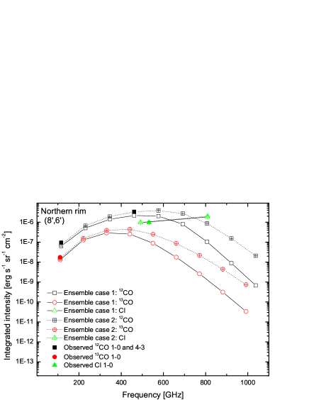
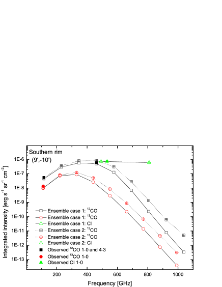
Figure 8: Observed (filled symbols) and modelled line intensities of ¹²CO, ¹³CO, and [C i] from both Ensemble case 1 (drawn lines with open symbols) and Ensemble case 2 (dotted lines, open symbols with a cross inside) at the northern rim (left panel) and the southern rim (right panel). To better display the data, we artificially shift the [C i] frequency by +40 GHz for the observed intensity.

Based on the CO and H₂ column densities from the PDR analysis, we find the averaged CO relative abundance [CO]/[H₂] is $\sim$ 2.4 10^-4, which is 3 times larger than the canonical ratio [CO]/[H₂] of 8 10^-5 (Frerking et al., 1982) that we used in the LTE analysis. The beam averaged C/CO abundance ratio (Table 5) varies by a factor 10 between 0.03 at the northern rim, which shows the highest column density of all studied positions of $2\,10^{21}$ cm^-2, and 0.26 at the southern rim, which shows the lowest H₂ column density of $3\,10^{21}$ cm^-2. The observed anti-correlation between C/CO and N(H₂) and also the absolute values resemble those found in many other Galactic molecular clouds as compiled recently by Mookerjea et al. (2006). They used the KOSMA-$\tau$ model to interpret data taken in the Cepheus B star forming region. They suggested that the emission of high column density peaks is dominated by massive clumps exhibiting low C/CO ratios, while positions of low column densities are dominated by smaller clumps, exhibiting higher C/CO ratios. This scenario is confirmed in IC 348 by a more complete analysis using clump mass ensembles following the canonical mass and size distributions. However, the scatter of the present data is large. Observations of the higher lying transitions of [C i] and CO are needed to further improve the analysis.

6 Summary and Conclusions

We have presented fully sampled [C i] and ¹²CO 4–3 maps of the IC 348 molecular cloud, covering a region of 20′$\times$ 20′. The observed ¹²CO 4–3/¹²CO 1–0 ratios vary between 0.2 and 1.5. High ¹²CO 4–3/¹²CO 1–0 ratios occur near the B 5 star, at the cloud center and northern edge of the cloud.

We have estimated the FUV field from the FIR continuum intensities obtained from the 60 and 100 $\mu$m HIRES/IRAS images. The FUV field in the whole observed region ranges between 1 and 100 Draine units. We also used HD 281159, the primary source of UV radiation in this region, to estimate the FUV field for the seven studied regions and the FUV field varies between 3 to 40 Draine units.

Using a clumpy PDR model based on the spherical KOSMA - $\tau$ PDR model we fitted the observed line intensities and intensity ratios at seven selected positions. The observed intensity ratios provide a strong constraint on the clump densities. They fall between 4.4 10⁴ cm^-3 and 4.3 10⁵ cm^-3. The FUV field fitted in the model falls between 2 to 100 Draine units, consistent with independent estimates for the FUV field derived from the FIR continuum maps by IRAS and from the stellar radiation. We found that both an ensemble of identical clumps (Ensemble 1) and a model using a clump size and mass distribution following the typically observed scaling (Ensemble 2) produce line intensities which are in good agreement (within a factor $\sim 2$) with the observed intensities. The models confirm the anti-correlation between C/CO abundance ratio and hydrogen column density found in many regions and explained by Mookerjea et al. (2006).

The results of this study strengthen the picture of molecular clouds as highly fragmented, surface dominated objects. Although Ensemble 2 is the natural case in this picture, Ensemble 1 fits the observed intensities equally well. We predicted line intensities for [C i], CO, and ¹³CO transitions for both cases, which can be tested by future observations. The higher $J$ CO lines are needed to decide on the necessity of the clump mass and size distributions and to determine the clump mass limits (Cubick et al., 2008).