The FRII Broad Line Seyfert 1 Galaxy: PKSJ 1037-2705

Abstract

In this article, we demonstrate that PKSJ 1037-2705 has a weak accretion flow luminosity, well below the Seyfert1/QSO dividing line, weak broad emission lines (BELs) and moderately powerful FRII extended radio emission. It is one of the few documented examples of a broad-line object in which the time averaged jet kinetic luminosity, $\overline{Q}$, is larger than the total thermal luminosity (IR to X-ray) of the accretion flow, $L_{bol}$. The blazar nucleus dominates the optical and near ultraviolet emission and is a strong source of hard X-rays. The strong blazar emission indicates that the relativistic radio jet is presently active. The implication is that even weakly accreting AGN can create powerful jets. Kinetically dominated ($\overline{Q}>L_{bol}$) broad-line objects provide important constraints on the relationship between the accretion flow and the jet production mechanism.

1 Introduction

It is unclear how the enormous stored energy in the radio lobes of powerful FRII radio sources is related to the thermal luminosity of the accreting gas that flows toward the central black hole. On the one hand, it seems reasonable to expect them to be unrelated, since the bulk of the lobe plasma was ejected from the central engine $\sim 10^{7}$ years earlier than the optical flux from the accretion flow. Therefore, one expects to find many or most FRII sources with fossil lobes, no jets and a weak accretion flow. Yet surprisingly, low frequency surveys such as the 3C survey (which are biased towards sources with strong lobes, i.e. steep spectrum radio emission) contain many sources with FR II lobes in which high dynamic range observations reveal jets that can be traced back to the central quasar, within the resolution of the radio telescope ($\sim$ 1kpc for nearby sources) and many others have strong radio cores and jets on VLBI (parsec) scales (eg, Cygnus A, 3C 175, 3C 334, 3C 215) (Bridle et al, 1994; Punsly, 2001). On the other hand, there has been considerable research attempting to connect the accretion state with the jet kinetic luminosity, $Q$ - with the conflicting conclusions being the subject of much controversy (Rawlings and Saunders, 1991; Willott et al., 1999; Wang et al., 2004; Boroson, 2002). A truly rigorous and unbiased analysis of the connection between the accretion state and $Q$ cannot exclude all of the optically weak FRII radio sources a priori, the narrow line radio galaxies (NLRGs). Many or all of the NLRGs are optically obscured by dusty molecular gas, so a proper treatment must probe inside this gas by looking at the Mid-IR emission. Alternatively, some NLRGs might have weak central AGN and are not significantly obscured. The Spitzer Telescope Mid-IR analysis of a large sample of nearby 3C FRII NLRGs in Ogle et al (2006) seemed to indicate that there was a roughly equal mix of FRII NLRGs that had no hidden quasar and those that had a hidden quasar. The implication is that there is a weak central AGN in many of the FRII objects, of which a large proportion have unobstructed lines of sight to the accretion disk. Conversely, Cleary et al 2007 analyzed an even larger sample of Spitzer observations of 3C FRII sources (NLRGS and QSOs) and concluded that orientation effects alone accounted for the differences in FRII NLRGs and FRII QSOs - i.e., for the most part NLRG had hidden QSOs of the same strength as in FRII QSOs.

Another closely related debate in the literature is the relationship of accretion luminosity, $L_{bol}$ (which is sometimes expressed in a related form in terms of the Eddington ratio, $R_{Edd}=L_{bol}/L_{Edd}$; where $L_{bol}$ is the bolometric thermal luminosity of the accretion flow and $L_{Edd}$ is the Eddington luminosity) to the jet kinetic luminosity, $Q$. For example, Boroson (2002) concluded that a small $R_{Edd}$ is conducive to strong jets in quasars. The study in Wang et al. (2004) was an attempt to correlate various properties of the accretion flow with the jet power. They concluded that $Q/L_{bol}$ and $L_{bol}/L_{Edd}$ were inversely correlated in blazars. The inverse correlation claimed between $Q/L_{bol}$ and $L_{bol}/L_{Edd}$ in Wang et al. (2004), although true, is a trivial consequence of the fact that $Q$ is very weakly correlated with $L_{bol}$ in quasars (the subpopulation of blazars in their sample that excluded BL-Lacs) and not unexpectedly, $L_{bol}/L_{Edd}$ and $L_{bol}$ are strongly correlated in quasars (Punsly and Tingay, 2005). Thus, it was straightforward by means of a partial correlation analysis to demonstrate that inverse correlation between $Q/L_{bol}$ and $L_{bol}/L_{Edd}$ is a spurious correlation (Punsly and Tingay, 2005).

Clearly, powerful extragalactic jets occur in high accretion thermal luminosity systems, the FRII quasars. In fact, some powerful FRII quasars have $L_{bol}>10^{47}\mathrm{ergs/sec}$ (Punsly and Tingay, 2005). The fundamental question is whether low luminosity accretion flows can also power FRII jets. The answer to this question will constrain the dynamics of plausible central engines that can power FRII jets. In order to shed more light on these matters, we have actively searched for FRII radio sources with direct, unambiguous observational evidence of a low luminosity accretion flow below the Seyfert 1/QSO dividing line: a total thermal luminosity (IR to X-ray) of the accretion flow, $L_{bol}<2\times 10^{45}\mathrm{ergs/s}$ (which is shown in section 3.2 to be equivalent to the conventional dividing line between Seyfert 1 and QSO broad-line objects, $M_{V}=-23$). To accomplish this, one requires strong evidence for a direct line of sight to the nucleus as in a nearly pole-on view, such as a blazar line of sight. Secondly, it is preferable to have two metrics of $L_{bol}$, since the optical/UV continuum is often highly contaminated by the high frequency synchrotron tail of the jet emission and is at best an upper bound to the optical/UV flux from the accretion flow. The line strength of one or more broad UV emission lines is a more direct way to measure the accretion flow luminosity in blazars. Previously, we reported on the most extreme blazar in this family, 3C 216 with $L_{bol}\gtrsim 10^{44}\mathrm{ergs/s}$ and a long term time averaged jet kinetic luminosity, $\overline{Q}>10^{46}\mathrm{ergs/s}$, (Punsly, 2006). In fact it was shown that $\overline{Q}>L_{Edd}$ in 3C 216.

This article describes the broadband properties of the core dominated radio source PKSJ 1037-2705. It was previously identified as a broadline AGN at z=0.567 from an optical spectrum with uncalibrated flux (Gutierrez, 2006). The radio observations presented in section 2 of this paper, indicate lobe emission with a 5 GHz luminosity typical of an FRII radio source. The implication is that the time averaged jet kinetic luminosity, $\overline{Q}\sim 5.0\times 10^{44}\mathrm{ergs/s}$ (In this paper we assume: $H_{0}$=70 km/s/Mpc, $\Omega_{\Lambda}=0.7$ and $\Omega_{m}=0.3$). In section 3, new calibrated optical observations are presented that indicate a broad MgII emission line ($\sim 4000$ km/s), and the line strength is consistent with a radio source that has a very low accretion flow thermal luminosity, $L_{bol}\gtrsim 10^{44}\mathrm{ergs/s}$ (well below the Seyfert 1/QSO dividing line). If it were not for the powerful jet seen in a pole-on orientation, PKSJ 1037-2705 would be a very ordinary Seyfert 1 galaxy: $L_{bol}\gtrsim 10^{44}\mathrm{ergs/s}$.

2 Radio Observations

The Australia Telescope Compact Array (ATCA) was used to obtain observations of PKSJ 1037-2705 on November 28, 2002. The source was simultaneously observed at frequencies of 4.8 and 8.64 GHz for 12 hours in the 6A array configuration. The bandwidth was 128 MHz at both frequencies, dual polarization. The radio maps at 4.8 GHz and 8.64 GHz are shown in figure 1.

Figure 1: ATCA radio maps at 4800 and 8640 MHz, from left to right. At 4800 MHz, the beam-size is 1.75”$\times$ 3.55” at a position angle of $-1.5^{\circ}$. Contour levels for the Stokes I emission are 1.26 mJy/beam $\times$ (-0.00125, 0.00125, 0.0025, 0.005, 0.01, 0.02, 0.04, 0.08, 0.16, 0.32, 0.64). The peak fractional polarization is 26.3%. The vector lengths represent 5.7% fractional polarization per arcsecond. At 8640 MHz, the beam-size is 1.03”$\times$ 1.92” at a position angle of $-1.5^{\circ}$. Contour levels for the Stokes I emission are 1.07 mJy/beam $\times$ (-0.005, 0.005, 0.01, 0.02, 0.04, 0.08, 0.16, 0.32, 0.64). The peak fractional polarization is 23.9%. The vector lengths represent 8.2% fractional polarization per arcsecond.

The components were segregated as an unresolved core, an eastern jet and a northern diffuse region. The core flux density distribution was modeled as a single Gaussian component. The jet and the northern component flux densities were integrated by hand: i.e., the residual flux density after subtracting off the Gaussian core from the image was summed to the east (identified as the jet) and to the north. The component fluxes in the 4800 MHz image are: core flux density = $136.1\pm 13.6$ mJy, jet flux density = $25.7\pm 2.6$ mJy and the northern diffuse flux density = $8.2\pm 0.9$ mJy. At 8640 MHz, the component fluxes are: core flux density = $116.3\pm 11.6$ mJy and a jet flux density = $13.8\pm 1.4$ mJy. The error is given by the $10\%$ absolute flux calibration error added in quadrature to the rms noise. Modeling the jet flux density distribution as a single Gaussian gave a similar result. Similarly, summing the cleaned components in the u-v plane reproduced the hand integrations in the northern diffuse region and the jet to within a few percent. The northern diffuse emission was not detected at 8.64 GHz. The northern diffuse flux density in the 8.64 GHz map is $<1.7$ mJy (the 3$\sigma$ rms noise). Defining the radio spectral index, $\alpha$, as $F_{\nu}\propto\nu^{-\alpha}$, we find that the core is flat spectrum $\alpha=0.3$. The jet is extremely steep spectrum, for a jet, $\alpha=1.1$, over 90% of radio jets have $0.5<\alpha<0.9$ (Bridle and Perley, 1984). Furthermore, the northern diffuse component is unrealistically steep, $\alpha>2.5$. Clearly, significant amounts of optically thin flux is missing due to a lack of short interferometer spacings at 8.64 GHz (and possibly at 4.8 GHz as well). Therefore, the jet and diffuse component spectral indices are subject to some systematic uncertainties that we cannot easily quantify. The complete absence of diffuse flux at 8.64 GHz to the north in a relatively small (for a lobe) region, $\sim$ 5 arcsec across, makes it likely that the northern component is very steep spectrum, regardless of any systematic uncertainties. Strictly, speaking, the eastern jet and northern diffuse component flux density should be considered as lower limits, even at 4.8 GHz.

2.1 A Component Model of the Radio Emission

In order to assess the amount of diffuse flux that was missed by the sparse array spacings, we consider the low frequency part of the radio spectrum from archival TXS survey data.

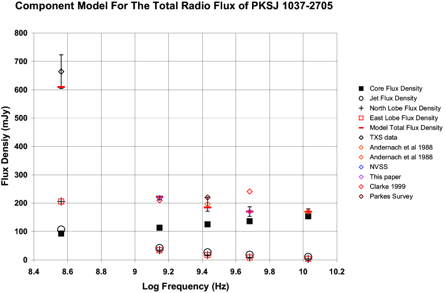
Figure 2: A component model for the broadband radio spectrum of PKSJ 1037-2705. The radio data is drawn from our observations, the NASA Extragalactic Database and archival literature. If the error bars are smaller than the size of the marker for the observation then they are not indicated in the figure. The model consists of a flat spectrum radio core ($\alpha=-0.15$), a kpc scale jet ($\alpha=0.70$) and a pair of steep spectrum lobes ($\alpha=1.25$) with equal flux densities (assumed bilateral symmetry, to first order). The steep lobe spectrum seems to be required by the 1.4 GHz data combined with the 365 MHz data

Figure 2 is a component model that was created to explain the broadband radio data. Before going into the details of the model, the salient point is that there is a huge excess of low frequency emission that cannot be explained without a significant steep spectrum component. The figure contains all known archival data points except the PMNJ survey point which was deleted for the sake of visual clarity, but is discussed below. The need to produce a detailed model of the components is rather apparent from the results of a direct extrapolation of the 4.8 GHz data to lower frequency. Using the two point spectral indices (from 4.8 GHz to 8.64 GHz) and the component fluxes, one predicts a 1.4 GHz flux density for PKSJ 1037-2705 that is over 100% larger than is observed in (see figure 2). A more sophisticated analysis is in order.

2.1.1 The Unresolved Radio Core

First of all, the archival data clearly indicates a variable core. We note that our previous 4.8 GHz VLA, C-Array (relatively low resolution) data in Clarke (1999) indicated a total flux density of 241 mJy about 40% larger than that inferred from our ATCA observation ($170\pm 17$ mJy) and the archival PMNJ data ($175\pm 14$ mJy) in NED. Such large radio variability is characteristic of blazars. Since the radio data is not simultaneous, any model of the core will be inaccurate subject to the scatter associated with the blazar variability. Clearly, the simultaneous (to the 5 GHz) 1.4 GHz C-Array VLA data form Clarke (1999) of 210 mJy shows that the core had an inverted spectrum (contrary to our present measurement) at that time. The relatively large flux density at 10.7 GHz relative to 2.7 GHz flux density found by Andernach et al (1988), considered in conjunction with the steep spectrum lobe and jet components, strongly suggests that the core spectrum was inverted at that epoch as well. Thus, for the model to be an ”average” representation over time, we chose a slightly inverted spectrum, $\alpha=-0.15$ and a flux density of 136 mJy as we measured with ATCA.

2.1.2 The Eastern Jet/Lobe Emission

Any reasonable choice of jet model will not affect our conclusion that the 365 MHz data is only explained by a predominantly steep spectrum component that is modest or small at higher frequencies. It is curious that the jet emission is is extremely steep spectrum. A jet spectral index above 1.0 is extremely rare (Bridle and Perley, 1984). The 4.8 GHz map in Figure 1 reveals some excess diffuse emission to the north of the jet axis. Thus it is likely best to think of the eastern jet as the eastern jet/lobe emission. A significant amount of diffuse steep spectrum flux that is co-spatially projected onto the sky plane with the jet would help to explain the anomalously steep spectrum of the putative eastern jet. Besides the steep spectral index, there is other evidence that a portion of the eastern emission is from a lobe seen along the jet axis, namely the peak of the polarization in figure 1 is not at the end of the ”linear” feature (the terminus of the linear feature is $\approx 85-90$ kpc east of the core: there are 7.8 kpc/arsec at this redshift for our adopted cosmology) as would be expected if the jet terminated in a hot-spot (Bridle et al, 1994; Barthel et al, 1990). To the contrary, there is virtually no detected polarized flux at the end of the linear feature. Instead a highly polarized region is located within $\approx 55$ kpc east of the core. The magnetic field is orthogonal to the jet direction as is indicative of a strong knot in an FRII jet or a terminating hot-spot coincident with the total intensity peak, $\approx 55-60$ kpc to the east of the core (Bridle et al, 1994; Barthel et al, 1990). Thus, the radio map is consistent with a hot spot $\approx 55-60$ kpc from the core that terminates a pole-on jet. The lobe might also be seen pole-on. In this interpretation, the projection of the lobe (that is fed by the eastern jet) onto to the sky plane in the 4.8 GHz map is a diffuse circular patch $\approx 55$ kpc in diameter that is centered $\approx 55-60$ kpc slightly north of due east from of the core. The data is consistent with this interpretation, but not definitive. In any eventuality, the true jet flux is the total eastern flux minus the eastern lobe flux (which we will discuss below). Approximately 40% of kpc scale jets have spectral indices between 0.6 and 0.7. Thus, for the residual jet emission we picked a spectral index of 0.7 in the composite model in figure 2. Again, any reasonable choice of jet model will not affect our conclusion that the 365 MHz data is only explained by a predominantly steep spectrum component that is modest or small at higher frequencies.

2.1.3 Lobe Emission

PKSJ 1037-2705 is likely a standard core dominated radio source that is being viewed pole-on making the de-projection of components complicated. The variable, flat-spectrum core typically represents a jet beamed toward earth and the eastern kpc-scale jet might also be beamed towards earth. The TXS 365 MHz observation constrains the lobe flux and can be used in conjunction with the high frequency radio maps to construct a model of the lobe emission. The radio maps are produced from sparse array spacings so we have likely missed extended flux at 4.8 GHz and almost certainly at 8.64 GHz. Considering this circumstance in conjunction with our inability to extricate lobe flux superimposed on the jet (or co-spatial in sky plane projection with the core), the 8.2 mJy is clearly a lower bound on the extended flux density at 4.8 GHz.

At a minimum, there is $8.2$ mJy of diffuse flux (to the north of the core) in the 4.8 GHz map. The map seems to indicate a diffuse lobe $\approx 55$ kpc in diameter. Based on the morphology of blazars, it is not unusual for the lobe emission on the counter-jet side to appear displaced on the sky plane roughly orthogonal to the jet axis (Antonucci and Ulvestad, 1985). We emphasize that there is likely more lobe flux than this that is either hard to extricate from the brighter features or was possibly missed due to the sparse array spacings. If the source has bilateral symmetry, 16.4 mJy = $2\times 8.2$ mJy might be a more appropriate estimate for the lobe flux density (half from the near lobe and half from the far lobe). The near lobe on the jet side is not readily discernible, perhaps its projection onto the sky plane could be confused with the powerful core or with the bright eastern jet. A co-spatial projection onto the sky plane of an extremely steep diffuse lobe would explain the incredibly steep jet spectrum.

It is interesting to compare this conservative estimate of 16.4 mJy of 4.8 GHz extended emission with the TXS data point in figure 2. The absence of an extended flux detection at 8.64 GHz to the north of the radio core strongly suggests that this is very steep spectrum lobe emission. The sources in the 3C catalog that have steep spectrum lobes, typically have $\alpha\gtrsim 1$ between 750 MHz and 5 GHz (Kellermann et al, 1969). Using 3C radio sources as a guide, we don’t expect the spectral index from 5 GHz to 151 MHz to be any steeper than 1.25 (see the 3C 368 data in NED). The same range ($1<\alpha<1.25$) seems to hold with the steep spectrum 7C catalog sources (Willott et al., 1999). Thus, we pick $\alpha=1.25$ for the PKSJ 1037-2705 lobe emission with 16.4 mJy at 4.8 GHz. After these assignment of component flux densities and spectral indices, the fit to the broad band data in figure 2 is reasonable considering the variable core flux density and the large error in the TXS data. There is no other way to explain the TXS data and the 1.4 GHz data in figure 2 without a steep spectrum lobe component.

2.2 Estimating The Jet Kinetic Luminosity

Ostensibly, one can use the jet emission from the parsec scale radio core to estimate, $Q$ at an epoch of emission that is within a few years of the epoch of accretion flow emission as in Celotti et al (1997). Considering the potential variability in radio loud AGN (which could be large if the epochs are well separated in time, especially in blazars), simultaneous observations in all bands would be ideal for most accurate assessment of the relation between $L_{bol}$ and $Q$. Unfortunately, such estimates are prone to be very inaccurate. One is observing a very small amount of dissipated energy such as X-ray or optical emission as the powerful radio jet propagates away from the source. One must then try to figure out the small fraction of $Q$ that is dissipated in this region. Typically, the X-ray, radio and optical regions are observed with different spatial resolution, so it is unclear if one is detecting the same physical region on parsec scales as one synthesizes the broad band data. In cases in which there is sufficient broad band flux to make an estimate, one is plagued with the further ambiguity of determining the Doppler factor of the relativistic jet. This is a critical obstacle because the luminosity from an unresolved region scales with the Doppler factor to the fourth power (Lind and Blandford, 1985). The situation is actually worse in practice when studying blazars such as PKSJ 1037-2705 (see the following sections for an expose of the blazar properties). The large Doppler enhancement in blazars makes them highly variable in virtually all bands. It is logistically very difficult to get simultaneous broad band measurements of blazars and in fact this ia rarely achieved. Thus, typically all the bands are sampled at different epochs, so the error induced by the variability is imposed on an already suspect method. More shortcomings of this method are discussed in Punsly and Tingay (2005) and a published example in which the $Q$ is apparently over-estimated, using radio core properties, by three orders of magnitude is discussed explicitly.

The most accurate estimates of $Q$ should use an isotropic estimator such as the radio lobe flux. The sophisticated calculation of the jet kinetic luminosity in Willott et al. (1999) incorporates deviations from the overly simplified minimum energy estimates into a multiplicative factor $f$ that represents the small departures from minimum energy, geometric effects, filling factors, protonic contributions and low frequency cutoff. The quantity, $f$, is argued to be constrained between 1 and 20. In Blundell and Rawlings (2000), it was further determined that $f$ is most likely in the range of 10 to 20. Thus, choosing a value of $f=15$, Punsly (2005) converted the analysis of Willott et al. (1999) to the formula in (2.1), even though it is just a time average. This formula is an isotropic method that allows one to convert 151 MHz flux densities, $F_{151}$ (measured in Jy), into estimates of $\overline{Q}$ (measured in ergs/s):

$$\overline{Q}\approx 1.1\times 10^{45}\left[(1+z)^{1+\alpha}Z^{2}F_{151}\right]^{\frac{6}{7}}\mathrm{ergs/s}\;,$$ (2-1)

$$Z\equiv 3.31-(3.65)$$

$$\times\left(\left[(1+z)^{4}-0.203(1+z)^{3}+0.749(1+z)^{2}+0.444(1+z)+0.205\right]^{-0.125}\right)\;,$$ (2-2)

where $F_{151}$ is the total optically thin flux density from the lobes (i.e., no contribution from Doppler boosted jet or the radio core). The appropriate application of this equation requires that one must extricate the diffuse lobe emission from the Doppler boosted core and jet. The expression, (2.1), requires 151 MHz flux densities, so we extrapolate the 4.8 GHz data using the same lobe flux model that worked so successfully in figure 2. We conservatively bound our estimate of the 151 MHz flux, by $8.2$ mJy at 4.8 GHz with $\alpha^{4800}_{151}=1.0$ at the low end and $16.4$ mJy at 4.8 GHz with $\alpha^{4800}_{151}=1.25$ at the high end: $2.2\times 10^{44}\mathrm{ergs/sec}<\overline{Q}<9.3\times 10^{44}\mathrm{ergs/sec}$. We remind the reader that the lower bound of 8.2 mJy at 4.8 GHz is unrealistically conservative based on figure 2, so this is an extremely conservative lower bound.

Alternatively, we can use the independently derived isotropic estimator from Punsly (2005) which is based on the assumption that the lobe material is dominated by thermal energy and the magnetic energy contributions are small:

$$\overline{Q}=Q_{par}\approx 5.7\times 10^{44}(1+z)^{1+\alpha}Z^{2}F_{151}\,\mathrm{ergs/sec}\;,\quad\alpha\approx 1\;.$$ (2-3)

Using the same bounds on the 151 MHz flux density as above, (2.3) implies, $8.8\times 10^{43}\mathrm{ergs/sec}<\overline{Q}<4.7\times 10^{44}\mathrm{ergs/sec}$. This is a conservative estimate because it ignores any possible protonic component to the lobe energy. Again, we note that the lower bound of 8.2 mJy at 4.8 GHz is unrealistically conservative based on figure 2.

It might be a preference to use the isotropic estimators directly without any reference to a particular model. Thus, we still need to estimate $F_{151}$ from the 365 MHz data. Our best estimate for the spectral index between 151 MHz and 365 MHz is the two-point spectral index that is derived from the 365 MHz and 1.4 GHz data, $\alpha=0.83$. This spectral index yields 1.38 Jy at 151 MHz which translates into $\overline{Q}=8.7\times 10^{44}\mathrm{ergs/sec}$ and $\overline{Q}=4.3\times 10^{44}\mathrm{ergs/sec}$ from the estimators in (2.1) and (2.3), respectively. The various isotropic estimation techniques tend to indicate that $\overline{Q}\geq 10^{44}\mathrm{ergs/sec}$. Most FRII quasars in deep surveys have, $\overline{Q}\sim 10^{44}\mathrm{ergs/sec}$, thus even the most conservative of isotropic estimations of $\overline{Q}$ establishes an FRII level of lobe luminosity in PKSJ 1037-2705 (Punsly, 2001). However, the only realistic estimation models of $\overline{Q}$ are those that conform with the TXS 365 MHz data. The most reasonable explanation of the 664 mJy data point from the TXS survey in figure 2 is that it is diffuse steep spectrum optically thin emission. One could conjecture that it arose from a serendipitous observation of an extremely large radio flare of the core. The required magnitude of the relative increase in flux would rank this an an extreme flare even by blazar standards (Kuehr, H et al., 1981). If we restrict our attention to the more reasonable scenarios in which the 365 MHz excess is not due an extremely large flare in the core flux at low frequency then the range of isotropic estimates in this section are $4.3\times 10^{44}\mathrm{ergs/sec}<\overline{Q}<9.3\times 10^{44}\mathrm{ergs/sec}$.

2.3 Summary of Radio Data Reduction

Our ATCA and the Clarke (1999) VLA observations in conjunction with archival radio data seems to indicate the following for PKSJ 1037-2705

• The radio source resides in a class of objects commonly referred to as blazars. This deduction follows from these facts. First, the radio map of PKSJ 1037-2705 is dominated by a powerful unresolved radio core. Secondly, the flux density of the core shows at least 40% variability on the time scale of a few years. Thirdly, the spectral index is the core is flat spectrum ($\alpha<0.5$) and it is variable changing sign over time. All of these facts are consistent with a relativistic jet beamed towards earth.

• There is an excess of flux at 365 MHz that can not be explained by the core and jet flux alone.

• There is resolved steep spectrum lobe emission in the 4.8 GHz map

• The 1.4 GHz and 365 MHz data imply that the 365 MHz flux density is comprised mainly of $>400$ mJy of very steep spectrum emission that is most likely associated with the lobe flux.

• The large amount of lobe flux at low frequency requires a large amount of stored magnetic plasma energy within the lobes. Independent isotropic estimators of this energy density indicate that the most reasonable explanation of the lobe energy density requires a jet with a time averaged kinetic luminosity, $4.3\times 10^{44}\mathrm{ergs/sec}<\overline{Q}<9.3\times 10^{44}\mathrm{ergs/sec}$. - an FR II level of power.

3 The Optical Observations

PKSJ 1037-2705 was observed with 3x1200 sec exposures using the Telescopio Nazionale Galileo (TNG) telescope with the LR-B grism on February 24, 2007. The spectral reduction, wavelength, flux calibration were achieved using standard IRAF procedures (see Figure 3). The slit width was 1.5”. The spectrum was smoothed with a squared box of 5 pixels. The calibration in flux was done relative to the star BD75 +325 (spectral type O5). Wavelength calibration was done with a He lamp. The spectrum in Figure 3 is corrected for Galactic extinction using the values given in Schlegel et al. (1998). The most striking feature is that the the continuum is very steep, $\alpha=3.16$ (from 7500 Åto 4500 Å). The H$\beta$ emission is blocked by telluric band absorption. The H$\gamma$ line is positioned just within the blue side of the telluric band at 6800 Å. However, we do clearly detect one broad emission line (BEL), at $4399.35\AA$ that we have identified as MgII. Our IRAF Gaussian fit yields an intrinsic MgII line strength, $L_{MgII}\approx 1.2\times 10^{42}\mathrm{ergs/sec}$ and the FWHM is $\approx 4000$ km/s. The procedure to get these values is described below.

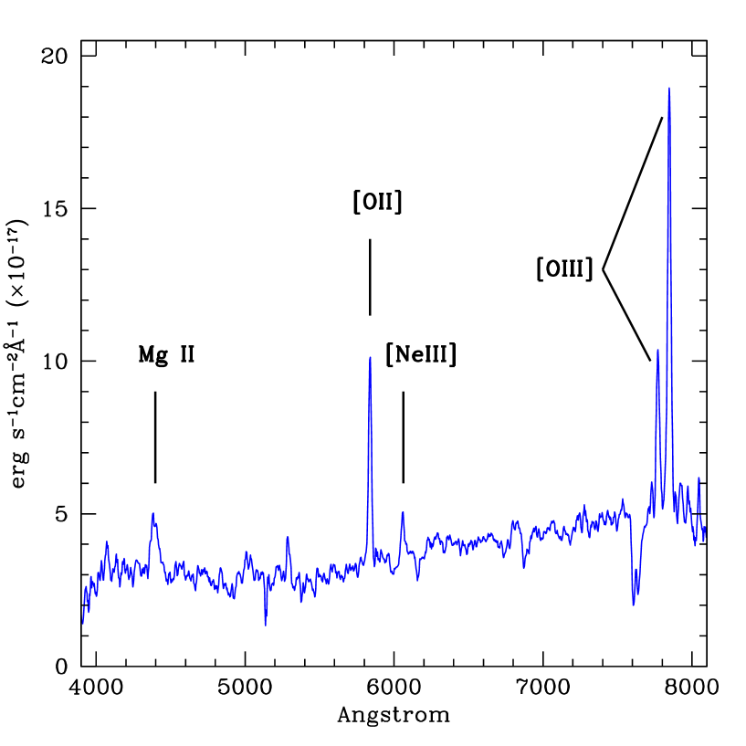
Figure 3: The optical spectrum of PKSJ 1037-2705 observed with TNG corrected for Galactic extinction. All extinction values in this paper are from Schlegel et al. (1998).

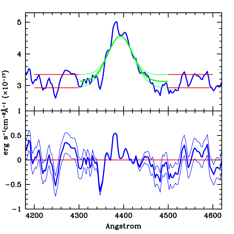
Figure 4: A closeup of the TNG spectrum of PKSJ 1037-2705 in figure 3 in the vicinity of Mg II. The horizontal red lines indicate the one sigma uncertainty in the continuum level near the Mg II BEL ($4200\AA<\lambda<4600\AA$) caused by noise. We present a range of Gaussian fits to the Mg II BEL as the continuum level is varied from the average in the band to $\pm 1\sigma$. The thick curve is the fit to the average continuum and the thin curves are the fits to the average continuum $\pm 1\sigma$. The bottom frame shows the residuals to our Gaussian fits, it looks similar to the noise in the rest of the band.

3.1 The MgII Broad Emission Line

The properties of the MgII line are important to the discussion to follow. Unfortunately, the continuum above and below the BEL is not well constrained due to significant noise and there is apparently significant noise that distorts the line shape near the peak. Since this measurement is important in the following analysis, we take special care to quantify the uncertainties in the measurement of the line strength and FWHM.

3.1.1 The Continuum Level

The major source of error in our estimates arises from uncertainties in the continuum level. Since we don’t expect any other emission lines nearby, the first thing that we can look at is the average continuum level both red-ward and blue-ward of the BEL. The errors that are induced by the noise were obtained by sampling the blue side of the Mg II BEL from 4200 $\AA$ to 4300 $\AA$ and on the red side from 4500 $\AA$ to 4600 $\AA$. We combined the red and the blue bands to estimate the local continuum level as $3.13\pm 0.21\times 10^{-17}\mathrm{ergs/s/cm^{2}/\AA}$. This band of one sigma uncertainty in the local continuum level is superimposed on the spectrum in figure 4, by two red horizontal line segments.

3.1.2 The Gaussian Fits

Figure 4 shows the single Gaussian fits to the data with the continuum set at the three levels noted in the subsection above, nominal (the average continuum level) and nominal $\pm 1\sigma$. A single Gaussian fit to the line with the continuum level fixed is given by option ”h” in IRAF splot. The IRAF generated fits have residuals that look consistent with the noise level surrounding the BEL. The FWHM values were extracted from the fitted Gaussian models after correcting for instrumental broadening which is about 20 $\AA$ measured from the sky and arclines. Our analysis indicates that the three single Gaussian fits give a range of uncertainty from the single Gaussian fit to the nominal continuum that is expressed as $L_{MgII}=1.23^{+.37}_{-.41}\times 10^{42}\mathrm{ergs/sec}$ and $\mathrm{FWHM}=4266^{+321}_{-570}$ km/s. If we consider a conservative 20% uncertainty in absolute flux calibration (this affects $L_{MgII}$, but not to the FWHM), we compute that $L_{MgII}=1.23^{+.69}_{-.57}\times 10^{42}\mathrm{ergs/sec}$.

3.1.3 The Non-Gaussian Fit

A single Gaussian fit might not be the best model of the MgII BEL in PKSJ 1037-2705. There is a significant red-ward asymmetry and there is an irregular peak possibly (the significant excess residual in figure 4) from a strong narrow line component (see section 3.5 for the evidence of a strong narrow line emissivity that is excited by the propagating jet). Another possible reason for the distortion from a smooth profile near the line peak is that the MgII line is actually a doublet. Thus, we are interested in estimating $L_{MgII}$ and the FWHM without assuming any particular parametric form (such as a single Gaussian). The IRAF option ”e” allows us to directly integrate the flux above a certain continuum level and this seems suitable for our purposes. Given the irregular line shape this direct approach is preferable to the single Gaussian model for computing $L_{MgII}$. Again, we adopt a conservative 20% uncertainty in absolute flux calibration and our direct integration for each of the three levels of continua in Figure 4 yield a spread of values about the nominal continuum estimate of $L_{MgII}=1.24^{+.58}_{-.48}\times 10^{42}\mathrm{ergs/sec}$. Which is very close to the value and uncertainty found from the single Gaussian fits in the previous subsection.

We compute the FWHM in a similar manner with the direct integration in IRAF option ”e”. We directly measured the width (in $\AA$) of the spread in the data halfway between the peak and the continuum. We corrected for instrumental broadening as in the previous subsection and found a spread in the FWHM estimates relative to the value found using the nominal continuum given by $\mathrm{FWHM}=3504^{+313}_{-799}$ km/s. The nonparametric fit and the Gaussian fits give values of the FWHM that are different at the 1.2 $\sigma$ level.

3.2 Estimating $L_{bol}$ from the Continuum Spectrum

The total bolometric luminosity of the accretion flow, $L_{bol}$, is the thermal emission from the accretion flow, including any radiation in broad emission lines from photo-ionized gas, from IR to X-ray. Since we do not have complete broadband coverage of the SED for the accretion flow, one can estimate $L_{bol}$ by means of a composite SED. The most important samples for the composite quasar spectra are the HST observations since these cover the rest frame EUV (extreme ultraviolet) region in which it was once believed that much of the quasar energy was hidden (Zheng et al, 1997). Figure 5 is a composite spectral energy distribution of a radio quiet quasar with $M_{V}=-25$ (roughly the average value in the Zheng et al (1997) HST sample). This spectrum, in combination with the broad emission lines, represents the “typical” radiative signature of a strong accretion flow onto a black hole in the absence of an FR II jet. This signature is empirical and is independent of all theoretical models of the accretion flow.

Figure 5: The composite spectral energy distribution of a quasar with $M_{V}=-25$ from the combined data of Elvis et al (1994); Zheng et al (1997); Telfer et al (2002); Laor et al (1997)

Figure 5 is a piecewise collection of power laws that approximate the individual bands. The IR and optical data are from the composite spectrum of Elvis et al (1994), the NUV (near ultraviolet) and EUV data are from the HST composites of Zheng et al (1997); Telfer et al (2002) and the X-ray portion of the composite is from Laor et al (1997). In order to compute the bolometric luminosity of the accretion flow from the composite spectral energy distribution, one can estimate (from the tables in Zheng et al (1997)and Telfer et al (2002)) that 25 percent of the total optical/UV quasar luminosity is reprocessed in the broad line region. Thus, for this $M_{V}=-25$ radio quiet composite SED, $L_{bol}=1.35\times 10^{46}\mathrm{ergs/sec}$. If one also assumes that the shape of the composite spectrum in Figure 5 is independent of quasar luminosity, a simple approximate formula is obtained that relates the k-corrected absolute visual magnitude with bolometric luminosity,

$$L_{bol}\approx 1.35\times 10^{\frac{-25-M_{V}}{2.5}}\times 10^{46}\mathrm{ergs/sec}\;.$$ (3-1)

As a more general alternative to (3.1), if $L(\nu)_{\mathrm{obs}}$ is the observed spectral luminosity at the AGN rest frame frequency, $\nu$, then $L_{bol}$ is estimated as

$$L_{bol}=1.35\frac{\nu L(\nu)_{\mathrm{obs}}}{\nu L(\nu)_{\mathrm{com}}}\times 10^{46}\mathrm{ergs/sec}\;,$$ (3-2)

where $L(\nu)_{\mathrm{com}}$ is the spectral luminosity from the composite SED.

The problem with applying (3.1) and (3.2) to PKSJ 1037-2705 is that one must subtract off the high frequency tail of the synchrotron jet. A strong contribution from the jet that masks the optical signature of the accretion flow seems likely given the best fit continuum spectral index (defined in section 2 as $F_{\nu}\propto\nu^{-\alpha}$) of $\alpha^{7500}_{4500}=3.16$ (from 7500 $\AA$ to 4500 $\AA$). In order to ascertain if the high frequency tail of this blazar component masks the optical/near UV flux from the accretion flow, we created a broadband SED (i.e., a plot of $\nu L_{\nu}$ versus $\nu$) in figure 6.

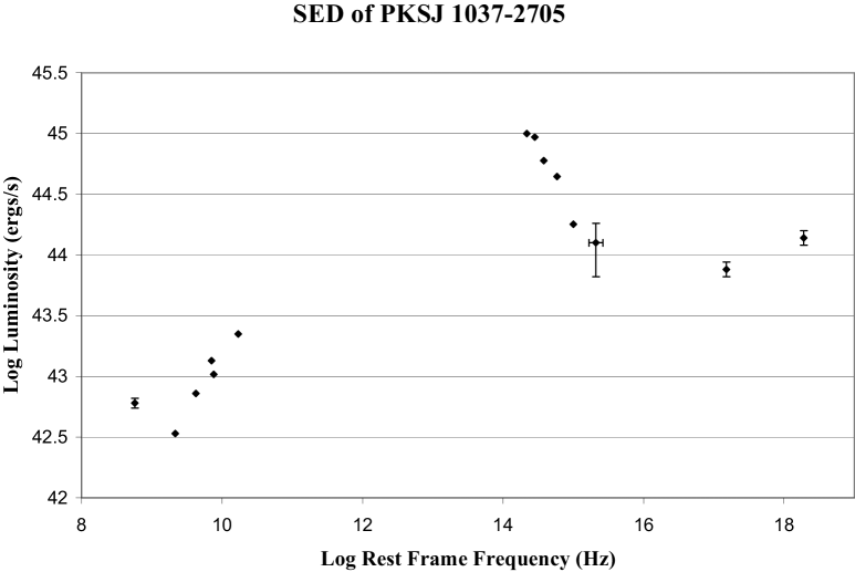
Figure 6: A broadband spectral energy distribution or SED (i.e., a plot of $\nu L_{\nu}$ versus $\nu$) for PKSJ 1037-2705. The SED is corrected for Galactic Extinction. The radio data is drawn from figure 2. The IR data is from the 2MASS survey and was accessed through MAST. The optical data is from our observations. The UV data point was from the GALEX shallow sky survey and was retrieved through MAST. The X-ray data points come from the fit to our Newton-XMM observation shown in Figure 8 (see section 4). If the error bars are smaller than the size of the data point marker then they are not shown.

Even though the data in the SED in Figure 6 were not obtained simultaneously (and blazars are highly variable), the basic shape is quite revealing. First of all, notice the peak in the SED in the IR. The peak of the SED is clearly in excess of $10^{45}\mathrm{ergs/sec}$ in the Mid-IR. The spectrum from $\lesssim 10^{10}$ Hz to $\gtrsim 10^{15}$ Hz is dominated by one component with a shape typical of the synchrotron spectrum of a blazar jet (Fossati et al, 1997). Compare this spectrum to the signature of the accretion disk, the SED for radio quiet quasars in Figure 5. The thermal SED from the accretion flow is rising from $3\times 10^{14}$ Hz to $3\times 10^{15}$, the ”big blue bump”. Conversely, the SED for PKSJ 1037-2705 is a steeply decreasing function in this same frequency range, a clear distinction from a thermal origin. The rise of the SED toward high frequency in the X-ray regime is most likely the inverse Compton emission from this very same jet (see the next section for details) which is another characteristics of blazar jets (Fossati et al, 1997). There is no evidence of a break in the synchrotron spectral index (the optically thin portion of the synchrotron peak) from the IR to the near UV (see section 3.3). The GALEX data has a large error bar associated with it, so it is not too useful. All that the GALEX data really tells us is that there is no strong strong thermal component in the UV.

The SEDs in Figures 5 and 6 indicate that the optical component from the jet is clearly much larger than that of the accretion disk. The data (the steep power law) indicates that down to at least $10^{15}$ Hz, the underlying continuum is still mostly hidden by the jet flux (see also Figure 7 and the discussion in section 3.3). Therefore, we can use Figures 5 and 6 with equation (3.2) to create an upper bound on the accretion disk luminosity. Due to the rapidly falling SED, the most stringent upper bound is formed by choosing the highest frequency UV point with relatively small errors associated with it (not the GALEX data), $\approx 10^{15}$ Hz,

$$L_{bol}=1.35\frac{\nu L(\nu)_{\mathrm{thermal}}}{\nu L(\nu)_{\mathrm{com}}}\times 10^{46}\mathrm{ergs/sec}$$

$$\ll 1.35\frac{\nu L(\nu)_{\mathrm{synchrotron}}+\nu L(\nu)_{\mathrm{thermal}}}{\nu L(\nu)_{\mathrm{com}}}\times 10^{46}\mathrm{ergs/sec}=7.64\times 10^{44}\mathrm{erg/s}\;,$$ (3-3)

where $\nu L(\nu)_{\mathrm{thermal}}$ is the contribution to the SED of PKSJ 1037-2705 from the thermal accretion flow and $\nu L(\nu)_{\mathrm{synchrotron}}$ is the synchrotron contribution to the SED (evaluated at $\approx 10^{15}$ Hz).

This upper bound is quite conservative and it is based on not finding any true signal of the accretion flow. We want to do better than this, so we dig deeper into the optical data set to find more evidence of the thermal accretion flow in the next subsections.

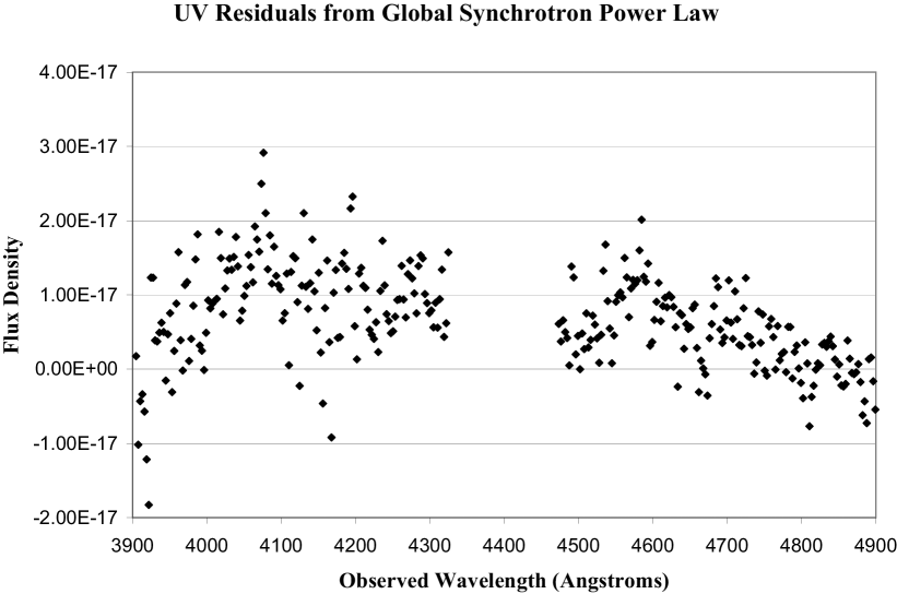
Figure 7: The residual flux density of the UV (in the quasar rest frame) continuum relative to the global synchrotron power law. A gap is left that accommodates the Mg II BEL that significantly distorts the continuum level. The best fit, steep power law, from 7500 $\AA$ down to 5000 $\AA$ that is given by $\alpha=3.39$, continues to follow the continuum very closely down to 4500 $\AA$. The figure indicates a hint of an excess of flux below 4300 $\AA$, but the results is not statistically significant. A slight excess would be indicative of a weak thermal component near 4000 $\AA$. The flux density is corrected for Galactic extinction and the units are $\mathrm{ergs/s/cm^{2}/\AA}$

3.3 Estimating $L_{bol}$ Based on the UV Excess from the Global Power Law

In order to make a better estimate than the loose upper bound in (3.3), one can look for some weak signal that is indicative of the thermal accretion flow. If there is no spectral ageing effects, one expects the optically thin portion of the jet synchrotron spectrum to be well fit by a power law. Since the optically thin synchrotron spectrum is so steep, the best chance for detecting evidence of a weak $L_{bol}$ is by looking for an inflection point in the power law spectrum blue-ward of Mg II. The farther into the UV we go, the more pronounced the thermal component becomes, based on a typical quasar spectrum from Zheng et al (1997) and the synchrotron spectral index, $F_{\lambda}(\mathrm{thermal})/F_{\lambda}(\mathrm{synchrotron})\sim\lambda^{-2.5}$.

We note that the spectral index flattens as the end point of the fit to the continuum on Figure 3 moves deeper into the UV. The values of spectral index of the best fit, de-reddened spectrum for an endpoint that goes from 5500 $\AA$ to 5000 $\AA$ to 4500 $\AA$ to 3900 $\AA$ are: $\alpha^{7500}_{5500}=3.44$, $\alpha^{7500}_{5000}=3.39$, $\alpha^{7500}_{4500}=3.16$, $\alpha^{7500}_{3900}=2.92$. It appears that there is a break in the synchrotron power law short-ward of 5000 $\AA$. This could be a sign of a UV excess above the synchrotron power law. This is not expected for a pure synchrotron source since spectral ageing, if present, actually steepens the spectrum at high frequencies. A UV excess over a pure power law fit, could be a signal of an accretion disk starting to become noticeable in the strong glare of the synchrotron jet. Unfortunately, the spectrum is noisy in the UV, as noted in the last subsection, so the excess is not statistically significant.

We explore this trend toward a UV excess over a power law by first fitting the continuum spectrum from 7500 $\AA$ to 5000 $\AA$, $\alpha^{7500}_{5000}=3.39$. We then ask the question, if this power law were extended toward the far UV, what would the residuals of the data look like, i.e., the excess. The results are plotted in Figure 7. There is evidence of a gradual trend for an excess extending into the band from 4300 $\AA$ to 3900 $\AA$. We note that in the band 4900 $\AA$ to 4500 $\AA$ that the average residual flux density is $4.5\pm 5.1\times 10^{-18}\mathrm{ergs/s/cm^{2}/\AA}$ and in the shorter wavelength band, 4300 $\AA$ to 3900 $\AA$ the average excess seems to increase to $9.1\pm 7.0\times 10^{-18}\mathrm{ergs/s/cm^{2}/\AA}$. But the excess is $\sim 1\sigma$ above the synchrotron power law, and therefore not statistically significant.

We can use this lack of statistical significance to obtain another upper bound on $L_{bol}$. If we use the flux excess in the band 4900 $\AA$ to 4500 $\AA$ to represent the value at the center of the narrow band, 4700 $\AA$ (approximately 3000 $\AA$ in the quasar rest frame), then we know that the $F_{\lambda}(\mathrm{thermal})(4700)<1.98\times 10^{-17}\mathrm{ergs/s/cm^{2}/\AA}$ at the 3 $\sigma$ level. Then (3.2) implies that $L_{bol}<5.5\times 10^{44}$ ergs/s at the 3 $\sigma$ level. This is a tighter upper bound than was found in (3.3). Similarly, one can estimate the excess from the global power law at 4100 $\AA$ (2615 $\AA$ rest frame) by averaging the excess within the band from 4300 $\AA$ to 3900 $\AA$. The flux in this band, quoted above, inserted into equation (3.2) yields $L_{bol}=2.1\pm 1.6\times 10^{44}$ ergs/s, which is consistent with the upper bound from the 4700 $\AA$ excess.

3.4 Estimating $L_{bol}$ from Broad Line Strengths

In order to constrain the accretion disk thermal luminosity, a different estimator is required. The estimator in (3.2) of bolometric luminosity of the accretion flow is a direct measurement of an accretion flow property. Thus, it is superior to using line emission to estimate the accretion flow power which is an indirect estimator. The advantage of using the line luminosity is that its strength might not be affected by the relativistic jet to first order. However, the down side of using line luminosity is that it is a second order indicator of accretion luminosity. One can use either broad lines which are $\sim$ 0.01 pc from the accretion disk or narrow lines which can occur anywhere from just outside the broad line region out to distances of $\sim 50$ kpc (Best et al, 2000a). First of all, the broad lines are closer to the photo-ionization source, so it seems that this might be a better choice. Secondly, it has been shown the the narrow lines can be created by jet propagation and might not provide a reliable diagnostic of the thermal photo-ionization source in many radio sources (Best et al, 2000b). This will discussed in more detail in the next subsection. That is why broad lines are the first choice for blazar accretion flow estimates. The method that is most commonly used for estimating $L_{bol}$ in blazars is to compare the line strengths to a composite SED (Celotti et al, 1997; Wang et al., 2004). Again, we note that the existence of a radio jet tends to produce strong narrow lines in NLRGs (Best et al, 2000b). Since the MgII line strength is so weak, subtraction of the narrow line component associated with the propagating jet is likely important to accurately estimate the broad line strength, $L_{MgII}(BEL)$, arising from the photo-ionization of BEL clouds by the accretion flow thermal emission. The composite NLRG ($z\sim 1$) spectrum produced in Best et al (2000a), indicates that the MgII narrow line strength, $L_{MgII}(NL)$ is $\approx 0.15$ of the OII line strength. Our IRAF single Gaussian (option k) fit to the spectral data indicate that $L_{OII}(NL)\approx 2.4\times 10^{42}\mathrm{ergs/sec}$. Thus, from the data reduction in section 3.1.3, $4.0\times 10^{41}\mathrm{ergs/sec}<L_{MgII}(BEL)\approx L_{MgII}-0.15L_{OII}(NL)<1.5\times 10^{42}\mathrm{ergs/sec}$. We then use the composite SED in Figure 5 combined with the HST composite quasar line strengths of Zheng et al (1997) (from which the composite SED is derived) to compute $L_{bol}\approx 204L_{MgII}(BEL)$, which is about 20% more than the Wang et al. (2004) formula ($L_{bol}\approx 168L_{MgII}(BEL)$). For PKSJ 1037-2705 this relation implies $8.2\times 10^{43}\mathrm{ergs/sec}<L_{bol}<3.1\times 10^{44}\mathrm{ergs/sec}$. This is consistent with the upper bound estimated from the optical continuum, $L_{bol}<5.5\times 10^{44}$ ergs/s, that was found in the previous subsection.

3.5 Estimating $L_{bol}$ from Narrow Line Strengths

A narrow line estimator for $L_{bol}$ could also be tried. A seminal effort in Rawlings and Saunders (1991) estimated that the total narrow line luminosity was

$$L_{NLR}\approx 9L_{OII3727}+4.5L_{OIII5007}\;.$$ (3-4)

For PKSJ 1037-2705 the lines strengths from the IRAF Gaussian fits to the spectrum in figure 3 are $L_{OII3727}\approx 2.4\times 10^{42}\mathrm{ergs/sec}$ and $L_{OIII5007}\approx 4.8\times 10^{42}\mathrm{ergs/sec}$. Thus, from equation (3.4), we estimate as per Rawlings and Saunders (1991), a narrow line luminosity of $L_{NR}\approx 4.3\times 10^{43}\mathrm{ergs/sec}$. In Rawlings and Saunders (1991) they picked an arbitrary covering factor of 0.01 for the narrow line clouds (which is likely too large by a factor of $\gtrsim 3$, see below and Willott et al. (1999)). Therefore they estimated the blue bump optical/UV luminosity, $L_{BB}=100L_{NLR}$. From the SED in Figure 5 and the broad line strengths in Zheng et al (1997), $L_{bol}\approx 1.67L_{BB}\approx 7.2\times 10^{45}\mathrm{ergs/sec}$.

Alternatively, Willott et al. (1999) claim that $L_{OIII}$ is not reliable for the estimation of $L_{bol}$ and claim that their new OII estimator is superior to their earlier efforts,

$$L_{BB}\approx 5\times 10^{3}L_{OII3727}\;.$$ (3-5)

The Willott et al. (1999) estimate gives $L_{bol}\approx 1.67L_{BB}\approx 1.9\times 10^{46}\mathrm{ergs/sec}$. The primary difference between the Willott et al. (1999) and Rawlings and Saunders (1991) is the adhoc covering factor. The revised Willott et al. (1999) value is 0.003. Note that the revised covering factor is much more compliant with the composite quasar spectrum of Francis et al (1991) that is discussed below. With the revised covering factor the narrow line luminosity implies that the flux density at 3000 $\AA$ from the ”big blue bump,” (the ionizing continuum) should be 30 times larger than what we observed in the spectrum of PKS J1037-2705. This begs the question, why is the narrow line estimator so poor for this source? Recall that Best et al (2000b) showed that $L_{NLR}$ can be from gas that was excited by shocks that are driven by the jet in radio galaxies. By using long slit spectroscopy, they found many regions of OII emitting gas that are aligned with features in the jet. A study of narrow line ratios in these aligned features indicated that the excitation state and density was explained best by the shock models. In fact, they showed that the smaller radio galaxies ($<120$ kpc) and those with broad OII lines ($\sim$ 1000 km/sec) had the majority of their narrow line gas in an ionization state that was likely excited by jet induced shocks as opposed to photo-ionization. Thus, $L_{NLR}$ is a poor diagnostic of the thermal accretion luminosity in these sources. PKSJ 1037-2705, is this type of source, a linear size $<120$ kpc and a single Gaussian fit to the OII line yields a FWHM of $\approx$ 1000 km/sec. The narrow lines are driven primarily by the jet since the photo-ionization source associated with the accretion disk is so weak as evidenced by the weak MgII BEL and the low level UV continuum emission. In order to quantify how weak the continuum ionization source is compared to the jet shock ionization source, we note that in the composite quasar spectrum of Francis et al (1991), (The Zheng et al (1997) quasar composite does not cover OII and OIII): $L_{OIII}/L_{MgII}=0.1$ and $L_{OII}/L_{MgII}=0.023$. By contrast, for PKSJ 1037-2705, we have $L_{OIII}/L_{MgII}\approx 3.9$ and $L_{OII}/L_{MgII}\approx 1.9$ (based on our best fit Gaussians). It is concluded that $L_{NLR}$ is a poor predictor of $L_{bol}$ because the ratio of the jet kinetic luminosity to the photo-ionizing luminosity is extremely high in this quasar. In fact, it is proposed that a potential method for selecting kinetically dominated quasars is to find blazars (unobscured nuclei) in which $L_{OII}/L_{MgII}>1$ and the MgII FWHM $>$ 2000 km/sec.

3.6 Summary of IR/Optical Observations

In this section we used optical observations with TNG and 2MASS archival IR data to quantify numerous characteristics of the AGN, PKSJ 1037-2705.

• PKSJ 1037-2705 is blazar with a synchrotron peak luminosity in the IR with $\nu L_{\nu}>10^{45}$ ergs/sec (see section 3.2).

• The high frequency synchrotron tail from the blazar dominates the optical and near UV luminosity created by the accretion flow (see section 3.3)

• PKSJ 1037-2705 has a Seyfert 1 thermal spectrum as evidenced by the MgII broad emission line (see section 3.1).

• Standard estimation techniques based on composite quasar spectra and the broad line strength indicate that $8.2\times 10^{43}\mathrm{ergs/sec}<L_{bol}<3.1\times 10^{44}\mathrm{ergs/sec}$. This is an order of magnitude below the Seyfert 1/QSO dividing line.

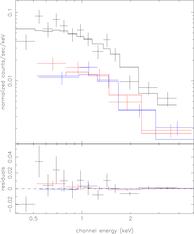
Figure 8: The X-ray spectrum from XMM-Newton. The different colors represent data for the 3 XMM-Newton cameras: black = PN, red: MOS1, blue: MOS2

4 The X-ray Observations

PKSJ1037-2705 was observed on July 3, 2004 for 18 ks with XMM-Newton. The XMM-Newton data are affected by solar flares, yielding a cleaned exposure time of only 5 ks. Following standard light-curve screening of the XMM-Newton data, spectra and response products were extracted for each EPIC camera within a 30 arcsec radius from the X-ray peak, using a surrounding 1-2.5 arcmin point-source excised annulus for background estimates. The three spectra were each accumulated in bins containing at least 25 net counts and then jointly fitted in XSPEC v11.3 using standard $\chi^{2}$ minimization. Various models were fitted with Galactic absorption (Comptonized black-body, Bremsstrahlung model, accretion disk with multiple black-body components, thermal plasma at z=0.57 and a power-law). A simple power-law absorbed by the Galaxy (ie. with no evidence of intrinsic absorption at the source) provides the best fit among the models that we tried. The spectrum is shown in Figure 8. The spectral fitting was done in the 0.4-5 keV band. We find the spectral index, $\Gamma=1.77\pm 0.20$ with reduced $\chi^{2}$=1.44 for 21 degrees of freedom (the null hypothesis probability is 0.0086). Including intrinsic absorption in the model, the best-fit hydrogen column density of such a component is only $\sim 20\%$ of the Galactic value and consistent with zero at 1 sigma (and with no improvement in fit quality). As a check of the veracity of the fit, fitting was also performed using Cash statistics on spectra binned into 5 cts/bin, but the results were generally consistent with those of $\chi^{2}$ fitting reported here.

The absorption-corrected X-ray luminosity in the quasar rest frame (the XMM-Newton band covered in Figure 8 transforms to 0.63-7.85 keV), is $2.49^{+0.42}_{-0.35}\times 10^{44}$ ergs/s. This value actually is comparable to or larger than the estimates of $L_{bol}$ that was computed from the broadline strength, a common signature of a blazar. Archival ROSAT data of this source (also known as IXO 37) was extrapolated with $\Gamma=1.7$ (similar to our value) in Colbert and Ptak (2002) to compute the 2 -10 keV intrinsic luminosity. After correcting for the incorrect redshift in Colbert and Ptak (2002) and extrapolating our best-fit model to to 2 -10 keV, we find that the source was $\approx 2.5$ times more luminous at the time of the ROSAT observations. This type of large X-ray variation (a factor of a few, in time frames of years or shorter) is characteristic of a blazar.

5 Discussion

In this article, we established the following

1. PKSJ 1037-2705 is a blazar based on radio core dominance, a flat radio core spectrum, the large radio and X-ray variability, a steep optical spectrum and an inordinately large X-ray luminosity (relative to the UV and $L_{MgII}$).

2. PKSJ 1037-2705 has the extended radio flux typical of an FR II quasar.

3. PKSJ 1037-2705 is a broadline object that is likely to have an accretion flow luminosity an order of magnitude weaker than a quasar, i.e. it is a Seyfert 1 galaxy.

4. PKSJ 1037-2705 is likely to be kinetically dominated based on the spread in the estimated values of $\overline{Q}$ and $L_{bol}$ that were determined in sections 2 and 3, respectively: $4.3/3.1=1.4<\overline{Q}/L_{bol}<9.3/0.82=11.3$.

The proof that Seyfert 1 AGN can host FRII jets is based on a few anecdotal examples. Note that these objects are distinct from broad line radio galaxies (BLRGs). The Mid-IR observations of Ogle et al (2006) indicate that FRII BLRGs have nuclei with quasar level luminosity which are often obscured by dusty gas. Even though Seyfert 1 FRII radio sources might not be exceptionally rare, demonstrating the existence of a single object explicitly is extremely challenging. For example, Ogle et al (2006) suggest that their weak Mid-IR subsample of NLRGs are hosted by low luminosity AGN, i.e., Seyfert 1 level thermal luminosity. However, Cleary et al. (2007) would argue that the absorbing columns to these NLRGs is so dense that even the IR can not escape and there is still a hidden quasar buried inside.

The existence of Seyfert 1 nuclei in FRII sources is important for understanding the connection between the accretion flow and the jet power, with two possible implications. Firstly, the kpc scale emission that was used to compute $\overline{Q}$ was ejected from the AGN $\sim 10^{6}-10^{7}$ years earlier than $L_{bol}$ was created (Willott et al., 1999; Blundell and Rawlings, 2000). It is not clear if there should be a strong connection between the present value of $L_{bol}$ and the value of $L_{bol}$ $\sim 10^{6}-10^{7}$ years ago. On the one hand, strong variability has been detected in the thermal emission from Seyfert 1 nuclei with changes of a factor of 5 in luminosity in weeks or months (Antonucci and Cohen, 1983; Alloin et al, 1988). The observation of this type of variability has led researchers such as Alloin et al (1988); Cutri et al (1985); Antonucci (1988) to conclude that the variability time scale for $L_{bol}$ can not be related to the thermal and viscous time scales of an accretion disk. On the other hand, there is evidence that some high redshift quasars have been active for $>10^{7}$ years based on the $\mathrm{He}^{+}$ Lyman $\alpha$ ”proximity effect” (Jakobsen et al, 2003). The “proximity effect” arises when a large bubble forms about the quasar in which helium is highly ionized by the quasar. One can use the size of the bubble to estimate the amount of time it would take for the photo-ionizing source to ionize the extended region. However, one must be cautious to extrapolate this result to much less luminous Seyfert 1 galaxies and it does not provide evidence that the photo-ionization source was steady within a factor of 10 during the entire $10^{7}$ years. With all this being said, it would be a huge stretch in reasoning to assume that in spite of the large short term variations that have been observed in some Seyfert 1 galaxies that $L_{bol}$ is constant to within a factor of 10 over $10^{7}$ years. Hence, there does not seem to be any compelling observation or underlying reason why the two quantities, $\overline{Q}$ and $L_{bol}$ should be related, even if the accretion flow drives the jet.

Alternatively, the existence of Seyfert 1 nuclei in FR II radio sources could mean that the accretion rate is not that strongly coupled to the jet power. Unfortunately, as a consequence of the Doppler boosting there is no reliable contemporaneous estimate of $Q(t)$ that can be used to test the latter hypothesis (see the discussion in section 2.2). In the context of our previous work, we have now reported on 3 Seyfert 1 galaxies that have $\overline{Q}\geq L_{bol}$, PKSJ 1037-2705 ($L_{bol}\gtrsim 10^{44}$ ergs/s), 3C 216 ($L_{bol}\gtrsim 10^{44}$ ergs/s) and PKS 1622-253 ($L_{bol}\approx 2\times 10^{45}$ ergs/s) (Punsly, 2006; Punsly et al, 2005). All three have convincing evidence of a contemporaneous powerful jet and a weak (Seyfert 1 level) $L_{bol}$. The evidence for an active jet in PKSJ 1037-2705 is a powerful peak in the synchrotron SED, $\nu L_{\nu}>10^{45}$ ergs/s, in the IR based on archival 2MASS data. Similarly, the two epochs of X-ray data indicates that it is plausible that the inverse Compton peak of the SED in the X-ray band, (0.3 keV - 10 keV in the rest frame) exceeds $10^{45}$ ergs/s during the high states (ROSAT epoch). 3C 216 has a strong peak in the synchrotron SED $>10^{46}$ ergs/s. PKS 1622-253 is one of the strongest EGRET gamma ray sources, the gamma-ray apparent luminosity has a time average value of $\sim 10^{47}\mathrm{ergs/sec}$ and flares at $\sim 10^{48}\mathrm{ergs/sec}$ (Hartman et al, 1999). This circumstantial evidence tends to support the interpretation that even weak (Seyfert 1 level) accretion flows onto a black hole can produce a central engine for FRII jets. Thus, our study is supportive of the Ogle et al (2006) interpretation of the weak Mid-IR, FRII NLRG subsample, they contain low luminosity nuclei.

Finally, we comment on the conjecture in Boroson (2002); Maccarone et al (2003) that these three Seyfert I galaxies, possessing a large jet power (at the FRII level), are not unusual objects, based on the small value of $L_{bol}/L_{Edd}$ in Seyfert 1 galaxies compared to QSOs (Sun and Malkan, 1989). This conclusion is a natural consequence of the claim in Boroson (2002); Maccarone et al (2003) that a small value of $L_{bol}/L_{Edd}$ is conducive to jet formation. The implication is that Seyfert I galaxies (with their relatively low values of $L_{bol}/L_{Edd}$ compared to QSOs), possessing FR II radio power, should be a common state of AGN activity. However, this conjecture seems difficult to reconcile with the sparsity of known FR II level extended emission associated with broad line nuclei with Seyfert 1 level luminosity in optically selected samples (there is not a single example in the New General Catalog, Palomar-Green Survey or the Markarian catalog). Such a simple proposal is also at odds with the anecdotal case of PKS 0743$-$67 that was studied in detail in Punsly and Tingay (2005) for just this reason. PKS 0743$-$67 is an example of a quasar that has an ultra-luminous accretion flow, $L_{bol}>2\times 10^{47}\mathrm{ergs/s}$, and has a very high Eddington rate, $L_{bol}/L_{Edd}\approx 1$. The jet kinetic luminosity was conservatively estimated at $\overline{Q}=4.1\times 10^{46}$ ergs/sec which is 2.5 times that of Cygnus A. However, this was a conservative lower bound and the radio data also supports $\overline{Q}\approx 10^{47}$ ergs/sec, i.e one of the most powerful radio sources in the known Universe. Furthermore, PKS 0743$-$67 is presently active as evidenced by the powerful ($>1Jy$) unresolved VLBI radio core. A low Eddington ratio is not likely to be determinant to FRII jet production.

References

- Alloin et al (1988) Alloin, D., Pelat, D., Phillips, M., Whittle, M, 1985, ApJ 288 205
- Andernach et al (1988) Andernach, H. et al, 1988, A& AS 73 265
- Antonucci (1988) Antonucci, R., 1988 Supermassive black holes in Proceedings of the Third George Mason Astrophysics Workshop, Fairfax, VA, Oct. 14-16, 1986 (Cambridge University Press, New York) p. 26-38
- Antonucci and Cohen (1983) Antonucci, R. and Cohen, R., 1983, ApJ 271 564
- Antonucci and Ulvestad (1985) Antonucci, R. and Ulvestad, J., 1985, ApJ 294 185
- Barthel et al (1990) Barthel, P., Tytler, D., Thompson, B. 1990, Astron. and Astrophys. Sup. 82 339
- Best et al (2000a) Best, P., R ttgering, H., Lehnert, M. 2000 MNRAS 311 1
- Best et al (2000b) Best, P., R ttgering, H., Lehnert, M. 2000 MNRAS 311 23
- Blundell and Rawlings (2000) Blundell, K., Rawlings, S. 2000, AJ 119 1111
- Boroson (2002) Boroson, T. 2002, ApJ 565 78
- Bridle et al (1994) Bridle, A. et al 1994, AJ 108 766
- Bridle and Perley (1984) Bridle, A. and Perley, R. 1984, Annu. Rev. Astron. Astrophys. 22 319
- Celotti et al (1997) Celotti, A., Padovani and Ghisellini, G. 1997, MNRAS 286 415
- Clarke (1999) Clarke, T.E. 1999, PhD Dissertation University of Toronto.
- Cleary et al. (2007) Cleary, K.; Lawrence, C. R.; Marshall, J. A.; Hao, L.; Meier, D 2007, ApJ 660 117
- Colbert and Ptak (2002) Colbert, E., Ptak, A. 2002, ApJS 143 25
- Cutri et al (1985) Cutri, R., Wisniewski, W., Rieke, G., Lebofsky, M. 1985, ApJ 296 423
- Elvis et al (1994) Elvis, M. et al 1994, ApJS 95 1
- Fossati et al (1997) Fossati, G.; Celotti, A.; Ghisellini, G.; Maraschi, L 1997 MNRAS 289 136
- Francis et al (1991) Francis, P. et al 1991, ApJ 373 465
- Gutierrez (2006) Gutierrez, C. 2006 ApJL, 640, 17
- Hartman et al (1999) Hartman, R.. et al 1999, ApJS 123 79
- Jakobsen et al (2003) Jakobsen, P., Jansen, R., Wagner, S., Reimers, D. 2003, A & A 397 891
- Kellermann et al (1969) Kellermann, K. I., Pauliny-Toth, I. I. K., Williams, P. J. S. 1969 ApJ 157 1
- Kuehr, H et al. (1981) Kuhr, H., Witzel, A., Pauliny-Toth, I.I.K., Nauber, U. 1981, A & AS 45, 367
- Laor et al (1997) Laor, A. et al 1997, ApJ 477 93
- Lind and Blandford (1985) Lind, K., Blandford, R. 1985, ApJ 295 358
- Maccarone et al (2003) Maccarone, T., Gallo, E., Fender, R. 2003 MNRAS 345, L19
- Ogle et al (2006) Ogle, P., Whysong, D. and Antonucci, R. 2006 ApJ 647, 161
- Punsly (1995) Punsly, B. 1995, AJ 109 1555
- Punsly (2001) Punsly, B. 2001, Black Hole Gravitohydromagnetics (Springer-Verlag, New York)
- Punsly (2005) Punsly, B. 2005, ApJL 623 9
- Punsly (2006) Punsly, B. 2006, ApJL 651 17
- Punsly and Tingay (2005) Punsly, B., Tingay, S. 2005, ApJL 633 L89
- Punsly et al (2005) Punsly, B., Rodriguez, L., Tingay, S., Cellone, S. 2005, ApJL 633 L93
- Rawlings and Saunders (1991) Rawlings, S., Saunders, R. 1991, Nature 349, 138
- Schlegel et al. (1998) Schlegel, D. J., Finkbeiner, D. P. & Davis, M. 1998, ApJ 500 525
- Sun and Malkan (1989) Sun, W.H., Malkan, M. 1989, ApJ 346 68
- Telfer et al (2002) Telfer, R., Zheng, W., Kriss, G., Davidsen, A. 2002, ApJ 565 773
- Vestergaard and Peterson (2006) Vestergaard, M. and Peterson, B. 2006, ApJ 641 689
- Wang et al. (2004) Wang, J.-M., Luo, B, Ho, L. 2004, ApJL 615 9
- Willott et al. (1999) Willott, C., Rawlings, S., Blundell, K., Lacy, M. 1999, MNRAS 309 1017
- Zheng et al (1997) Zheng, W. et al 1997, ApJ 475 469