Discussing Cosmic String Configurations in a Supersymmetric Scenario without Lorentz Invariance

Abstract

The main goal of this work is to pursue an investigation of cosmic string configurations focusing on possible consequences of the Lorentz-symmetry breaking by a background vector. We analyze the possibility of cosmic strings as a viable source for fermionic Cold Dark Matter particles. Whenever the latter are charged and have mass of the order of $10^{13}GeV$, we propose they could decay into usual cosmic rays. We have also contemplated the sector of neutral particles generated in our model. Indeed, being neutral, these particles are hard to be detected; however, by virtue of the Lorentz-symmetry breaking background vector, it is possible that they may present an electromagnetic interaction with a significant magnetic moment.

I Introduction

The mechanisms for breaking symmetries in theories of fundamental Physics may yield many interesting spectral relations among particles. In Quantum Field Theory, important invariances appear in connection with the Standard Model for Particle Physics. These symmetries are the Lorentz, CPTCPT and Supersymmetry (SUSY) Weinberg invariances. Lorentz- and CPT-symmetry breakingsColloday98 ; Kostelecky89 can occur if we consider processes at energy scales close to the Planck mass Carroll:1989vb ; Kostelecky99 . In Quantum Electrodynamics, there is a number of works that present constraints on the Lorentz-symmetry violating parameters Jacobson:2003bn ; Stecker:1992wi . One of the most important processes for which the breaking of Lorentz symmetry may be measurable is related to high-energy $\gamma$-rays from extragalactic sources. The idea in the works that treat this question is that the $\gamma$-rays are absorbed during their interaction with the low-energy photons of intergalactic radiation Stecker:1992wi ; Stecker:1998ib ; there occurs annihilation into electron-positron pairs in intergalactic space. This sort of physical process imposes constraints on the Lorentz-invariance violation parameters, which can also yield bounds from the astrophysical testsStecker:1992wi ; Stecker:2004xm ; Stecker:2004vm .

To study these phenomena, some authors proposed alternative models that can describe Lorentz-symmetry breakings and their effectsKostelecky89 ; Carroll:1989vb ; Kostelecky95 . The other symmetry we study in our work is supersymmetry (SUSY), which is the main ingredient of new theories, such as the Physics Beyond the Standard Model; it appears as a viable framework that solves some problems of the Standard Model and gives us possible candidates to Dark Matter (DM). The astronomical evidence for additional, non-luminous matter, or dark matter, strengthens our motivations to consider SUSY. Another motivation to adopt SUSY is the fact that this symmetry appears as the main ingredient of String TheoryGreen87 . In the Minimally Supersymmetric Standard Model (MSSM), the breaking of SUSY is soft, which is an attractive way of solving the hierarchy problem and linking the electroweak scale to physics close to the Planck scale. This soft SUSY breaking can be related with the Lorentz-invariance violation (LIV) in the study of the vortex superfluidsFerreira:2008zz , where the LIV is realized by a Kalb-Ramond fieldDavis:1989gn .

The Kalb-Ramond and dilaton fields appear in heterotic string theory and can couple to the Yang-Mills-Maxwell-Chern-Simons field as the result of a quantum effect. The Kalb-Ramond field can play the role of the background field in Majumdar:1999jd ; Maity:2004he . In another context, vortex configurations may be studied in the brane-world framework Braga:2004ns and present important results in a supersymmetric scenario Morris:1995wd ; Davis:1997bs ; Ferreira:2000pi ; Ferreira:2002mg ; NunesFerreira:2005if . These motivations are the basis for this work, where we consider a rather general set of background fields that induce LIV in connection with possible supersymmetric cosmic string configurations. Structures like cosmic strings Vilenkin:1981zs ; Hiscock:1985uc ; Gott:1984ef ; Garfinkle:1985hr ; Hindmarsh:1994re ; Vilenkin1 ; Kibble:1980mv , probably produced during phase transitions Kibble:1976sj , appear in some Grand-Unified gauge theories and carry a huge energy density Hindmarsh:1994re . They have been studied to provide a possible origin for the seed density perturbations which became the large scale structure of the Universe observed today Sato:1986pd . These fluctuations would leave their imprint in the Cosmic Microwave Background Radiation (CMBR) that would act as seeds for structure formation and, then, as builders of the large-scale structures in the Universe Turok:1985tt . However, they have presently been discarded as the only responsible for structure formation. They have re-acquired renewed phenomenological interest in connection with String Theory Kibble:2004hq ; Polchinski:2004ia . They may also help to explain the most energetic events in the Universe, such as ultra-high-energy cosmic raysBhattacharjee:1989vu ; Bhattacharjee:1991zm ; MacGibbon:1989kk above the Greisen-Zatsepin-Kusmin (GZK) cut-off, that lies on energies of the order of 5 x $10^{10}$ GeV Kuzmin:1998kk . In this work, we analyze possible consequences of supersymmetric cosmic strings interactingBezerra:2004qv ; Ferreira:2002mg with a vector background responsible for the Lorentz breaking effect Belich:2003fa . This scenario may yield consequences to particle creation and this is an issue we devote special attention to in the present paper.

The outline of this work is as follows: in Section II, we start by presenting a simple model with a Lorentz-symmetry breaking contribution formulated in terms of superfields. In Section III, we study vortex configurations and we discuss the physical implications of this Lorentz-symmetry violation. We also analyze the potential, the magnetic flux and the currents induced by LIV. In Section IV, we compute the propagator for the excitations in the gauge sector of the model and comment on the role of the Lorentz-symmetry breaking additional terms. Section V is devoted to the study of the fermionic charged fields that can be ejected from cosmic strings. We consider the possibility that these fields may be interpreted as the responsible for charged Cold Dark Matter (CDM) particles. In Section VI, we set up the part of the model that accounts for the neutral particles that may appear as (neutral) CDM particles. We give here special room to the discussion of the possible magnetic moment interactions of these neutral particles. Finally, in Section VII, we draw our General Conclusions with a discussion on phenomenological aspects of our model.

II Supersymmetric Cosmic string model with Lorentz-Invariance Violation

In this Section, we present the general features of a supersymmetric model that may produce cosmic string configurations with LIV. To accommodate cosmic strings in a supersymmetric context, we need a family of chiral scalar superfields, $\Phi_{i}(\phi_{i},\xi_{i},G_{i})$. These superfields contain the complex physical scalar fields, $\phi_{i}$, their fermionic partners, $\xi_{i}$, and complex auxiliary fields, $G_{i}$; they can be written as $\theta$-expansions according to the parameterization below:

$$\Phi_{i}=e^{-i\theta\sigma^{\mu}\bar{\theta}\partial_{\mu}}[\phi_{i}(x)+\theta^{a}\xi_{ia}(x)+\theta^{2}G_{i}(x)]\,,$$ (1)

where the label $i$ represents the flavours of the superfields needed to the correct description of the cosmic string. The other fundamental ingredient for a cosmic string configuration is the gauge field, $H_{\mu}$. To accommodate this field, we consider a gauge superfield, ${\cal V}_{{}_{\!H}}$, which also contains a fermionic gauge partner, $\chi$, and a real auxiliary field, $D$. The superfield ${\cal V}_{{}_{\!H}}$ is already assumed to be in the Wess-Zumino gauge, with a $\theta$- expansion as follows:

$${\cal V}_{{}_{\!H}}=\theta\sigma^{\mu}\bar{\theta}H_{\mu}(x)+\theta^{2}\bar{\theta}\bar{\chi}(x)+\bar{\theta}^{2}\theta\chi(x)+\theta\bar{\theta}^{2}D(x)\,.$$ (2)

The cosmic string Lagrangian, ${\cal L}_{{}_{CS}}$, that is $U(1)$-gauge symmetry invariant and presents $N=1$ supersymmetry is

$${\cal L}_{{}_{CS}}=\bar{\Phi}_{i}\,e^{{}^{\!2q_{i}\,{\cal V}}}\!\!\Phi_{i}|_{{}_{\theta\theta\bar{\theta}\bar{\theta}}}\!\!+\alpha\,{\cal H}^{\alpha}\,{\cal H}_{\alpha}|_{{}_{\theta\theta}}\!\!\,+W|_{{}_{\theta\theta}}+h.c.,$$ (3)

where $\alpha$ is a real parameter, h.c. is the Hermitian conjugate, and the field-strength superfield, ${\cal H}^{a}$, is written as ${\cal H}^{a}=-\frac{1}{4}\bar{\cal D}^{2}{\cal D}^{a}{\cal V}_{{}_{H}}$. The supersymmetry covariant derivatives are given as ${\cal D}_{a}=\partial_{a}-i\sigma^{\mu}_{a\dot{a}}\bar{\theta}^{\dot{a}}\partial_{\mu}$ and $\bar{\cal D}_{\dot{a}}=-\partial_{\dot{a}}+i\theta^{a}\sigma^{\mu}_{\dot{a}a}\partial_{\mu},$ where the $\sigma^{\mu}$-matrices read as $\sigma^{\mu}\equiv({\bf 1};\sigma^{i})$, the $\sigma^{i}$’s being the Pauli matrices.

To realize the U(1)-gauge symmetry breaking responsible for the cosmic string vacuum, we consider a superpotential, $W$, as given by

$$W=\beta\Phi_{0}\Big{(}\Phi_{+}\Phi_{-}-\eta^{2}\Big{)},$$ (4)

where $\eta$ and $\beta$ are real parameters. Then, we consider in (3),$\,\,i=0,\,+,\,-$   with $q_{0}=0$ related to the neutral superfield, $q_{+}=1$ associated to the chiral supermultiplet and $q_{-}=-1$ to the anti-chiral supermultiplet.

In a scenario with SUSY, this structure is sufficient to obtain a cosmic string Morris:1995wd ; but, in our case, we wish to study this phenomenon in connection with LIV. This fact changes the cosmic string configuration giving us new features.

Models with LIV without SUSY have been already studiedBezerra:2004qv ; nevertheless, if we consider events that occur in the early universe, as the cosmic string formation, we need to include SUSY. In this analysis, we consider the cosmic string in the presence of the supersymmetric version of the Maxwell-Chern-Simons term; so, we need another gauge superfield, ${\cal V}_{{}_{\!A}}$, that has the same form as the one given in eq.(2) and is also taken in the Wess-Zumino gauge:

$${\cal V}_{{}_{\!A}}=\theta\sigma^{\mu}\bar{\theta}A_{\mu}(x)+\theta^{2}\bar{\theta}\bar{\lambda}(x)+\bar{\theta}^{2}\theta\lambda(x)+\theta\bar{\theta}^{2}\tilde{D}(x)\,.$$ (5)

Also, we have to add a dimensionless chiral superfield, $\Omega(\omega,\psi,I)$, given by

$$\Omega=e^{-i\theta\sigma^{\mu}\bar{\theta}\partial_{\mu}}[\omega(x)+\theta^{a}\psi_{a}(x)+\theta^{2}I(x)],$$ (6)

which carries a complex scalar field, $\omega$, a fermionic partner, $\psi$, and an auxiliary field, $I$. The Lagrangian that accommodates the LIV term reads as below

$${\cal L}_{{}_{MCS}}={\cal F}^{a}{\cal F}_{a}|_{{}_{\theta\theta}}+{\cal H}^{a}{\cal F}_{a}\Omega|_{{}_{\theta\theta}}+h.c.\,.$$ (7)

The Lagrangian ${\cal L}_{{}_{MCS}}$ is written in terms of a field-strength superfield, ${\cal F}^{a}=-\frac{1}{4}\bar{\cal D}^{2}{\cal D}^{a}{\cal V}_{{}_{A}}$, that accommodates the electromagnetic field, $A_{\mu}$, the photino, $\lambda$, and a real auxiliary field, $\tilde{D}$.

For a detailed description of the component fields and degrees of freedom displayed in (5), the reader is referred to the paper of ref. Belich:2003fa . As it can be readily checked, this action is invariant under Abelian gauge and SUSY transformations Ferreira:2002mg . The SUSY transformations act upon the string bosonic configuration, and the fermionic zero-mode excitations turn out to be:

$$\begin{array}[]{ll}\xi^{\pm}_{a}=i\sqrt{2}\sigma^{\mu}_{a\dot{a}}\bar{\varepsilon}^{\dot{a}}D_{\mu}\phi^{\pm}+\sqrt{2}\varepsilon_{a}G^{\pm},\\ \\ \xi^{0}_{a}=i\sqrt{2}\sigma^{\mu}_{a\dot{a}}\bar{\varepsilon}^{\dot{a}}\partial_{\mu}\phi^{0}+\sqrt{2}\varepsilon_{a}G^{0},\\ \\ \chi_{a}=\sigma^{\mu\nu}_{a\dot{a}}\varepsilon^{\dot{a}}H_{\mu\nu}+i\varepsilon_{a}D,\\ \\ \psi_{a}=i\sqrt{2}\sigma^{\mu}_{a\dot{a}}\bar{\varepsilon}^{\dot{a}}\partial_{\mu}\omega,\\ \\ \lambda_{a}=\sigma^{\mu\nu}_{a\dot{a}}\varepsilon^{\dot{a}}F_{\mu\nu}+i\varepsilon_{a}\,\tilde{D}.\end{array}$$ (8)

The physical interpretation of the Lagrangian ${\cal L}_{MCS}$ is that the dimensionless superfield, $\Omega$, represents the background that can give us information about the early universe when cosmic strings were formed. In this context, LIV can become an important ingredient for cosmic string appearance. This cosmic string is superconducting and has a different characteristic with respect to the usual and Witten’s cosmic strings Witten:1986qx .

III Cosmic String Interactions in a Framework with LIV

In this Section, let us analyze cosmic string configurations. We study the equations of the motion and show that it is possible to find solutions in our model. In components, we have a $U(1)\times U(1)^{\prime}$ mixing-term Foot:1994vd , which can be diagonalised by considering the following field reshufflings:

$$H_{\mu} \rightarrow (1-\rho^{2})^{-1/2}H_{\mu}$$ (9)

$$A_{\mu} \rightarrow A_{\mu}-\rho(1-\rho^{2})^{-1/2}H_{\mu},$$ (10)

where we write the real part of $\omega$ as $(\omega+\omega^{*})\equiv\rho$. The mixing - term comes from the Lagrangian of equation (7).

In this work, we choose the condition $\alpha+2\rho=1$ to specify the background field configurations for the $\omega$-field, in such a way that we have $\rho={\rm constant}$. The constant $\rho$ is, in our analysis, a physical parameter and cannot be completely scaled away in the presence of the Lorentz-breaking interaction. In string theory Green87 , the $\rho$-field may exhibit interaction with the gauge potential; here, with a LIV environment, it freezes at a constant value in the background.

For the on-shell version of the present model, we have the bosonic Lagrangian:

$$L_{B}=2D_{\mu}\phi[D^{\mu}\phi]^{*}-\frac{1}{4}H_{\mu\nu}H^{\mu\nu}-\frac{1}{4}F_{\mu\nu}F^{\mu\nu}$$

$$\!\!\!+{1\over 2}(1\!-\!\rho^{2})^{{}^{\!\!-1\!/2}}\!\epsilon^{{}^{\mu\alpha\beta\nu}}\!\!\!\!\!\!\!v_{\mu}\,H_{\alpha\beta}\Big{[}\!\rho(1-\rho^{2})^{{}^{\!\!-1/2}}H_{\nu}\!+\!A_{\nu}\!\Big{]}\!-\!U,$$ (11)

where the Lorentz-symmetry breaking term that contains the antisymmetric part of $\omega$ is written as $(\omega-\omega^{*})=i\Delta$. The form of $\Delta$ is fixed in terms of the LIV parameter, since we define $v_{\mu}=i\partial_{\mu}\Delta$ as a constant. This ansatz for $\rho$ and $v_{\mu}$ is possible whenever we consider a static background.

The bosonic fields, in polar coordinates, may be parameterized as (axially symmetric ansatz):

$$\phi_{0} = 0$$ (12)

$$\phi_{{}_{+}} = \phi_{-}^{*}=f(r)e^{in\theta}=\phi$$ (13)

$$H_{\mu} = H_{\theta}(r)\delta_{\mu}^{\theta}$$ (14)

$$G_{\pm} = D=0$$ (15)

$$G_{0} = \mu\Big{(}\eta^{2}-f(r)^{2}\Big{)}\,,$$ (16)

where $G_{\pm}$, $D$ and $G_{0}$ are the auxiliary fields introduced in the previous section.

We impose as boundary conditions:

$$\begin{array}[]{lllll}f(r)=0&r=0&&f(r)=\eta&r\rightarrow\infty.\\ \end{array}$$ (17)

The gauge covariant derivative is:

$$D_{\mu}\phi=[\partial_{\mu}+ie(1-\rho^{2})^{-1/2}H_{\mu}]\phi.$$ (18)

The potential turns out to be given by:

$$U = \beta(\bar{\phi}_{+}\bar{\phi}_{-}-\eta^{2})(\phi_{+}\phi_{-}-\eta^{2})$$ (19)

$$+ \beta\bar{\phi}_{0}\phi_{0}\Big{(}\bar{\phi}_{+}\phi_{+}+\bar{\phi}_{-}\phi_{-}\Big{)}\,.$$

With the ansatz (16) for the cosmic string, $U$ can be split according to:

$$U=\beta\,\Big{(}|\phi|^{2}-\eta^{2}\Big{)}^{2}.$$ (20)

Now, let us analyze the charge induced by the Lorentz-symmetry breaking in the cosmic string core. The field equations imply that $\phi$ and $H_{\mu}$ are solutions to the following differential equation:

$$\partial_{\mu}\partial^{\mu}\phi+e^{2}(1-\rho^{2})^{-1}H_{\mu}H^{\mu}-{\partial V(\phi)\over\partial\phi}=0,$$ (21)

which yields,

$${1\over r}{d\over dr}\Big{(}r{df\over dr}\Big{)}-\Big{[}\Big{(}{n\over r}-e(1-\rho^{2})^{-1/2}H\Big{)}^{2}-2\beta(f^{2}-\eta^{2})\Big{]}f=0.$$ (22)

The equations for the gauge fields are given by

$$\partial_{\mu}H^{\mu\nu}={\cal J}^{\nu}+{\cal J}_{top}^{\nu},$$ (23)

where the 4-dimensional current density, ${\cal J}_{\nu}$, is related to the cosmic string fields according to

$${\cal J}_{\mu}=-ie\left[\phi^{*}\partial_{\mu}\phi-\phi(\partial_{\mu}\phi)^{*}\right]+2e(1-\rho^{2})^{-1}|\phi|^{2}H_{\mu}.$$ (24)

Let us consider the Lorentz-symmetry violating vector, $v_{\mu}=(0,0,0,v)$, being so chosen that, whenever $\mu=z$, it is connected with the charge, $Q$. The ${\cal J}_{top}^{\mu}$ is the topological current, with the extra gauge field, $A_{\mu}$, given by

$${\cal J}_{top}^{\mu}=-(1-\rho^{2})^{-1/2}\epsilon^{\mu\nu\alpha\beta}v_{\nu}F_{\alpha\beta}.$$ (25)

The equation for the gauge potential along the angular component is

$$B_{z}={1\over r}{d\over dr}\Big{(}rH(r)\Big{)}$$ (26)

$${dB_{z}\over dr}+2e(1-\rho^{2})^{-1/2} \Big{[}{n\over r}+e(1-\rho^{2})^{-1/2}H\Big{]}f^{2}\,+$$

$$v(1-\rho^{2})^{-1/2}E=0\,,$$ (27)

where the magnetic field is defined as $B_{k}=\epsilon_{ijk}H^{ij}$ and the electric field is given by $F_{0r}=-E$. The equation for the gauge field, $A_{\mu}$, is given by

$$\partial_{\mu}F^{\mu\nu}=(1-\rho^{2})^{-1/2}\epsilon^{\nu\kappa\alpha\beta}v_{\kappa}H_{\alpha\beta};$$ (28)

In terms of the magnetic and electric fields, we have

$${1\over r}{d\over dr}\Big{(}r\,E(r)\Big{)}=v(1-\rho^{2})^{-1/2}B_{z}(r).$$ (29)

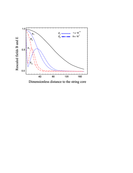
Figure 1:  In this graph, we plot the behavior of the electric and   magnetic   fields   of   the  cosmic   string with mixing parameter, $\rho$. We consider $v=0.03$.

The magnetic flux is quantized as below:

$$\phi_{Mag} = \oint H_{i}rdx^{i}=-2\frac{\pi}{e}n(1-\rho^{2})^{1/2}.$$ (30)

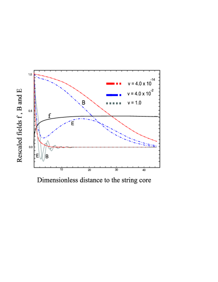
Figure 2: In this graph, the point curve shows the behavior of the cosmic string with parameter  $v$ . The  solid   curve   is the ordinary cosmic string solution, i.e.  $v=0$   and   $\rho=0$. The parameter of the other curves is $\rho=10^{-11}$.

The region of validity for $\rho$ ( $\rho<1$, actually, $\rho$ is a very small parameter) ensures that the magnetic flux is non-vanishing and conserved, as depicted in Figure 1, in terms of the variation of the parameter $\rho$.

The solution to this problem is the change of the cosmic string configuration to include $A_{t}\neq 0$ in the $v_{z}$ case. In Figure 2, we plot the solution of the electric field, E, magnetic field, B, and scalar, f, in terms of the dimensionless radial coordinate. This graph is important to analyze the convergence of the fields, which illustrates the stability of our cosmic string solution. The comparison between our solutions and the ordinary cosmic string solution shows that an electric field appears and falls off as $1/r$, when $r\rightarrow\infty$. This is compatible with the vortex configuration.

It is relevant to analyze the fact that this cosmic string is charged and the symmetry whose breaking is involved here is Lorentz invariance, different from the Witten’s superconducting cosmic string. In the Witten’s framework, the superconductivity is given by the breaking of the $U(1)$ gauge symmetry in the core, which gives the current and the preserved gauge symmetry in the vacuum that responds for the long-range behavior of the electromagnetic field, $F_{\mu\nu}$. This mechanism includes two complex scalar fields that interact through a more complicated potential. In our approach, the unique gauge symmetry that is broken is the U(1)-group concerned to the cosmic string configuration; for this reason, the potential includes only the cosmic string field, $\phi$.

IV The Cosmic String Propagator

Another important ingredient that we have to analyze are the propagator of the gauge-field sector. There is a mixing of the $A_{\mu}$-and $H_{\mu}$ -potentials given by the LIV term. The poles of the propagator and their corresponding residues allow us to infer about the spectrum of spin-0 (longitudinal) and spin-1 (transverse) excitations: we have to be sure that neither tachyonic poles nor ghost-like states are present in the model. Specially now, that both $A_{\mu}$ and $H_{\mu}$ are mixed and an external background vector, $v^{\mu}$, appears that may, in general, yield massive poles, we must guarantee that the gauge-field sector is not plagued by unphysical modes.

With this purpose, we parameterize $\phi$ as $\phi=[{\tilde{\phi}}(x)^{\prime}+\eta]e^{i\Sigma(x)}$, where $\tilde{\phi}^{\prime}$ is the quantum fluctuation around the ground state, $\eta$. We concentrate on the bosonic Lagrangian in terms of the physical fields, $\tilde{\phi}^{\prime}$, $H_{\mu}$ and $A_{\mu}$, and we adopt the unitary gauge for the broken U(1)’-factor (associated to $H_{\mu}$). This gauge choice $\Sigma=0$ is in perfect agreement with the Wess-Zumino gauge adopted in the eq. (2) of Section 2. By fixing this gauge, we remove away compensating fields introduced by SUSY. We are still left with the usual gauge freedom, so that we still have the freedom to fix the unitary gauge. For the sake of reading off these propagator, we refer to the bosonic Lagrangian (11). We first write it in a more convenient form:

$${\cal L}=\frac{1}{2}\sum_{\alpha\beta}{\cal A}^{\alpha}{\cal O}_{\alpha\beta}{\cal A}^{\beta},$$ (31)

where ${\cal A}^{\alpha}=(A^{\mu},H^{\mu},A^{\mu})$ and ${\cal O}_{\alpha\beta}$ is the wave operator. We notice that $\Sigma$ mixes with $A^{\mu}$. However, we adopt the t’Hooft $R_{\xi}$-gauge and they decouple from each other. So, the $\Sigma-\Sigma$ propagator can be derived independently from the propagator for the ($A^{\mu},H^{\mu}$) sector. We apply the usual procedure to invert the operator ${\cal O}^{-1}_{\alpha\beta}$ in order to find the gauge-field propagator of this problem.

To read off the gauge-field propagator, we shall use an extension of the spin-projection operator formalism presented in Kuhfuss:1986rb . The new aspect in this work is that, describing the LIV terms in connection with the cosmic string fields, we have to add other new operators coming from the Lorentz-symmetry breaking terms and the cosmic string interactions. Then, we need the usual two operators, $\Theta_{\mu\nu}$ and $\Gamma_{\mu\nu}$, being respectively, the transverse and longitudinal projection operators, given by $\Theta_{\mu\nu}=\eta_{\mu\nu}-\Gamma_{\mu\nu}$, and $\Gamma_{\mu\nu}=\frac{\partial_{\mu}\partial_{\nu}}{\Box}$. In order to find the inverse of the wave operator, let us calculate the products of operators for all non-trivial combinations involving the projectors. The relevant multiplication rules are listed in Table I, where the new spin operator coming from the Lorentz breaking sector is $\Omega_{\mu\nu}$, defined in terms of Levi-Civita tensor as

Table 1: Multiplicative table for spin operators

	$\theta^{\alpha}_{\hskip 8.5359pt\nu}$	$\Gamma^{\alpha}_{\hskip 8.5359pt\nu}$	$\Omega^{\alpha}_{\hskip 8.5359pt\nu}$	$\Lambda^{\alpha}_{\hskip 8.5359pt\nu}$	$\Sigma^{\alpha}_{\hskip 8.5359pt\nu}$	$\Sigma^{\hskip 8.5359pt\alpha}_{\nu}$
$\theta_{\mu\alpha}$	$\theta_{\mu\nu}$	0	$\Omega_{\mu\nu}$	$\Lambda_{\mu\nu}-\frac{\lambda}{\Box}\Sigma_{\mu\nu}$	$\Sigma_{\mu\nu}-\lambda\Gamma_{\mu\nu}$	0
$\Gamma_{\mu\alpha}$	0	$\Gamma_{\mu\nu}$	0	$\frac{\lambda}{\Box}\Sigma_{\nu\mu}$	$\lambda\Gamma_{\mu\nu}$	$\Sigma_{\nu\mu}$
$\Omega_{\mu\alpha}$	$\Omega_{\mu\nu}$	0	$f_{\mu\nu}$	0	0	0
$\Lambda_{\mu\alpha}$	$\Lambda_{\mu\nu}-\frac{\lambda}{\Box}\Gamma_{\mu\nu}$	$\frac{\lambda}{\Box}\Sigma_{\mu\nu}$	0	$v^{2}\Lambda_{\mu\nu}$	$v^{2}\Sigma_{\mu\nu}$	$\lambda\Lambda_{\mu\nu}$
$\Sigma_{\mu\alpha}$	0	$\Sigma_{\mu\nu}$	0	$\lambda\Delta_{\mu\nu}$	$\lambda\Sigma_{\mu\nu}$	$\Lambda_{\mu\nu}\Box$
$\Sigma_{\alpha\mu}$	$\Sigma_{\nu\mu}-\lambda\Gamma_{\mu\nu}$	$\lambda\Gamma_{\mu\nu}$	0	$v^{2}\Sigma_{\nu\mu}$	$v^{2}\Box\Gamma_{\mu\nu}$	$\lambda\Sigma_{\nu\mu}$

$$\Omega_{\mu\nu}=\epsilon_{\alpha\beta\mu\nu}v^{\alpha}\partial^{\beta},$$ (32)

and the operator $f_{\mu\nu}$, that we find by squaring $\Omega$, gives us

$$f_{\mu\nu}\equiv\Omega_{\mu\alpha}\Omega^{\alpha}_{\nu}=M_{7}\Gamma_{\mu\nu}+M_{8}\Lambda_{\mu\nu}+M_{9}\Sigma_{\mu\nu},$$ (33)

so that we have to define other operators such as

$$\Sigma_{\mu\nu} = v_{\mu}\partial_{\nu},$$ (34)

$$\lambda\equiv\Sigma_{\mu}^{\mu} = v_{\mu}\partial^{\mu},$$ (35)

$$\Lambda_{\mu\nu} = v_{\mu}v_{\nu}.$$ (36)

The operators $\Sigma_{\mu\nu}$ and $\lambda$ project the longitudinal part of a vector field along the $v^{\mu}$-direction, while $\Lambda_{\mu\nu}$ projects the whole vector field (longitudinal plus transverse part) along $v^{\mu}$.

We write below the explicit expressions for the propagator we are interested in:

$$<AA> = \frac{i}{M_{1}}\Theta_{\mu\nu}+\frac{i}{(M_{2}-M_{3}^{2}M_{4}^{-1}M_{7})}\Gamma_{\mu\nu}$$ (37)

$$- \frac{i}{M_{3}^{2}M_{4}^{-1}M_{8}}\Lambda_{\mu\nu}-\frac{i}{M_{3}^{2}M_{4}^{-1}M_{9}}\Sigma_{\mu\nu}\;$$

$$<HH> = \frac{i}{M_{4}}\Theta_{\mu\nu}+\frac{i}{(M_{5}-M_{3}^{2}M_{1}^{-1}M_{7})}\Gamma_{\mu\nu}$$ (38)

$$- \frac{i}{M_{3}^{2}M_{1}^{-1}M_{8}}\Lambda_{\mu\nu}-\frac{i}{M_{3}^{2}M_{1}^{-1}M_{9}}\Sigma_{\mu\nu}\;,$$

where the first term in both equations is the transverse part of the propagator, the second is the longitudinal part, the other two terms are related with the LIV, and $M_{1},...,M_{9}$ are quantities that read as the following expressions:

$$\begin{array}[]{lll}M_{1}=M_{8}=\Box,\hskip 8.5359ptM_{2}=-\frac{1}{\epsilon}\Box,\hskip 8.5359ptM_{3}=M_{6}=-{1\over(1-\rho^{2})^{1/2}},\\ \\ M_{4}=\frac{1}{2}\Box+2e^{2}(1-\rho^{2})\eta^{2},\hskip 14.22636ptM_{5}=2e^{2}(1-\rho^{2})\eta^{2},\\ \\ M_{7}=[-v^{2}\Box-\lambda^{2}],\hskip 14.22636ptM_{9}=\frac{\lambda}{2},\end{array}$$ (39)

where $\lambda$ is the momentum space expression for the operator (35).

In our notation, $<AA>$ represents the propagator for the gauge field $A_{\mu}$, and $<HH>$ stands for the propagator between the gauge fields $H_{\mu}$ that is connected with the cosmic string.

By analyzing the $<AA>$ propagator, we can show that the transverse part is given by $M_{1}$. It has a trivial pole, then this field describes a massless excitation and its $U(1)$- symmetry does not break down. This analysis is important because it gives us information on the range of the field. The fact that the field $A_{\mu}$ presents an exact $U(1)$ gauge symmetry gives us the interpretation that is associated to a long-range interaction. This propagator displays a pole at $k^{2}=0$ also in the $\Lambda_{\mu\nu}$-sector, which indicates the presence of a massive excitation along the background $v^{\mu}$. This is not the case for the $\Lambda_{\mu\nu}$-sector of the $<HH>$ propagator. It is interesting to notice that the $<AA>$ - and - $<HH>$ propagator present a pole of the type $v^{\mu}k_{\mu}=0$, which points to an excitation that propagates orthogonally to $v^{\mu}$.

As for the propagator (38), the transverse part presents a mass given by $4e^{2}(1-\rho^{2})\eta^{2}$. We notice that this mass presents a parameter $\rho$, connected with the LIV. This parameter is very important for the understanding of the range of the gauge field $H_{\mu}$. If $\rho=1$, the field is free, but the vortex disappears because, in this limit, we have, by eq. (30), a zero magnetic flux. Then, the parameter $\rho$ is important to give us a fine-tuning of the interaction.

V Fermionic Charged Particles from Cosmic String configuration

In this Section, we shall consider the sector of fermionic excitations that propagate on the background settled down by the bosonic cosmic string configuration. Let us consider the Lagrangian for the $\Xi$-field:

$${\cal L}_{CC}=i\bar{\Xi}_{+}\gamma^{\mu}D_{\mu}\Xi_{+}+i\bar{\Xi}_{-}\gamma^{\mu}D_{\mu}\Xi_{-}+i\bar{\Xi}_{0}\gamma^{\mu}\partial_{\mu}\Xi_{0},$$ (40)

where ${\cal L}_{CC}$ is the Lagrangian piece that contains the charged fermionic fields written down in terms of four-component Majorana spinors as follows:

$$\Xi_{\pm}\equiv\Xi_{1}\pm i\Xi_{2}$$ (41)

where $\Xi_{1}$ and $\Xi_{2}$ have the form $\Xi(x)=\Big{(}\begin{array}[]{ll}\xi_{a}(x)\\ \bar{\xi}^{\dot{a}}(x)\end{array}\Big{)}$. The gauge covariant derivatives are:

$$D_{\mu}\Xi_{+} = (\partial_{\mu}+ie(1-\rho^{2})^{-1/2}H_{\mu})\Xi_{+},$$

$$D_{\mu}\Xi_{-} = (\partial_{\mu}-ie(1-\rho^{2})^{-1/2}H_{\mu})\Xi_{-}\,.$$ (42)

The Yukawa Lagrangian is given as below:

$$\begin{array}[]{ll}{\cal L}_{Y}=&\beta\,\,\Big{(}\phi_{-}\Xi_{0}\Xi_{+}+\phi_{+}\Xi_{0}\Xi_{-}\Big{)}+h.c..\end{array}$$ (43)

We propose that the fermionic solution, in the inner region of the cosmic string, displays, in cylindric coordinates, the form:

$$\Xi_{i}=\Xi(r,\theta)_{i}e^{\alpha_{i}(z-t)},$$ (44)

where $\alpha_{i}(z-t)$ represents the left-moving superconducting currents flowing along the string at the speed of light, because in the core of the cosmic string, the fermions do not have mass, because $\phi_{i}=0$. In this case, the Lagrangian (40) gives us the zero-modes inside the string.

The other important aspect are the currents inside the string: they are conserved currents. One of them is the Noether current, given by

$${\cal J}_{{}_{(\Xi)}}^{a} = -{e\over(1-\rho^{2})^{1/2}}\Big{[}\bar{\Xi}_{+}\gamma^{a}\Xi_{+}-\bar{\Xi}_{-}\gamma^{a}\Xi_{-}\Big{]}.$$ (45)

This current only involves the fermionic SUSY partners of the cosmic string scalar fields. Inside the string, SUSY is broken in the range of $10^{11}-10^{13}$ GeV and there appears a fermionic current. This current, described by (45), can be in the $z$-direction, carrying an electric field, $E_{z}$. The dynamics of the current can be given by

$${dJ_{z}\over dt}={e^{2}\over(1-\rho^{2})}E_{z}\,.$$ (46)

We notice that the variation of the current has a dependence on the LIV parameter $\rho$. This current grows until produced particles are ejected from the cosmic string. These charged fermions particles acquire masses from the breaking of the U(1) gauge symmetry where the scalar cosmic string field $<|\phi_{\pm}|>$ has a vacuum value, $\eta$. The fermionic particle masses studied here are described by Yukawa’s term that reads after a gauge symmetry breaking

$${\cal L}_{Y}=\beta\,\,\eta\,\Big{(}\Xi_{0}\Xi_{+}+\Xi_{0}\Xi_{-}\Big{)}.$$ (47)

The physical interpretation of these particles could be formulated in the context ultra-energetic cosmic rays, above the Greisen-Zatsepin-Kuzmin cut-off of the spectrum, and we propose that they are originated from decays of superheavy long-living $CDM$-particles. These particles may have been produced in the early Universe from our cosmic string after inflation and may constitute a considerable fraction of Cold Dark Matter. These $CDM$ particles are supersymmetric fermionic particles that can be produced by some cosmic string mechanism. In some cases, induced isocurvature density fluctuations can leave an imprint in the anisotropy of cosmic microwave background radiation. The fermionic mass outside the string is given by (47): $M_{F}=\beta\,\eta$. We consider that the masses of these $CDM$ particles are of the order of $10^{13}$ GeV Kuzmin:1998kk and they are in a range compatible with supersymmetric scales. We have a coupling parameter, $\mu=10^{-3}$, and the cosmic string gauge field breaking parameter is of the order of $\eta=10^{16}$ GeV, that corresponds to the energy scale at the end of the inflation. This parameter can work as a constraint for the coupling constant of the superpotential term (4).

VI Fermionic Neutral Particles and Magnetic Moment Coupling

Now, we pay attention to the neutral particles present in our model and we focus on their magnetic moment interaction. These particles, like the charged particles of the previous Section, can be considered as Dark Matter. According to astronomical observations, there is clear evidence for additional, non-luminous matter (or dark matter) in gravitational interactions; we however do not still understand their nature, for instance, their masses and other quantum numbers. Therefore, it is important to analyze their properties and other possible interaction mechanisms they may exhibit. These particles are a relic of the early Universe (for this reason, in many cases their masses are very heavy), but there are alternative production scenarios, where very light particles can also act as Cold Dark Matter, as in the case of the axion Sikivie:2007qm . In our framework, we have SUSY scales that give us huge masses. However, these particles are hard be detected. It is possible to have some ways to do that. The particles considered here are non-charged, but can interact electromagnetically to some extent. For instance, the neutron is a neutral particle with a significant magnetic moment. Thus, we wish to work on the possibility that dark matter has a small electromagnetic coupling via its magnetic moment and this moment is a by-product of LIV, as we shall see.

The Lagrangian that contains the non-charged fields is:

$${\cal L}_{NC}=i\bar{X}\gamma^{\mu}\partial_{\mu}X+i\bar{\Lambda}\gamma^{\mu}\partial_{\mu}\Lambda\,,$$ (48)

where the spinor $X$ is a partner of $H_{\mu}$ and $\Lambda$ is a partner of the $A_{\mu}$,

$$\begin{array}[]{ll}X(x)=\Big{(}\begin{array}[]{ll}\chi_{a}(x)\\ \bar{\chi}^{\dot{a}}(x)\end{array}\Big{)}&\Lambda(x)=\sqrt{2}\Big{(}\begin{array}[]{ll}\lambda_{a}(x)\\ \bar{\lambda}^{\dot{a}}(x)\end{array}\Big{)}\,.\end{array}$$ (54)

We consider the expansion of the fermionic field $\Psi$ in the $\Lambda$ and $X$ basis as $\Psi=g\Lambda+g\rho X$, where the background field is given by

$$\Psi(x)=\Big{(}\begin{array}[]{ll}\psi_{a}(x)\\ \bar{\psi}^{\dot{a}}(x)\end{array}\Big{)}\,.$$ (55)

Adopting the basis for the physical gauge fields defined as in (10), we find that the neutral fields have an interesting coupling to the electromagnetic fields as below:

$${\cal L}_{I}=\Big{(}g\bar{\Lambda}\sigma^{\mu\nu}H_{\mu\nu}\Lambda+g\rho\bar{X}\sigma^{\mu\nu}F_{\mu\nu}X\Big{)}\,,$$ (56)

where $g$ is a real constant and the term responsible for the decay is

$${\cal L}_{decay}=g\bar{\Lambda}\sigma^{\mu\nu}F_{\mu\nu}X\,.$$ (57)

These fields present a mass term given by the coupling to the background density according to

$${\cal L}^{M}_{NC}=-m(\bar{X}X+\bar{\Lambda}\Lambda)\,.$$ (58)

where $m={8\rho^{2}|\Psi|^{2}\over(1-\rho^{2})^{2}}$. The Lagrangian (58) has the form of a mass term, where $|\Psi|^{2}$ can be interpreted as the density. To understand the interaction Lagrangians (48), (56) and (58), let us analyze the equation of the motion for the fermionic field $X$, given by:

$$\Big{(}i\gamma^{\mu}\partial_{\mu}+\rho\sigma_{\mu\nu}F^{\mu\nu}-M\Big{)}X=0,$$ (59)

where the mass particle is $M={m\over g\rho}$. We have now a physical interpretation for the behavior of these neutral particles in connection with the magnetic moment. Aharonov and Casher proposed, in 1984, an experiment where they showed that there exists a phenomenon, in analogy with the Aharonov-Bohm effect, that involves the dynamics of a magnetic dipole moment in the presence of an external electric field Aharonov:1984xb . We can show, with the help of the Lagrangian (56), that the cosmic string may be the source of the magnetic moment Bertone:2004pz of the neutral supersymmetric massive particles that interact with the electric field, giving us an equation of motion as in (59).

By analysing the electric and magnetic fields generated in our system, we find that the electric field outside the string is given by $E=-\frac{Q}{4\pi\epsilon_{0}r}$   for   $v_{z}\neq 0$ and $B_{z}=-\frac{\mu_{0}J}{4\pi r}$   for   $v_{t}\neq 0$. This result shows that the breaking of Lorentz symmetry yields both electric charge and current associated to the magnetic flux related with the z-projection in the electric case and t-projection in the magnetic case of the violating background vector. The interesting point to be analyzed here is the fact that the parameters $\mu_{0}$ and $\epsilon_{0}$ are related with the Lorentz-symmetry breaking parameter $\rho$, that represents the fixed background. Considering only the electric field and using the same procedure, we find that the magnetic moment in an external electric field gives us the Hamiltonian $H_{{}_{NR}}=(1/2M)\Big{(}{\vec{p}}-{\vec{E}}\times{\vec{\mu}}\Big{)}^{2}-\mu^{2}E^{2}/M\,,$ where, in the second term, there appears the correction induced by the electric dipole moment. The notation we used is ${\mu}=2\rho={\kappa\,e\over 2M}$, which, for consistency, gives as ${m\over g}={\kappa e\over 4}$, where $\kappa$ is the gyromagnetic ratio.

VII General Conclusions and Remarks

In this work, we have contemplated the possibility of formation of a cosmic string configuration in a supersymmetric scenario where there is Lorentz- symmetry violation. We have also considered its implications in a cosmological context. As we have discussed, the astronomical observations provide compelling evidence for additional, non-luminous matter, or dark matter, and the most plausible theory that govern these particles should be based on SUSY. On the other hand, there are evidences that the high-energy events in our Universe can point to a LIV and there are observations of the excess emission amplitude that gives us an agreement in temperature density fluctuation with the cosmic microwave background, showing that the Universe may be different from what one has proposed until now Fixsen:2009xn ; Seiffert:2009xs ; Kogut:2009xv . It may happen that, in some era of the Universe, LIV should not be discarded. With these implications, it is very important to analyze the theoretical and experimental aspects of this scenario.

We show that, with our model, it is possible to have a discussion on the fermionic charged supersymmetric massive particles. These particles appear as SUSY partners in the same chiral scalar superfields that accommodate the cosmic string scalar fields. Their masses are originated from their Yukawa couplings, and so they are connected with the cosmic string breaking scale, given by the scalar field vacuum expectation value, $\eta$, in the order of $10^{16}$ GeV. In our approach, we use the Yukawa coupling constant ($\mu$) of the order of $10^{3}$ to give us particles with an energy compatible with $10^{13}$ GeV. The parameter $\mu$ can be interpreted as the responsible for the fine tuning and can be adjusted with the experimental data.

We have chosen this mass scale to take into account the experimental evidences of the highly energetic cosmic rays, above the GZK cut-off of the spectrum, that could be originated from decays of superheavy long-living X-particles Kuzmin:1998kk . These particles could be produced in the early Universe from vacuum fluctuations during (and, in our case, after) the inflation, when the cosmic string formation and the SUSY breaking took place. There is another fine tuning parameter in our model, given by the LIV, that we have denoted by $\rho$; it parameterize the magnetic flux and has non-trivial consequences on the analysis of the range of the gauge fields.

Another contribution of this work is the study of the magnetic moment of the neutral dark matter particles. This magnetic moment could be a way to detect them. The idea is that these particles can present electromagnetic interactions to some extent. We know of particles of the SM in a similar situation; for instance, the neutron, that does not present electric charge, but has a significant magnetic momentGardner:2008yn . In our model, we show that the Aharonov-Casher may occur and an electric interaction with the magnetic moment of neutral particles takes place. This is a feature of the LIV consequences in a supersymemtric framework.

In our discussion, we may consider that our model can describe the axino. After a period of inflationary expansion, the Universe established a full thermal equilibrium at the temperature $T_{R}$. In the Large Hadron Colider (LHC) measurements, we can determine the temperature, $T_{R}$, in terms of the mass of the dark matter particles. Astrophysical and cosmological observations give us the determination of the relic density of the cold dark matter in the range of the $0,104\pm 0,009$ Spergel:2006hy . These results may be adopted to impose constraints on the LIV parameters. This question is under consideration and we shall be reporting on it in a forthcoming paper (CA ).

Acknowledgments:

CNF and JAH-N would like to express their gratitude to CNPq-Brasil for the invaluable financial support.

References

- (1) J. S. Schwinger, Phys. Rev. 82, 914 (1951); G. Lüders and B. Zumino, Phys. Rev. 106, 385, (1957): For experimental tests to see: R. M. Barnett et al. [Particle Data Group], Phys. Rev. D 54, 1 (1996); B. Schwingenheuer et al., Phys. Rev. Lett. 74, 4376 (1995); R. Carosi et al. [NA31 Collaboration], Phys. Lett. B 237, 303 (1990).
- (2) S. Weinberg, The Quantum Theory of Fields, Vol. III, Cambridge University Press, Cambridge, 2000; J. Wess and J. Bagger, Supersymmetry and Supergravity, 2nd ed., Princeton University Press, Princeton, 1992.
- (3) D. Colladay and V. A. Kostelecky, Phys. Rev. D 55, 6760 (1997) Phys. Rev. D 58, 116002 (1998)
- (4) V. A. Kostelecky and S. Samuel, Phys. Rev. D 40, 1886 (1989); V. A. Kostelecky and R. Potting, Nucl. Phys. B 359, 545 (1991).
- (5) V. A. Kostelecky, ed, CPT and Lorentz Symmetry, World Scientific, Singapore, 1999.
- (6) S. M. Carroll, G. B. Field and R. Jackiw, Phys. Rev. D 41, 1231 (1990).
- (7) F. W. Stecker, O. C. de Jager and M. H. Salamon, Astrophys. J. 390, L49 (1992).
- (8) T. A. Jacobson, S. Liberati, D. Mattingly and F. W. Stecker, Phys. Rev. Lett. 93, 021101 (2004)
- (9) F. W. Stecker and M. H. Salamon, Astrophys. J. 512, 521 (1999)
- (10) F. W. Stecker and S. T. Scully, Astropart. Phys. 23, 203 (2005)
- (11) F. W. Stecker, Int. J. Mod. Phys. A 20, 3139 (2005) [arXiv:astro-ph/0409731].
- (12) V. A. Kostelecky, R. Potting, Phys. Lett. B 381, 89 (1996); Phys Rev D 51, 3923 (1996);
- (13) Green M, Schwarz J. and Witten E, ”Superstring Theory, vol 2 (Cambridge: Cambridge University Press), (1987).
- (14) C. N. Ferreira, J. A. Helayel-Neto and W. G. Ney, Phys. Rev. D 77, 105028 (2008).
- (15) R. L. Davis and E. P. S. Shellard, Phys. Rev. Lett. 63, 2021 (1989).
- (16) P. Majumdar and S. SenGupta, Class. Quant. Grav. 16, L89 (1999) [arXiv:gr-qc/9906027].
- (17) D. Maity, P. Majumdar and S. SenGupta, JCAP 0406, 005 (2004) [arXiv:hep-th/0401218].
- (18) N. R. F. Braga and C. N. Ferreira, JHEP 0503, 039 (2005) [arXiv:hep-th/0410186].
- (19) C. N. Ferreira, C. F. L. Godinho and J. A. Helayel-Neto, New J. Phys. 6, 58 (2004) [arXiv:hep-th/0205035].
- (20) J. R. Morris, Phys. Rev. D 53, 2078 (1996) [arXiv:hep-ph/9511293].
- (21) S. C. Davis, A. C. Davis and M. Trodden, Phys. Lett. B 405, 257 (1997) [arXiv:hep-ph/9702360].
- (22) C. N. Ferreira, M. B. D. Porto and J. A. Helayel-Neto, Nucl. Phys. B 620, 181 (2002)
- (23) C. Nunes Ferreira, H. Chavez and J. A. Helayel-Neto, PoS WC2004, 036 (2004) [arXiv:hep-th/0501253].
- (24) T. W. B. Kibble, Phys. Rept. 67, 183 (1980).
- (25) A. Vilenkin, Phys. Rev. D 23, 852 (1981).
- (26) W. A. Hiscock, Phys. Rev. D 31, 3288 (1985).
- (27) J. R. I. Gott, Astrophys. J. 288, 422 (1985).
- (28) D. Garfinkle, Phys. Rev. D 32, 1323 (1985).
- (29) M. B. Hindmarsh and T. W. B. Kibble, Rept. Prog. Phys. 58, 477 (1995) [arXiv:hep-ph/9411342].
- (30) A.Vilenkin and E.P.S.Shellard, Cosmic Strings and other Topological Defects (Cambridge University Press, 1994).
- (31) T. W. B. Kibble, J. Phys. A 9, 1387 (1976).
- (32) Y. Sato, Prog. Theor. Phys. 75, 914 (1986).
- (33) N. Turok and R. H. Brandenberger, Phys. Rev. D 33, 2175 (1986).
- (34) T. W. B. Kibble, arXiv:astro-ph/0410073.
- (35) J. Polchinski, arXiv:hep-th/0412244.
- (36) P. Bhattacharjee, Phys. Rev. D 40, 3968 (1989).
- (37) P. Bhattacharjee, C. T. Hill and D. N. Schramm, Phys. Rev. Lett. 69, 567 (1992).
- (38) J. H. MacGibbon and R. H. Brandenberger, Nucl. Phys. B 331, 153 (1990).
- (39) V. Kuzmin and I. Tkachev, Phys. Rev. D 59, 123006 (1999) [arXiv:hep-ph/9809547]. Bezerra:2004qv
- (40) V. B. Bezerra, C. N. Ferreira and J. A. Helayel-Neto, Phys. Rev. D 71, 044018 (2005) [arXiv:hep-th/0405181].
- (41) H. Belich, J. L. Boldo, L. P. Colatto, J. A. Helayel-Neto and A. L. M. Nogueira, Phys. Rev. D 68, 065030 (2003) [arXiv:hep-th/0304166].
- (42) E. Witten, In *Chicago 1986, Proceedings, Relativistic Astrophysics* 606-620.
- (43) R. Foot, X. G. He, H. Lew and R. R. Volkas, Phys. Rev. D 50, 4571 (1994)
- (44) R. Kuhfuss and J. Nitsch, Gen. Rel. Grav. 18, 1207 (1986).
- (45) P. Sikivie, D. B. Tanner and K. van Bibber, Phys. Rev. Lett. 98, 172002 (2007) [arXiv:hep-ph/0701198].
- (46) Y. Aharonov and A. Casher, Phys. Rev. Lett. 53 (1984) 319.
- (47) G. Bertone, D. Hooper and J. Silk, Phys. Rept. 405, 279 (2005) [arXiv:hep-ph/0404175].
- (48) D. J. Fixsen et al., arXiv:0901.0555 [astro-ph.CO].
- (49) M. Seiffert et al., arXiv:0901.0559 [astro-ph.CO].
- (50) A. Kogut et al., arXiv:0901.0562 [astro-ph.GA].
- (51) S. Gardner, Phys. Rev. D 79, 055007 (2009) [arXiv:0811.0967 [hep-ph]].
- (52) D. N. Spergel et al. [WMAP Collaboration], Astrophys. J. Suppl. 170, 377 (2007).
- (53) J. E. Kim, A. Masiero and D. V. Nanopoulos, Phys. Lett. B 139, 346 (1984).
- (54) C. N. Ferreira, L. A. S. Nunes, C. A. Almeida and J. A. Helayel-Neto, work in progress.