Calculating free energy profiles in biomolecular systems from fast non-equilibrium processes

Abstract

Often gaining insight into the functioning of biomolecular systems requires to follow their dynamics along a microscopic reaction coordinate (RC) on a macroscopic time scale, which is beyond the reach of current all atom molecular dynamics (MD) simulations. A practical approach to this inherently multiscale problem is to model the system as a fictitious overdamped Brownian particle that diffuses along the RC in the presence of an effective potential of mean force (PMF) due to the rest of the system. By employing the recently proposed FR method [I. Kosztin et al., J. of Chem. Phys. 124, 064106 (2006)], which requires only a small number of fast nonequilibrium MD simulations of the system in both forward and time reversed directions along the RC, we reconstruct the PMF: (1) of deca-alanine as a function of its end-to-end distance, and (2) that guides the motion of potassium ions through the gramicidin A channel. In both cases the computed PMFs are found to be in good agreement with previous results obtained by different methods. Our approach appears to be about one order of magnitude faster than the other PMF calculation methods and, in addition, it also provides the position dependent diffusion coefficient along the RC. Thus, the obtained PMF and diffusion coefficient can be used in a suitable stochastic model to estimate important characteristics of the studied systems, e.g., the mean folding time of the stretched deca-alanine and the mean diffusion time of the potassium ion through gramicidin A.

I Introduction

The study of the structure-function relationship of biomolecular systems often requires to follow their dynamics with almost atomic spatial resolution on a macroscopic time scale, which is beyond the reach of current all atom molecular dynamics (MD) simulations. A typical example is molecular and ion transport through channel proteins Roux (2002). Indeed, in order to determine the forces that guide the diffusion of molecules across the channel one needs to know with atomic precision the structure of the channel protein-lipid-solvent environment. However, the duration of the permeation process across the channel occurs on a time scale (e.g., $\mu$s to ms) that may exceed by several orders of magnitude the time scale of several tens of nanoseconds currently attainable by all atom molecular dynamics (MD) simulationsBecker et al. (2001). Whenever the dynamic properties of interest of such a system can be described in terms of a small number of reaction coordinates (RCs) then a practical approach to this inherently multiscale problem is to model the system as fictitious overdamped Brownian particles that diffuse along the RCs in the presence of an effective potential of mean force (PMF) that describes their interaction with the rest of the system.

Recently we have proposed an efficient method for calculating simultaneously both the PMF, $U(R)$, and the corresponding diffusion coefficient, $D$, along a RC, $R$, by employing a small number of fast nonequilibrium MD simulations in both forward (F) and time reversed (R) directions Kosztin et al. (2006). The efficiency of this method, referred to as the FR method, was demonstrated by calculating the PMF and the diffusion coefficient of single-file water molecules in single-walled carbon nanotubes Kosztin et al. (2006). The obtained results were found to be in very good agreement with the results from other PMF calculation methods, e.g., umbrella sampling Frenkel and Smit (2002); Roux (1995); Torrie and Valleau (1977).

To further test its viability, in this paper we apply the FR method to investigate the energetics of two well-studied exemplary systems, i.e., (i) the helix-to-coil transition of deca-alanine in vacuum, and (ii) the transport of $K^{+}$ ions in the gramicidin A (gA) channel protein, inserted in a fully solvated POPE lipid bilayer. In each case we seek to calculate the PMF as a function of a proper RC, i.e., the end-to-end distance ($R$) of deca-alanine and the position ($z$-coordinate) of the potassium ion along the axis of the gA channel. The computed PMFs are found to be in good agreement with previous results obtained by using either the Jarzynski equality Park and Schulten (2004); Park et al. (2003) or the umbrella sampling method Frenkel and Smit (2002); Roux (1995); Torrie and Valleau (1977). However, compared to these PMF calculation methods our approach is about one order of magnitude faster and, in addition, also provides the position dependent diffusion coefficient along the RC. Thus, by employing the computed PMF and diffusion coefficient in a suitable stochastic model we could estimate important characteristics of the studied systems, e.g., the mean folding time of the stretched deca-alanine and the mean first passage time of $K^{+}$ through the gA channel.

The remaining of the paper is organized as follows. To make the presentation self-contained, in Sec. II a brief description of the FR method is provided, along with the theory used to analyse our results. The study of deca-alanine is described in Sec. III, while that of $K^{+}$ transport in the gA channel in Sec. IV. Finally, Sec. V is reserved for conclusions.

II Theory

By definition, for a classical mechanical system described by the Hamiltonian $H_{0}(\Gamma)$, the PMF (Landau free energy), $U(R)$, along a properly chosen RC ($R$) is determined from the equilibrium distribution function of the system by integrating out all degrees of freedom except $R$, i.e., Frenkel and Smit (2002)

$$e^{-\beta U(R)}\equiv p_{0}(R)=\int d\Gamma\frac{e^{-\beta H_{0}(\Gamma)}}{Z_{0}}\delta[R-\tilde{R}(\Gamma)]\;.$$ (1)

Here $p_{0}(R)$ is the equilibrium distribution function of the RC, $Z_{0}$ is the partition function, $\beta=1/k_{B}T$ is the usual thermal factor, and $\delta(R)$ is the Dirac-delta function whose filtering property guarantees that the integrand in Eq.(1) is nonzero only when $\tilde{R}(\Gamma)=R$. In this paper we use the convention that $R$ [or $R(t)$] is the target value, while $\tilde{R}\equiv\tilde{R}(\Gamma)$ is the actual value of the RC. Also, it is convenient to use $k_{B}T$ as energy unit. Thus, in Eq. (1) one needs to set $\beta=1$.

Unfortunately, by using equilibrium MD simulations the direct application of Eq. (1) is practical only for calculating $U(R)$ about its local minimum. An efficient way to properly sample $R$ is provided by steered molecular dynamics (SMD) Isralewitz et al. (2001) in which the system is guided, according to a predefined protocol, along the RC by using, e.g., a harmonic guiding potential

$$V_{R}(\tilde{R}(\Gamma))=\frac{k}{2}[\tilde{R}(\Gamma)-R]^{2}\;,$$ (2)

where $k$ is the elastic constant of the harmonic guiding potential. With this extra potential energy, the Hamiltonian of the new biased system becomes $H_{R}=H_{0}+V_{R}(\tilde{R})$. As a result, atom “$j$” in the selection that define the reaction coordinate will experience an additional force

$$\mathbf{F}_{j}=-\frac{\partial{V_{R}}}{\partial{\mathbf{r}_{j}}}=-k[\tilde{R}(\Gamma)-R]\frac{\partial{\tilde{R}(\Gamma)}}{\partial{\mathbf{r}_{j}}}\;.$$ (3)

By choosing a sufficiently large value for the elastic constant $k$, i.e., the so-called stiff-spring approximation Jensen et al. (2002); Park and Schulten (2004), the distance between the target and actual value of the RC at a given time can be kept below a desired value.

In constant velocity SMD simulations Isralewitz et al. (2001), starting from an equilibrium state characterized by $R(0)$, the target value of the RC (or control parameter) $R(t)$ is varied in time according to $R(t)=R(0)+vt$, $0\leq t\leq\tau$, where $v$ is the constant pulling speed. For each such forward (F) path there is a time reversed (R) one in which the system starts from an equilibrium state corresponding to $R(\tau)$ and reaches $R(0)$ according to the protocol $R_{R}(t)=R_{F}(\tau-t)=R(\tau)-vt$, $0\leq t\leq\tau$. The external work done during a SMD simulation is given by

$$W_{F}=\int_{R_{0}}^{R(t)}dR\left[\partial{V_{R}(\tilde{R})}/\partial{R}\right]=k\int_{R_{0}}^{R(t)}dR(R-\tilde{R})\;.$$ (4)

The F and R work distributions are not independent but related through the Crooks Fluctuation Theorem Crooks (2000)

$$\frac{P_{F}(W)}{P_{R}(-W)}=e^{W_{dF}}\;,$$ (5)

where the F dissipative work is given by

$$W_{d\,F}=W_{F}-\Delta{U}\;,$$ (6)

with $\Delta{U}=U[{R(\tau)}]-U[{R(0)}]$. In principle, the PMF can be determined from the so-called Jarzynski equality (JE) Hummer and Szabo (2001)

$$\left\langle\exp(-W_{dF})\right\rangle=1\;,$$ (7)

that follows directly from Eq. (5) Crooks (2000). Within the stiff-spring approximation the sought PMF is given by the second cumulant approximation Park and Schulten (2004); Park et al. (2003); Jensen et al. (2002)

$$\Delta{U_{F}(R)} = -\log\left\langle\exp[-W_{F}(R)]\right\rangle\approx\langle{W_{F}}\rangle-\sigma^{2}_{F}/2\;,$$ (8)

$$\sigma^{2}_{F} = \langle{W_{F}^{2}}\rangle-\langle W_{F}\rangle^{2}\;,$$

where $\sigma^{2}_{F}$ is the variance (2nd cumulant) of the F work. Also, within the stiff-spring approximation the work distribution function $P_{F}(W)$ is Gaussian and, therefore, the cumulant approximation (8) is exact Park and Schulten (2004). However, in practice Eq. (8) is valid only close to equilibrium because SMD pulling paths can sample only a narrow region about the peak of the Gaussian $P_{F}(W)$, while the validity of JE is crucially dependent on very rare trajectories with negative dissipative work ($W_{d}<0$). Thus, in general, having only a few SMD trajectories one can determine fairly accurately the mean work $\left\langle W_{F}\right\rangle$ but not the variance $\sigma_{F}^{2}$, which in most cases is seriously underestimated.

In the FR method this shortcoming is eliminated by combining both F and R pulling trajectories and employing Eq. (5), which is more general than the JE (7). Within the stiff-spring approximation, Eq. (5) implies that the F and R work distribution functions are identical but displaced Gaussians, and the PMF and the mean dissipative work $W_{d}\equiv W_{d\,F}=W_{d\,R}$ can be determined from the following simple equations Kosztin et al. (2006)

$$\Delta{U}=(\langle{W}_{F}\rangle-\langle{W}_{R}\rangle)/2\;,$$ (9a)

$$\langle{W}_{d}\rangle=(\langle{W}_{F}\rangle+\langle{W}_{R}\rangle)/2\;,$$ (9b)

and

$$\sigma^{2}\equiv\sigma_{F}^{2}=\sigma_{R}^{2}=2\langle{W}_{d}\rangle\;.$$ (9c)

Equations (9b) are the key formulas of our FR method for calculating PMFs from fast F and R SMD pullings. Clearly, the superiority of the FR method, for calculating the PMF (and the mean dissipative work), compared to the one based on the JE equation is due to the fact that Eqs.(9b) contain only the mean F and R work (whose values can be estimated rather accurately even from a few SMD trajectories) and not the corresponding variance. In fact the latter (see Eq. (9c)) is also determined by the mean F and R work.

Although, strictly speaking, the FR method can only determine the PMF difference between initially equilibrated states connected by F and R SMD trajectories, in practice we find that in many cases Eqs (9a)-(9b) give good results even between the division points $R_{i}$, $i=1,\ldots,N-1$, of the interested interval [$R_{0}=R(0)$,$R_{N}=R(\tau)$]. The reason for this is that for a stiff harmonic guiding potential the equilibrium distribution of the RC is a narrow Gaussian that can be sampled through very short MD simulations. Thus, even if the system is far from equilibrium due to fast pulling by a sufficiently stiff spring, the instantaneous value of the RC will always be sufficiently close to its equilibrium value. However, even in such cases the pulling speed should not exceed values that would cause excessive perturbation to the rest of the degrees of freedom of the system. Thus, the number of division points, $N$, does not need to be large, implying a fairly small computational overhead for the equilibration of the system at $R_{i}$, $i=1,\ldots,N-1$.

An alternative approach for calculating the PMF difference between two equilibrium states connected by $n_{F}$ forward and $n_{R}$ reverse SMD paths is based on the maximum likelihood estimator (MLE) method applied to Crooks’ fluctuation theorem (5) Shirts et al. (2003), i.e.,

$$\sum_{i=1}^{n_{F}}\frac{1}{1+n_{F}/n_{R}\exp(W_{Fi}-\Delta{U})}$$ (10)

$$-\sum_{i=1}^{n_{R}}\frac{1}{1+n_{R}/n_{F}\exp(-W_{Ri}-\Delta{U})}=0\;.$$

We use Eq. (10) to test the accuracy of the PMF results obtained with our FR method.

Finally, since it is reasonable to assume that $\overline{W}_{d}$ is proportional to the pulling speed $v$, one can readily determine the position dependent friction coefficient $\gamma(R)$ from the slope of the mean dissipative work $\gamma(R)=\left(d\langle{W}_{d}(R)\rangle/dR\right)/v$. Then, the corresponding diffusion coefficient is given by the Einstein relation (in $k_{B}T$ energy units) Kosztin et al. (2006)

$$D(R)=\gamma(R)^{-1}=v\left(d\langle{W}_{d}(R)\rangle/dR\right)^{-1}\;.$$ (11)

Once both $U(R)$ and $D(R)$ are determined, the dynamics of the reaction coordinate on a macroscopic time scale can be described by the Langevin equation corresponding to an overdamped Brownian particleZwanzig (2001)

$$\gamma(R)\dot{R}=-dU(R)/dR+\xi(t)\;,$$ (12a)

or equivalently, by the corresponding Fokker-Planck equation for the probability distribution function $$p(R,t)$$ of the reaction coordinate

$$\begin{split}\partial_{t}p(R,t)&=-\partial_{R}j(R,t)\\ &=\partial_{R}[D(R)\partial_{R}p(R,t)]+\partial_{R}[U^{\prime}(R)p(R,t)]\;,\end{split}$$ (12b)

where $\xi(t)$ is the Langevin force (modeled as a Gaussian white noise) and $j(R,t)$ is the probability current density.

For example, Eq. (12b) can be used to calculate the mean folding time of deca-alanine (see Sec. III.2) from the completely stretched (coil) conformation $R_{c}=33~{}\text{\AA}$ to the folded (helical) conformation $R_{0}=14.5~{}\text{\AA}$ as the corresponding mean first passage time (MFPT) Risken (1996), i.e.,

$$\tau=\int_{R_{c}}^{R_{0}}dR\,e^{U(R)}/D(R)\int_{R_{c}}^{R}dR^{\prime}e^{U(R^{\prime})}\;.$$ (13)

III Stretching deca-alanine

Deca-alanine is a small oligopeptide composed of ten alanine residues (Fig. 1). The equilibrium conformation of deca-alanine, in the absence of solvent and coupled to an artificial heat bath at room temperature, is an $\alpha-$helix. The system can be stretched to an extended (coil) conformation by applying an external force that pulls its ends apart. Once the stretched system is released it will refold spontaneously into its native $\alpha-$helical conformation. Thus, this can be regarded as a simple protein unfolding and refolding problem that can be comfortably studied via SMD simulations due to the relatively small (104 atoms) system size. It is natural to define the reaction coordinate as the distance $R$ between the first (CA₁) and the last (CA₁₀) $C_{\alpha}$ atoms. To calculate the PMF, $U(R)$, that describes the energetics of the folding/unfolding process we have use SMD simulations to generate a small number (in general 10) F and R pulling trajectories and apply the PMF calculation methods described in Sec. II, i.e., the FR method [Eqs. (9b)], the JE method [Eq. (8)] and the MLE method [Eq. (10)]. The SMD harmonic guiding potential (2) corresponded to an ideal spring of tunable undeformed length $R(t)$ inserted between CA₁ and CA₁₀ (see Fig. 1a). Note that this choice of the guiding potential is more natural than the one customarily used in the literature in which the atom attached to one of the two ends of the spring is fixed Park et al. (2003); Henin and Chipot (2004); Procacci et al. (2006).

Figure 1: (color online). (a) Cartoon representation of deca-alanine. The reaction coordinate $R$ is defined as the distance between the first (CA₁) and last (CA₁₀) $C_{\alpha}$ atoms, i.e., the end-to-end distance of the peptide. The spring, with elastic constant $k$, connecting CA₁ and CA₁₀ corresponds to an elastic guiding potential $V(R;t)=(k/2)[R-R_{0}(t)]^{2}$ that can be used to cycle deca-alanine between the (b) folded and (c) unfolded (completely stretched) conformations. In (b) and (c) the backbone (sidechain) atoms are shown in cartoon (CPK) representation. In the folded (b) configuration the hydrogen bonds that stabilize the $\alpha$-helix are also shown. (Snapshots rendered with the program VMD Humphrey et al. (1996a)).

III.1 Computer modeling and SMD simulations

The computer model of deca-alanine was built by employing the molecular modeling software VMD Humphrey et al. (1996a). All simulations were performed with NAMD 2.5 Phillips et al. (2005) and the CHARMM27 force field for proteins MacKerell Jr. et al. (1992, 1998). A cutoff of 12Å (switching function starting at 10Å) for van der Waals interactions were used. An integration time step of $2$ fs was employed by using the SHAKE constraint on all hydrogen atoms Miyamoto and Kollman (1992). The temperature was kept constant (at $300$ K) by coupling the system to a Langevin heat bath. The system was subjected to several equilibrium MD and non-equilibrium SMD simulations. We divided the reaction coordinate $R\in[13,33]~{}\text{\AA}$ into ten equidistant intervals (windows) delimited by the points $R_{i}=(13+2i)$ Å, $i=0,\ldots,10$. Next, a pool of equilibrium states were generated for each $R_{i}$ from $4$ ns long equilibrium MD trajectories. These states were used as starting configurations for the SMD F and R pulls on each of the ten intervals. The spring constant in these equilibrium MD simulations was $k=50$ kcal/mol/Ų. The equilibrium length of the folded deca-alanine was determined from two free MD simulations starting from a compressed ($R=13~{}\AA$) and the completely stretched ($R=33~{}\AA$) configurations of deca-alanine. Both simulations led to the same equilibrium length $R_{eq}=14.5~{}\text{\AA}$.

In order to calculate $U(R)$ a total of six sets of F and R SMD simulations were carried out. In each of the first three sets of SMD runs we used ten simulation windows, but three different pulling speeds: $v_{1}=1$ Å/ps, $v_{2}=10^{-1}$ Å/ps, and $v_{0}=10^{-4}$ Å/ps. The sets corresponding to $v_{1,2}$ consisted of $10$ F and $10$ R SMD trajectories. For the quasi-equilibrium pulling speed $v_{0}$ only one F and R runs were performed. In the last three sets of SMD simulations we used a single simulation window, covering the entire range of the RC, and used the same three pulling speeds as in the previous SMD runs. For all six sets of SMD simulations, the stiff-spring constant was $k=500$ kcal/mol/Ų.

To construct the forward and reverse work distribution functions on the segment $R\in[17,21]~{}\text{\AA}$, we performed $2000$ F and the same number of R SMD simulations. In order to generate a sufficient number of starting equilibrium configurations it was necessary to extend the equilibration runs at both $R=17$ Å and $R=21$ Å to $5$ ns. In all these simulations we used a pulling speed of $v=1$ Å/ps and a spring constant of $k=500$ kcal/mol/Ų.

Finally, to estimate the mean refolding time of the completely stretched deca-alanine we performed 100 free MD simulations starting from an equilibrium configuration corresponding to $R=33$ Å. As soon as deca-alanine reached its folded, equilibrium length $R_{eq}=14.5$ Å the simulation was stopped and the refolding time recorded.

III.2 Results and Discussion

The PMFs calculated using the FR method corresponding to the six different pulling protocols described in Sec. III.1 are shown in Fig. 2. As expected, for the very small pulling speed $v_{0}$ the system is in quasi-equilibrium throughout the SMD runs leading to the same (true) PMF regardless of the number of simulation windows considered. However, while the dissipative work is negligible for both F and R processes, repetition of these simulations resulted in different PMFs for $R>24~{}\text{\AA}$, and it will be discussed below (see also Fig. 5). Not surprisingly, in case of the very fast pulling speed $v_{1}$, the PMF for the single simulation window is rather poor along $R$ except at the end-points of the window. Indeed, the FR method allows to calculate the PMF difference between two equilibrium states connected by fast F and R SMD processes that follow the same protocol. However, it is remarkable that using ten simulation windows, even at this large pulling speed the resulting PMF is rather close to the real one. For the still fast pulling speed $v_{2}$ the situation is similar. While the single simulation window case lead to a rather poor PMF (though somewhat better than in the $v_{1}$ case), the ten simulation windows result is almost indistinguishable from the true PMF.

Figure 2: Potential of mean force (PMF) of deca-alanine as a function of the reaction coordinate $R$. The different curves were obtained with the FR method by employing different simulation and PMF calculation protocols described in the text.

For comparison, the PMFs calculated at $R_{i}$, $i=1,\ldots,10$ using the MLE method for both $v_{1}$ and $v_{2}$ are also shown in Fig. 2. Based on these results one may conclude that the FR method gives very good PMF even for fast pulling speeds and using only a few F and R trajectories, provided that a sufficient number of simulation windows are used.

A comparison between $U(R)$ obtained from the FR method and the cumulant approximation of the JE method (applied separately for the F and for the R SMD trajectories) are shown in Fig. 3. In general, the FR method yields better PMF in all cases, and especially when one employs (i) one simulation window (Fig. 3a and c), and (ii) a very large pulling speed $v_{1}$ (Fig. 3 a and b).

Figure 3: Comparison between the PMFs $U(R)$ obtained using the FR method (thick solid line) and the cumulant approximation of the JE corresponding to the ten forward (dashed line) and reverse (dot-dashed line) SMD trajectories, respectively. The thin solid line corresponds to the exact PMF. The upper (lower) panels correspond to a uniform pulling speed of $1~{}\text{\AA/ns}$ ($0.1~{}\text{\AA/ns}$). The PMFs in the right panels were determined by dividing the $20~{}\text{\AA}$ pulling distance into ten equidistant segments (the system being equilibrated in each of the end points of the individual segments), while the PMFs in the left panels were determined by considering the entire pulling distance as a single segment.

For the ten simulation windows with pulling speed $v_{2}$ (Fig. 3 d) the FR and JE methods are comparable though even in this case the JE F (R) method systematically over (under) estimates the PMF. Note, however, that an average of the JE PMFs for the F and R trajectories leads to a result very close to the FR one.

An important prediction of the FR method is that, provided that the stiff-spring approximation holds, the F and R work distributions are identical Gaussians centered about the mean F and R work, and therefore shifted by $2\Delta U$. To test this prediction we have determined the work distribution histogram corresponding to $2000$ F and a same number of R SMD trajectories corresponding to the RC segment $R\in[17,21]~{}\text{\AA}$. The results are shown in Fig. 4. Although the histograms seem to be Gaussian (dashed lines) they are not identical as predicted by the FR method. In a previous study Procacci et al. (2006) the clear deviation from Gaussian of the external work distribution in case of deca-alanine was pointed out and it was attributed to the non-Markovian nature of the underlying dynamics of the system. However, in our case both work distributions look Gaussian and the relatively small but clearly noticeable difference between them may be due either to the failure of the stiff-spring approximation or to incomplete sampling. After all, the end-to-end distance is a poor and insufficient reaction coordinate for describing the folding and unfolding processes of a polypeptide.

Figure 4: Histogram of the distribution functions (thin solid lines) of the forward ($W_{F}$) and reverse ($W_{R}$) works along the segment $R\in[17,21]\text{\AA}$. Although the histograms seem to be Gaussian (dashed lines) they are not identical as predicted by the FR method (see text for details).

This last point becomes rather clear when the system is subjected to repeated folding (R) and unfolding (F) processes at the quasi-equilibrium speed $v_{0}$. At this speed the system is at almost equilibrium throughout the SMD pulls and one expect that the PMF is given by the external work, i.e., the dissipated energy (which is a stochastic quantity) is negligible. While for $R<24~{}\text{\AA}$ one gets systematically the same PMF, for $R\in[24,33]~{}\text{\AA}$ one obtains different PMFs depending on the direction of pulling, as one can see in Fig. 5b.

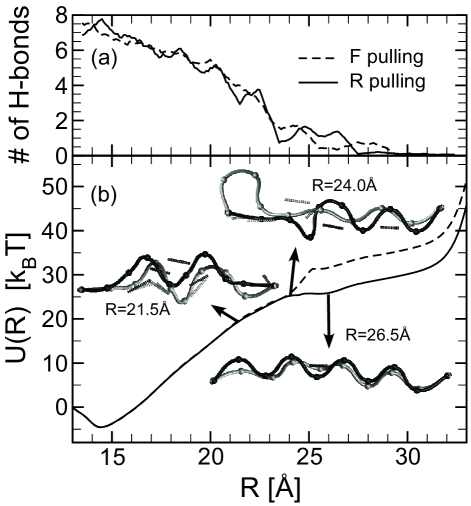
Figure 5: (a) Variation of the number of hydrogen bonds in deca-alanine during the quasi-equilibrium ($v=10^{-4}~{}\text{\AA/ns}$) F and R pullings. (b) The PMF $U(R)$ calculated as the external work done during the quasi-equilibrium F (dashed line) and R (solid line) pullings. The discrepancy between the two PMFs is most likely due to the difference on how the H-bonds are formed and destroyed during the forced folding and unfolding processes, respectively, as indicated in the inset snapshots of the peptide. Dark (lite) color corresponds to the R (F) process.

A careful inspection of these trajectories reveal that the folding and unfolding processes occur through different pathways in the above mentioned range of the RC. Thus, it appears that $R$ is not sufficient to specify the metastable intermediate states of the system, and a more complete description requires the introduction of extra order parameters, e.g., the distribution of the hydrogen bonds (H-bonds) in the peptide. Indeed, the dynamics of the formation and rupture of the H-bonds during folding and unfolding, respectively, may be rather different. As shown in the inset snapshots in Fig. 5b, the formation of the six H-bonds during the R process is much more homogeneous than their rupture during the corresponding F process. This observation is reinforced by the time dependence of the average number of H-bonds in deca-alanine shown in Fig. 5a. Thus there are at least two distinctive pathways in the helix-to-coil transition of deca-alanine, both being explored during quasi-static pullings. During fast pulling, however, one of the pathways is preferred compared to the other.

Finally, as an application of the determined PMF and the diffusion coefficient, which was found to be approximately constant $D\approx 0.27~{}\text{\AA}^{2}/\text{ps}$, we calculated the mean folding time (i.e., coil-to-helix transition) by employing Eq. (13). The theoretical result of $\tau\approx 140$ ps compares rather well with the MFPT of $\approx 100$ ps obtained from the $100$ free MD refolding simulations described in Sec. III.1.

IV K⁺ transport in gramicidin A channel

Gramicidin A (gA) is the smallest known ion channel that selectively conducts cations across lipid bilayers Wallace (1986). gA is a dimer of two barrel-like $\beta$-helices that form a $\sim 26$ Å long and $4-5$ Å wide cylindrical pore through the lipid membrane (Fig. 6). Each helix consists of 15 alternating Asp and Leu amino acids. Due to its structural simplicity, gA is an important testing system for ion permeation models, and it has been extensively studied in the literature both experimentally and through computer modeling.

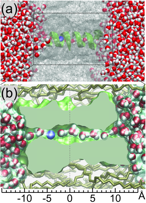
Figure 6: (color online). (a) Gramicidin-A channel ($\beta$-helix dimer colored in green) in POPE lipid bilayer (grey), solvated in water (van der Waals representation). The potassium ions is shown as a blue sphere. (b) Cross-section of the gramicidin A channel. The $K^{+}$ ion (blue) and the water molecules move single file inside the pore. (Created with the program VMD Humphrey et al. (1996a)).

NMR studies have shown that each end of the channel has a cation binding site that is occupied as the ion concentration is increased Tian and Cross (1999) . The conductance is at maximum when the average ion population in the channel is one. The backbone carbonyls inside the pore are oriented such that the electronegative oxygen atoms face inward. The cation selectivity of gA is mainly due to these oxygens, which attract cations and repel anions Jordan (1990); Roux et al. (2000); Kuyucak et al. (2001).

In spite of its structural simplicity, the energetics of the ion transport through gA is far from trivial. Computationally, most of the difficulty arises from the sensitivity to errors due to finite-size effects and from the poor description of the polarization effects by the existing force-fields. Besides the cation gA also accommodates $\sim 6$ single-file water molecules Finkelstein and Andersen (1981) (see Fig. 6b) whose arrangement and orientation seems to play an important role in stabilizing the ion within the channel Allen et al. (2004a).

Previous PMF calculations of the potassium ion, $K^{+}$, through gA yielded a large central barrier that resulted in a conductance orders of magnitude below those measured. In has been speculated that the measured conductance can be reproduced by a PMF that has a $\sim 8$ k_BT deep energy well at both ends of the channel and a $\sim 5$ k_BT barrier in the middle Edwards et al. (2002). Although PMF calculation methods that try to compensate for finite-size and polarization effects have improved in recent years, they continue to yield results that do not match the experimental ones. Most of these methods employ equilibrium MD simulations with umbrella sampling Allen et al. (2006a); Bastug et al. (2006); Allen et al. (2004b) and combined MD simulations with continuum electrostatics theory Mamonov et al. (2003). Recent attempt to apply the JE method (see Sec. II) for calculating the PMF of $K^{+}$ in gA did not yield the desired result Bastug et al. (2008). Here we apply our FR method to calculate both the PMF, $U(z)$, and the position dependent diffusion coefficient, $D(z)$, of $K^{+}$ in gA, and compare our results with the ones from the literature.

IV.1 Computer modeling and SMD simulations

The computer model of gA was constructed from its high resolution NMR structure (Protein Data Bank code 1JNO Townsley et al. (2001)). After adding the missing hydrogens, the structure was energy minimized. Using the VMD Humphrey et al. (1996b) plugin Membrane the system was inserted into a previously pre-equilibrated patch of POPE lipid bilayer with size $72\times 72$ Å². Lipids within $0.55$ Å of the protein were removed. Then, the membrane-protein complex was solvated in water, using the VMD plugin Solvate. The final system contained a total of $36,727$ atoms, including 155 lipid molecules and $5,700$ water molecules. After proper energy minimization and $0.5$ ns long equilibration of the system, a $K^{+}$ ion was added at the entrance of the channel. To preserve change neutrality a $Cl^{-}$ counterion was also added to the solvent. Finally, the system was again energy minimized for $10,000$ steps and equilibrated for $0.5$ ns with $K^{+}$ placed in three different positions along the $z$-axis of the channel, namely at $z\in\{-15,0,15\}$ Å. The origin of the $z$-axis corresponded to the middle of gA (see Fig. 6b). In order to prevent the pore from being dragged during the SMD pulls of the $K^{+}$ ion, two types of restraints were imposed: (i) backbone atoms restrained to their equilibrium positions (referred to as fully restrained); and (ii) backbone atoms restrained only along the $z$-axis (referred to as z-restrained).

The F and R SMD simulations (needed to obtain the PMF using the FR method) were performed on three systems: (S1) backbone of the channel fully restrained with only one pair of $K^{+}$ and $Cl^{-}$ ions in the system; (S2) backbone of the channel fully restrained with $200$ mM electrolyte concentration (obtained by adding $20$ extra pairs of $K^{+}$ and $Cl^{-}$ ions to the solvent using the VMD plugin Autoionize); and (S3) backbone of the channel $z$-restrained and electrolyte concentration $200$ mM. A total of $10$ F and $10$ R SMD pulls were performed along the $z$-axis of gA on two segments: $z\in[-15,0]$ Å and $z\in[0,15]$ Å, corresponding to the two helical monomers. The pulling speed was $v=15$ Å/ns, while the spring constant of the harmonic potential that guided $K^{+}$ across the pore was $k=20$ kcal/mol/Ų.

IV.2 Results and discussion

A comparison of the PMFs of $K^{+}$ along the axis of gA obtained for systems S1, S2 and S3 by employing the FR method is shown in Fig. 7. For gA with fully restrained backbones (i.e., systems S1 and S2) the PMFs have only a weak dependence on the electrolyte concentration, and exhibit a huge central potential barrier of $\sim 40$ k_BT, which is due to the artificially imposed rigidity of the system.

Figure 7: Comparison of PMFs obtained for systems S1 (thin solid line), S2 (dotted line) and S3 for two different pulling protocols: (i) pulling force on $K^{+}$ applied along the $z$-direction (dashed line), and (ii) $K^{+}$ pulled along the axis of the channel (thick solid line).

Once the flexibility of the gA channel in the plane of the membrane is restored by restraining the backbone atoms only along the $z$-axis (i.e., system S3), the central barrier of the PMF decreases to $\sim 15$ k_BT, as shown in Fig. 7 (thick solid line). The transverse flexibility of the channel leads to fluctuations in its radius that facilitate the diffusion of $K^{+}$ along the pore. This is in total agreement with previously published results, which emphasize the crucial role played by the flexibility of the gA channel in its cation transport properties Allen et al. (2004b); Bastug et al. (2006); Corry and Chung (2005). The PMF for system S3 was determined with the FR method by employing two different pulling protocols. First, the pulling force on $K^{+}$ was applied along the $z$-axis (dashed line in Fig. 7) but there was no restrain on the cation’s motion in the cross section of the pore (i.e., in the $xy$-plane). In the second set of pullings, beside the elastic pulling force oriented along the $z$-axis, the potassium ion was constrained to move along the axis of the channel (thick solid line in Fig. 7). As one can see in Fig. 7, both pulling protocols yielded essentially the same PMF. Thus, we preferred using routinely the second pulling method especially because during the first one the potassium ion occasionally escaped between the two helices into the lipid bilayer.

The PMF, $U(z)$, was calculated separately for the two segments (corresponding to the two helical monomers) using Eqs. (9b). The work done during the F and R SMD pullings are plotted in Fig. 8a and Fig. 8b, respectively.

Figure 8: Results of the FR method calculations for system S3 and SMD pulling speed $v=15$ Å/ns. (a) individual (thin lines) and mean (thick line) work for F pulls; (b) individual (thin lines) and mean (thick line) work for R pulls; (c) $U(z)$ along the two segments (dashed line); the symmetrized PMF is shown as solid line (see text); (d) mean dissipative work $\overline{W}_{d}(z)$ along the two segments, $z\in(-15,0)$ Å (dotted line) and $z\in(0,15)$ Å (dashed line), and their arithmetic mean (solid line). The slope of the linear $\overline{W}_{d}(z)$ yields a constant diffusion coefficient $D=10.34$ Å²/ns.

Due to the symmetry of gA with respect to its center, the PMF for the two segments (dashed lines in Fig. 8c) form nearly mirror-images. Therefore, a better estimate of the PMF for the entire gA can be obtained by symmetrizing $U(z)$ with respect to the center of the channel (i.e. $z=0$ Å) (solid line in Fig. 8c). The F and R mean dissipative works, $\overline{W}_{d}^{F/R}(z)$, (averaged over the two segments) are also shown in Fig. 8d (dotted and dashed lines, respectively). The fact that $\overline{W}_{d}^{F}(z)$ and $\overline{W}_{d}^{R}(z)$ closely match each other is another indication that our FR method seems to work fine in the case of the gA channel too. Note that $\overline{W}_{d}(z)$, averaged over the F and R processes, (thick line in Fig. 8d) is almost linear, which according to Eq. (11) yields a constant diffusion coefficient $D\approx 10.3$ Å²/ns. Now, the obtained $D$ and $U(z)$ can be used to solve Eqs. (12a) and/or (12b) for making prediction on the long time dynamics of the $K^{+}$ ion in the gA channel.

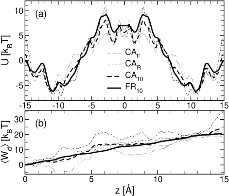
Figure 9: Comparison between the FR method (thick solid lines) and the cumulant approximation of the JE approach (thick dashed lines) for the: (a) potential of mean force and (b) mean dissipative work, obtained from a small number (only $10$) of F and R fast SMD pulling trajectories. The JE method was employed in both F (dotted lines) and R (dash-dotted lines) directions.

The comparison between $U(z)$ and $\overline{W}_{d}(z)$ obtained from the FR method (thick solid lines) and the cumulant approximation (CA) of the JE approach (thick dashed lines), respectively, is shown in Fig. 9a. The bias in the cumulant approximation of the JE method applied either to the F (CA_F, dotted lines) or to the R (CA_R, dash-dotted lines) processes is manifest in Fig. 9. While the former (CA_F) systematically underestimates the peaks in the PMF and the corresponding mean dissipative work, the latter (CA_R) systematically overestimates the same quantities. The difference between the central barrier height of the CA_F and CA_R PMFs is $3.5$ k_BT, while at the channel entrance the difference is almost twice as big ($7$ k_BT). The negative (positive) bias in CA_F (CA_R) is due to the fact that the JE approach uses explicitly the variance (i.e., the 2nd cumulant) of the corresponding non-equilibrium work distributions, which (unlike the mean work) cannot be accurately estimated from a few SMD pullings (see Sec. II). However, by averaging CA_F and CA_R the opposite biases more or less cancel out and the resulting mean PMF (thick dashed line in Fig. 9a) becomes a close match to $U(z)$ calculated from the FR method. According to Fig. 9b, the same conclusion can be drawn for the mean dissipative work as well.

Our $U(z)$, calculated using the FR method, (thick solid line in Fig. 10) has two $\sim 6$ $k_{B}T$ deep wells positioned at the entrances in the channel ($z\approx\pm 10.8$Å) and two high barriers of $\sim 15$ $k_{B}T$ positioned close to the center of the channel ($z\approx\pm 3$ Å). Another small barrier ($\sim 1.4$ $k_{B}T$) appears to be located between the two high barriers, right at the geometrical center of gA. This small center barrier is well separated by the two main ones by a potential well of $\sim 3.5$ k_BT. According to Fig. 10, our PMF (thick solid line) is rather similar to the ones reported in recent publications by Bastug et al Bastug et al. (2006) (double-dot-dashed line) and by Allen et al Allen et al. (2006a) (dot-dashed line). These authors used the standard umbrella sampling (US) method Roux (1995); Kumar et al. (1995) to calculate their PMFs. As shown in Fig. 10, besides the small difference in the positions of the wells at the ends of the gA channel, there are two notable differences between the PMFs obtained by the FR and US methods. First, the barrier height of the PMF computed with the FR method is only $\sim 15$ k_BT as compared to $\sim 20$ k_BT obtained from US. Second, the central peak in $U(z)$ obtained from the FR (US) method is $\sim 2$ k_BT below (above) the two main peaks.

Figure 10: PMFs of $K^{+}$ in the gA channel determined from the FR method (by employing different SMD pulling protocols as described in the text), and the umbrella sampling method Bastug et al. (2006); Allen et al. (2006a).

To test the reliability of the FR method for determining $U(z)$, besides the standard pulling protocol (involving $10$ SMD pulls in both F and R directions with a pulling speed $v=15$ Å/ns), we have used two additional ones, involving only $5$ SMD pulls in both F and R directions. The two pulling protocols differed only in their pulling speeds, namely $v=15$ Å/ns in the first (thin-solid line in Fig. 10) and $v=30$ Å/ns (dotted line in Fig. 10) in the second. As seen in Fig. 10, all three FR method calculations yielded a consistent PMF, with noticeable differences only around the ends of the gA channel.

Although the FR method leads to $U(z)$ similar to the US result (albeit with a smaller main barrier height) none of these PMFs is suitable for reproducing the experimentally measured $K^{+}$ conductivity of the gA channel. This would require a channel entrance well depth of $\sim 8$ k_BT and a main barrier height of $\sim 5$ k_BT Edwards et al. (2002). The main problems in getting these values are due to the limitations of the currently used MD methods that use empirical non-polarizable forcefields and, therefore, cannot account for the induced polarization in the lipid hydrocarbons and, most importantly, for the polarization of water in the course of the MD simulations Allen et al. (2006a, b).

In order to mimic polarization effects caused by the passage of $K^{+}$ through the channel, we reduced the partial charge of the ion from $+e$ to $+0.5e$ in system S3 (see Sec. IV.1), and carried out new SMD F and R pullings for recalculating the PMF through the FR method. The resulting $U(z)$ is shown in Fig. 10 (dashed line). As one can see, in the new PMF the potential wells at the entrance of the channel moved by $2.5$ Å towards the center and their depth increased to $8.5$ $k_{B}T$. Furthermore, in a more dramatic change, the height of the barrier decreased from $\sim 15$ k_BT to $\sim 4.2$ k_BT. Although the above approach to account for polarization effects is rather simplistic, the obtained PMF (apart from the new positions of the potential wells) has the previously estimated form Edwards et al. (2002) that is capable for describing quantitatively the transport of $K^{+}$ in gA.

V Conclusions

In this paper we have shown that the FR method Kosztin et al. (2006) provides an effective approach for calculating both the PMF, $U(R)$, and the diffusion coefficient, $D(R)$, along a properly chosen reaction coordinate $R$, in biomolecular systems by using only a small number of fast forward and time reversed constant velocity SMD simulations. The obtained PMFs for deca-alanine are in good agreement with the ones reported in recent studies Henin and Chipot (2004); Park et al. (2003). We have found that computationally the FR method is more efficient and accurate than similar PMF calculation methods, e.g., the one based on the Jarzynski equality. By employing the computed PMF and diffusion coefficient in a suitable stochastic model we could estimate important characteristics of the studied systems, e.g., the mean folding time of the stretched deca-alanine.

We also applied the FR method to calculate the PMF of a potassium ion through the gramicidin A channel. As expected from previous umbrella sampling calculations, the obtained PMF featured a main central barrier of height $\sim 15$ k_BT and two wells at the entrance in the channel with depth $\sim 6$ $k_{B}T$. The PMF was reproduced rather well when using a smaller number of SMD pulling trajectories and/or higher SMD pulling speeds, confirming the reliability of the FR method. The channel protein flexibility, maintained in the SMD simulations by restraining the corresponding backbone atoms only along the axis of the channel, has been shown to play a major role in the transport of $K^{+}$ in gramicidin A. Indeed, the height of the main potential barrier in a rigid channel is almost three times higher than in the flexible one. The dissipative work inside the channel was found to be linear in $z$, yielding a constant diffusion coefficient $D\approx 10.3$ Å²/ns. The PMF calculated from the same SMD pulls using Jarzynski’s equality with the cumulant approximation yielded inconsistent results for both forward and reverse directions. However, the biases in these to directions almost cancel out when averaging the forward and reverse PMFs, leading to almost the same result as the FR method. Furthermore, the FR method yielded consistently PMFs similar to the ones using the traditional umbrella sampling method but in considerably less time (i.e., $\sim 3$ days per PMF on a 64 CPU, 2.8GHz Intel Xeon EM64T, cluster). However, the conduction of the channel cannot be reproduced with any of the computed PMF profiles, mainly because of the very large central barrier. The main problem in determining PMFs in ion channels through MD simulations is the poor treatment of polarization effects by the current non-polarizable forcefields. To account for the polarization of K⁺ inside the channel, its effective point charge was reduced to $+0.5e$. The recalculated PMF exhibited barrier and well sizes very close to the values needed to reproduce the experimental data. Hopefully, with new polarizable force fields the FR method will provide a simple to use, efficient and reliable tool for calculating PMFs for ion and molecular transport through channel proteins.

References

- Roux (2002) B. Roux, Curr. Opin. Struct. Biol. 12, 182 (2002).
- Becker et al. (2001) O. M. Becker, A. D. MacKerell, B. Roux, and M. Watanabe, eds., Computational Biochemistry and Biophysics (Marcel Dekker, New York, 2001).
- Kosztin et al. (2006) I. Kosztin, B. Barz, and L. Janosi, J. Chem. Phys. 124, 064106 (2006).
- Frenkel and Smit (2002) D. Frenkel and B. Smit, Understanding Molecular Simulation From Algorithms to Applications (Academic Press, California, 2002).
- Roux (1995) B. Roux, Comput. Phys. Commun. 91, 275 (1995).
- Torrie and Valleau (1977) Torrie and Valleau, Journal of Computational Physics 23, 187 (1977).
- Park and Schulten (2004) S. Park and K. Schulten, J. Chem. Phys. 120, 5946 (2004).
- Park et al. (2003) S. Park, F. Khalili-araghi, E. Tajkhorshid, and K. Schulten, J. Chem. Phys. 119, 3559 (2003).
- Isralewitz et al. (2001) B. Isralewitz, J. Baudry, J. Gullingsrud, D. Kosztin, and K. Schulten, J. Mol. Graph. 19, 13 (2001).
- Jensen et al. (2002) M. O. Jensen, S. Park, E. Tajkhorshid, and K. Schulten, Proc. Natl. Acad. Sci. U. S. A. 99, 6731 (2002).
- Crooks (2000) G. E. Crooks, Phys. Rev. E 61, 2361 (2000).
- Hummer and Szabo (2001) G. Hummer and A. Szabo, Proc. Natl. Acad. Sci. U. S. A. 98, 3658 (2001).
- Shirts et al. (2003) M. R. Shirts, E. Bair, G. Hooker, and V. S. Pande, Phys. Rev. Lett. 91, 140601 (2003).
- Zwanzig (2001) R. Zwanzig, Nonequilibrium statistical mechanics (Oxford University Press, Oxford ; New York, 2001), 00023880 Robert Zwanzig. Includes bibliographical references (p. 211) and index.
- Risken (1996) H. Risken, The Fokker-Planck Equation: Methods of Solution and Applications (Springer-Verlag Telos, 1996), 3rd ed.
- Henin and Chipot (2004) J. Henin and C. Chipot, J. Chem. Phys. 121, 2904 (2004).
- Procacci et al. (2006) P. Procacci, S. Marsili, A. Barducci, G. F. Signorini, and R. Chelli, J Chem Phys 125, 164101 (2006).
- Humphrey et al. (1996a) W. Humphrey, A. Dalke, and K. Schulten, Jour. Mol. Graph. 14, 33 (1996a).
- Phillips et al. (2005) J. C. Phillips, R. Braun, W. Wang, J. Gumbart, E. Tajkhorshid, E. Villa, C. Chipot, R. D. Skeel, L. Kale, and K. Schulten, J. Comput. Chem. 26, 1781 (2005).
- MacKerell Jr. et al. (1992) A. D. MacKerell Jr., D. Bashford, M. Bellott, et al., FASEB J. 6, A143 (1992).
- MacKerell Jr. et al. (1998) A. D. MacKerell Jr., D. Bashford, M. Bellott, et al., J. Phys. Chem. B 102, 3586 (1998).
- Miyamoto and Kollman (1992) S. Miyamoto and P. A. Kollman, J. Comp. Chem. 13, 952 (1992).
- Wallace (1986) B. A. Wallace, Biophys. J. 49, 295 (1986).
- Tian and Cross (1999) F. Tian and T. A. Cross, J. Mol. Biol. 285, 1993 (1999).
- Jordan (1990) P. C. Jordan, Biophys. J. 58, 1133 (1990).
- Roux et al. (2000) B. Roux, S. Berneche, and W. Im, Biochemistry 39, 13295 (2000).
- Kuyucak et al. (2001) S. Kuyucak, O. S. Andersen, and S. H. Chung, Rep. Prog. Phys. 64, 1427 (2001).
- Finkelstein and Andersen (1981) A. Finkelstein and O. S. Andersen, J. Membr. Biol. 59, 155 (1981).
- Allen et al. (2004a) T. W. Allen, O. S. Andersen, and B. Roux, Proc. Natl. Acad. Sci. U.S.A. 101, 117 (2004a).
- Edwards et al. (2002) S. Edwards, B. Corry, S. Kuyucak, and S. H. Chung, Biophys. J. 83, 1348 (2002).
- Allen et al. (2006a) T. W. Allen, O. S. Andersen, and B. Roux, Biophys. J. 90, 3447 (2006a).
- Bastug et al. (2006) T. Bastug, A. Gray-Weale, S. M. Patra, and K. S., Biophys. J. 90, 2285 (2006).
- Allen et al. (2004b) T. W. Allen, O. S. Andersen, and B. Roux, J. Gen. Physiol. 124, 679 (2004b).
- Mamonov et al. (2003) A. B. Mamonov, R. D. Coalson, A. Nitzan, and M. G. Kurnikova, Biophys. J. 84, 3646 (2003).
- Bastug et al. (2008) T. Bastug, P.-C. Chen, S. M. Patra, and S. Kuyucak, J. Chem. Phys. 128, 155104 (2008).
- Townsley et al. (2001) L. E. Townsley, W. A. Tucker, S. Sham, and J. F. Hinton, Biochemistry 40, 11676 (2001).
- Humphrey et al. (1996b) W. Humphrey, A. Dalke, and K. Schulten, J. Mol. Graphics 14, 33 (1996b).
- Corry and Chung (2005) B. Corry and S. H. Chung, Eur. Biophys. J. 34, 208 (2005).
- Kumar et al. (1995) S. Kumar, J. M. Rosenberg, D. Bouzida, R. H. Swendsen, and P. A. Kollman, J. Comput. Chem. 16, 1339 (1995).
- Allen et al. (2006b) T. W. Allen, O. S. Andersen, and B. Roux, Biophys. Chem. 124, 251 (2006b).