Probabilistic theories:
what is special about Quantum Mechanics?

Abstract.

Quantum Mechanics (QM) is a very special probabilistic theory, yet we don’t know which operational principles make it so. All axiomatization attempts suffer at least one postulate of a mathematical nature. Here I will analyze the possibility of deriving QM as the mathematical representation of a fair operational framework, i.e. a set of rules which allows the experimenter to make predictions on future events on the basis of suitable tests, e.g. without interference from uncontrollable sources. Two postulates need to be satisfied by any fair operational framework: NSF: no-signaling from the future—for the possibility of making predictions on the basis of past tests; PFAITH: existence of a preparationally faithful state—for the possibility of preparing any state and calibrating any test. I will show that all theories satisfying NSF admit a C^∗-algebra representation of events as linear transformations of effects. Based on a very general notion of dynamical independence, it is easy to see that all such probabilistic theories are non-signaling without interaction (non-signaling for short)—another requirement for a fair operational framework. Postulate PFAITH then implies the local observability principle, the tensor-product structure for the linear spaces of states and effects, the impossibility of bit commitment and additional features, such an operational definition of transpose, a scalar product for effects, weak-selfduality of the theory, and more. Dual to Postulate PFAITH an analogous postulate for effects would give additional quantum features, such as teleportation. However, all possible consequences of these postulates still need to be investigated, and it is not clear yet if we can derive QM from the present postulates only.

What is special about QM is that also effects make a C^∗-algebra. More precisely, this is true for all hybrid quantum-classical theories, corresponding to QM plus super-selection rules. However, whereas the sum of effects can be operationally defined, the notion of effect abhors any kind of composition. Based on the natural postulate of atomicity of evolution (AE) one can define composition of effects by identifying them with atomic events through the Choi-Jamiolkowski isomorphism (CJ). In this way the quantum-classical hybrid is selected within the large arena of non-signaling probabilistic theories, including the Popescu-Rohrlich boxes. The CJ isomorphism looks natural in an operational context, and it is hoped that it will soon be converted into an operational principle.

• To my friend and mentor, Professor Attilio Rigamonti.

• Unperformed experiments have no results.

• —Asher Peres

1. Introduction

After more than a century from its birth, Quantum Mechanics (QM) remains mysterious. We still don’t have general principles from which to derive its remarkable mathematical framework, as it happened for the amazing Lorentz’s transformations, lately re-derived by Einstein’s from invariance of physical laws on inertial frames and from constancy of the speed of light.

Despite the utmost relevance of the problem of deriving QM from operational principles, research efforts in this direction have been sporadic. The deepest of the early attacks on the problem were the works of Birkoff, von Neumann, Jordan, and Wigner, attempting to derive QM from a set of axioms with as much physical significance as possible [1, 2]. The general idea in Ref. [1] is to regard QM as a new kind of prepositional calculus, a proposal that spawned the research line of quantum logic, based on von Neumann’s observation that the two-valued observables—represented in his formulation of QM by orthogonal projection operators—constitute a kind of “logic” of experimental propositions. After a hiatus of two decades of neglect, interest in quantum logic was revived by Varadarajan [3], and most notably by Mackey [4], who axiomatized QM within an operational framework, with the single exception of an admittedly ad hoc postulate, which represents the propositional-calculus mathematically in form of an orthomodular lattice. The most significant extension of Mackey’s work is the general representation theorem of Piron [5].

In the early work [2], Jordan, von Neumann, and Wigner considered the possibility of a commutative algebra of observables, with a product which needs only to define squares and sums of observables—the so-called Jordan product of observables $a$ and $b$: $a\circ b:=(a+b)^{2}-a^{2}-b^{2}$. However, such a product is generally non-associative and non-distributive with respect to the sum, and the quantum formalism follows only with additional axioms with no clear physical significance—e.g. a distributivity axiom for the Jordan product. Segal [6] later constructed an (almost) fully operational framework (with no experimental definition of the sum of observables) which allows generally non-distributive algebras of observables, but with a resulting mathematical framework largely more general than QM. As a result of this line of investigation, the purely algebraic formulation of QM gathered popularity versus the original Hilbert-space axiomatization.

In the algebraic axiomatization of QM, a physical system is defined by its $C^{*}$-algebra of observables (with identity), and the states of the system are identified with normalized positive linear functionals over the algebra, corresponding to the probability rules of measurements of observables. Indeed, the $C^{*}$-algebra of observables is more general than QM, since it includes Classical Mechanics as a special case, and generally describes any quantum-classical hybrid, equivalent to QM with super-selection rules. Since in practice two observables are not distinguishable if they always exhibit the same probability distributions, at the operational level one can always take the set of states as observable-separating—in the sense that there are no different observables having the same probability distribution for all states. Conversely the set of observables is state-separating, i.e. there are no different states corresponding to the same probability distribution for all observables. Notice that, in principle, there exist different observables with the same expectation for all states, but higher moments will be different.

The algebra of observables is generally considered to be more “operational” than the usual Hilbert-space axiomatization, however, little is gained more than a representation-independent mathematical framework. Indeed, the algebraic framework is unable to provide operational rules for how to measure sums and products of non-commuting observables. The sum of two observables cannot be given an operational meaning, since a procedure involving the measurements of the two addenda would unavoidably assume that their respective measurements are jointly executable on the same system—i.e. the observables are compatible. The same reasoning holds for the product of two observables. A sum-observable defined as the one having expectation equal to the sum of expectations for all states [7] is clearly not unique, due to the existence of observables having the same expectation for all states, but with different higher moments. The only well defined procedures are those involving single observables, such as the measurement of a function of a single observable, which operationally consists in just taking the function of the outcome.

The Jordan symmetric product has been regarded as a great advance in view of an operational axiomatization, since, in addition to being Hermitian (observables are Hermitian), is defined only in terms of squares and sums of observables—i.e. without products. The definition of $a\circ b$, however, still relies on the notion of sum of observables, which has no operational meaning. Remarkably, Alfsen and Shultz [8, 9] succeeded in deriving the Jordan product from solely geometrical properties of the convex set of states—e.g. orientability and faces shaped as Euclidean balls—however, again with no operational meaning. The problem with the Jordan product is that, in addition to not necessarily being associative, it is not even distributive, as the reader can easily check himself. It turns out that, modulo a few topological assumptions, the Jordan algebras can be embedded in the algebra ${\sf Lin(H)}$ of operators over the Hilbert space ${\sf H}$, whereby $a\circ b=ab+ba$. Such assumptions, however, are still not operational. For further critical overview of these earlier attempts to an operational axiomatization of QM, the reader is also directed to the recent books of Strocchi [7] and Thirring [10].

After a long suspension of research on the axiomatic approach—notably interrupted by the work of Ludwig and his school [11]—in the last years the new field of Quantum Information has renewed the interest on the problem of operational axiomatization of QM, boosted by the new experience on multipartite systems and entanglement. In his seminal paper [12] Hardy derived QM from five “reasonable axioms”, which, more than being truly operational, are motivated on the basis of simplicity and continuity criteria, with the assumption of a finite number of perfectly discriminable states. His axiom 4, however, is still purely mathematical, and is directly related to the tensor product rule for composite systems. In another popular paper [13], Clifton, Bub, and Halvorson have shown how three fundamental information-theoretic constraints—(a) the no-signaling, (b) the no-broadcasting, (c) the impossibility of unconditionally secure bit commitment—suffice to entail that the observables and state space of a physical theory are quantum-mechanical. Unfortunately, the authors already started from a C^∗-algebraic framework for observables, which, as already discussed, has little operational basis, and already coincides with the quantum-classical hybrid. Therefore, more than deriving QM, their informational principles just force the C^∗-algebra of observables to be non-Abelian.

In Ref. [14] I showed how it is possible to derive the formulation of QM in terms of observables represented as Hermitian operators over Hilbert spaces with the right dimensions for the tensor product, starting from few operational axioms. However, it is not clear yet if such framework is sufficient to identify QM (or the quantum-classical hybrid) as the only probabilistic theory resulting from axioms. Later, in Refs. [17, 18, 19] I have shown how a C^∗-algebraic framework for transformations (not for observables!) naturally follows from an operational probabilistic framework.

A very recent and promising direction for attacking the problem of QM axiomatization consists in positioning QM within the landscape of general probabilistic theories, including theories with non-local correlations stronger than the quantum ones, e.g. for the Popescu-Rohrlich boxes (PR-boxes) [20]. Such theories have correlations that are “stronger” than the quantum ones—in the sense that they violate the quantum Cirel’son bound [21]—although they are still non-signaling, thus revealing the fortuitousness of the peaceful coexistence of QM and Special Relativity, in contrast with the claimed implication of QM linearity from the no-signaling condition [22]. Within the framework of the PR-boxes general versions of the no-cloning and no-broadcasting theorems have been proved [23]. In Ref. [24] it has been shown that certain features generally thought of as specifically quantum, are indeed present in all except classical theories. These include the non-unique decomposition of a mixed state into pure states, disturbance on measurement (related to the possibility of secure key distribution), and no-cloning. More recently, necessary and sufficient conditions have been established for teleportation [25], i.e. for reconstructing the state of a system on a remote identical system, using only local operations and joint states. In all these works Quantum Information has inspired task-oriented axioms to be considered in a general operational framework that can incorporate QM, classical theory, and other non-signaling probabilistic theories (for an illustration of this general point of view see also Ref. [26]).

In the present paper I will consider the possibility of deriving QM as the mathematical representation of a fair operational framework, i.e. a set of rules which allows the experimenter to make predictions regarding future events on the basis of suitable tests, in a spirit close to Ludwig’s axiomatization [11]. States are simply the compendia of probabilities for all possible outcomes of any test. I will consider a very general class of probabilistic theories, and examine the consequences of two Postulates that need to be satisfied by any fair operational framework:

• no-signaling from the future, implying that it is possible to make predictions based on present tests;

• existence of preparationally faithful states, implying the possibility of preparing any state and calibrating any test.

NSF is implicit in the definition itself of conditional probabilities for cascade-tests, entailing that events are identified with transformations, whence evolution is identified with conditioning. As we will see, such identifications lead to the notion of effect of Ludwig, i.e. the equivalence class of events occurring with the same probability for all states. I will show how we can introduce operationally a linear-space structure for effects. I will then show how all theories satisfying NSF admit a C^∗-algebra representation of events as linear transformations of effects.

Based on a very general notion of dynamical independence, entailing the definition of marginal state, it is immediately seen that all these theories are non-signaling, which is the current way of saying that the theories satisfy the principle of Einstein locality, namely that there can be no detectable effect on a system due to anything done to another non-interacting system. This is clearly another requirement for a fair operational framework. Postulate PFAITH then implies the local observability principle, namely the possibility of achieving an informationally complete test using only local tests—another requirement for a fair operational framework. The same postulate also implies many other features that are typically quantum, such as the tensor-product structure for the linear spaces of states and effects, the isomorphism of cones of states and effects—a weaker version of the quantum selfduality—impossibility of bit commitment (which in Ref. [13] we remind it was used as a postulate itself to derive QM), and many more. Dual to Postulate PFAITH an analogous postulate for effects would give additional quantum features, such as teleportation. However, all possible consequences of these postulates still need to be investigated, and it is not clear yet if one can derive QM from these principles only.

In order to provide a route for seeking new candidates for operational postulates one can short-circuit the axiomatic framework to select QM using a mathematical postulate dictated by what is really special about the quantum theory, namely that not only transformations, but also effects form a C^∗-algebra (more precisely, this is true for all hybrid quantum-classical theories, i.e. corresponding to QM plus super-selection rules). However, whereas the sum of effects can be operationally defined, their composition has no operational meaning, since the notion itself of “effect” abhors any kind of composition. I will then show that with another natural postulate,

• atomicity of evolution,

along with the mathematical postulate,

• Choi-Jamiolkowski isomorphism [27, 28],

it is possible to identify effects with “atomic” events, i.e. elementary events which cannot be refined as the union of events. Via the composition of atomic events we can then define the composition of effects, thus selecting the quantum-classical hybrid among all possible general probabilistic theories (including the PR-boxes, which indeed satisfy both NSF and PFAITH).

The CJ isomorphism looks natural in an operational context, and it is hoped that it will be converted soon into an operational postulate.

The present operational axiomatization will adhere to the following three general principles:

1. (Strong Copenhagen) Everything is defined operationally, including all mathematical objects. Operationally indistinguishable entities are identified.

2. (Mathematical closure) Mathematical completion is taken for convenience.

3. (Operational closure) Every operational option that is implicit in the formulation is incorporated in the axiomatic framework.

An example of the application of the Strongly Copenhagen principle is the notion of system, which here I will identify with a collection of tests—the tests that can be performed over the system. A typical case of operational identification is that of events occurring with the same probability and producing the same conditioning. Another case is the statement that the set of states is separating for effects and viceversa. Examples of mathematical closure are the norm closure, the algebraic closure, and the linear span. It is unquestionable that these are always idealizations of operational limiting cases, or they are introduced just to simplify the mathematical formulation (e.g. real numbers versus the “operational” rational numbers). Operational completeness, on the other hand, does not affect the corresponding mathematical representation, since every incorporated option is already implicit in the formulation. This is the case, for example, for convex closure, closure under coarse-graining, etc. which are already implicit in the probabilistic formulation.

2. C^∗-algebra representation of probabilistic theories

2.1. Tests and states

A probabilistic operational framework is a collection of tests $\mathbb{A},\mathbb{B},\mathbb{C},\ldots$ each being a complete collection $\mathbb{A}=\{\mathscr{A}_{i}\}$, $\mathbb{B}=\{\mathscr{B}_{j}\}$, $\mathbb{C}=\{\mathscr{C}_{k}\}$, …of mutually exclusive events $\mathscr{A}_{i},\mathscr{B}_{j},\mathscr{C}_{k},\ldots$ occurring probabilistically; events that are mutually exclusive are often called outcomes. The same event can occur in different tests, with occurrence probability independent on the test. A singleton test—also called a channel—$\mathbb{D}=\{\mathscr{D}\}$ is deterministic: it represents a non-test, i.e. a free evolution. The union $\mathscr{A}\cup\mathscr{B}$ of two events corresponds to the event in which either $\mathscr{A}$ or $\mathscr{B}$ occurred, but it is unknown which one. A refinement of an event $\mathscr{A}$ is a set of events $\{\mathscr{A}_{i}\}$ occurring in some test such that $\mathscr{A}=\cup_{i}\mathscr{A}_{i}$. The experiment itself $\mathbb{A}$ can be regarded as the deterministic event corresponding to the complete union of its outcomes, and when regarded as an event it will be denoted by the different notation $\mathscr{D}_{\mathbb{A}}$. The opposite event of $\mathscr{A}$ in $\mathbb{A}$ will be denoted as $\overline{\mathscr{A}}:=\complement_{\mathbb{A}}\mathscr{A}$. The union of events transforms a test $\mathbb{A}$ into a new test $\mathbb{A}^{\prime}$ which is a coarse-graining of $\mathbb{A}$, e.g. $\mathbb{A}=\{\mathscr{A}_{1},\mathscr{A}_{2},\mathscr{A}_{3}\}$ and $\mathbb{A}^{\prime}=\{\mathscr{A}_{1},\mathscr{A}_{2}\cup\mathscr{A}_{3}\}$. Vice-versa, we will call $\mathbb{A}$ a refinement of $\mathbb{A}^{\prime}$.

The state $\omega$ describing the preparation of the system is the probability rule $\omega(\mathscr{A})$ for any event $\mathscr{A}\in\mathbb{A}$ occurring in any possible test $\mathbb{A}$. For each test $\mathbb{A}$ we have the completeness $\sum_{\mathscr{A}_{j}\in\mathbb{A}}\omega(\mathscr{A}_{j})=1$. States themselves are considered as special tests: the state-preparations.

2.2. Cascading, conditioning, and transformations

The cascade $\mathbb{B}\circ\mathbb{A}$ of two tests $\mathbb{A}=\{\mathscr{A}_{i}\}$ and $\mathbb{B}=\{\mathscr{B}_{j}\}$ is the new test with events $\mathbb{B}\circ\mathbb{A}=\{\mathscr{B}_{j}\circ\mathscr{A}_{i}\}$, where $\mathscr{B}\circ\mathscr{A}$ denotes the composite event $\mathscr{A}$ “followed by” $\mathscr{B}$ satisfying the following

Postulate NSF (No-signaling from the future). The marginal probability $\sum_{\mathscr{B}_{j}\in\mathbb{B}}\omega(\mathscr{B}_{j}\circ\mathscr{A})$ of any event $\mathscr{A}$ is independent on test $\mathbb{B}$, and is equal to the probability with no test $\mathbb{B}$, namely

(1) $$\sum_{\mathscr{B}_{j}\in\mathbb{B}}\omega(\mathscr{B}_{j}\circ\mathscr{A})=:f(\mathbb{B},\mathscr{A})\equiv\omega(\mathscr{A}),\quad\forall\mathbb{B},\,\mathscr{A},\,\omega.$$

NSF is part of the definition itself of test-cascade, however, we treat it as a separate postulate, since it corresponds to the choice of the arrow of time. The interpretation of the test-cascade $\mathbb{B}\circ\mathbb{A}$ is that “test $\mathbb{A}$ can influence test $\mathbb{B}$ but not vice-versa.” Postulate NSF allows one to define the conditioned probability $p(\mathscr{B}|\mathscr{A})=\omega(\mathscr{B}\circ\mathscr{A})/\omega(\mathscr{A})$ of event $\mathscr{B}$ occurring conditionally on the previous occurrence of event $\mathscr{A}$. It also guarantees that the probability of $\mathscr{B}$ remains independent of the test $\mathbb{B}$ when conditioned.

Conditioning sets a new probability rule corresponding to the notion of conditional state $\omega_{\mathscr{A}}$, which gives the probability that an event occurs knowing that event $\mathscr{A}$ has occurred with the system prepared in the state $\omega$, namely $\omega_{\mathscr{A}}\doteq\omega(\cdot\circ\mathscr{A})/\omega(\mathscr{A})$. We can now regard the event $\mathscr{A}$ as transforming with probability $\omega(\mathscr{A})$ the state $\omega$ to the (unnormalized) state $\mathscr{A}\omega$ given by

(2) $$\mathscr{A}\omega:=\omega(\cdot\circ\mathscr{A}).$$

Therefore, the notion of cascade and Postulate NSF entail the identification:

event$\equiv$transformation,

which in turn implies the equivalence:

evolution$\equiv$state-conditioning.

Notice that operationally a transformation $\mathscr{A}$ is completely specified by all the joint probabilities in which it is involved, whence, it is univocally given by the probability rule $\mathscr{A}\omega=\omega(\cdot\circ\mathscr{A})$ for all states $\omega$. This is equivalent to specify both the conditional state $\omega_{\mathscr{A}}$ and the probability $\omega(\mathscr{A})$ for all possible states $\omega$, due to the identity

(3) $$\mathscr{A}\omega=\omega(\mathscr{A})\omega_{\mathscr{A}}.$$

In particular the identity transformation $\mathscr{I}$ is completely specified by the rule $\mathscr{I}\omega=\omega$ for all states $\omega$.

2.3. System

In a pure Copenhagen spirit we will identify a system ${\sf S}$ with a collection of tests ${\sf S}=\{\mathbb{A},\mathbb{B},\mathbb{C},\ldots\}$, the collection being operationally closed under coarse-graining, convex combination, conditioning, and cascading, and will includes all states as special tests. Closure under cascading is equivalent to consider mono-systemic evolution, i.e. in which there are only tests for which the output system is the same of the input one. The operator has always the option of performing repeated tests, along with (randomly) alternating tests—say $\mathbb{A}$ and $\mathbb{B}$—in different proportions—say $p$ and $1-p$ ($0<p<1$)—thus achieving the test $\mathbb{C}_{p}=p\mathbb{A}+(1-p)\mathbb{B}$ which is the convex combination of tests $\mathbb{A}$ and $\mathbb{B}$, and is given by $\mathbb{C}_{p}=\{p\mathscr{A}_{1},p\mathscr{A}_{2},\ldots,(1-p)\mathscr{B}_{1},(1-p)\mathscr{B}_{2},\ldots\}$, where $p\mathscr{A}$ is the same event as $\mathscr{A}$, but occurring with a probability rescaled by $p$. Since we will consider always the closure under all operator’s options (this is our operational closure), we will take the system also to be closed under such convex combination. In particular, the set of all states of the system is closed under convex combinations and under conditioning, and we will denote by ${\mathfrak{S}}({\sf S})$ (${\mathfrak{S}}$ for short) the convex set of all possible states of system ${\sf S}$. We will often use the colloquialism “for all possible states $\omega$” meaning $\forall\omega\in{\mathfrak{S}}({\sf S})$, and we will do similarly for other operational objects.

In the following we will denote the set of all possible transformations/events by ${\mathfrak{T}}({\sf S})$, ${\mathfrak{T}}$ for short. The convex structure of ${\sf S}$ entails a convex structure for ${\mathfrak{T}}$, whereas the cascade of tests entails the composition of transformations. The latter, along with the existence of the identity transformation $\mathscr{I}$, gives to ${\mathfrak{T}}$ the structure of convex monoid.

2.4. Effects

From the notion of conditional state two complementary types of equivalences for transformations follow: the conditional and the probabilistic equivalence. The transformations $\mathscr{A}_{1}$ and $\mathscr{A}_{2}$ are conditioning-equivalent when $\omega_{\mathscr{A}_{1}}=\omega_{\mathscr{A}_{2}}$ $\forall\omega\in{\mathfrak{S}}$, namely when they produce the same conditional state for all prior states $\omega$. On the other hand, the transformations $\mathscr{A}_{1}$ and $\mathscr{A}_{2}$ are probabilistically equivalent when $\omega(\mathscr{A}_{1})=\omega(\mathscr{A}_{2})$ $\forall\omega\in{\mathfrak{S}}$, namely when they occur with the same probability. Since operationally a transformation $\mathscr{A}$ is completely specified by the probability rule $\mathscr{A}\omega$ for all states, it follows that two transformations $\mathscr{A}_{1}$ and $\mathscr{A}_{2}$ are fully equivalent (i.e. operationally indistinguishable) when $\mathscr{A}_{1}\omega=\mathscr{A}_{2}\omega$ for all states $\omega$. We will identify two equivalent transformations, and denote the equivalence simply as $\mathscr{A}_{1}=\mathscr{A}_{2}$. From identity (3) it follows that two transformations are equivalent if and only if they are both conditioning and probabilistically equivalent.

A probabilistic equivalence class of transformations defines an effect. In the following we will denote effects with lowercase letters $a,b,c,\ldots$ and denote by $[\mathscr{A}]_{\rm eff}$ the effect containing transformation $\mathscr{A}$. We will also write $\mathscr{A}\in a$ meaning that “the transformation $\mathscr{A}$ belongs to the equivalence class $a$”, or “$\mathscr{A}$ has effect $a$”, and write “$\mathscr{A}\in[\mathscr{B}]_{\rm eff}$ to say that “$\mathscr{A}$ is probabilistically equivalent to $\mathscr{B}$”. Since by definition $\omega(\mathscr{A})=\omega([\mathscr{A}]_{\rm eff})$, hereafter we will legitimately write the variable of the state as an effect, e.g. $\omega(a)$. The deterministic effect will be denoted by $e$, corresponding to $\omega(e)=1$ for all states $\omega$. We will denote the set of effects for a system ${\sf S}$ as ${\mathfrak{E}}({\sf S})$, or just ${\mathfrak{E}}$ for short. The set of effects inherits a convex structure from that of transformations.

By the same definition of state—as probability rule for transformations—states are separated by effects (whence also by transformations), and, conversely, effects are separated by states. Transformations are separated by states in the sense that $\mathscr{A}\neq\mathscr{B}$ iff $\mathscr{A}\omega\neq\mathscr{B}\omega$ for some state. As a consequence, it may happen that the introduction of a new state via some new preparation (such as introducing additional systems) will separate two previously indiscriminable transformations, in which case we will include the new state (and all convex combination with it) in ${\mathfrak{S}}({\sf S})$, and we will complete the system ${\sf S}$ accordingly. We will end with ${\mathfrak{S}}({\sf S})$ separating ${\mathfrak{T}}({\sf S})$ and ${\mathfrak{E}}({\sf S})$, and ${\mathfrak{E}}({\sf S})$ separating ${\mathfrak{S}}({\sf S})$.

The identity $\omega_{\mathscr{A}}(\mathscr{B})\equiv\omega_{\mathscr{A}}([\mathscr{B}]_{\rm eff})$ implies that $\omega(\mathscr{B}\circ\mathscr{A})=\omega([\mathscr{B}]_{\rm eff}\circ\mathscr{A})$ for all states $\omega$, leading to the chaining rule $[\mathscr{B}]_{\rm eff}\circ\mathscr{A}=[\mathscr{B}\circ\mathscr{A}]_{\rm eff}$, corresponding to the “Heisenberg picture” evolution in terms of transformations acting on effects. Notice that transformations act on effects from the right, inheriting the composition rule of transformations ($\mathscr{B}\circ\mathscr{A}$ means ”$\mathscr{A}\text{ followed by }\mathscr{B}$”). Notice also that $e\circ\mathscr{A}\in[\mathscr{I}\circ\mathscr{A}]_{\rm eff}=a$. It follows that for $\mathscr{D}$ deterministic one has $\mathscr{D}\in e$, whence $\mathscr{D}\circ\mathscr{A}\in[\mathscr{A}]_{\rm eff}$.

Consistently, in the “Schrödinger picture”, we have $\mathscr{B}\omega(\cdot\circ\mathscr{A})=\omega(\cdot\circ\mathscr{B}\circ\mathscr{A})$, corresponding to $(\mathscr{B}\circ\mathscr{A})\omega=\omega(\cdot\circ\mathscr{B}\circ\mathscr{A})$. Also, we will use the unambiguous notation $\mathscr{B}\omega(a)=[\mathscr{B}\omega](a)$, whence $\mathscr{B}\omega(a)=\omega(a\circ\mathscr{B})$, and $\omega(a)=\mathscr{A}\omega(e),\;\forall\mathscr{A}\in a$.

2.5. Linear structures for transformations and effects

Transformations $\mathscr{A}_{1}$ and $\mathscr{A}_{2}$, for which one has the bound $\omega(\mathscr{A}_{1})+\omega(\mathscr{A}_{2})\leqslant 1,\;\forall\omega\in{\mathfrak{S}}$ can in principle occur in the same test, and we will call them test-compatible. For test-compatible transformations one can define their addition $\mathscr{A}_{1}+\mathscr{A}_{2}$ via the probability rule

(4) $$(\mathscr{A}_{1}+\mathscr{A}_{2})\omega=\mathscr{A}_{1}\omega+\mathscr{A}_{2}\omega,$$

were we remind that $\mathscr{A}\omega:=\omega(\cdot\circ\mathscr{A})$. Therefore the sum of two test-compatible transformations is just the union-event $\mathscr{A}_{1}+\mathscr{A}_{2}=\mathscr{A}_{1}\cup\mathscr{A}_{2}$, with the two transformations regarded as belonging to the same test. For any test $\mathbb{A}$ we can define its total coarse-graining as the deterministic transformation $\mathscr{D}_{\mathbb{A}}=\sum_{\mathscr{A}_{i}\in\mathbb{A}}\mathscr{A}_{i}$. We can trivially extend the addition rule (4) to any set of (generally non test-compatible) transformations, and to subtraction of transformations as well. Notice that the composition “$\circ$” is distributive with respect to addition “$+$”.

We can define the multiplication $\lambda\mathscr{A}$ of a transformation $\mathscr{A}$ by a scalar $0\leqslant\lambda\leqslant 1$ by the rule

(5) $$\omega(\cdot\circ\lambda\mathscr{A})=\lambda\omega(\cdot\circ\mathscr{A}),$$

namely $\lambda\mathscr{A}$ is the transformation conditioning-equivalent to $\mathscr{A}$, but occurring with rescaled probability $\omega(\lambda\mathscr{A})=\lambda\omega(\mathscr{A})$—as happens in the convex combination of tests. It follows that for every couple of transformations $\mathscr{A}$ and $\mathscr{B}$ the transformations $\lambda\mathscr{A}$ and $(1-\lambda)\mathscr{B}$ are test-compatible for $0\leqslant\lambda\leqslant 1$, consistently with the convex closure of the system ${\sf S}$. By extending the definition (5) to any positive $\lambda$, we then introduce the cone ${\mathfrak{T}}_{+}$ of transformations. We will call an event $\mathscr{A}$ atomic if it has no nontrivial refinement in any test, namely if it cannot be written as $\mathscr{A}=\sum_{i}\mathscr{A}_{i}$ with $\mathscr{A}_{i}\neq\lambda_{i}\mathscr{A}$ for some $i$ and $0<\lambda_{i}<1$. Notice that the identity transformation is not necessarily atomic. The set of extremal rays of the cone ${\mathfrak{T}}_{+}$—denoted by ${\sf Erays}({\mathfrak{T}}_{+})$—contains the atomic transformations.

The notions of i) test-compatibility, ii) sum, and iii) multiplication by a scalar, are naturally inherited from transformations to effects via probabilistic equivalence, and then to states via duality. Correspondingly, we introduce the cone of effects ${\mathfrak{E}}_{+}$, and, by duality, we extend the cone of states ${\mathfrak{S}}_{+}$ to the dual cone of ${\mathfrak{E}}_{+}$, completing the set of states ${\mathfrak{S}}$ to the cone-base of ${\mathfrak{S}}_{+}$ made of all positive linear functionals over ${\mathfrak{E}}_{+}$ normalized at the deterministic effect, namely all in-principle legitimate states (in parallel we complete the system ${\sf S}$ with the corresponding state-preparations). We call such a completion of the set of states the no-restriction hypothesis for states, corresponding to the state–effect duality, namely the convex cones of states ${\mathfrak{S}}_{+}$ and of effects ${\mathfrak{E}}_{+}$ are dual each other. The state cone ${\mathfrak{S}}_{+}$ introduce a natural partial ordering $\geqslant$ over states and over effect (via duality), and one has $a\in{\mathfrak{E}}$ iff $0\leqslant a\leqslant e$. Thus the convex set ${\mathfrak{E}}$ is a truncation of the cone ${\mathfrak{E}}_{+}$, whereas ${\mathfrak{S}}$ is a base for the cone ${\mathfrak{S}}_{+}$ defined by the normalization condition $\omega\in{\mathfrak{S}}$ iff $\omega\in{\mathfrak{S}}_{+}$ and $\omega(e)=1$. In the following it will be useful also to express the probability rule $\omega(a)$ also in its dual form $a(\omega)=\omega(a)$, with the effect acting on the state as a linear functional.

By extending to any real (complex) scalar $\lambda$ Eq. (5) we build the linear real (complex) span ${\mathfrak{T}}_{\mathbb{R}}={\sf Span}_{\mathbb{R}}({\mathfrak{T}})$ (${\mathfrak{T}}_{\mathbb{C}}={\sf Span}_{\mathbb{C}}({\mathfrak{T}})$). The Cartesian decomposition ${\mathfrak{T}}_{\mathbb{C}}={\mathfrak{T}}_{\mathbb{R}}\oplus i{\mathfrak{T}}_{\mathbb{R}}$ holds, i.e. each element $\mathscr{A}\in{\mathfrak{T}}_{\mathbb{C}}$ can be uniquely written as $\mathscr{A}=\mathscr{A}_{R}+i\mathscr{A}_{I}$, with $\mathscr{A}_{R},\mathscr{A}_{I}\in{\mathfrak{T}}_{\mathbb{R}}$. Analogously, also for effects and states we define ${\mathfrak{E}}_{\mathbb{F}},{\mathfrak{S}}_{\mathbb{F}}$ for $\mathbb{F}=\mathbb{R},\mathbb{C}$. The state–effect duality implies the linear space identifications ${\mathfrak{S}}_{\mathbb{F}}\equiv{\mathfrak{E}}_{\mathbb{F}}$. Thanks to such identifications and to the identity of the dimension of a convex cone with that of its complex and real spans, in the following without ambiguity, we will simply write $\dim({\sf S}):=\dim[{\mathfrak{S}}_{+}({\sf S})]\equiv\dim[{\mathfrak{E}}_{+}({\sf S})]$. Moreover, if there is no confusion, with some abuse of terminology we will simply refer by “states,” “effects,” and “transformations” to the respective generalized versions that are elements of the cones, or of their real and complex linear spans.

Note that the cones of states and effects contain the origin, i.e. the null vector of the linear space. For the cone of states one has that $\omega=0$ iff $\omega(e)=0$ (since for any effect $a$ one has $0\leqslant\omega(a)\leqslant\omega(e)=0$, namely $\omega(a)=0$). On the other hand, the hyperplane which truncates the cone of effects giving the physical convex set ${\mathfrak{E}}$ is conveniently characterized using any internal state $\vartheta$—i.e. a state that can be written as the convex combination of any state with some other state—by using the following lemma

Lemma 1.

For any $a\in{\mathfrak{E}}_{+}$ one has $a=0$ iff $\vartheta(a)=0$ and $a=e$ iff $\vartheta(a)=1$, with $\vartheta$ any internal state.

Proof. For any state $\omega$ one can write $\vartheta=p\omega+(1-p)\omega^{\prime}$ with $0\leqslant p\leqslant 1$ and $\omega^{\prime}\in{\mathfrak{S}}$. Then one has $\vartheta(a)=0$ iff $\omega(a)=0$ $\forall\omega\in{\mathfrak{S}}$, that is iff $a=0$. Moreover, one has $\vartheta(a)=1$ iff $\omega(a)=1$ $\forall\omega\in{\mathfrak{S}}$, i.e. $a=e$. $\,\blacksquare$

2.6. Observables and informational completeness

An observable $\mathbb{L}$ is a complete set of effects $\mathbb{L}=\{l_{i}\}$ summing to the deterministic effect as $\sum_{l_{i}\in\mathbb{L}}l_{i}=e$, namely $l_{i}$ are the effects of the events of a test. An observable $\mathbb{L}=\{l_{i}\}$ is named informationally complete for ${\sf S}$ when each effect can be written as a real linear combination of $l_{i}$, namely ${\sf Span}_{\mathbb{R}}(\mathbb{L})={\mathfrak{E}}_{\mathbb{R}}({\sf S})$. When the effects of $\mathbb{L}$ are linearly independent the informationally complete observable is named minimal. Clearly, since ${\mathfrak{E}}$ is separating for states, any informationally complete observable separates states, that is using an informationally complete observable we can reconstruct also any state $\omega\in{\mathfrak{S}}({\sf S})$ from the set of probabilities $\omega(l_{i})$. The existence of a minimal informationally complete observable constructed from the set of available tests is guaranteed by the following Theorem:

Theorem 1 (Existence of minimal informationally complete observable).

It is always possible to construct a minimal informationally complete observable for ${\sf S}$ out of a set of tests of ${\sf S}$.

For the proof see Ref. [17].

In the following we will take a fixed minimal informationally complete observable $\mathbb{L}=\{l_{i}\}$ as a reference test, with respect to which all basis-dependent representations will be defined.

Symmetrically to the notion of informationally complete observable we have the notion of separating set of states $\mathbb{S}=\{\omega_{i}\}$, in terms of which one can write any state as a real linear combination of the states $\{\omega_{i}\}$, namely ${\mathfrak{S}}_{\mathbb{R}}({\sf S})={\sf Span}_{\mathbb{R}}(\mathbb{S})$. Regarded as a test $\mathbb{S}=\{\mathscr{S}_{i}\}\in{\sf S}$ the set of states $\{\omega_{i}\}$ correspond to the state-reduction $\mathscr{S}_{i}\omega=\omega(\mathscr{S}_{i})\omega_{i}$, $\forall\omega\in{\mathfrak{S}}$. When the corresponding effects $[\mathscr{S}_{i}]_{\rm eff}$ form an informationally complete observable the test $\mathbb{S}$ would be an example of the Quantum Bureau International des Poids et Mesures of Fuchs [34].

2.7. Banach structures

On states $\omega\in{\mathfrak{S}}$ introduce the natural norm $|\!|\omega|\!|=\sup_{a\in{\mathfrak{E}}}\omega(a)$, which extends to the whole linear space ${\mathfrak{S}}_{\mathbb{R}}$ as $|\!|\omega|\!|=\sup_{a\in{\mathfrak{E}}}|\omega(a)|$. Then, we can introduce the dual norm on effects $|\!|a|\!|:=\sup_{\omega\in{\mathfrak{S}}_{\mathbb{R}},|\!|\omega|\!|\leqslant 1}|\omega(a)|$, and then on transformations $|\!|\mathscr{A}|\!|:=\sup_{b\in{\mathfrak{E}}_{\mathbb{R}},|\!|b|\!|\leqslant 1}|\!|b\circ\mathscr{A}|\!|$. Closures in norm (for mathematical convenience) make ${\mathfrak{E}}_{\mathbb{R}}$ and ${\mathfrak{S}}_{\mathbb{R}}$ a dual Banach pair, and ${\mathfrak{T}}_{\mathbb{R}}$ a real Banach algebra. Therefore, all operational quantities can be mathematically represented as elements of such Banach spaces.

2.8. Metric

One can define a natural distance between states $\omega,\zeta\in{\mathfrak{S}}$ as follows

(6) $$d(\omega,\zeta):=\sup_{l\in{\mathfrak{E}}}l(\omega)-l(\zeta).$$

Lemma 2.

The function (6) is a metric on ${\mathfrak{S}}$, and is bounded as $0\leqslant d(\omega,\zeta)\leqslant 1$.

Proof. For every effect $l$, $e-l$ is also a effect, whence

(7) $$\begin{split}d(\omega,\zeta)=&\sup_{l\in{\mathfrak{E}}}(l(\omega)-l(\zeta))=\sup_{l^{\prime}\in{\mathfrak{E}}}((e-l^{\prime})(\omega)-(e-l^{\prime})(\zeta))\\ =&\sup_{l^{\prime}\in{\mathfrak{E}}}(l^{\prime}(\zeta)-l^{\prime}(\omega))=d(\zeta,\omega),\end{split}$$

that is $d$ is symmetric. On the other hand, $d(\omega,\zeta)=0$ implies that $\zeta=\omega$, since the two states must give the same probabilities for all transformations. Finally, one has

(8) $$\begin{split}d(\omega,\zeta)&=\sup_{l\in{\mathfrak{E}}}(l(\omega)-l(\theta)+l(\theta)-l(\zeta))\\ &\leq\sup_{l\in{\mathfrak{E}}}(l(\omega)-l(\theta))+\sup_{l\in{\mathfrak{E}}}(l(\theta)-l(\zeta))=d(\omega,\theta)+d(\theta,\zeta),\end{split}$$

that is it satisfies the triangular inequality, whence $d$ is a metric. By construction, the distance is bounded as $d(\omega,\zeta)\leqslant 1$, since the maximum value of $d(\omega,\zeta)$ is achieved when $l(\omega)=1$ and $l(\zeta)=0$.$\,\blacksquare$

The natural distance (7) is extended to a metric over ${\mathfrak{S}}_{\mathbb{R}}$ as $d(\omega,\zeta)=|\!|\omega-\zeta|\!|$ with $|\!|\cdot|\!|$ the norm over ${\mathfrak{S}}_{\mathbb{R}}$. Analogously we define the distance between effects as $d(a,b):=\sup_{\omega\in{\mathfrak{S}}}|\omega(a-b)|$.

A relevant property of the metric in Eq. (6) is its monotonicity, that the distance between two states can never increase under deterministic evolution, as established by the following lemma.

Lemma 3 (Monotonicity of the state distance).

For every deterministic physical transformation $\mathscr{D}\in{\mathfrak{T}}$, one has

(9) $$d(\mathscr{D}\omega,\mathscr{D}\zeta)\leqslant d(\omega,\zeta).$$

Proof. First we notice that since $\mathscr{D}\in{\mathfrak{T}}$ is a physical transformation, for every effect $a\in{\mathfrak{E}}$ one has also $a\circ\mathscr{D}\in{\mathfrak{E}}$, whence ${\mathfrak{E}}\circ\mathscr{D}\subseteq{\mathfrak{E}}$. Therefore, we have

(10) $$\begin{split}d(\mathscr{D}\omega,\mathscr{D}\zeta):=&\sup_{a\in{\mathfrak{E}}}\omega(a\circ\mathscr{D})-\zeta(a\circ\mathscr{D})\\ =&\sup_{a\in{\mathfrak{E}}\circ\mathscr{D}}\omega(a)-\zeta(a)\leqslant\sup_{a\in{\mathfrak{E}}}\omega(a)-\zeta(a)=d(\omega,\zeta).\end{split}$$

Notice that we take the transformation deterministic only to assure that $\mathscr{D}\omega$ is itself a state for any $\omega$. $\,\blacksquare$

2.9. Isometric transformations

A deterministic transformation $\mathscr{U}$ is called isometric if it preserves the distance between states, namely

(11) $$d(\mathscr{U}\omega,\mathscr{U}\zeta)\equiv d(\omega,\zeta),\qquad\forall\omega,\zeta\in{\mathfrak{S}}.$$

Lemma 4.

In finite dimensions, all the following properties of a transformation are equivalent: (a) it is isometric for ${\mathfrak{S}}$; (b) it is isometric for ${\mathfrak{E}}$; (c) it is automorphism of ${\mathfrak{S}}$; (d) it is automorphism of ${\mathfrak{E}}$.

Proof. By definition a transformation of the convex set (of states or effects) is a linear map of the convex set in itself. A linear isometric map of a set in itself is isometric on the linear span of the set. (Recall that the natural distance between states has been extended to a metric over the whole ${\mathfrak{S}}_{\mathbb{R}}$.) In finite dimensions an isometry on a normed linear space is diagonalizable [35]. Its eigenvalues must have unit modulus, otherwise it would not be isometric. It follows that it is an orthogonal transformation, and since it maps the set into itself, it must be a linear automorphism of the set. Therefore, an isometric transformation of a convex set is an automorphism of the convex set

Now, automorphisms of ${\mathfrak{S}}$ are isometric for ${\mathfrak{E}}$, since

(12) $$\begin{split}d(a\circ\mathscr{U},b\circ\mathscr{U})=&\sup_{\omega\in{\mathfrak{S}}}|\omega((a-b)\circ\mathscr{U})|=\sup_{\omega\in{\mathfrak{S}}}|(\mathscr{U}\omega)(a-b)|\\ =&\sup_{\omega\in\mathscr{U}{\mathfrak{S}}}|\omega(a-b)|=\sup_{\omega\in{\mathfrak{S}}}|\omega(a-b)|=d(a,b),\end{split}$$

and, similarly, automorphisms of ${\mathfrak{E}}$ are isometric for ${\mathfrak{S}}$, since

(13) $$\sup_{a\in{\mathfrak{E}}}[\omega(a\circ\mathscr{U})-\zeta(a\circ\mathscr{U})]=\sup_{a\in{\mathfrak{E}}\circ\mathscr{U}}[\omega(a)-\zeta(a)]=d(\omega,\zeta).$$

Therefore, automorphisms of ${\mathfrak{S}}$ are isometric for ${\mathfrak{E}}$, whence, for the first part of the proof, they are automorphisms of ${\mathfrak{E}}$, whence they are isometric for ${\mathfrak{S}}$. $\,\blacksquare$

The physical automorphisms play the role of unitary transformations in QM.

Corollary 1 (Wigner theorem).

The only transformations of states that are inverted by another transformation, must send pure states to pure states, and are isometric.

2.10. The C^∗ algebra of transformations

We can represent the transformations as elements of ${\mathfrak{T}}_{\mathbb{C}}$ regarded as a complex C^∗-algebra. This is obvious, since ${\mathfrak{T}}_{\mathbb{C}}$ are by definition linear transformations of effects, making an associative sub-algebra ${\mathfrak{T}}_{\mathbb{C}}\subseteq{\sf Lin({\mathfrak{E}}_{\mathbb{C}})}$ of the matrix algebra over ${\mathfrak{E}}_{\mathbb{C}}$. Adjoint and norm can be easily defined in terms of any chosen scalar product $(\cdot,\cdot)$ over ${\mathfrak{E}}_{\mathbb{C}}$, with the adjoint defined as $(a\circ\mathscr{A}^{\dagger},b)=(a,b\circ\mathscr{A})$, and the norm as $|\!|\mathscr{A}|\!|=\sup_{a\in{\mathfrak{E}}_{\mathbb{C}}}|\!|a\circ\mathscr{A}|\!|/|\!|a|\!|$, with $|\!|a|\!|=\sqrt{(a,a)}$. (Notice that these norms are different from the “natural norms” defined in Subsect. 2.7.) We can then extend the complex linear space ${\mathfrak{T}}_{\mathbb{C}}$ by adding the adjoint transformations and taking the norm-closure. We will denote such extension with the same symbol ${\mathfrak{T}}_{\mathbb{C}}$, which is now a C^∗-algebra. Indeed, upon reconstructing ${\mathfrak{E}}_{\mathbb{C}}$ and ${\mathfrak{T}}_{\mathbb{C}}$ from the original real spaces via the Cartesian decomposition ${\mathfrak{E}}_{\mathbb{C}}={\mathfrak{E}}_{\mathbb{R}}\oplus i{\mathfrak{E}}_{\mathbb{R}}$ and ${\mathfrak{T}}_{\mathbb{C}}={\mathfrak{T}}_{\mathbb{R}}\oplus i{\mathfrak{T}}_{\mathbb{R}}$, and introducing the scalar product on ${\mathfrak{E}}_{\mathbb{C}}$ as the sesquilinear extension of a real symmetric scalar product $(\cdot,\cdot)_{\mathbb{R}}$ over ${\mathfrak{E}}_{\mathbb{R}}$, the adjoint of a real element $\mathscr{A}\in{\mathfrak{T}}_{\mathbb{R}}$ is just the transposed matrix ${\mathscr{A}}^{\,t}$ with respect to a real basis orthonormal for $(\cdot,\cdot)_{\mathbb{R}}$, and $\mathscr{A}^{\dagger}:={\mathscr{A}_{R}}^{\,t}-i{\mathscr{A}_{I}}^{\,t}$ for a general $\mathscr{A}=\mathscr{A}_{R}+i\mathscr{A}_{I}\in{\mathfrak{T}}_{\mathbb{C}}$. A natural choice of matrix representation for ${\mathfrak{T}}_{\mathbb{R}}$ is given by its action over a minimal informational complete observable $\mathbb{L}=\{l_{i}\}$ (the scalar product $(\cdot,\cdot)_{\mathbb{R}}:=(\cdot,\cdot)_{\mathbb{L}}$ will correspond to declare $\mathbb{L}$ as orthonormal). Upon expanding $[l_{i}\circ\mathscr{A}]_{\rm eff}$ again over $\mathbb{L}=\{l_{i}\}$ one has the matrix representation $l_{i}\circ\mathscr{A}=\sum_{j}\mathscr{A}_{ji}l_{j}$. Using the fact that $\mathbb{L}$ is state-separating, we can write the probability rule as the pairing $\omega(a)=(\omega,a)_{\mathbb{R}}$ between ${\mathfrak{E}}_{\mathbb{R}}$ and ${\mathfrak{S}}_{\mathbb{R}}$ (and analogously for their complex spans). In this way we see that for every probabilistic theory one can always represent transformations/events as elements of the C^∗-algebra ${\mathfrak{T}}_{\mathbb{C}}$ of matrices acting on the linear space of complex effects ${\mathfrak{E}}_{\mathbb{C}}$. In Fig. 1 the logical derivation of the C^∗-algebra representation of the theory is summarized.

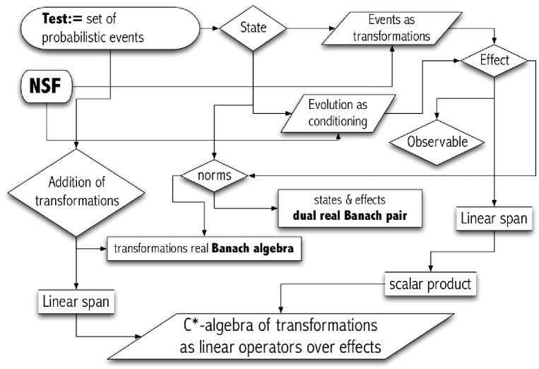
Figure 1. Logical flow chart leading to the representation of any probabilistic theory in terms of a C^∗-algebra of linear transformations over the linear space of complex effects (see also Footnote 28 and Subsect. 3.3 for an operational basis for the scalar product).

Conversely, given (1) a C^∗-algebra ${\mathfrak{T}}_{\mathbb{C}}$, (2) the cone of transformations ${\mathfrak{T}}_{+}$, and (3) the vector $e\in{\mathfrak{E}}_{\mathbb{C}}$ representing the deterministic effect, we can rebuild the full probabilistic theory by constructing the cone of effects as the orbit ${\mathfrak{E}}_{+}=e\circ{\mathfrak{T}}_{+}$, and taking the cone of states ${\mathfrak{S}}_{+}$ as the dual cone of ${\mathfrak{E}}_{+}$.

3. Independent systems

3.1. Dynamical independence and marginal states

A purely dynamical notion of system independence coincides with the possibility of performing local tests. To be precise, we will call systems ${\sf S}_{1}$ and ${\sf S}_{2}$ independent if it is possible to perform their tests as local tests, i.e. in such a way that for every joint state of ${\sf S}_{1}$ and ${\sf S}_{2}$ the transformations on ${\sf S}_{1}$ commute with transformations on ${\sf S}_{2}$, namely

(14) $$\mathscr{A}^{(1)}\circ\mathscr{B}^{(2)}=\mathscr{B}^{(2)}\circ\mathscr{A}^{(1)},\;\forall\mathscr{A}^{(1)}\in\mathbb{A}^{(1)},\,\forall\mathscr{B}^{(2)}\in\mathbb{B}^{(2)}.$$

The local tests comprise the Cartesian product ${\sf S}_{1}\times{\sf S}_{2}$, which is closed under cascade. We will close this set also under convex combination, coarse-graining and conditioning, making it a “system”, and denote such a system with the same symbol ${\sf S}_{1}\times{\sf S}_{2}$, and call local all tests in ${\sf S}_{1}\times{\sf S}_{2}$. We now compose the two systems ${\sf S}_{1}$ and ${\sf S}_{2}$ into the bipartite system ${\sf S}_{1}\odot{\sf S}_{2}$ by adding the local tests into the new system ${\sf S}_{1}\odot{\sf S}_{2}$ as ${\sf S}_{1}\odot{\sf S}_{2}\supseteq{\sf S}_{1}\times{\sf S}_{2}$ and closing under cascading, coarse-graining and convex combination. We call the tests in ${\sf S}_{1}\odot{\sf S}_{2}\setminus{\sf S}_{1}\times{\sf S}_{2}$ non-local, and we will extend the local/non-local nomenclature to the pertaining transformations. In the following for identical systems we will also use the notation ${\sf S}^{\odot N}={\sf S}\odot{\sf S}\odot\ldots\odot{\sf S}$ ($N$ times), and ${\mathfrak{Z}}^{\odot N}:={\mathfrak{Z}}({\sf S}^{\odot N})$ to denote $N$-partite sets/spaces, with $\mathfrak{Z}={\mathfrak{S}},{\mathfrak{S}}_{+},{\mathfrak{S}}_{\mathbb{R}},{\mathfrak{S}}_{\mathbb{C}},{\mathfrak{E}},{\mathfrak{E}}_{+},\ldots$

Since the local transformations commute, we will just put them in a string, as $(\mathscr{A},\mathscr{B},\mathscr{C},\ldots):=\mathscr{A}^{(1)}\circ\mathscr{A}^{(2)}\circ\mathscr{A}^{(3)}\circ\ldots$ (convex combinations and coarse graining will be sums of strings). Clearly, since the probability $\omega(\mathscr{A},\mathscr{B},\mathscr{C},\ldots)$ is independent of the time ordering of transformations, it is just a function only of the effects $\omega(\mathscr{A},\mathscr{B},\mathscr{C},\ldots)=\omega([\mathscr{A}]_{\rm eff},[\mathscr{B}]_{\rm eff},[\mathscr{C}]_{\rm eff},\ldots)$, namely the joint effect corresponding to local transformations is made of (sums of) local effects $[(\mathscr{A},\mathscr{B},\mathscr{C},\ldots)]_{\rm eff}\equiv([\mathscr{A}]_{\rm eff},[\mathscr{B}]_{\rm eff},[\mathscr{C}]_{\rm eff},\ldots)$.

The embedding of local tests ${\sf S}_{1}\times{\sf S}_{2}$ into the bipartite system ${\sf S}_{1}\odot{\sf S}_{2}$ implies that ${\mathfrak{T}}_{\mathbb{F}}({\sf S}_{1}\odot{\sf S}_{2})\supseteq{\mathfrak{T}}_{\mathbb{F}}({\sf S}_{1})\otimes{\mathfrak{T}}_{\mathbb{F}}({\sf S}_{2})$ and ${\mathfrak{E}}_{\mathbb{F}}({\sf S}_{1}\odot{\sf S}_{2})\supseteq{\mathfrak{E}}_{\mathbb{F}}({\sf S}_{1})\otimes{\mathfrak{E}}_{\mathbb{F}}({\sf S}_{2})$, both for real and complex spans $\mathbb{F}=\mathbb{R},\mathbb{C}$. On the other hand, since local tests include local state-preparation (or, otherwise, because of the no-restriction hypothesis for states) the set of bipartite states ${\mathfrak{S}}({\sf S}_{1}\odot{\sf S}_{2})$ always includes the factorized states, i.e. those corresponding to factorized probability rules e.g. $\Omega(a,b)=\omega_{1}(a)\omega_{2}(b)$ for local effects $a$ and $b$. In parallel with local transformations and effects, we will denote factorized states as strings $\Omega=(\omega_{1},\omega_{2},\ldots)$, e.g. $(\omega_{1},\omega_{2})(a,b)=\omega_{1}(a)\omega_{2}(b)$. Then, closure under convex combination implies that ${\mathfrak{S}}_{\mathbb{F}}({\sf S}_{1}\odot{\sf S}_{2})\supseteq{\mathfrak{S}}_{\mathbb{F}}({\sf S}_{1})\otimes{\mathfrak{S}}_{\mathbb{F}}({\sf S}_{2})$, for $\mathbb{F}=\mathbb{R},\mathbb{C}$.

For $N$ systems in the joint state $\Omega$, we define the marginal state $\Omega|_{n}$ of the $n$-th system the probability rule for any local transformation $\mathscr{A}$ at the $n$-th system, with all other systems untouched, namely

(15) $$\Omega|_{n}(\mathscr{A})\doteq\Omega(\mathscr{I},\ldots,\mathscr{I},\underbrace{\mathscr{A}}_{n\text{th}},\mathscr{I},\ldots).$$

Clearly, since the probability for local transformations depends only on their respective effects, the marginal state is equivalently defined as

(16) $$\Omega|_{n}(a)\doteq\Omega(e,\ldots,e,\underbrace{a}_{n\text{th}},e,\ldots)\quad\text{for }a\in{\mathfrak{E}}.$$

It readily follows that the marginal state $\Omega|_{n}$ is independent of any deterministic transformation—i.e. any test—that is performed on systems different from the $n$th: this is exactly the general statement of the no-signaling or acausality of local tests. Therefore, the present notion of dynamical independence directly implies no-signaling. The definition in Eq. (15) can be trivially extended to unnormalized states. $\!\!{}^{,}$

In the following we will use the following identities

(17) $$\Psi|_{2}(a)=\Psi(e,a)=\Psi(e,e\circ\mathscr{A})=(\mathscr{I},\mathscr{A})\Psi(e,e),\;\forall\mathscr{A}\in a.$$

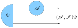
Figure 2. Illustration of the notions of dynamically (left figure) and preparationally (right figure) faithful state for a bipartite system. A bipartite state $\Phi$ is dynamically faithful with respect to system ${\sf S}_{1}$ when the output state $(\mathscr{A},\mathscr{I})\Phi$ is in one-to-one correspondence with the local transformation $\mathscr{A}$ on system ${\sf S}_{1}$, whereas it is preparationally faithful with respect to ${\sf S}_{1}$ if every bipartite state $\Psi$ can be achieved as $\Psi=(\mathscr{T}_{\Psi},\mathscr{I})\Phi$ via a local transformation $\mathscr{T}_{\Psi}$ on ${\sf S}_{1}$.

3.2. Faithful states

A bipartite state $\Phi\in{\mathfrak{S}}({\sf S}_{1}\odot{\sf S}_{2})$ is dynamically faithful with respect to ${\sf S}_{1}$ when the output state $(\mathscr{A},\mathscr{I})\Phi$ is in one-to-one correspondence with the local transformation $\mathscr{A}$ on system ${\sf S}_{1}$, that is the cone-homomorphism $\mathscr{A}\leftrightarrow(\mathscr{A},\mathscr{I})\Phi$ from ${\mathfrak{T}}_{+}({\sf S}_{1})$ to ${\mathfrak{S}}_{+}({\sf S}_{1}\odot{\sf S}_{2})$ is a monomorphism. Equivalently the map $\mathscr{A}\mapsto(\mathscr{A},\mathscr{I})\Phi$ extends to an injective linear map between the linear spaces ${\mathfrak{T}}_{\mathbb{R}}({\sf S}_{1})$ to ${\mathfrak{S}}_{\mathbb{R}}({\sf S}_{1}\odot{\sf S}_{2})$ preserving the partial ordering relative to the spanning cones, and this is true also in the inverse direction on the range of the map. Notice that no physical transformation $\mathscr{A}\neq 0$ “annihilates” $\Phi$, i.e. giving $(\mathscr{A},\mathscr{I})\Phi=0$.

A bipartite state $\Phi\in{\mathfrak{S}}({\sf S}_{1}\odot{\sf S}_{2})$ is called preparationally faithful with respect to ${\sf S}_{1}$ if every bipartite state $\Psi$ can be achieved as $\Psi=(\mathscr{T}_{\Psi},\mathscr{I})\Phi$ by a local transformation $\mathscr{T}_{\Psi}\in{\mathfrak{T}}_{+}({\sf S}_{1})$. This means that the cone-homomorphism $\mathscr{A}\mapsto(\mathscr{A},\mathscr{I})\Phi$ from ${\mathfrak{T}}_{+}({\sf S}_{1})$ to ${\mathfrak{S}}_{+}({\sf S}_{1}\odot{\sf S}_{2})$ is an epimorphism. Equivalently, the map $\mathscr{A}\mapsto(\mathscr{A},\mathscr{I})\Phi$ extends to a surjective linear map between the linear spaces ${\mathfrak{T}}_{\mathbb{R}}({\sf S}_{1})$ to ${\mathfrak{S}}_{\mathbb{R}}({\sf S}_{1}\odot{\sf S}_{2})$ preserving the partial ordering relative to the spanning cones.

In simple words, a dynamically faithful state keeps the imprinting of a local transformation on the output, i.e. from the output we can recover the transformation. On the other hand, a preparationally faithful state allows to prepare any desired joint state (probabilistically) by means of local transformations. Dynamical and preparational faithfulness correspond to the properties of being separating and cyclic for the C^∗-algebra of transformations.

Theorem 2.

The following assertions hold:

1. Any state $\Phi\in{\mathfrak{S}}({\sf S}_{1}\odot{\sf S}_{2})$ that is preparationally faithful with respect to ${\sf S}_{1}$ is dynamically faithful with respect to ${\sf S}_{2}$.

2. For identical systems in finite dimensions any state $\Phi$ that is preparationally faithful with respect to a system is also dynamically faithful with respect to the same system, and one has the cone-isomorphism ${\mathfrak{T}}_{+}({\sf S})\simeq{\mathfrak{S}}_{+}({\sf S}^{\odot 2})$. Moreover, a local transformation on $\Phi$ produces an output pure (unnormalized) bipartite state iff the transformation is atomic.

3. If there exists a state of ${\sf S}_{1}\odot{\sf S}_{2}$ that is preparationally faithful with respect to ${\sf S}_{1}$, then $\dim({\sf S}_{1})\geqslant\dim({\sf S}_{2})$.

4. If there exists a state of ${\sf S}_{1}\odot{\sf S}_{2}$ that is preparationally faithful with respect to both systems, then one has the cone-isomorphisms ${\mathfrak{E}}_{+}({\sf S}_{1})\simeq{\mathfrak{S}}_{+}({\sf S}_{2})$ and ${\mathfrak{E}}_{+}({\sf S}_{2})\simeq{\mathfrak{S}}_{+}({\sf S}_{1})$.

5. If for two identical systems there exists a state that is preparationally faithful with respect to both systems, then one has the cone-isomorphism ${\mathfrak{S}}_{+}\simeq{\mathfrak{E}}_{+}$ (weak self-duality).

6. If the state $\Phi\in{\mathfrak{S}}({\sf S}_{1}\odot{\sf S}_{2})$ is preparationally faithful with respect to ${\sf S}_{1}$, for any invertible transformation $\mathscr{A}\in{\mathfrak{T}}_{+}({\sf S}_{1})$ also the (unnormalized) state $(\mathscr{A},\mathscr{I})\Phi$ is preparationally faithful with respect to the same system. In particular, it will be a faithful state for any physical automorphism of ${\mathfrak{S}}({\sf S}_{1})$.

7. For identical systems in finite dimensions, for $\Phi$ preparationally faithful with respect to both systems, the state $\chi:=\Phi(e,\cdot)$ is cyclic in ${\mathfrak{S}}_{+}({\sf S})$ under ${\mathfrak{T}}_{+}({\sf S})$, and the observables $\mathbb{L}=\{l_{i}\}$ of ${\sf S}_{2}$ are in one-to-one correspondence with the ensemble decompositions $\{\rho_{i}\}_{i=1}^{|\mathbb{L}|}$ of $\chi$, with $\rho_{i}:=\Phi(l_{i},\cdot)$, and $\chi$ is an internal state.

Proof.

1. Introduce the map $\omega\mapsto\mathscr{T}_{\omega}$ where for every $\omega\in{\mathfrak{S}}({\sf S}_{2})$ one chooses a local transformation $\mathscr{T}_{\omega}$ on ${\sf S}_{1}$ such that $(\mathscr{T}_{\omega},\mathscr{I})\Phi|_{2}=\omega$. This is possible because $\Phi$ is preparationally faithful with respect to ${\sf S}_{1}$. One has $\mathscr{A}\omega=(\mathscr{T}_{\omega},\mathscr{A})\Phi|_{2}=(\mathscr{T}_{\omega},\mathscr{I})(\mathscr{I},\mathscr{A})\Phi|_{2}$ $\forall\omega\in{\mathfrak{S}}({\sf S}_{2})$. Therefore, from $(\mathscr{I},\mathscr{A})\Phi$ one can recover the action of $\mathscr{A}$ on any state $\omega$ by first applying $(\mathscr{T}_{\omega},\mathscr{I})$ and then take the marginal, i.e. one recovers $\mathscr{A}$ from $(\mathscr{I},\mathscr{A})\Phi$, which is another way of saying that $\mathscr{A}\mapsto(\mathscr{I},\mathscr{A})\Phi$ is injective, namely $\Phi$ is dynamically faithful with respect to ${\sf S}_{2}$.

2. Denote by $\Phi\in{\mathfrak{S}}^{\odot 2}$ a state that is preparationally faithful with respect to ${\sf S}_{1}$. Since the linear map $\mathscr{A}\mapsto(\mathscr{A},\mathscr{I})\Phi$ from ${\mathfrak{T}}_{\mathbb{R}}$ to ${\mathfrak{S}}_{\mathbb{R}}^{\odot 2}$ is surjective, one has $\dim({\mathfrak{T}}_{\mathbb{R}})\geqslant\dim({\mathfrak{S}}_{\mathbb{R}}^{\odot 2})$. However, one has also $\dim({\mathfrak{T}}_{\mathbb{R}})\leqslant\dim({\mathfrak{S}}_{\mathbb{R}}^{\odot 2})$ since ${\mathfrak{T}}_{\mathbb{R}}\subseteq{\sf Lin({\mathfrak{S}}_{\mathbb{R}})}\simeq{\mathfrak{S}}_{\mathbb{R}}^{\otimes 2}\subseteq{\mathfrak{S}}_{\mathbb{R}}^{\odot 2}$, whence $\dim({\mathfrak{T}}_{\mathbb{R}})=\dim({\mathfrak{S}}_{\mathbb{R}}^{\odot 2})$, and, having null kernel, the map is also injective, whence $\Phi$ is dynamically faithful with respect to ${\sf S}_{1}$. Since now the state $\Phi$ is both preparationally and dynamically faithful with respect to the same system ${\sf S}_{1}$, it follows that the map $\mathscr{A}\mapsto(\mathscr{A},\mathscr{I})\Phi$ establishes the cone-isomorphism ${\mathfrak{T}}_{+}\simeq{\mathfrak{S}}_{+}^{\odot 2}$. Since the faithful state establishes the cone-isomorphism ${\mathfrak{T}}_{+}\simeq{\mathfrak{S}}_{+}^{\odot 2}$, it maps extremal rays of ${\mathfrak{T}}_{+}$ to extremal rays of ${\mathfrak{S}}_{+}^{\odot 2}$ and vice-versa, that is $\mathscr{A}\in{\sf Erays}({\mathfrak{T}}_{+})$ iff $(\mathscr{A},\mathscr{I})\Phi\in{\sf Erays}({\mathfrak{S}}_{+}^{\odot 2})$.

3. For $\Phi$ preparationally faithful with respect to ${\sf S}_{1}$, consider the cone homomorphism $a\mapsto\omega_{a}:=\Phi(a,\cdot)$ which associates an (un-normalized) state $\omega_{a}\in{\mathfrak{S}}_{+}({\sf S}_{2})$ to each effect $a\in{\mathfrak{E}}_{+}({\sf S}_{1})$. The extension to a linear map $a\mapsto\omega_{a}$ between the linear spaces ${\mathfrak{S}}_{\mathbb{R}}({\sf S}_{2})$ and ${\mathfrak{E}}_{\mathbb{R}}({\sf S}_{1})$ preserves the cone structure, and is surjective, since $\Phi$ is preparationally faithful with respect to ${\sf S}_{1}$ (whence every bipartite state, and in particular every marginal state, can be obtained from a local effect). The bound $\dim({\sf S}_{1})\geqslant\dim({\sf S}_{2})$ then follows from surjectivity.

4. Similarly to the proof of item (1), consider the map $\lambda\mapsto\mathscr{T}_{\lambda}$ where for every marginal state $\lambda\in{\mathfrak{S}}({\sf S}_{1})$ one chooses a local transformation $\mathscr{T}_{\lambda}$ on ${\sf S}_{2}$ such that $(\mathscr{I},\mathscr{T}_{\lambda})\Phi|_{1}=\lambda$ ($\Phi$ is preparationally faithful with respect to ${\sf S}_{2}$). Then, one has

   (18) $$\forall\lambda\in{\mathfrak{S}}({\sf S}_{1}),\quad\lambda(a)=(\mathscr{I},\mathscr{T}_{\lambda})\Phi(a,e)=\Phi(a,\mathscr{T}_{\lambda})=\omega_{a}(\mathscr{T}_{\lambda}).$$

   It follows that $\omega_{a}=\omega_{b}$ implies that $\lambda(a)=\lambda(b)$ for all states $\lambda\in{\mathfrak{S}}({\sf S}_{1})$, that is $a=b$, whence the homomorphism $a\mapsto\omega_{a}$ which is surjective (since $\Phi$ is preparationally faithful) is also injective, i.e. is bijective, and since it maps elements of ${\mathfrak{E}}_{+}({\sf S}_{1})$ to elements of ${\mathfrak{S}}_{+}({\sf S}_{2})$ and, vice-versa, to each element of ${\mathfrak{S}}_{+}({\sf S}_{2})$ it corresponds an element of ${\mathfrak{E}}_{+}({\sf S}_{1})$ ($\Phi$ is preparationally faithful), it is a cone-isomorphism. We then have the cone-isomorphism ${\mathfrak{E}}_{+}({\sf S}_{1})\simeq{\mathfrak{S}}_{+}({\sf S}_{2})$. The cone-isomorphism ${\mathfrak{E}}_{+}({\sf S}_{2})\simeq{\mathfrak{S}}_{+}({\sf S}_{1})$ follows by exchanging the two systems.

5. According to point (4) one has the cone-isomorphism ${\mathfrak{E}}_{+}({\sf S}_{1})\simeq{\mathfrak{S}}_{+}({\sf S}_{2})\simeq{\mathfrak{S}}_{+}({\sf S}_{1})$.

6. Obvious, by definition of preparationally faithful state.

7. According to (4) $\omega_{a}:=\Phi(a,\cdot)$ establishes the cone-isomorphism ${\mathfrak{E}}_{+}({\sf S})\simeq{\mathfrak{S}}_{+}({\sf S})$. On the other hand, since the state is both preparationally and dynamically faithful for either systems, then for any transformation $\mathscr{T}$ on the first system there exists a unique transformation $\mathscr{T}^{\prime}$ on the other system giving the same output state (see also the definition of the “transposed” transformation with respect to a dynamically faithful state in the following). Therefore, since any effect $a$ can be written as $a=e\circ\mathscr{T}_{a}$ for any $\mathscr{T}_{a}\in a$, one has $\omega_{a}=\Phi(e\circ\mathscr{T}_{a},\cdot)=\Phi(e,\cdot\circ\mathscr{T}_{a}^{\prime})=\mathscr{T}_{a}^{\prime}\chi$. The observable-ensemble correspondence and the fact that $\chi$ is an internal state are both immediate consequence of the fact that $\omega_{a}:=\Phi(a,\cdot)$ is a cone-isomorphism. $\,\blacksquare$

Transposed of a transformation

For a symmetric bipartite state $\Phi$ of two identical systems that is preparationally faithful for one system—hence, according to Theorem 2, is both dynamically and preparationally faithful with respect to both systems—one can define operationally the transposed $\mathscr{T}^{\prime}$ of a transformation $\mathscr{T}\in{\mathfrak{T}}_{\mathbb{R}}$ through the identity

(19) $$\Phi(a,b\circ\mathscr{T})=\Phi(a\circ\mathscr{T}^{\prime},b),$$

i.e. $(\mathscr{T}^{\prime},\mathscr{I})\Phi=(\mathscr{I},\mathscr{T})\Phi$, namely, operationally the transposed $\mathscr{T}^{\prime}$ of a transformation $\mathscr{T}$ is the transformation which will give the same output bipartite state of $\mathscr{T}$ if operated on the twin system. It is easy to verify (using symmetry of $\Phi$) that $\mathscr{T}^{\prime\prime}=\mathscr{T}$ and that $(\mathscr{B}\circ\mathscr{A})^{\prime}=\mathscr{A}^{\prime}\circ\mathscr{B}^{\prime}$.

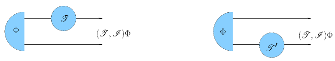
Figure 3. Illustration of the notions of transposed of a transformation for a symmetric dynamically and preparationally faithful state.

We are now in position to formulate the main Postulate:

Postulate PFAITH (Existence of a symmetric preparationally-faithful pure state). For any couple of identical systems, there exist a symmetric (under permutation of the two systems) pure state that is preparationally faithful.

Theorem 2 guarantees that such a state is both dynamically and preparationally faithful, and with respect to both systems, as a consequence of symmetry. Postulate PFAITH thus guarantees that to any system we can adjoin an ancilla and prepare a pure state which is dynamically and preparationally faithful with respect to our system. This is operationally crucial in guaranteeing the preparability of any quantum state for any bipartite system using only local transformations, and to assure the possibility of experimental calibrability of tests for any system. Notice that it would be impossible, even in principle, to calibrate transformations without a dynamically faithful state, since any set of input states $\{\omega_{n}\}\in{\sf S}^{\prime}$ that is “separating” for transformations ${\mathfrak{T}}({\sf S}^{\prime})$ is equivalent to a bipartite state $\Phi=\sum_{n}\omega_{n}\otimes\lambda_{n}\in{\mathfrak{S}}({\sf S}^{\prime}\odot{\sf S}^{\prime\prime})$ which is dynamically faithful for ${\sf S}^{\prime}$, with the states $\{\lambda_{n}\}$ working just as “flags” representing the “knowledge” of which state of the set $\{\omega_{n}\}$ has been prepared. Notice that in QM every maximal Schmidt-number entangled state of two identical systems is both preparationally and dynamically faithful for both systems. In classical mechanics, on the other hand, a state of the form $\Phi=\sum_{l}|l\rangle\langle l|\otimes|l\rangle\langle l|$ with $\{|l\rangle\}$ complete orthogonal set of states (see footnote 20) will be both dynamically and preparationally faithful, however, being not pure, it would require a (possibly unlimited) sequence of preparations.

On the mathematical side, instead, according to Theorem 2 Postulate PFAITH restricts the theory to the weakly self-dual scenario (i.e. with the cone-isomorphism ${\mathfrak{S}}_{+}\simeq{\mathfrak{E}}_{+}$), and in finite dimensions one also has the cone-isomorphism ${\mathfrak{T}}_{+}({\sf S})\simeq{\mathfrak{S}}_{+}({\sf S}^{\odot 2})$. In addition, one also has the following very useful lemma.

Lemma 5.

For finite dimensions Postulate PFAITH implies that the linear space of transformations is full, i.e. ${\mathfrak{T}}_{\mathbb{F}}={\sf Lin({\mathfrak{E}}_{\mathbb{F}})}$. Moreover, one has ${\mathfrak{S}}_{\mathbb{F}}({\sf S}^{\odot 2})={\mathfrak{S}}_{\mathbb{F}}({\sf S})^{\otimes 2}$ and ${\mathfrak{E}}_{\mathbb{F}}({\sf S}^{\odot 2})={\mathfrak{E}}_{\mathbb{F}}({\sf S})^{\otimes 2}$ for $\mathbb{F}=\mathbb{R},\mathbb{C}$, that is bipartite states and effects are cones spanning the tensor products ${\mathfrak{S}}_{\mathbb{F}}^{\otimes 2}$ and ${\mathfrak{E}}_{\mathbb{F}}^{\otimes 2}$, respectively.

Proof. In the following we restrict to finite dimensions, with $\mathbb{F}=\mathbb{R},\mathbb{C}$ denoting either the real or the complex fields, respectively. According to item (2) of Theorem 2, for two identical systems the existence of a state that is preparationally faithful with respect to either one of the two systems implies ${\mathfrak{S}}_{\mathbb{F}}({\sf S}^{\odot 2})\simeq{\mathfrak{T}}_{\mathbb{F}}({\sf S})$. Since transformations act linearly over effects one has ${\mathfrak{T}}_{\mathbb{F}}\subseteq{\sf Lin({\mathfrak{E}}_{\mathbb{F}})}\simeq{\mathfrak{E}}_{\mathbb{F}}^{\otimes 2}$, whence ${\mathfrak{E}}_{\mathbb{F}}({\sf S}^{\odot 2})\simeq{\mathfrak{S}}_{\mathbb{F}}({\sf S}^{\odot 2})\simeq{\mathfrak{T}}_{\mathbb{F}}({\sf S})\subseteq{\mathfrak{E}}_{\mathbb{F}}({\sf S})^{\otimes 2}$. However, by local-test embedding one also has ${\mathfrak{E}}_{\mathbb{F}}({\sf S}^{\odot 2})\supseteq{\mathfrak{E}}_{\mathbb{F}}({\sf S})^{\otimes 2}$, whence ${\mathfrak{E}}_{\mathbb{F}}({\sf S}^{\odot 2})={\mathfrak{E}}_{\mathbb{F}}({\sf S})^{\otimes 2}$, which implies that ${\mathfrak{T}}_{\mathbb{F}}={\sf Lin({\mathfrak{E}}_{\mathbb{F}})}$. Finally, by state-effect duality one also has ${\mathfrak{S}}_{\mathbb{F}}({\sf S}^{\odot 2})={\mathfrak{S}}_{\mathbb{F}}^{\otimes 2}({\sf S})$. $\,\blacksquare$

The above lemma could have been extended to couples of different systems. However, this would necessitate with the consideration of more general transformations between different systems (see Footnote 14).

We conclude that Postulate PFAITH—i.e. the existence of a symmetric preparationally-faithful pure state for bipartite systems—guarantees that we can represent bipartite quantities (states, effects, transformations) as elements of the tensor product of the single-system spaces. This fact also implies the following relevant principle

Corollary 2 (Local observability principle).

For every composite system there exist informationally complete observables made of local informationally complete observables.

Proof. A joint observable made of local observables $\mathbb{L}=\{l_{i}\}$ on ${\sf S}_{1}$ and $\mathbb{M}=\{m_{j}\}$ on ${\sf S}_{2}$ is of the form $\mathbb{L}\times\mathbb{M}=\{(l_{i},m_{j})\}$. Then, by definition, the statement of the corollary is ${\mathfrak{E}}_{\mathbb{R}}({\sf S}^{\odot 2})\subseteq{\sf Span}_{\mathbb{R}}(\mathbb{L}\times\mathbb{M})={\mathfrak{E}}_{\mathbb{R}}^{\otimes 2}({\sf S})$, which is true according to Lemma 5. $\,\blacksquare$

Operationally, the Local Observability Principle plays a crucial role, since it reduces enormously experimental complexity, by guaranteeing that only local (although jointly executed) tests are sufficient to retrieve a complete information of a composite system, including all correlations between the components. This principle reconciles holism with reductionism in a non-local theory, in the sense that we can observe a holistic nature in a reductionistic way, i.e. locally.

In addition to Lemma 5 and to the local observability principle, Postulate PFAITH has a long list of remarkable consequences for the probabilistic theory, which are given by the following theorem.

Theorem 3.

If PFAITH holds, the following assertions are true

1. The identity transformation is atomic.

2. One has $\omega_{a\circ\mathscr{A}^{\prime}}=\mathscr{A}\omega_{a}$, or equivalently $\mathscr{A}\omega=\Phi(a_{\omega}\circ\mathscr{A}^{\prime},\cdot)$, where $\mathscr{A}^{\prime}$ denotes the transposed of $\mathscr{A}$ with respect to $\Phi$.

3. The transpose of a physical automorphism of the set of states is still a physical automorphism of the set of states.

4. The marginal state $\chi$ is invariant under the transpose of a channel (deterministic transformation) whence, in particular, under a physical automorphism of the set of states.

5. Alice’s can perform a perfect EPR-cheating in a perfect concealing bit commitment protocol.

Proof.

1. According to Theorem 2-2, the map $\mathscr{A}\mapsto(\mathscr{A},\mathscr{I})\Phi$ establishes the cone-isomorphism ${\mathfrak{T}}_{+}\simeq{\mathfrak{S}}_{+}^{\odot 2}$, whence mapping extremal rays of ${\mathfrak{T}}_{+}$ to extremal rays of ${\mathfrak{S}}_{+}^{\odot 2}$ and vice-versa it maps the state $\Phi$ itself (which is pure) to the identity, which then must be atomic.

2. Immediate definition of the transposition with respect to the dynamically faithful state $\Phi$.

3. Point (2) establishes that the transposed of a state-automorphism is an effect automorphism, which, due to the cone-isomorphism, is again a state-automorphism (see also footnote 36).

4. For deterministic $\mathscr{T}$ one has $\mathscr{T}^{\prime}\chi=\Phi(e,\cdot\circ\mathscr{T}^{\prime})=\Phi(e\cdot\mathscr{T},\cdot)=\Phi(e,\cdot)=\chi$. The last statement follows from (3) (see also footnote 36).

5. [For the definition of the protocol, see Ref.[38]]. For the protocol to be concealing there must exist two ensembles of states $\{\rho_{i}^{\mathbb{A}}\}$ and $\{\rho_{i}^{\mathbb{B}}\}$ that are indistinguishable by Bob. These correspond to the two observables $\mathbb{A}=\{a_{i}\}$ and $\mathbb{B}=\{b_{i}\}$ with $\rho_{i}^{\mathbb{A}}=\Phi(a_{i},\cdot)$ and $\rho_{i}^{\mathbb{B}}=\Phi(b_{i},\cdot)$. Instead of sending to Bob a state from either one of the two ensembles, Alice can cheat by “entangling” her ancilla (system ${\sf S}_{1}$) with Bob system in the state $\Phi$, and then measuring either one of the observables $\mathbb{A}=\{a_{i}\}$ and $\mathbb{B}=\{b_{i}\}$.$\,\blacksquare$

Notice that atomicity of identity occurs in QM, whereas it is not true in a classical probabilistic theory (see Footnote 20). In classical mechanics one can gain information on the state without making disturbance thanks to non-atomicity of the identity transformation. According to Theorem 3-1 the need of disturbance for gaining information is a consequence of the purity of the preparationally faithful state, whence disturbance is the price to be payed for the reduction of the preparation complexity.

3.3. Scalar product over effects induced by a symmetric faithful state

In this subsection I briefly review the construction in Ref. [17] of a scalar product over ${\mathfrak{E}}_{\mathbb{C}}$ via a symmetric faithful state, along with the corresponding operational definition of “transposed” and “complex conjugation”—with the composition of the two giving the adjoint.

According to Theorem 2-2, for two identical systems in finite dimensions any state that is preparationally faithful with respect to a system is also dynamically faithful with respect to the same system. Moreover, according to Postulate PFAITH, there always exists such a state, say $\Phi$, which is symmetric under permutation of the two systems. The state $\Phi$ is then a symmetric real form over ${\mathfrak{E}}_{\mathbb{R}}$, whence it provides a non-degenerate scalar product over ${\mathfrak{E}}_{\mathbb{R}}$ via its Jordan form

(20) $$\forall a,b\in{\mathfrak{E}}_{\mathbb{R}},\quad{}_{\Phi}(b|a)_{\Phi}:=|\Phi|(b,a)=\Phi(\varsigma(b),a),$$

where $\varsigma$ is the involution $\varsigma=\pi_{+}-\pi_{-}$, $\pi_{\pm}$ denoting the orthogonal projectors over the positive (negative) eigenspaces of the symmetric form, or, explicitly, $\varsigma(a):=\sum_{j}\Phi(a,\tilde{f}_{j})\tilde{f}_{j}$ and $\{\tilde{f}_{j}\}$ is the canonical Jordan basis. Notice that the Jordan form is representation-dependent—i.e. it is defined through the reference test $\mathbb{L}=\{l_{i}\}$—whereas its signature—i.e. the difference between the numbers of positive and negative eigenvalues—will be a property of the system ${\sf S}$, and will generally depend on the specific probabilistic theory. For transformations $\mathscr{T}\in{\mathfrak{T}}_{\mathbb{R}}$ we define $a\circ\varsigma(\mathscr{T}):=\varsigma(\varsigma(a)\circ\mathscr{T})=:a\circ\mathscr{Z}\circ\mathscr{T}\circ\mathscr{Z}$. For the identity transformation we have $\varsigma(\mathscr{I})=\mathscr{Z}\circ\mathscr{Z}=\mathscr{I}$. Corresponding to a symmetric faithful bipartite state $\Phi$ one has the generalized transformation $\mathscr{T}_{\Phi}$, given by

(21) $$a\circ\mathscr{T}_{\Phi}:=\sum_{k}\Phi(l_{k},a)l_{k},$$

for a fixed orthonormal basis $\mathbb{L}=\{l_{j}\}$, and in terms of the corresponding symmetric scalar product $(\cdot,\cdot)_{\mathbb{L}}$ introduced in Subsection 2.10, one has

(22) $$(a,b\circ\mathscr{T}_{\Phi})_{\mathbb{L}}=(a\circ\mathscr{T}_{\Phi},b)_{\mathbb{L}}=\Phi(a,b).$$

Using the dynamical and preparational faithfulness of $\Phi$ we have defined operationally the transposed $\mathscr{T}^{\prime}$ of a transformation $\mathscr{T}\in{\mathfrak{T}}_{\mathbb{R}}$. Such “operational” transposed is related to the transposed $\tilde{\mathscr{C}}$ under the scalar product $(\cdot,\cdot)_{\mathbb{L}}$ as $\mathscr{C}^{\prime}=\mathscr{T}_{\Phi}\circ\tilde{\mathscr{C}}\circ\mathscr{T}_{\Phi}^{-1}$. It is easy to check that $\tilde{\mathscr{Z}}=\mathscr{Z}=\mathscr{Z}^{\prime}$.

On the complex linear span ${\mathfrak{T}}_{\mathbb{C}}$ one can introduce a scalar product as the sesquilinear extension of the real symmetric scalar product $(\cdot,\cdot)_{\Phi}$ over ${\mathfrak{E}}_{\mathbb{R}}$ via the complex conjugation $\eta(\mathscr{T})=\mathscr{T}_{R}-i\mathscr{T}_{I}$, $\mathscr{T}_{R,I}\in{\mathfrak{T}}_{\mathbb{R}}$, and the adjoint for the sesquilinear scalar product is then given by

(23) $$\mathscr{T}^{\dagger}=\mathscr{Z}\circ\eta(\mathscr{T}^{\prime})\circ\mathscr{Z}=|\mathscr{T}_{\Phi}|\circ\eta(\tilde{\mathscr{T}})\circ|\mathscr{T}_{\Phi}|^{-1},$$

namely $\mathscr{T}^{\dagger}=\mathscr{Z}\circ\mathscr{T}^{\prime}\circ\mathscr{Z}$ on real transformations $\mathscr{T}\in{\mathfrak{T}}_{\mathbb{R}}$. The Jordan involution $\varsigma$ thus plays the role of a complex conjugation on ${\mathfrak{T}}_{\mathbb{R}}$, which must be anti-linearly extended to ${\mathfrak{T}}_{\mathbb{C}}$.

The faithful state $\Phi$ becomes a cyclic and separating vector of a GNS representation by noticing that $(\mathscr{A}^{(2)}\Phi)(\eta\varsigma b,a)={}_{\Phi}(b,a\circ\mathscr{A})_{\Phi}$, and in Eq. (23) one can recognize the Tomita-Takesaki modular operator of the representation [39].

4. Axiomatic interlude: exploring Postulates FAITHE and PURIFY

In this section we are exploring two additional postulates of a probabilistic theory: Postulate FAITHE—the existence of a faithful effect (somehow dual to Postulate PFAITH)—and Postulate PURIFY—the existence of a purification for every state. As we will see, these new postulates make the probabilistic theory closer and closer to QM. However, I was still unable to prove (nor to find counterexamples) that with these two additional postulates the probabilistic theory is QM.

4.1. FAITHE: a postulate on a faithful effect

As previously mentioned, Postulate FAITHE is somehow the dual version of Postulate PFAITH:

Postulate FAITHE (Existence of a faithful effect). There exist a bipartite effect $F\in{\mathfrak{E}}({\sf S}^{\odot 2})$ achieving the inverse of the isomorphism $a\mapsto\omega_{a}:=\Phi(a,\cdot)$. More precisely

(24) $$F_{23}(\omega_{a})_{2}=F_{23}\Phi_{12}(a,\cdot)=\alpha a_{3},\quad 0<\alpha\leqslant 1.$$

Notice that, since $\Phi$ establishes an isomorphism between the cones of states and effects, there must exist a generalized effect $F\in{\mathfrak{E}}_{\mathbb{R}}^{\otimes 2}$ satisfying Eq. (24), but we are not guaranteed that it is a physical, i.e. $F\in{\mathfrak{E}}_{+}({\sf S}^{\odot 2})$.

Let’s denote by $\hat{F}=\alpha^{-1}F$ the rescaled effect in the cone. Eq. (24) can be rewritten in different notation as follows

(25) $$\hat{F}(\omega_{a},\cdot)=\hat{F}(\Phi(a,\cdot),\cdot)=a$$

(26) $$\Phi(a_{\omega},\cdot)=\Phi(\hat{F}(\omega,\cdot),\cdot)=\omega.$$

[One needs to be careful with the notation in the multipartite case, e.g. in Eq. (26) $\Phi(\hat{F}(\omega,\cdot),\cdot)=\omega$ is actually a state, since $\hat{F}(\omega,\cdot)$ is an effect, etc.] Both faithful state $\Phi$ and faithful effect $F$ can be used to express the state-effect pairing, namely

(27) $$\zeta(b)=\Phi(a_{\zeta},b)=\hat{F}(\omega_{b},\zeta),\qquad a_{\zeta}:=\hat{F}(\zeta,\cdot),\quad\omega_{b}:=\Phi(b,\cdot),$$

or, substituting

(28) $$\zeta(b)=\Phi(\hat{F}(\zeta,\cdot),b)=\hat{F}(\Phi(b,\cdot),\zeta).$$

Eq. (24) can also be rewritten as follows

(29) $$F_{23}\Phi_{12}=\alpha\,\mathbf{Swap}_{13},$$

where $\mathbf{Swap}_{ij}$ denotes the transformation swapping ${\sf S}_{i}$ with ${\sf S}_{j}$. In Fig. 4 Postulate FAITHE is illustrated graphically.

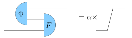
Figure 4. Illustration of Postulate FAITHE.

Eq. (29) means that using the state $\Phi$ and the effect $F$ one can achieve probabilistic teleportation of states from ${\sf S}_{2}$ to ${\sf S}_{4}$. In fact, one has

(30) $$F_{23}\omega_{2}\Phi_{34}=F_{23}\Phi_{12}(a_{\omega},\cdot)\Phi_{34}=\alpha\Phi_{14}(a_{\omega},\cdot)=\alpha\omega_{4}.$$

Using the last identity we can also see that Postulate FAITHE is also equivalent to the identity

(31) $$F_{23}\Phi_{12}\Phi_{34}=\alpha\Phi_{14},$$

which by linearity is extended from local effects to all effects, in virtue of ${\mathfrak{E}}^{\odot 2}={\mathfrak{E}}^{\otimes 2}$. With equivalent notation we can write $(\Phi,\Phi)(\cdot,F,\cdot)=\alpha\Phi$.

The effect $F$ is also completely faithful, in the sense that the correspondence $F_{\mathscr{A}}:=F\circ(\mathscr{A}^{\prime},\mathscr{I})\Longleftrightarrow\mathscr{A}$ is bijective (in finite dimensions). In fact one has

(32) $$[F\circ(\mathscr{A}^{\prime},\mathscr{I})]_{23}(\Phi,\Phi)=\alpha(\mathscr{A},\mathscr{I})\Phi,$$

and since $\Phi$ is dynamically faithful (it is symmetric preparationally faithful), the correspondence $F_{\mathscr{A}}:=F\circ(\mathscr{A}^{\prime},\mathscr{I})\Longleftrightarrow\mathscr{A}$ is one-to-one and surjective, whence it is a bijection (in finite dimensions). It is also easy to see that $F\circ(\mathscr{A}^{\prime},\mathscr{I})]=F\circ(\mathscr{I},\mathscr{A})$, since

(33) $$\begin{split}[F\circ(\mathscr{I},\mathscr{A})]_{23}(\Phi,\Phi)&=F_{23}(\Phi,(\mathscr{A},\mathscr{I})\Phi)=F_{23}(\Phi,(\mathscr{I},\mathscr{A}^{\prime})]\Phi)\\ &=\alpha(\mathscr{I},\mathscr{A}^{\prime})\Phi=\alpha(\mathscr{A},\mathscr{I})\Phi=[F\circ(\mathscr{A}^{\prime},\mathscr{I})]_{23}(\Phi,\Phi),\end{split}$$

whence transposition can be equivalently defined with respect to the faithful effect $F$. The bijection $F_{\mathscr{A}}:=F\circ(\mathscr{I},\mathscr{A})\Longleftrightarrow\mathscr{A}$ is cone-preserving in both directions, since to every transformation it corresponds an effect, and to each effect $A\in{\mathfrak{E}}({\sf S}^{\odot 2})$ it corresponds a transformation, since

(34) $$A_{23}(\Phi,\Phi)=\Omega_{A}=(\mathscr{T}_{\Omega_{A}},\mathscr{I})\Phi=:(\mathscr{T}_{A},\mathscr{I})\Phi.$$

Therefore, the map $\mathscr{A}\mapsto F_{\mathscr{A}}$ realizes the cone-isomorphism ${\mathfrak{E}}_{+}({\sf S}^{\odot 2})\simeq{\mathfrak{T}}_{+}({\sf S})$ which is just the composition of the weak-selfduality and of the isomorphism ${\mathfrak{S}}_{+}({\sf S}^{\odot 2})\\ \simeq{\mathfrak{T}}_{+}({\sf S})$ due to PFAITH. However, as mentioned in footnote 40, the map

(35) $${\mathfrak{E}}_{+}({\sf S}^{\odot 2})\ni A\mapsto\Omega_{A}:=A_{23}(\Phi,\Phi)\in{\mathfrak{S}}({\sf S}^{\odot 2}),$$

is bijective between ${\mathfrak{S}}_{\mathbb{F}}({\sf S}^{\odot 2})$ and ${\mathfrak{E}}_{\mathbb{F}}({\sf S}^{\odot 2})$, but it does not realize the cone-isomorphism ${\mathfrak{S}}_{+}({\sf S}^{\odot 2})\simeq{\mathfrak{E}}_{+}({\sf S}^{\odot 2})$, since it is not surjective over ${\mathfrak{E}}_{+}({\sf S}^{\odot 2})$. Indeed, for $A\in{\mathfrak{E}}({\sf S}^{\odot 2})$ physical effect, one has $A_{23}(\Phi,\Phi)=(\mathscr{T}_{A},\mathscr{I})\Phi$ with $\mathscr{T}_{A}\in{\mathfrak{T}}({\sf S})$ physical transformation. However, there is no guarantee that, vice-versa, a physical transformation always has a corresponding physical effect, e.g. for the identity transformation in Eq. (31). It also follows that any bipartite observable $\mathbb{A}=\{A_{l}\}$ leads to the totally depolarizing channel $\mathscr{T}_{(e,e)}\omega=\chi$, $\forall\omega\in{\mathfrak{S}}$. Using the faithfulness of $F$ it is possible to achieve probabilistically any transformation on a state $\omega$ by performing a joint test on the system interacting with an ancilla, i.e. $(\omega\Phi)(F_{\mathscr{A}^{\prime}},\cdot)=\alpha\mathscr{A}\omega$ (for Stinespring-like dilations in an operational context see Ref. [31]).

More about the constant $\alpha$

Notice that the number $0<\alpha\leqslant 1$ is the probability of achieving teleportation $\alpha=(F_{23}\omega_{2}\Phi_{34})(e)$. It is independent on the state $\omega$, and depends only on $F$, since it is given by $\alpha\equiv\alpha_{F}=[F_{23}\Phi_{12}\Phi_{34}](e,e)$. The maximum value maximized over all bipartite effects

(36) $$\alpha({\sf S})=\max_{A\in{\mathfrak{E}}({\sf S}^{\odot 2})}\{(\Phi,\Phi)(e,A,e)\}$$

is a property of the system ${\sf S}$ only, and depends on the particular probabilistic theory.

More on the relation between Postulates PFAITH and FAITHE

Postulate PFAITH guarantees the existence of a symmetric preparationally faithful state for each pair of identical systems ${\sf S}^{\odot 2}$. Now, consider the bipartite system ${\sf S}^{\odot 2}\odot{\sf S}^{\odot 2}$, and denote by ${\mathbf{\Phi}}$ a symmetric preparationally faithful state for it. The map $A\mapsto\Omega_{A}:={\mathbf{\Phi}}(A,\cdot,\cdot)$ $\forall A\in{\mathfrak{E}}({\sf S}^{\odot 2})$ establishes the state–effect cone-isomorphism for ${\sf S}^{\odot 2}$, whence there must exists an effect $A_{\Phi}$ such that

(37) $${\mathbf{\Phi}}(A_{\Phi},\cdot,\cdot)=\beta\Phi,\quad 0<\beta\leqslant 1.$$

Suppose now that the faithful state can be chosen in such a way that it maps separable states to separable effects as follows

(38) $${\mathbf{\Phi}}(\cdot,\cdot,(a,b))=\gamma(\omega_{a},\omega_{b})=\gamma\Phi(\cdot,a)\Phi(\cdot,b),\;\gamma>0.$$

Then one has

(39) $$\gamma(A_{\Phi})_{13}(\Phi,\Phi)={\mathbf{\Phi}}(A_{\Phi},\cdot,\cdot)=\beta\Phi,$$

namely, according to Eq. (31) one has $\beta^{-1}\gamma A_{\Phi}\equiv\hat{F}$, which is the effect whose existence is postulated by FAITHE. Notice, however, that the factorization Eq. (38) doesn’t need to be satisfied. In other words, the automorphism relating the cone-isomorphism induced by ${\mathbf{\Phi}}$ with another cone-isomorphism that preserves local effects may be unphysical (see also footnote 40). One can instead require a stronger version of postulate PFAITH, postulating the existence of a preparationally super-faithful symmetric state $\Phi$, also achieving a four-partite preparationally symmetric faithful state ${\mathbf{\Phi}}$ as $(\Phi,\Phi)={\mathbf{\Phi}}$. A weaker version of such postulate is thoroughly analyzed in Ref. [31], where it is also shown that it leads to Stinespring-like dilations of deterministic transformations.

The case of QM

It is a useful exercise to see how the present framework translates in the quantum case, and find which additional constraints can arise from a specific probabilistic theory. For simplicity we consider a maximally entangled state (with all positive amplitudes in a fixed basis) as a preparationally symmetric state $\Phi$. The corresponding marginal state is given by the density matrix $d^{-1}I$, $I$ denoting the identity on the Hilbert space. For the constant $\alpha$ one has $\alpha=d^{-2}$, where $d$ is the dimension of the Hilbert space. A simple calculation shows that the identity $\omega_{a}=\mathscr{T}_{a}^{\prime}\chi$ for $\mathscr{T}_{a}\in a$ translates to

(40) $$\omega_{a}=\sqrt{\alpha}\varsigma(a),\qquad\Leftarrow\text{in QM}$$

where the involution $\varsigma$ of the Jordan form in Eq. $\Phi$ (20) here is also an automorphism of states/effects, whence identity (40) expresses the self-duality of QM. Rewriting Eq. (40) in terms of the faithful effect $F$ (which would be an element of a Bell measurement), one obtains

(41) $$(\cdot,F)(\Phi,\cdot)=\sqrt{\alpha}|\Phi|,\qquad\Leftarrow\text{in QM}.$$

Another feature of QM is that the preparationally faithful symmetric state $\Phi$ is super-faithful, namely ${\mathbf{\Phi}}=(\Phi,\Phi)$ is preparationally faithful for ${\sf S}^{\odot 4}$.

4.2. PURIFY: a postulate on purifiability of all states

In the present section for completeness I briefly explore the consequences of assuming purifiability for all states, namely:

Postulate PURIFY (Purifiability of states). For every state $\omega$ of ${\sf S}$ there exist a pure bipartite state $\Omega$ of ${\sf S}^{\odot 2}$ having it as marginal state, namely

(42) $$\forall\omega\in{\mathfrak{S}}({\sf S}),\;\exists\Omega\in{\mathfrak{S}}({\sf S}^{\odot 2})\text{ pure, such that }\Omega(e,\cdot)=\omega.$$

Postulate PURIFY has been analyzed in Ref. [31], where the following Lemma is proved

Lemma 6.

If Postulate PFAITH holds, then Postulate PURIFY implies the following assertions

1. Even without assuming purity of the preparationally faithful state $\Phi$, the identity transformation is atomic, and purity of $\Phi$ can be derived.

2. ${\mathfrak{S}}_{+}\equiv{\sf Erays}({\mathfrak{T}}_{+})\chi$, i.e. each state can be obtained by applying an atomic transformations to the marginal state $\chi:=\Phi(e,\cdot)$.

3. ${\mathfrak{E}}_{+}\equiv e\circ{\sf Erays}({\mathfrak{T}}_{+})$, i.e. each effect can be achieved with an atomic transformation.

Points (2) and (3) corresponds to the square-root of states and effects in the quantum case.

5. What is special about Quantum Mechanics as a probabilistic theory

The mathematical representation of the operational probabilistic framework derived up to now is completely general for any fair operational framework that allows local tests, test-calibration, and state preparation. These include not only QM and classical-quantum hybrid, but also other non-signaling non-local probabilistic theories such as the PR-boxes theories [20]. Postulate PFAITH has proved to be remarkably powerful, implying (1) the local observability principle, (2) the tensor-product structure for the linear spaces of states and effects, (3) weak self-duality, (4) realization of all states as transformations of the marginal faithful state $\Phi(e,\cdot)$, (5) locally indistinguishable ensembles of states corresponding to local observables—i.e. impossibility of bit commitment—and more. By adding FAITHE one even has teleportation! However, despite all these positive landmarks, it is still unclear if one can derive QM from these principles only.

What is then special about QM? The peculiarity of QM among probabilistic operational theories is:

Effects not only can be linearly combined, but also they can be composed each other, so that complex effect make a C^∗-algebra.

Operationally the last assertion is odd, since the notion of effect abhors composition! Therefore, the composition of effects (i.e. the fact that they make a C^∗-algebra, i.e. an operator algebra over complex Hilbert spaces) must be derived from additional postulates. What I will show here is:

With a single mathematical postulate, and assuming atomicity of evolution, one can derive the composition of effects in terms of composition of atomic events.

One thus is left with the problem of translating the remaining mathematical postulate into an operational one. Let’s now examine the two postulates.

Postulate AE (Atomicity of evolution). The composition of atomic transformations is atomic.

This postulate is so natural that looks obvious. However, even though for atomic events $\mathscr{A}$ and $\mathscr{B}$ the event $\mathscr{C}=\mathscr{B}\circ\mathscr{A}$ is not refinable in the corresponding cascade-test, there is no guarantee that $\mathscr{C}$ is not refinable in any other test. We remember that mathematically atomic events belong to ${\sf Erays}({\mathfrak{T}}_{+})$, the extremal rays of the cone of transformations.

We now state the mathematical Postulate:

Mathematical Postulate CJ (Choi-Jamiolkowski isomorphism). The cone of transformations is isomorphic to the cone of positive bilinear forms over complex effects [27, 28], i.e. ${\mathfrak{T}}_{+}\simeq{\sf Lin}_{+}({\mathfrak{E}}_{\mathbb{C}})$.

Figure 5. The Choi-Jamiolkowski isomorphism between the cone ${\mathfrak{T}}_{+}$ of physical transformations and the cone ${\sf Lin}_{+}({\mathfrak{E}}_{\mathbb{C}})$ of positive matrices over complex effects establishes a one-to-one correspondence between extremal ray points of the two cones, identifying effects (modulo a phase) with atomic transformations (the lines over the cones represent a pair of corresponding rays).

In terms of a sesquilinear scalar product over complex effects, positive bilinear forms can be regarded as a positive matrices over complex effects, i.e. elements of the cone ${\sf Lin}_{+}({\mathfrak{E}}_{\mathbb{C}})$.

The extremal rays ${\sf Erays}({\sf Lin}_{+}({\mathfrak{E}}_{\mathbb{C}}))$ are rank-one positive operators $|x\rangle\langle x|\in{\sf Erays}({\sf Lin}_{+}({\mathfrak{E}}_{\mathbb{C}}))$ with $x\in{\mathfrak{E}}_{\mathbb{C}}$, and the map $\pi:x\mapsto\pi(x):=|x\rangle\langle x|$ is surjective over ${\sf Erays}({\sf Lin}_{+}({\mathfrak{E}}_{\mathbb{C}}))$. One has $\pi(xe^{i\phi})=\pi(x)$, and $\pi^{-1}(|x\rangle\langle x|)=\{e^{i\phi}x\}\subseteq{\mathfrak{E}}_{\mathbb{C}}$, i.e. the set of complex effects mapped to the same rank-one positive operator is the set of complex effects that differ only by a multiplicative phase factor. We will denote by $|x|\in{\mathfrak{E}}_{\mathbb{C}}$ a fixed choice of representative for such an equivalence class, introduce the phase corresponding to such choice as $x=:|x|e^{i\phi(x)}$, and denote by ${\mathfrak{E}}_{\mathbb{C}}/\phi$ the set of equivalence classes, or, equivalently, of their representatives. Now, since the representatives $|x|\in{\mathfrak{E}}_{\mathbb{C}}/\phi$ are in one-to-one correspondence with the points on ${\sf Erays}({\sf Lin}_{+}({\mathfrak{E}}_{\mathbb{C}}))$, the CJ isomorphism establishes a bijective map between ${\mathfrak{E}}_{\mathbb{C}}/\phi$ and ${\sf Erays}({\mathfrak{T}}_{+})$ as follows

(43) $$\tau:\;{\mathfrak{E}}_{\mathbb{C}}/\phi\ni|x|\leftrightarrow\tau(|x|)\in{\sf Erays}({\mathfrak{T}}_{+}).$$

5.1. Building up an associative algebra structure for complex effects

Assuming Postulate AE, we can introduce an associative composition between the effects in ${\mathfrak{E}}_{\mathbb{C}}/\phi$ via the bijection $\tau$

(44) $$|a||b|:=\tau^{-1}(\tau(|a|)\circ\tau(|b|)).$$

Notice that, by definition, $|a||b|$ is a representative of an equivalence class in ${\mathfrak{E}}_{\mathbb{C}}$, whence $|\,(|a||b|)\,|=|a||b|$. The above composition extends to all elements of ${\mathfrak{E}}_{\mathbb{C}}$ by taking

(45) $$ab:=|a||b|e^{i\phi(a)}e^{i\phi(b)},$$

and since $|\,(|a||b|)\,|=|a||b|$, one has $|ab|=|a||b|$, and $\phi(ab)=\phi(a)+\phi(b)$. It follows that the extension is itself associative, since

(46) $$\begin{split}(ab)c=&|ab||c|e^{i\phi(ab)+i\phi(c)}=|a||b||c|e^{i\phi(a)+i\phi(b)+i\phi(c)}\\ =&|a||bc|e^{i\phi(a)+i\phi(bc)}=a(bc).\end{split}$$

The composition is also distributive with respect to the sum, since it follows the same rules of complex numbers. We will denote by $\iota$ the identity in ${\mathfrak{E}}_{\mathbb{C}}/\phi$ when it exists, which also works as an identity for multiplication of effects as in Eq. (45). Notice that since the identity transformation $\mathscr{I}$ is atomic, one has $\iota:=\tau^{-1}(\mathscr{I})\in{\mathfrak{E}}_{\mathbb{C}}/\phi$ according to Eq. (44).

5.2. Building up a C^∗-algebra structure over complex effects

We want now to introduce a notion of adjoint for effects. We will do this in two steps: (a) we introduce an antilinear involution on the linear space ${\mathfrak{E}}_{\mathbb{C}}$; (b) we extend the associative product (45) under such antilinear involution.

• First we notice that the complex space ${\mathfrak{E}}_{\mathbb{C}}$ has been constructed as ${\mathfrak{E}}_{\mathbb{C}}={\mathfrak{E}}_{\mathbb{R}}\oplus i{\mathfrak{E}}_{\mathbb{R}}$ starting from real combinations of physical effects ${\mathfrak{E}}_{\mathbb{R}}={\sf Span}_{\mathbb{R}}({\mathfrak{E}}_{+})$, i.e. one has the unique Cartesian decomposition $x=x_{R}+ix_{I}$ of $x\in{\mathfrak{E}}_{\mathbb{C}}$ in terms of $x_{R},x_{I}\in{\mathfrak{E}}_{\mathbb{R}}$. We can then define the antilinear dagger involution ${\dagger}$ on ${\mathfrak{E}}_{\mathbb{C}}$ by taking $x^{\dagger}=x$ $\forall x\in{\mathfrak{E}}_{\mathbb{R}}$ and $x^{\dagger}:=x_{R}-ix_{I}$ $\forall x\in{\mathfrak{E}}_{\mathbb{C}}$. Notice that ${\mathfrak{E}}_{\mathbb{C}}$ is closed under such involution. Taking the involution of the defining identity $x=:|x|e^{i\phi(x)}$ one has $|x^{\dagger}|=|x|^{\dagger}e^{-i\phi(x^{\dagger})-i\phi(x)}$ which is consistently satisfied by choosing $|x^{\dagger}|=|x|^{\dagger}$ and $\phi(x^{\dagger})=-\phi(x)$ $\forall x\in{\mathfrak{E}}_{\mathbb{C}}$ (these identities are satisfied e.g. for the choice of representative in Footnote 46).

• The multiplications $a^{\dagger}b$ and $ab^{\dagger}$ are defined via the scalar product over ${\mathfrak{E}}_{\mathbb{C}}$ as follows

  (47) $$\forall c\in{\mathfrak{E}}_{\mathbb{C}}:\qquad(c,a^{\dagger}b):=(ac,b),\qquad(c,ab^{\dagger}):=(cb,a).$$

  This is possible since the scalar product over ${\mathfrak{E}}_{\mathbb{C}}$ is supposed to be non-degenerate. It is then easy to verify that one has the identities $(ab)^{\dagger}=b^{\dagger}a^{\dagger}$ and $\iota^{\dagger}=\iota$.

In this way ${\mathfrak{E}}_{\mathbb{C}}$ is closed under complex linear combinations, adjoint, and associative composition, and possibly contains the identity element $\iota$, that is it is an associative complex algebra with adjoint, closed with respect to the adjoint. The scalar product on ${\mathfrak{E}}_{\mathbb{C}}$ in conjunction with the identity, leads to a strictly positive linear form over ${\mathfrak{E}}_{\mathbb{C}}$, defined as $\Phi=(\iota,\cdot)$, and one has $\Phi(a^{\dagger}b)=(\iota,a^{\dagger}b)=(a,b)$. Such form is also a trace, i.e. it satisfies the identity $\Phi(ba)=\Phi(ab)$, which can be easily verified using definitions (47). The complex linear space of the algebra closed with respect to the norm induced by the scalar product makes it a Hilbert space, and the action of the algebra over itself regarded as a Hilbert space makes it an operator algebra. It is a standard result of the theory of operator algebras that the closure of ${\mathfrak{E}}_{\mathbb{C}}$ under the operator norm (which is guaranteed in finite dimensions) is a C^∗-algebra. We have therefore built a C^∗-algebra structure over the complex linear space of effects ${\mathfrak{E}}_{\mathbb{C}}$. This is the cyclic representation [39] given by

(48) $$\Phi(a)=\langle\iota|\pi_{\Phi}(a)|\iota\rangle,$$

$\pi_{\Phi}$ denoting the algebra representation corresponding to $\Phi$. In our case one has $\pi_{\Phi}(a)|\iota\rangle=|a\rangle$, along with the trace property $\langle\iota|\pi_{\Phi}(a)\pi_{\Phi}(b)|\iota\rangle=\langle\iota|\pi_{\Phi}(b)\pi_{\Phi}(a)|\iota\rangle$. The latter can be actually realized as a trace as $\Phi(a^{\dagger}b)=\operatorname{Tr}[O(a)^{\dagger}O(b)]$, via a faithful representation $O:a\mapsto O(a)\in{\sf Lin(H)}$ of the algebra ${\mathfrak{E}}_{\mathbb{C}}$ as a subalgebra of ${\sf Lin(H)}$ of operators over a Hilbert space ${\sf H}$ with dimension $\dim({\sf H})^{2}\geqslant\dim({\mathfrak{E}}_{\mathbb{C}})$. In this way, one has $\pi_{\Phi}(a)=(O(a)\otimes I)$ with the cyclic vector represented as $|\iota\rangle=\sum_{n}|n\rangle\otimes|n\rangle$, $\{|n\rangle\}$ being any orthonormal basis for ${\sf H}$.

5.3. Recovering the action of transformations over effects

In order to complete the mathematical representation of the probabilistic theory, we now need to define the action of the elements of ${\mathfrak{T}}_{\mathbb{C}}$ over ${\mathfrak{E}}_{\mathbb{C}}$, and to select the cone of physical transformations ${\mathfrak{T}}_{+}$. We will show that ${\mathfrak{T}}_{+}$ is given by the completely positive linear maps on ${\mathfrak{E}}_{\mathbb{C}}$, namely the linear maps of the Kraus form, i.e. the atomic transformations act on $x\in{\mathfrak{E}}_{\mathbb{C}}$ as $x\circ\tau(|a|)=|a|^{\dagger}x|a|\equiv a^{\dagger}xa$.

First, notice that the full span ${\sf Lin({\mathfrak{E}}_{\mathbb{C}})}$ is recovered from ${\sf Erays}({\sf Lin}_{+}({\mathfrak{E}}_{\mathbb{C}}))$ via the polarization identity

(49) $$|a\rangle\langle b|=\frac{1}{4}\sum_{k=0}^{3}i^{k}|(a+i^{k}b)\rangle\langle(a+i^{k}b)|.$$

Correspondingly, we introduce the generalized transformations

(50) $$\tau(b,a):=\frac{1}{4}\sum_{k=0}^{3}i^{k}\tau(|a+i^{k}b|)\in{\mathfrak{T}}_{\mathbb{C}}.$$

The map

(51) $$|a\rangle\langle b|\mapsto\chi(|a\rangle\langle b|):=b^{\dagger}\cdot a$$

is a CJ isomorphism: it represents a bijective map between the cones ${\sf Lin}_{+}({\mathfrak{E}}_{\mathbb{C}})$ and ${\mathfrak{T}}_{+}$ which can be extended to a cone-preserving linear bijection between ${\sf Lin({\mathfrak{E}}_{\mathbb{C}})}$ and ${\mathfrak{T}}_{\mathbb{C}}\equiv{\sf Lin({\mathfrak{E}}_{\mathbb{C}})}$. As a consequence of Eq. (44), the CJ isomorphism $\tau:|a|\mapsto\tau(|a|)$ will differ from the isomorphism $\chi$ by an automorphism ${\mathcal{U}}$ of the C^∗-algebra of effects, that is one has $x\circ\tau(|a|)={\mathcal{U}}(a^{\dagger})x{\mathcal{U}}(a)$, with ${\mathcal{U}}(a)=u^{\dagger}au$ with $uu^{\dagger}=u^{\dagger}u=\iota$. It follows that the probabilistic equivalence classes are given by $[\tau(|a|)]_{\rm eff}=e\circ\tau(|a|)=u^{\dagger}a^{\dagger}au$. Notice that $[\tau(\iota)]_{\rm eff}=u^{\dagger}\iota^{\dagger}\iota u=\iota$, that is $\iota$ coincides with the deterministic effect $\iota=e$. Complex effects are thus recovered from atomic transformations via the identity $e\circ\tau(e,a)=u^{\dagger}au$. In Fig 6 a flow-diagram is reported summarizing the relevant logical implications of the present operational axiomatic framework for QM.

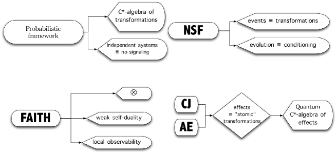
Figure 6. Operational axiomatic framework for quantum Mechanics: summary of the relevant logical implications.

5.4. Reconstructing Quantum Mechanics from the probabilistic theory

It is now possible to reconstruct from the probability tables of the systems the full C^∗-algebra of complex effects ${\mathfrak{E}}_{\mathbb{C}}$ as an operator algebra ${\mathfrak{E}}_{\mathbb{C}}\subseteq\oplus_{i}{\sf Lin(H_{i})}$. Here is the recipe:

1. Look for all sub-cones $({\mathfrak{E}}_{+})_{i}$ invariant under ${\mathfrak{T}}_{+}$.

2. Then, for each $i$:

3. introduce a complex Hilbert space ${\sf H}_{i}$ such that $({\mathfrak{E}}_{\mathbb{C}})_{i}\subseteq{\sf Lin(H_{i})}$, i.e. with $\dim({\sf H}_{i})=\left\lceil\sqrt{\dim[({\mathfrak{E}}_{\mathbb{C}})_{i}]}\right\rceil$, $\lceil x\rceil$ the smallest integer greater than $x$;

4. represent $e$ as the identity over $\oplus_{i}{\sf H}_{i}$;

5. build $({\mathfrak{T}}_{\mathbb{C}})_{i}\subseteq{\sf Lin({\sf Lin({\sf H}_{i})})}$;

6. look for atomic transformations ${\sf Erays}({\mathfrak{T}}_{+})_{i}$;

7. for a given atomic transformation $\mathscr{A}\in{\sf Erays}({\mathfrak{T}}_{+})_{i}$ take an operator $A\in{\sf Lin(H_{i})}$ to represent $\mathscr{A}$ as $A^{\dagger}\cdot A\in{\sf Lin({\sf Lin({\sf H}_{i})})}$;

8. represent $[\mathscr{A}]_{\rm eff}$ as $A^{\dagger}A$;

9. repeat steps 6 and 7 for another transformation $\mathscr{B}$;

10. compose $\mathscr{C}=\mathscr{B}\circ\mathscr{A}$ and represent $\mathscr{C}$ as $C^{\dagger}\cdot C$, with $C=AB$;

11. repeat steps 8 and 9 up to build the whole algebra of effects, and the corresponding representation of the algebra of transformations;

12. construct states as density operators using the Gleason-like theorem [41] for effects [42, 43].

Symbol(s)	Meaning	Related quantities
${\sf S}_{1}\odot{\sf S}_{2}$	Bipartite system obtained by composting ${\sf S}_{1}$ with ${\sf S}_{2}$
${\sf S}=\{\mathbb{A},\mathbb{B},\mathbb{C},\ldots\}$	System
$\mathbb{A},\mathbb{B},\mathbb{C},\ldots$	Tests	$\mathbb{A}=\{\mathscr{A}_{j}\}$ Test$:=$ set of possible events
$\mathscr{A},\mathscr{B},\mathscr{C},\ldots$	Events$\equiv$transformations
$\omega$	states, ${\mathfrak{S}}$ Convex set of states	$\omega(\mathscr{A})$: probability that event $\mathscr{A}$ occurs in state $\omega$
${\mathfrak{T}}$	Convex monoid of transformations/events	${\mathfrak{T}}_{\mathbb{R}}$, ${\mathfrak{T}}_{\mathbb{C}}$: linear spans of ${\mathfrak{T}}$, ${\mathfrak{T}}_{+}$: convex cone
$[\mathscr{A}]_{\rm eff}$	Effect containing event $\mathscr{A}$
$a,b,c,\ldots$	Effects	$e$: deterministic effect
${\mathfrak{E}}$	Convex set of effects	${\mathfrak{E}}_{\mathbb{R}}$, ${\mathfrak{E}}_{\mathbb{C}}$: linear spans of ${\mathfrak{E}}$, ${\mathfrak{E}}_{+}$: convex cone
$\mathbb{L}=\{l_{j}\}$	observable	$\sum_{l_{i}\in\mathbb{L}}l_{i}=e$
${\mathfrak{T}}_{\mathbb{C}}$	C∗-algebra of transformations/events
$a\circ\mathscr{T}$	Operation of transformation $\mathscr{T}$ over effect $a$
$\omega_{\mathscr{A}}$	Conditioned states	$\omega_{\mathscr{A}}:=\omega(\cdot\circ\mathscr{A})/\omega(\mathscr{A}),\qquad$ $\mathscr{A}\omega=\omega(\cdot\circ\mathscr{A})$
${\sf Lin}_{+}({\mathfrak{E}}_{\mathbb{C}})$	Cone of linear maps corresponding to positive bilinear forms over ${\mathfrak{E}}_{\mathbb{C}}$	${\sf Lin}_{+}({\mathfrak{E}}_{\mathbb{C}})=$ $\left\{\mathscr{T}\in{\mathfrak{T}}_{\mathbb{C}}:(a,a\circ\mathscr{T})\geqslant 0,\qquad\right.$ $\left.\forall a\in{\mathfrak{E}}_{\mathbb{C}}\right\}$

Table 1. Summary of notation

6. Conclusions

Theoretical physics should be, in essence, a mathematical “representation” of reality. By “representation” we mean to describe one thing by means of another, to connect the object that we want to understand—the thing-in-itself—with an object that we already know well—the standard. In theoretical physics we lay down morphisms from structures of reality to corresponding mathematical structures: groups, algebras, vector spaces, etc., each mathematical structure capturing a different side of reality.

QM somehow goes differently. We have a beautiful simple mathematical structure—Hilbert spaces and operator algebras—with unprecedented predictive power in the entire physical domain. However, we don’t have morphisms from the operational structure of reality into a mathematical structure. In this sense we can say that QM is not yet truly a “representation” of reality. The large part of the formal structure of QM is a set of formal tools for describing the process of gathering information in any experiment, independently of the particular physics involved. It is mainly a kind of information theory, a theory about our knowledge of physical entities rather than about the entities themselves. If we strip off such informational part from the theory, what would be left should be the true general principle from which QM should be derived.

In the present work I have analyzed the possibility of deriving QM as the mathematical representation of a fair operational framework made of a set of rules which allows one to make predictions on future events on the basis of suitable tests. The two Postulates NSF and PFAITH need to be satisfied by an operational framework that is fair, the former in order to be able to make predictions based on present tests, the latter to allow calibrability of any test and preparability of any state. We have seen that all theories satisfying NSF admit a C^∗-algebra representation of events as linear transformations of complex effects. Based on a very general notion of dynamical independence, all such theories are non-signaling. The C^∗-algebra representation of events is just the informational part of the theory. We have then added Postulate PFAITH. Postulate PFAITH has been proved to be remarkably powerful, implying the local observability principle, the tensor-product structure for the linear spaces of states and effects, weak self-duality, and a list of features such as realization of all states as transformations of the marginal faithful state $\Phi(e,\cdot)$, locally indistinguishable ensembles of states corresponding to local observables—i.e. impossibility of bit commitment, and more. We have then explored a postulate dual to PFAITH, Postulate FAITHE for effects, thus deriving additional quantum features, such as teleportation. We feel that we are really close to QM: maybe we are already there and we only need to prove it! All the consequences of these postulates need to be explored further. I have also reported some consequences of a postulate about the purifiability of all states. In any case, we have seen that whichever is the missing postulate, it must establish a one-to-one correspondence between complex effects and atomic transformations, which, assuming atomicity of evolution (Postulate AE) will make also effects a C^∗-algebra. This is what is special about QM (and all hybrid quantum-classical theories), and will exclude the other non-signaling probabilistic theories of the kind of the PR-boxes. We have seen that the correspondence between effects and atomic transformations is established by the Choi-Jamiolkowski isomorphism, which is hoped to be not too far from an operational principle.

References

- [1] G. Birkhoff and J. von Neumann, The logic of quantum mechanics, Ann. Math. 37 823 (1936).
- [2] P. Jordan, J. von Neumann, and E. Wigner, On an algebraic generalization of the quantum mechanical formalism, Ann. Math. 35 29 (1934).
- [3] V. S. Varadarajan, Probability in physics and a theorem on simultaneous observability, Comm. Pure and Appl. Math. 15 189 (1962).
- [4] G. W. Mackey, Mathematical Foundations of Quantum Mechanics (Benjamin, New York, 1963).
- [5] C. Piron, Foundations of Quantum Physics (Benjamin, Massachusets, 1976).
- [6] I. E. Segal, Postulates for general uantum mechanics, Ann. Math. 48 930 (1947).
- [7] F. Strocchi, An introduction to the mathematical structure of quantum mechanics: A short course for mathematicians, Advanced Series in Mathmatical Physics (World Scientific, Singapore, 2005).
- [8] E. M Alfsen and F. W Shultz, State spaces of operator algebras: Basic theory, orientations, and C*-products, Mathematics: Theory and Applications (Birkha̋user, Boston, 2001).
- [9] E. M Alfsen and F. W Shultz, Geometry of state spaces of operator algebras, Mathematics: Theory and Applications (Birkha̋user, Boston, 2002).
- [10] W. Thirring, Quantum mathematical physics (Springer, Berlin, 2004).
- [11] G. Ludwig, An axiomatic basis for quantum mechanics i: Derivation of Hilbert space structure (Springer, Berlin, 1985).
- [12] L. Hardy, Quantum theory from five reasonable axioms, quant-ph/0101012v4 (2001).
- [13] R. Clifton, J. Bub, and H. Halvorson, Characterizing quantum theory in terms of information-theoretic constraints, Found. Phys. 33 1561 (2003).
- [14] G. M. D’Ariano, Operational axioms for quantum mechanics, in Foundations of Probability and Physics-4, ed. by G. Adenier, C. A. Fuchs, and A. Y. Khrennikov, CP889 (AIP, Melville, New York, 2007) pag.79
- [15] G. M. D’Ariano, On the missing axiom of quantum mechanics, Quantum Theory, Reconsideration of Foundations - 3, Va̋xjő, Sweden, 6-11 June 2005 (Melville, New York) (G. Adenier, A. Y. Khrennikov, and T. M. Nieuwenhuizen, eds.), (AIP, Melville, New York 2006) pp. 114.
- [16] G. M. D’Ariano, How to derive the Hilbert-space formulation of quantum mechanics from purely operational axioms, in Quantum Mechanics, ed. by A. Bassi, D. Duerr, T. Weber and N. Zanghi, AIP CP844 (AIP, Melville, New York, 2006) p. 101.
- [17] G. M. D’Ariano, Operational axioms for c*-algebra representation of transformations, in Quantum Theory, Reconsideration of Foundations 4, ed. by G. Adenier, A. Yu Khrennikov, P. Lahti, V. I. Man’ko, and Th. M. Nieuwenhuizen, CP962 (AIP, Melville, New York, 2007) p. 44.
- [18] G. M. D’Ariano, Operational axioms for a c*-algebraic formulation for quantum mechanics, in Proceedings of the 8th Int. Conf. on Quantum Communication, Measurement and Computing, ed. by O. Hirota, J. H. Shapiro and M. Sasaki (NICT press, Japan, 2007), p. 345
- [19] G. M. D’Ariano, Where the mathematical structure of quantum mechanics comes from, in Beyond the Quantum, ed. by T. M. Nieuwenhuizen, V. Spicka, B. Mehmani, M. J. Aghdami, A. Y. Khrennikov (World Scientific, Singapore, 2007) pag. 191
- [20] S. Popescu and D. Rohrlich, Quantum nonlocality as an axiom, Found. Phys. 24 379 (1994).
- [21] B. S. Cirel’son, Quantum generalizations of bell’s inequality, Lett. Math. Phys. 4 93 (1980).
- [22] C. Simon, V. Bužek, and N. Gisin, No-signaling condition and quantum dynamics, Phys. Rev. Lett. 87 170405 (2001).
- [23] H. Barnum, J. Barrett, M. Leifer, and A. Wilce, Generalized no-broadcasting theorem, Phys. Rev. Lett. 99 240501 (2007).
- [24] J. Barrett, Information processing in generalized probabilistic theories, quant-ph/0508211 (2005).
- [25] H Barnum, J Barrett, M Leifer, and A Wilce, Teleportation in general probabilistic theories, quant-ph/0805.3553 (2008).
- [26] H. Barnum, Coordinating quantum agents’ perspectives: convex operational theories, quantum information, and quantum foundations, quant-ph/0611110 (2006).
- [27] M.-D. Choi, Completely positive linear maps on complex matrices, Lin. Alg. Appl. 10 285 (1975).
- [28] A. Jamiolkowski, Linear transformations which preserve trace and positive semidefiteness of operators, Rep. Math. Phys. 3 275 (1972).
- [29] A. Rényi, Foundations of Probability (Dover, Mineola, N. Y. 2007)
- [30] G. Chiribella, G. M. D’ariano, and P. Perinotti, Quantum circuit architecture, Phys. Rev. Lett. 101 060401 (2008).
- [31] G. Chiribella, G. M. D’ariano, and P. Perinotti, Operational axioms for the dilation of physical processes (in preparation).
- [32] A. Barvinok, A Course in Convexity (American Mathematical Society, Providence, 2002).
- [33] J. Béllissard and B. Iochum, Homogeneous self-dual cones, versus jordan algebras. The theory revisited, Ann. Inst. Fourier (Grenoble) 28 27 (1978).
- [34] C. A. Fuchs, Quantum Mechanics as Quantum Information (and only a little more), quant-ph/0205039 (2002).
- [35] D. Koehler and P. Rosenthal, On isometries of normed linear spaces, St. Math. 36 213 (1970).
- [36] G. M. D’Ariano, No-signalling, dynamical independence and the local observability principle, J. Phys. A: Math. Theor. 40 8137 (2006).
- [37] V B Scholz and R F Werner, Tsirelson’s Problem, arXiv 0812.4305 (2008).
- [38] G. M. D’Ariano, D. Kretschmann, D. Schlingemann, and R. F. Werner, Reexamination of quantum bit commitment: The possible and the impossible, Phys. Rev. A 76 (2007) 27.
- [39] R. Haag, Local quantum physics: Fields, particles, algebras (Springer, Berlin, 1996).
- [40] I. M. Gelfand and M. A. Neumark, On the imbedding of normed rings into the ring of operators in Hilbert space, Mat. Sb. 12 197 (1943).
- [41] A. M. Gleason, Measures on the closed subspaces of a Hilbert space, J. Math. Mech. 6 885 (1957).
- [42] P Busch, Quantum states and generalized observables: A simple proof of gleason’s theorem, Phys. Rev. Lett. 91 120403 (2003).
- [43] C. M. Caves, C. A. Fuchs, K. Manne, and J. Renes, Gleason’s theorem with POVMS (unpublished, 2000).
- [44] A. J. Short, S. Popescu, and N. Gisin, Entanglement swapping for generalized nonlocal correlations, Phys. Rev. A 73 012101 (2006).