Recent OH Zeeman Observations:
Do they Really Contradict the Ambipolar-Diffusion Theory of Star Formation?

Abstract

Until recently, many of the dozens of quantitative predictions of the ambipolar-diffusion theory of gravitational fragmentation (or core formation) of molecular clouds have been confirmed by observations and, just as importantly, no prediction has been contradicted by any observation. A recent paper, however, claims that measurements of the variation of the mass-to-flux ratio from envelopes to cores in four clouds decreases, in direct contrast to a prediction of the theory but in agreement with turbulent fragmentation (in the absence of gravity) and, therefore, the ambipolar-diffusion theory is invalid (Crutcher et al. 2008). The paper treats magnetic-field nondetections as if they were detections. We show that the analysis of the data is fundamentally flawed and, moreover, the comparison with the theoretical prediction ignores major geometrical effects, suggested by the data themselves if taken at face value. The magnetic fluxes of the envelopes are also miscalculated. We carry out a proper error analysis and treatment of the nondetections and we show that the claimed measurement of the variation of the mass-to-flux ratio from envelopes to cores is not valid, no contradiction with the ambipolar-diffusion theory can be concluded, and no theory can be tested on the basis of these data.

1. Introduction

The ratio of the mass and magnetic flux of interstellar molecular clouds has received well-deserved observational attention in recent years (e.g., Crutcher 1999; Heiles & Cructher 2005). For a cloud as a whole, the mass-to-flux ratio is important input to the ambipolar-diffusion theory of fragmentation (or core formation) in molecular clouds. For fragments (or cores) within a cloud, the ambipolar-diffusion theory makes specific predictions of the mass-to-flux ratio and its evolution in time. Until now, observations have been in excellent quantitative agreement with the theoretical predictions (e.g., see Crutcher et al. 1994; Crutcher 1999 and correction by Shu et al. 1999, pp. 196 - 198; Ciolek & Basu 2000). Recently, however, Crutcher et al. (2008) (hereinafter CHT) have looked at the variation of the mass-to-flux ratio from the envelopes to the cores of four molecular clouds and concluded that there is a fundamental discrepancy between the observations and the predictions of the ambipolar-diffusion theory.

In what follows, we examine critically the claimed discrepancy. Before we undertake a direct re-examination of the data and the conclusions drawn from them, it is important that we summarize the key elements of the ambipolar-diffusion theory of protostar formation. This is especially necessary because, often, what is a prediction of the theory is quoted as if it were a requirement or assumption, and vice versa, i.e., input of the theory taken directly from observations is often quoted as if it were a prediction. The ambipolar-diffusion timescale is also often a frequent victim of abuse in the astronomical literature. In this context, it is of utmost importance to clarify the difference in the way the process of ambipolar diffusion affects the ordered (or mean) component of the magnetic field in a molecular cloud and the magnetohydrodynamic (MHD) waves (or turbulence) that are superimposed on the mean field. It is also useful, for putting the current controversy in its proper context and perspective, to summarize how theory and observations of interstellar magnetic fields have interacted over the years and what the outcome of that interaction has been.

We summarize in §2.1 the main elements of the ambipolar-diffusion theory in a context relevant to the present controversy and to maintaining proper perspective. In §2.2 we first summarize the observational procedure followed by CHT and state their main conclusion, and then we state three major flaws in their analysis as well as three additional such flaws in their comparison of the results with the ambipolar-diffusion theory.

In §3, we explain the proper procedure for combining multiple observations of the envelope magnetic field in each cloud to derive an estimate of the mean and an associated uncertainty. An explicit assumption of the analysis by CHT is that line-of-sight effects (as encoded in $\cos\theta$) are the same for the core and the envelope. An implicit assumption of the same analysis is that the magnetic field does not vary intrinsically from one envelope location to another. None of these assumptions is justified by the observations. Relaxing them in a manner suggested by the data themselves alters the manner in which errors should be treated and increases significantly the uncertainties of all results.

In §4, we discuss the difference between a detection and an upper limit of the mean envelope magnetic field. Most of the individual observations yielded nondetections, a fact recognized by the authors. The authors state that for this experiment detections are not necessary. No upper limits are calculated, which would be appropriate for nondetections; instead, nondetections and detections are treated in the same way with respect to error propagation and handling, as well as for quoting results. We remedy this problem and explicitly calculate upper limits where appropriate, using a full Monte Carlo analysis of the error propagation to properly account for the (large) errors propagating through a nonlinear equation (see eq. [7] below).

In §5, we elaborate certain theoretical issues (points 3a, b, c of §2.2) which should be paid due consideration if a meaningful comparison between theory and observations is to be achieved at least as far as the variation of the mass-to-flux ratio from the envelope to the core of a molecular cloud is concerned.

2. The Development of the Ambipolar-Diffusion Theory, its Main Elements, and Recent OH Zeeman Observations

2.1. Key Elements of the Ambipolar-Diffusion Theory of Protostar Formation

Ambipolar diffusion (the motion of the two poles of charge, ions and electrons and possibly charged grains, which at densities characteristic of molecular clouds are well attached to magnetic field lines, relative to the neutral particles) is an unavoidable process in weakly ionized, self-gravitating systems, e.g., molecular clouds. It occurs on a timescale given by (see Mouschovias 1979b)

$$\tau_{\rm AD}=1.8\times 10^{6}\,\left(\frac{x_{\rm i}}{10^{-7}}\right)\,\,\,{\rm yr},$$ (1)

where $x_{\rm i}$ is the degree of ionization. Unlike the early understanding of this process, which envisioned magnetic flux escaping a cloud as a whole and thereby depriving a cloud of magnetic support and allowing it to collapse and form stars (e.g., Mestel & Spitzer 1956; Nakano & Tademaru 1972; Nakano 1973, 1976, 1977), a re-examination of the process concluded that ambipolar diffusion is much more effective in the deep interiors of molecular clouds, where the degree of ionization is smaller than $10^{-7}$, than in their envelopes, where the degree of ionization is usually greater or much greater than $10^{-5}$. The important difference in the two pictures is that, in the latter, a cloud as a whole does not lose any magnetic flux. Instead, neutral particles, under their own self-gravity, contract slightly more rapidly than the plasma (and the field lines), thereby redistributing the mass in the central parts of a dense cloud and increasing the mass-to-flux ratio in the central flux tubes (but not necessarily in an individual fragment or core; see below).

Early efforts to understand the possible role of ambipolar diffusion in cloud dynamics and star formation consisted almost exclusively of comparing $\tau_{\rm AD}$ (actually, an earlier version of this timescale obtained by Spitzer 1968 for uniform, cylindrical cloud models and which was greater than that given by eq. [1] by almost a factor of 3) and the free-fall time, which for a spherical cloud model of uniform neutral density $\rho_{\rm n}$ is given by

$$\tau_{\rm ff}=\left(\frac{3\pi}{32G\rho_{\rm n}}\right)^{1/2}\,=1.07\times 10^{6}\,{\left(\frac{10^{3}\,{\rm cm^{-3}}}{n_{\rm n}}\right)}^{1/2}\,\,\,{\rm yr}.$$ (2)

Since $\tau_{\rm AD}$ was invariably found to be greater than $\tau_{\rm ff}$, it was always concluded that ambipolar diffusion is not a relevant process in star formation. The presumption was that a cloud gives birth to stars on the free-fall timescale, as orginally suggested by Hoyle in his hierarchical fragmentation picture, or on a somewhat longer (”‘magnetically diluted”) free-fall time because of the presence of a magnetic field frozen in the matter (Mestel 1965).

A series of papers initiated and developed the main elements of the modern theory of single-stage fragmentation (or, core formation) and star formation in molecular clouds as a natural consequence of primarily magnetic support of such clouds (Mouschovias 1977, 1978, 1979, 1981, 1987a,b, 1989, 1991a, b, c; Shu et al. 1987). Observations were already suggesting that star formation does not occur on the free-fall timescale but on a timescale exceeding $10^{7}$ yr (e.g., see Roberts 1969; Zuckerman & Palmer 1974). Magnetic support was neither an arbitrary theoretical assumption nor an ingenious theoretical conclusion. It was a simple consequence of the fact that the then observed interstellar, large-scale magnetic field of 3 $\mu$G can easily support a mass of $5\times 10^{5}\,{\rm M_{\odot}}$ at the approximate mean density of the interstellar medium of $1\,{\rm cm^{-3}}$. Moreover, atomic-hydrogen clouds, thought to be the progenitors of molecular clouds have never been observed to have mass-to-flux ratios exceeding the critical value for collapse

$$\left(\frac{M}{\Phi_{B}}\right)_{\rm crit}=\left(\frac{1}{63G}\right)^{1/2},$$ (3)

obtained from nonlinear, exact equilibrium calculations (Mouschovias & Spitzer 1976). (The quantity $G$ is the universal gravitational constant.) In addition, if clouds were to begin their lifetimes in a magnetically supercritical state, contraction (ordered) velocities characteristic of collapse (several ${\rm km\,s^{-1}}$) would be commonplace. Instead, the gravitational potential energy of typical HI clouds is smaller than their magnetic energy by two orders of magnitude, and velocities characteristic of collapse for a cloud as a whole are not observed even for molecular clouds.

Mouschovias (1987a) described a new theory of star formation in primarily magnetically supported molecular clouds, with hydromagnetic waves (or turbulence) contributing part of the support against gravity. (At the time, it was referred to as a “scenario” because the rigorous, quantitative calculations needed to justify the term “theory”, which implies predictive power, had not yet been undertaken.) Ambipolar diffusion, which as explained above is an unavoidable process in a weakly ionized, self-gravitating physical system such as a molecular cloud, acts differently on the large-scale (or mean) magnetic field and on short-wavelength disturbances associated with MHD waves or turbulence. Because of ambipolar diffusion, disturbances of wavelength $\lambda$ smaller than the Alfvén lengthscale

$$\lambda_{\rm A}=\pi v_{\rm A}\tau_{\rm ni}$$ (4)

cannot be sustained in the neutrals; i.e., they decay because of neutral-ion friction. (The quantity $v_{\rm A}=B/(4\pi\rho_{\rm n})^{1/2}$ is the Alfvén speed in the neutrals, and $\tau_{\rm ni}$ the mean (elastic) collision time of a neutral particle in a sea of ions.) Unlike the timescale for redistribution of mass in the central flux tube of a cloud given by equation (1), the timescale for the decay of such disturbances is wavelength ($\lambda$) dependent and is given by

$$\tau_{\rm{AD,wave}}\approx 10^{5}\left(\frac{\lambda}{\rm{1\,pc}}\right)^{2}\!\!\!\left(\frac{30\,\mu\rm{G}}{B}\right)^{2}\!\!\!\left(\frac{n_{\rm{n}}}{10^{3}\,{\rm cm^{-3}}}\right)\!\!\!\left(\frac{x_{\rm i}}{10^{-7}}\right)\,\,\,{\rm yr}.$$ (5)

This is a very short timescale even relative to free-fall, and it becomes smaller the smaller the wavelengths one considers. For typical molecular-cloud parameters, the Alfvén lengthscale is arithmetically equal (0.3 pc) to the thermal critical lengthscale (essentially the Bonnor-Ebert radius for collapse of an isothermal sphere supported by thermal pressure against its self-gravity),

$$\lambda_{\rm{T,crit}}=1.09C_{\rm a}\tau_{\rm ff}=0.29\left(\frac{T}{10\,\rm{K}}\right)^{1/2}\!\!\!\left(\frac{10^{3}\,{\rm cm^{-3}}}{n_{\rm n}}\right)^{1/2}\,\,\,{\rm pc},$$ (6)

where $C_{\rm a}$ is the adiabatic speed of sound in the gas. Thus, if MHD waves (or turbulence) contribute even a small fraction of the support against gravity (e.g., a few percent), ambipolar diffusion removes that support very quickly and gravity remains locally unbalanced. Ambipolar diffusion, then, allows thermally supercritical but magnetically subcritical masses to begin to separate out as fragments (or cores). Eventually, the mass-to-flux ratio of the central flux tube of a cloud exceeds the critical value for collapse and dynamical contraction (but not free fall) ensues. This was the conceptual origin of the new theory of fragmentation and star formation suggested by Mouschovias (1987a; see also 1991a) and put on a rigorous footing in subsequent years (e.g., see review by Mouschovias 1996 and references therein).

Statements frequently encountered in the literature, to the effect that the ambipolar-diffusion theory ignores MHD waves (or turbulence), are thus not based on the record. It is precisely because of the partial support that such disturbances provide against gravity and their consequent decay by ambipolar diffusion that fragmentation (or core formation) is initiated in this theory. It is noteworthy that, the greater the initial contribution of such disturbances to the support against gravity, the more rapid the ambipolar-diffusion–initiated fragmentation process becomes.

An important prediction of the detailed numerical simulations was that the central mass-to-flux ratio, after it exceeds the critical value given by equation (3) and dynamical contraction (but not free fall) sets in, does not continue to increase indefinitely. It asymptotes to a value typically 2 - 3 times greater than the critical one (e.g., Fiedler & Mouschovias 1993, Fig. 9b; Ciolek & Mouschovias 1994, Figs. 2e and 4e). The physical reason for this is that the contraction is rapid (the infall acceleration is typically 30% that of gravity), so that the magnetic flux is essentially trapped inside the contracting fragment. Once such gravitational contraction begins, unlike the early, ambipolar-diffusion–controlled phase of core formation in which the magnitude of the magnetic field does not typically increase by more than 30%, the magnetic field increases with gas density as $B\propto\rho^{\kappa}$ with $\kappa\approx 1/2$.

Critics of the ambipolar-diffusion theory often refer to the large set of calculations that developed and refined the theory as “static”. Far from that being the case, these calculations have demonstrated that, even if one begins with a model cloud that is in an initial exact equilibrium state and would therefore remain in such a state indefinitely if it were not for the presence of ambipolar diffusion, the fragmentation is relatively rapid (more precisely, it occurs on a timescale equal to 1/2 the value given by eq. [1]) and, moreover, these calculations are the only ones that have followed the subsequent dynamical phase of protostar formation, up to densities of about $10^{15}\,{\rm cm^{-3}}$, accounting for the zoo of phenomena relevant to the seven-fluid physical system (neutral particles, atomic and molecular ions, electrons, negatively-charged, positively-charged and neutral grains) – e.g., see Tassis and Mouschovias (2007a, b, c). Mindful of the possibility that molecular clouds are not quiescent objects and are not necessarily found in quiescent environments, Mouschovias (1987a, fig. on p. 486; or 1991a, Fig. 1) considered both subAlfvénic as well as superAlfvénic contraction. Yet in both cases, ambipolar diffusion (and magnetic braking) plays a crucial role in protostar formation.

It was recognized early on in the development of the ambipolar-diffusion theory of fragmentation that, once a flux tube in a molecular cloud becomes magnetically supercritical, it may break up along its length into thermally supercritical but magnetically subcritical fragments (Mouschovias 1991c, §2.4). In fact, the factor by which the density of such fragments must increase in order for balance of forces along field lines to be re-established and a critical mass-to-flux ratio to be re-acquired was calculated analytically. Moreover, the effect that such fragmentation has on the $B-\rho$ relation was also determined. It is therefore of utmost importance to keep in mind these effects if one desires to make a statement about the mass-to-flux ratio of a single fragment relative to that of the parent cloud. In other words, if a magnetically critical or supercritical flux tube breaks up along its length, the entire mass in the flux tube must be counted if one desires to obtain the relevant mass-to-flux ratio to compare with the theoretical prediction.

The theory has three significant dimensionless free parameters, whose typical values are obtained from observations (Fiedler & Mouschovias 1992). Accounting for rotation introduces a fourth free parameter, which is essentially a measure of the moment of inertia of the cloud (or fragment) relative to that of a region in the surrounding medium (or envelope) of volume comparable to that of the cloud (or fragment) (Basu & Mouschovias 1994). A simulation is carried out using those typical values of the free parameters as input. The calculation predicts the spatial dependence and time evolution of the physical quantities of the forming protostellar fragment and of the parent cloud (e.g., profiles of the density, magnetic field, angular velocity, infall velocity as functions of time). In the calculations without rotation, the three free parameters are: (1) the initial central mass-to-flux ratio $\mu_{\rm c0}$ in units of its critical value for collape; (2) the ratio of the initial free-fall time and the neutral-ion collision time, $\nu_{\rm{}ff,0}$; and (3) the exponent $k$ in the parametrization of the ion density $n_{\rm i}$ in terms of the neutral density $n_{\rm n}$, $k=d{\rm ln}{n_{\rm i}}/d{\rm ln}{n_{\rm n}}$. If detailed grain chemistry is used to determine the degree of ionization at each stage of the evolution, the parameter $k$ is replaced by a quantity which is essentially the radius of a typical grain particle (Ciolek & Mouschovias 1993). Once the results from the fiducial run are at hand, a parameter study is carried out. It consists of at least two additional runs for each of the free parameters, using values at the endpoints of the range suggested or allowed by observational uncertainties. Since the mass-to-flux ratio of the parent cloud (or envelope) is a dimensionless free parameter in the theory, the theory neither requires nor predicts that this quantity have any specific value, e.g., be subcritical. The fact that, in any cloud in which a positive detection of the magnetic field component along the line of sight using Zeeman observations has been obtained, implies that the cloud’s mass-to-flux ratio (given the geometrical uncertainties in estimating it) is consistent with a subcritical value is just that, observational input to the theory, not a requirement or a prediction of the theory.

Early observational work using the Zeeman effect in the 21-cm line of HI, focused on testing the relation between the magnetic field strength and the gas density predicted by spherical, isotropic contraction, i.e., $B\propto\rho^{2/3}$ (e.g., Verschuur 1970, 1971). It was concluded that the observations were consistent with that relation. However, a more careful examination of the data showed that that was not the case (Mouschovias 1978, Fig. 1). Instead, the data was consistent with the prediction of the early, self-consistent calculations of the equilibrium and contraction of self-gravitating, isothermal, magnetic clouds embedded in a hot and tenuous external medium. Subsequent observations of the Zeeman effect in OH (which samples greater densities than HI) and in OH and $\rm{H_{2}O}$ masers (which sample even greater densities and reveal physical conditions in regions of active star formation) were found to be as predicted by the magnetic calculations (Fiebig & Guesten 1989; Mouschovias 1996, Fig. 1b; Crutcher 1999).

More recently, observational attention has shifted from the $B-\rho$ relation to the mass-to-flux ratio, which, for a cloud as a whole is invaluable input to the ambipolar diffusion theory and, for fragments (or cores) can potentially be an important test of the theoretical prediction that ambipolar diffusion leads to an increase of the mass-to-flux ratio of a cloud’s central flux tubes relative to the mass-to-flux ratio of the envelope.

2.2. Recent OH Zeeman Observations

CHT have recently combined existing detections of the OH Zeeman effect in four molecular cloud cores with new observations of the same effect in the regions surrounding these cores, in an effort to get a handle on the variation of the mass-to-flux ratio from the envelope to the core of each cloud. The authors regard this as a definitive test of the ambipolar diffusion theory. The four clouds are L1448, B217-2, L1544, and B1. In the region surrounding each core in each of the four clouds, new observations were undertaken at four locations about each core (i.e., in the envelope of each core). At some locations in each envelope, positive detections were made while at others no detection could be achieved. For each envelope, the authors average the algebraic values of the four measurements of the line-of-sight magnetic field, regardless of whether they were detections or nondetections, and assign the resulting value to the average magnetic field strength of the envelope – the assumption made here is that this value appropriately characterizes the mean magnetic field of the envelope. Using this field, CHT proceed to calculate what they regard as the magnetic flux of the envelope, which, combined with the flux in the core, is used to obtain the quantity $R$ defined by

$$R=\frac{I_{\rm core}\Delta V_{\rm core}/{B_{\rm core}}}{I_{\rm env}\Delta V_{\rm env}/{B_{\rm env}}}.$$ (7)

(The quantity $I$ is the peak intensity of the spectral line in degrees K, $\Delta V$ is the FWHM in km $\rm s^{-1}$, and $B$ is the line-of-sight magnetic field strength in microgauss.) They then average again the values of $R$ over the four clouds, and obtain an overall average value of $R$. The claim in the paper is that the derived value of $R$ is 5$\sigma$ away from 1 and that this contradicts a prediction of the ambipolar diffusion theory and, therefore, invalidates the theory, since the latter (according to CHT) predicts $R>1$.

We show quantitatively below that this claim, as stated by CHT, is not supported by their data; it is an artifact of the analysis and interpretation of the data, which suffers in three major ways:

1. The treatment of the propagation of observational uncertainties systematically underestimates the uncertainties of the combined result at every step.

2. Nondetections of magnetic fields are treated as if they were detections, and upper limits are not quoted as appropriate – in fact, based on the raw data presented in CHT, measurements of $R$ are not achievable in any of the clouds studied; rather, upper limits should have been calculated and quoted.

3. The comparison with ambipolar-diffusion calculations is itself flawed in three important respects:

(a) The theoretical simulations chosen for this comparison use as input a very different geometry of the field lines threading the cloud from the geometry of the field lines that the observations presumably reveal.

(b) The magnetic flux threading each cloud is incorrectly calculated by taking the arithmetic average of the four algebraic values of $B$ in each envelope.

(c) The possible breakup of the mass in the central flux tube of each cloud into thermally supercritical but magnetically subcritical fragments (or cores), an important possible effect in the theory (Mouschovias 1991c), is mentioned by the authors but not taken into consideration in their analysis and/or arguments.

If these effects are considered, it follows that a variety of $R-$values are possible. We discuss each of these points below.

3. Combining Uncertainties and Propagating Errors

CHT quote values for the results of observations of the magnetic field at four different positions in the envelope of each cloud, together with associated uncertainties, derived as in Troland & Crutcher (2008). In most cases, the quoted values correspond to nondetections. We discuss this issue in detail in the next section; here, we refer to detections and nondetections alike as “observations”.

For each observation of the envelope’s line-of-sight magnetic field $B_{j}$, CHT quote an associated uncertainty $\sigma_{j}$, which we assume to be Gaussian. These values are given for each cloud in Table 1. The authors then calculate a mean value of the line-of-sight magnetic field in the envelope of each cloud,

$$B_{\rm mean}=\frac{1}{4}\sum_{j=1}^{4}B_{j}\,,$$ (8)

and an uncertainty on the mean, $\sigma_{\rm mean}$, using Gauss’ formula of error propagation on equation (8), which gives

$$\sigma_{\rm mean}=\frac{1}{4}\sqrt{\sum_{j=1}^{4}\sigma_{j}^{2}}\,.$$ (9)

The results derived using this formula are given in the second column of Table 2; they are the same as those quoted in CHT (see their Table 1, col. 4).

Table 1 Magnetic Fields and Errors (in microgauss) in Four Cloud Envelopes (data from CHT).

Cloud	$B_{1}\pm\sigma_{1}$	$B_{2}\pm\sigma_{2}$	$B_{3}\pm\sigma_{3}$	$B_{4}\pm\sigma_{4}$
L1448CO	$-9\pm 13$	$-11\pm 6$	$-7\pm 7$	$14\pm 8$
B217-2	$-13\pm 9$	$5\pm 6$	$6\pm 8$	$9\pm 13$
L1544	$-3\pm 4$	$-1\pm 4$	$22\pm 6$	$2\pm 10$
B1	$-16\pm 6$	$0\pm 7$	$-3\pm 6$	$-10\pm 5$

This analysis is a standard treatment of errors when combining several measurements of the same quantity. If CHT had mesured the magnetic field at the same envelope location in four different instances, their measurements could be combined using this procedure (although, even in this case, a weighted average and its associated error propagation formula would be more appropriate since the measurement uncertainties are not equal for every observation). Similarly, if there were an a priori reason to be certain that the envelope magnetic field is uniform and the four observations in each cloud are sampling the same value of the field, such treatment would be appropriate. However, this is not the case here, and the treatment of errors in CHT yields misleading results. We discuss the reasons below.

First, it cannot be overemphasized that Gauss’ formula for error propagation, and hence equation (9), is not universally applicable. There are two reasons for which applicability might fail. The first stems from the fact that Gauss’ formula is based on a Taylor expansion (e.g., see, Wall & Jenkins 2003). As such, it is valid only if the errors being propagated are small, or if the equation through which the errors are propagated is linear (and thus no second-order terms enter the calculation). This condition does indeed apply in this case: although the errors are by no means small, the average is a linear operation and no second-order terms enter the error propagation formula. The second reason for which the applicability of Gauss’ formula might fail is if the observations being combined are not measuring the same intrinsic quantity, but rather a distribution of values. Then, one’s ability to constrain the mean, especially in the small-number–statistics regime, is not simply dependent on one’s ability to take individual measurements; the possibility of having finite distribution spreads needs to be explicitly accounted for.

The magnetic field in the cloud envelope is not known a priori to have a unique uniform value everywhere in the envelope. In fact, the data seem to suggest exactly the opposite (e.g., compare observations 1 and 2 in cloud L1544 with observation 3 in the same cloud - see Table 1). Equation (9) is therefore not the appropriate estimate for the uncertainty on the mean magnetic field for each cloud envelope. What should one use instead?

The spread in the observations is the convolution of the observational uncertainty and the intrinsic spread of the distribution of magnetic field values across the envelope. The sample variance can give an estimate of this convolved spread; its square root (the sample standard deviation, an unbiased estimator of the population standard deviation $\sigma$) is given by

$$\sigma_{S}=\sqrt{\frac{1}{3}\sum_{i=1}^{4}\left(B_{j}-B_{\rm mean}\right)^{2}}\,.$$ (10)

It is well known (e.g., see Wall & Jenkins 2003; Lyons 1992) that the average, given by equation (8), is distributed as a Gaussian about the true value of the mean, with variance $\sigma^{2}/N$ where $N$ is the number of observations. In our case, $N=4$ and the standard deviation of the average, which is the uncertainty on the mean, is $\sigma/2$. For all clouds, the best-guess estimate of $\sigma$, which is $\sigma_{S}$, is $\geq$ twice the uncertainty quoted on the mean (note, for example, the case of L1544 where the uncertainty quoted by CHT on the mean is $3{\rm\,\mu G}$ while $\sigma_{S}/2=6{\rm\mu G}$). This is an empirical proof that the uncertainties quoted by CHT are underestimated, even if one were to ignore the conceptual point made above.

Even $\sigma_{S}/2$, however, underestimates the true uncertainty on the mean. The uncertainty on the mean is $\sigma/2$, not $\sigma_{S}/2$. The sample standard deviation $\sigma_{S}^{2}$ is only an estimate of the population variance $\sigma^{2}$, and is distributed as $\sigma^{2}\chi^{2}/(N-1)$, where $\chi^{2}$ is a $\chi$-square variable with $N-1$ degrees of freedom (e.g., see Wall & Jenkins 2003). In practical terms, this means that, in the low-statistics regime we are considering, $\sigma_{S}$ most frequently underestimates $\sigma$, and in about $10\%$ of all instances does so by at least a factor of $2$. In the latter case, the appropriate uncertainty on the mean is closer to $\sigma_{S}$ rather than $\sigma_{S}/2$. How do we then take into account not only that there is a finite population spread, but also that this population spread is essentially unknown, due to our inability to constrain it very well with the very limited number of available observations?

We must use an analysis that allows not only for finite spreads, but also for a variety of such spreads, as long as they are allowed by the data. Allowing for a range of finite spreads consistent with the data increases the range of mean values that can explain the data, and in this way increases the uncertainty on the mean. Conversely, ignoring the possibility that there is true variation of mostly unknown extent of the $B_{\rm los}$ from point to point in the envelope artificially decreases the uncertainty in the mean $B_{\rm los}$ value.

Table 2 Derived mean envelope magnetic fields and uncertainties. Two left columns: CHT treatment; third column: sample standard deviation; fourth column: likelihood analysis results (this work).

Cloud	$B_{\rm mean}\pm\sigma_{\rm mean}$	$\sigma_{S}$	$B_{{\rm max}\mathcal{L}}\pm\sigma_{\mathcal{L}}$
L1448CO	$-3\pm 4$	12	$-4^{+9}_{-8}$
B217-2	$+2\pm 5$	10	$+2^{+7}_{-7}$
L1544	$+5\pm 3$	12	$+4^{+10}_{-8}$
B1	$-7\pm 3$	7	$-8^{+5}_{-5}$

The most straightforward way to correctly combine these observations while allowing for finite spatial spread of $B_{\rm los}$ is through a likelihood analysis (e.g., see Wall & Jenkins 2003; Lyons 1992; Lee 2004). In a likelihood analysis, the data can be assumed to be derived from a parent distribution of values (in our case, we assume that values of $B_{\rm los}$ in the envelope follow a Gaussian distribution with mean equal to $B_{0}$ and intrinsic spread $\sigma_{0}$). This distribution is then “sampled” with $N$ measurements $B_{j}$, each carrying a (Gaussian) uncertainty of measurement $\sigma_{j}$. ¿From the data, we then calculate the joint probability distribution of the parameters $B_{0},\sigma_{0}$ which are consistent with observations (the likelihood). In our case, the likelihood can be shown to be (e.g., see Venters & Pavlidou 2007, and appendix A)

$$\mathcal{L}\left(B_{0},\sigma_{0}\right)=\left(\prod_{j=1}^{N}\frac{1}{\sqrt{\sigma_{0}^{2}+\sigma_{j}^{2}}}\right)\exp\left[-\frac{1}{2}\sum_{j=1}^{N}\frac{(B_{j}-B_{0})^{2}}{\sigma_{0}^{2}+\sigma_{j}^{2}}\right]\,.$$ (11)

Any parameters that are not of direct interest to us (such as $\sigma_{0}$ in our case), can then be integrated out of the likelihood. In this way, we can derive the probability distribution of the parameter of interest ($B_{0}$ in our case) while still allowing for all possible values in $\sigma_{0}$. The integrated likelihood is called the marginalized likelihood, $\mathcal{L}_{m}$; this probability distribution can then be used to derive confidence intervals and upper limits where appropriate. A detailed discussion of the likelihood approach to error analysis, and the use of the marginalized likelihood to derive confidence intervals and upper limits, is given in Appendix A. An example of the (unnormalized) marginalized likelihood for the case of L1448CO is shown in Figure 1. The marginalized likelihood is derived by numerically integrating equation (11) over $\sigma_{0}$ for different values of $B_{0}$, and is shown as a solid line; the location of the maximum-likelihood estimate for the mean $B_{0}$ is indicated by the dash-dot line.

The maximum-likelihood estimates and associated uncertainties of $B_{0}$ are shown in Table 2. It is clear that these are systematically greater than the errors produced by (the nonapplicable in this case) equation (9), and they are generally greater than $\sigma_{S}/2$. The value of $\mathcal{L}_{m}$defining the $1\sigma$ uncertainties in the case of L1448 and the associated $B_{0-}$ and $B_{0+}$ are marked with the dashed lines in Figure 1. For comparison we show, with the shaded box, the $1\sigma$ spread of the values of $B_{0}$ that CHT quote for the same object, based on the same data.

Besides the significant underestimate of uncertainties in the mean envelope magnetic field quoted in CHT, the second striking feature seen in Figure 1 is that the “measured” mean envelope magnetic field is very much consistent with zero (even using the CHT uncertainties, zero is marginally more than one $\sigma$ away from their “best-guess” mean), at least in the case of L1448CO. It is also clear from Table 2 that, the maximum-likelihood values of $B_{0}$ for all clouds are no more than $2\sigma$ away from zero. As a result, the observational data presented in CHT are inconsistent with a mean value of the envelope magnetic field equivalent to a “detection” in any of the observed clouds (note however that in certain individual locations within cloud envelopes detections have been achieved; the significance of these results is nevertheless diluted by the rest of nondetections, and the mean is never more than $2\sigma$ away from zero). Given this fact, one would expect to see appropriate upper limits quoted for the mean magnetic field in the envelope for each of these clouds. Such limits are not given; instead, the “best-guess” values and their uncertainties are treated in exactly the same way that one should treat only detections. This makes the interpretation of the data presented in CHT problematic. We discuss this issue in the following section.

4. Upper Limits versus Detections

A “detection” of a magnetic field is an observation with a high enough signal-to-noise ratio that the measured magnetic field is statistically significantly different from zero. In other words, when a detection occurs, we are confident at some level ($99.7\%$ for a nominal $3\sigma$ detection) that the magnetic field measurement is not spurious (a result of noise). If a detection has indeed occured, then the magnitude and sign of the magnetic field can be quoted, together with associated error bars (indicating the $1\sigma$ uncertainty in the magnetic field value). If a detection has not occured, a value of the magnetic field is meaningless and is therefore not quoted; what is routinely quoted instead is an upper limit (a value of the magnetic field magnitude which, if exceeded in the observed system, would lead to a detection).

In fields of science such as particle physics detections and upper limits are routinely quoted at the $5\sigma$ level; even in the literature of Zeeman observations of interstellar magnetic fields it is common practice to adopt as detections $3\sigma$ measurements, and accordingly quote $3\sigma$ upper limits where appropriate (e.g. Crutcher et al. 1993). However, for consistency with CHT and what they consider as a tentative detection, we adopt $2\sigma$ limits here. Formally, then, the $2\sigma$ upper limit on the magnetic field is the value of the magnetic field for which we are confident at the $95.4\%$ level that it is not exceeded in the observed system.

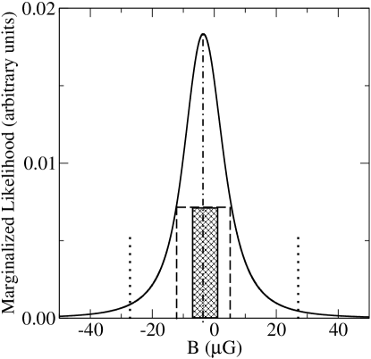
Figure 1.— Marginalized likelihood for the case of L1448CO (not normalized, heavy black line). The location of the maximum-likelihood value of $B_{0}$ is shown with the dot-dashed line. The dashed lines indicate the $1\sigma$ equilikelihood level, and the locations of the $1\sigma$ limits of $B_{0}$. The shaded box shows the allowed $1\sigma$ values for the mean envelope magnetic field for the same cloud according to CHT. Dotted lines indicate the $2\sigma$ upper limit on the absolute value of the mean envelope magnetic field.

Even if we use the (significatly underestimated, as we discussed in the previous section) overall uncertainties of CHT quoted in Table 2, and treat them as perfectly gaussian errors (which, as we have seen, is not the case), 3 of the 4 clouds do not have a statistically significant ($\geq 2\sigma$) measurement of the mean envelope magnetic field, while the 4th cloud (B1) has a marginal, $2\sigma$ measurement of the mean; even the B1 mean envelope magnetic field becomes consistent with zero if the correct uncertainties are used. As CHT point out, this is not necessarily a problem: useful limits on the ratio $R$ can be derived using upper limits for the envelope magnetic field, provided that measurements of the core magnetic field exist. However such limits, either for the envelope magnetic field or for $R$, are not calculated by the authors. Instead, nondetections are treated as detections, and the authors repeatedly refer to their “measurements” of $R$, $R^{\prime}$, and their mean. Such measurements are not, in fact, possible with the data presented in their paper. The ratio R has not been measured. However, upper limits can be placed on its value although, as we explain below, these limits are not very strong for any of the observed clouds.

We note that the proper treatment of nondetections can in principle severely constrain theories of interstellar medium evolution and core formation, if the upper limits placed are strong enough (it could, for example, be the case that the measured $3\sigma$ upper limit for $R$ is $10^{-5}$! – that would certainly be implying a very weak envelope magnetic field and a very puzzling situation for any current core formation theory). However, the magnetic field upper limits have to be correctly calculated and treated as such – and they do have to be strong enough, which is not the case at all for the data presented in CHT.

Upper limits for the (absolute value of the) mean magnitude of the line-of-sight magnetic field combining all measurements of the envelope magnetic field can be derived starting from the marginalized likelihood of the previous section. The procedure is discussed in detail in Appendix A. Utilizing the marginalized likelihood provides a very straightforward way to account for and correctly treat the asymmetric nature of the error bars in the combined observational results for the envelope magnetic field, the long non-gaussian tails, and the exact nature of the question we are trying to answer.

The $2\sigma$ upper limits for the envelope magnetic field calculated this way are given in Table 3. The values of $|B_{0}|$ and $-|B_{0}|$ which include between them a fractional area of $2\sigma$ of the marginalized likelihood for L1448CO are marked with dotted lines in Figure 1. Note that the marginalized likelihood at $-|B_{0}|$ and at $|B_{0}|$ need not have (and does not have in this case) the same value; this is frequently encountered when the robust definition of an absolute-value mean envelope $B$-field upper limit is used.

Since no measurements of the mean envelope magnetic field $|B_{\rm env}|$ have been achieved, no meaningful values of the ratio $R$ can be inferred. We can, however, use the derived upper limits to similarly place upper limits on the values of $R$. To treat the problem properly, and correctly propagate uncertainties on the measured or limited observables to the derived quantity $R$, we cannot use equation (9), since the individual uncertainties involved are large while at the same time the equation which defines $R$ (equation [7]) is nonlinear. Instead, we do a full Monte-Carlo calculation to properly derive the probability distribution for the values of R as follows. We repeat the following experiment $10^{6}$ times: we draw $I_{\rm core}$, $I_{\rm env}$, $\Delta V_{\rm core}$, $\Delta_{\rm core}$ and $B_{\rm core}$ from gaussian distributions with mean and spread equal to the measurement and uncertainty quoted in CHT (this is equivalent to assuming all errors in these quantities to be Gaussian); we draw a mean value of $B_{\rm env}$ from the marginalized likelihood of the previous section; we combine all the “mock observations” of these numbers to produce one value of $R$. We use the $10^{6}$ values of $R$ produced in this way to numerically calculate the probability distribution for $R$. We then calculate the $2\sigma$ upper limit on $|R|$ by requiring that the fractional integral of this distribution between $-R$ and $R$ be $95.4\%$. The $2\sigma$ upper limits for $|R|$ are given in Table 3. Unfortunately, none of these limits are very strong. Although this is an interesting thought experiment, much more and better quality data are required before any statement can be made with regard to comparison with any theory.

In the data presented by CHT, there is a single statistically significant, at the $3\sigma$ level, detection of the envelope magnetic field – one of the four observations of the L1544 envelope magnetic field yields a value of $22\pm 6{\,\rm\mu G}$. This measurement is consistent with the $29\,{\rm\mu G}$ $2\sigma$ upper limit that one derives if all four observations of the envelope magnetic field are combined for the particular cloud. If we use this value with its associated uncertainty to calculate an $R$ for the case of L1544, we obtain $3.62\pm 1.29$ – a marginal detection of the ratio R, with a value of a few. Again, this value is consistent with the derived overall $3\sigma$ upper limit of $5.0$ obtained for L1544 by combining all observations of the magnetic field.

Table 3 $2\sigma$ Upper Limits on the Envelope Magnetic Field (in ${\rm\mu G}$) and on $R$.

Cloud	$|B_{\rm env}|(\leq 2\sigma)$	$|R|(\leq 2\sigma)$
	$({\rm\mu G})$
L1448CO	$27$	$2.0$
B217-2	$22$	$2.9$
L1544	$29$	$5.0$
B1	$20$	$1.1$

5. Comparison with the Ambipolar-Diffusion Theory

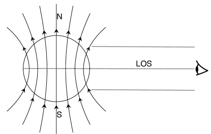
Figure 2.— Schematic diagram of a star (e.g., Sun) that has a dipolar magnetic field and is observed along lines of sight parallel to its equatorial plane. To calculate the magnetic flux threading the star, only the mean value of the magnetic field in either the northern or in the southern hemisphere is needed. If both values are averaged algebraically, the erroneous flux value of zero will be obtained.

The main conclusion of the CHT paper is that their measured values of $R$ are significantly smaller than 1, which is in contradiction with a prediction of the ambipolar-diffusion theory. We have shown above that there are, in fact, no measurements of $R$ possible with the CHT data; only weak upper limits can be placed, which have values of a few. This, however, is only part of the problem with their strongly stated conclusions.

The second error stems from the manner in which they calculate the magnetic flux of each cloud, even if their envelope magnetic fields and associated errors were to be exactly as quoted in their paper. They add algebraically the four values of the “measured” line-of-sight magnetic field strength and divide by four to obtain the mean field of the envelope. (Then they multiply this value by the area of each envelope in the plane of the sky to get the magnetic flux.) This procedure badly underestimates the envelope’s magnetic flux in at least three of the four cases, in which the envelope “measurements” show fields with opposite algebraic signs at different positions. These reversals in the direction of the magnetic field of the envelope, if real, would imply a bent magnetic flux tube threading the cloud. In such a case, only one algebraic sign of the magnetic field (the one corresponding to the greatest absolute values) should be considered in estimating the magnetic flux of the envelope. An example will clarify the point. Suppose that the dominant component of the magnetic field of a star, such as the Sun, is dipolar in nature and suppose that one wants to estimate the magnetic flux threading the star by measuring the magnetic field on the star’s surface. We assume, for simplicity, that the line-of-sight from the observer to the star lies in the star’s equatorial plane, as shown in Figure 2. If this observer did what CHT do, he would conclude that the magnetic flux of the star is exactly zero. That, of course, is far from being the case. The magnetic flux threading the star is obtained from the mean value of the magnetic field of either the sourthern or the northern hemisphere of the star (but not from the algebraic sum of the two) by multiplication with the area of the equatorial plane of the star.

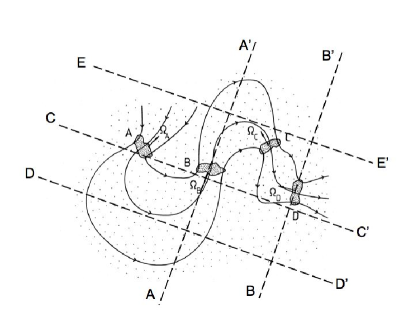
Figure 3.— Schematic diagram (from Mouschovias and Morton 1985b) of a deformed flux tube that has fragmented along its length in a molecular cloud. The deformation can be caused by the relative motion of the fragments. The fragments need not be magnetically connected for their relative motion to cause significant deformations of the field lines. The dashed lines represent different lines of sight, whose significance is explained in the text.

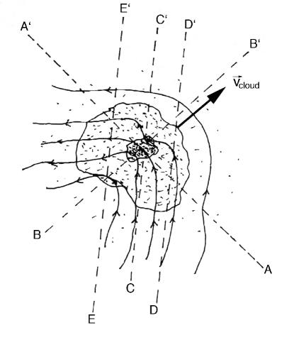
Figure 4.— Schematic diagram of the deformation of the field lines threading a cloud caused by its motion relative to the surrounding medium. The cloud is shown, for simplicity, to contain only one fragment (or core), in the neighborhood of which the hourglass shape of the field lines had been established during core formation but affected by the cloud’s motion. The dashed lines represent different lines of sight, whose significance is explained in the text.

Moreover, although CHT believe that their data reveal reversals in the direction of the magnetic field within the clouds they observe, they nevertheless compare their results with calculations that follow the formation and evolution of fragments in molecular clouds under the assumption that the parent clouds’ magnetic field lines are initially essentially straight and parallel. This idealization in the theoretical calculations renders a mathematically complicated multifluid, nonideal MHD system tractable while capturing all the essential physics of the core formation and evolution problem. However, nobody has ever suggested that in a real cloud the magnetic field lines will be essentially straight and parallel, except for the local hour-glass distortions associated with the compression of the field lines during gravitational core formation. In fact, Mouschovias & Morton (1985b, Fig. 13) had sketched what they regarded as a more realistic field geometry in a molecular cloud in which there are several (in that case four) magnetically connected fragments. That figure is reproduced here as Figure 3. This configuration can result from relative motion of the fragments (labeled A, B, C, and D in the figure) within the cloud. The motion of a cloud as a whole relative to the intercloud medium will also bend the magnetic field lines in an almost U shape, as sketched in Figure 4. One can easily visualize lines of sight in Figures 3 and 4 along which, if one were to observe $B_{\rm los}$, one would detect reversals and/or essentially vanishing $B_{\rm los}$. In other words, observations that can potentially reveal the geometry of the field lines can and should be used as input to make refinements in the theory and/or build a particular model for the cloud observed (as, for example, done in the case of B1 by Crutcher et al. 1994, and in the case of L1544 by Ciolek & Basu 2000); such observations by no means invalidate the theory, which afterall has produced dozens of predictions many of which have been confirmed by observations and none of which has been contradicted by any observation.

Figures 3 and 4 also demonstrate that the assumption by CHT, namely, that $\cos\theta$, the geometrical correction accounting for the fact that only the line-of-sight magnetic field is measurable by Zeeman observations, is the same in the core and everywhere in the envelope, is not in general valid.

The lines-of-sight labeled AA’, BB’, CC’, DD’ and EE’ in Figure 4 are chosen so as to reveal qualitatively similar behavior of the core and envelope $B_{\rm los}$ as the correspondingly labeled lines-of-sight in Figure 3. In relation to Figure 4, if an observer’s line-of-sight is the line DD’, he’ll detect essentially the full strength of the magnetic field in the nearest side of the cloud’s envelope. Along CC’, he will detect a weaker $B_{\rm los}$ in the core, although the full strength of the core’s magnetic field is clearly greater than that of the envelope, as revealed by the compressed field lines. By contrast, along the EE’ line-of-sight no envelope $B_{\rm los}$ will be detected; and along AA’, almost the full strength of the core’s magnetic field will be measured, but only a fraction of the envelope’s magnetic field strength will be detected. It is clear from this illustrutive example, which actually may not be very different from the field line geometry in a real cloud (e.g., see Brogan et al. 1999), that unless one is mindful of geometric effects, incorrect conclusions will be reached on the true magnitude of the magnetic field and, therefore, of the mass-to-flux ratio in cloud cores and envelopes. When one recalls that the relevant column density for calculating the mass-to-flux ratio is the one along a mangetic flux tube, not the one measured along an arbitrary line-of-sight, which may be at a very large angle with respect to the true magnetic field direction, one realizes that geometric effects cannot be ignored in attempts to measure or estimate the mass-to-flux ratio of a cloud or a core (e.g., see Shu et al. 1999). Simply taking the ratio of the two does not eliminate the need to account for the geometric effects.

6. SUMMARY AND CONCLUSION

We have examined critically the analysis and conclusions of recent OH Zeeman observations of four molecular cloud envelopes and cores by Crutcher et al. (2008), and we have shown that:

1. The error analysis of measurements of the envelope magnetic field is flawed, and the uncertainties on the observed mean value of the field are systematically underestimated in every cloud.

2. Although the mean value of the envelope magnetic field is not statistically significantly different from zero in any cloud, the authors treat these values as if they were detections, and they do not give appropriate upper limits.

3. If the error analysis is performed correctly, allowing possible spatial variations of the line-of-sight magnetic field (suggested by the data), and upper limits are appropriately calculated for the mean magnetic field in the envelopes, these upper limits are very weak: the mean magnetic field in the envelopes is constrained to be smaller than $20-30{\rm\,\mu G}$ at the $2\sigma$ significance level.

4. If corresponding $2\sigma$ upper limits are calculated for the value of the ratio $R$, which is given by equation (7), they are also weak: $R$ is constrained to be smaller than a few. For no cloud is the upper limit smaller than $1$. $R$ is never statistically significantly different from zero, and has not been “measured” for any cloud.

5. The magnetic fluxes of the clouds were calculated incorrectly, by averaging algebraically the (presumed) values of the line-of-sight magnetic field $B_{\rm los}$ over a cloud’s area projected on the plane of the sky, despite claimed reversals in the field direction not along one and the same line-of-sight, but from one line-of-sight to another.

6. The possible gravitational breakup (of the mass along the flux tubes threading the cores) into thermally supercritical but magnetically subcritical fragments, an effect of the ambipolar-diffusion theory studied early on (Mouschovias 1991c), was ignored by the authors. Although it is not clear whether this effect has occurred in the four clouds studied, it is nevertheless important to consider it properly before bold conclusions are drawn on the validitiy of the ambipolar- diffusion theory.

7. The ambipolar-diffusion theory can explain values of $R$ smaller than 1, especially if three-dimensional geometrical effects are properly accounted for. Although such effects are indeed missing from the published (axisymmetric) calculations against which CHT compare their observations, this is hardly new information. Focusing on effects that are known a priori to be missing from specific theoretical calculations is not a proper way to test the underlying theory or to make observational progress toward distinguishing between alternative theories. Such observations, when reliable, would provide useful input to the ambipolar-diffusion theory.

Appendix A Likelihood Approach to Error Analysis

In the classical sense, the likelihood represents the probability to have observed the data given some parent probability distribution. In the Bayesian sense, the likelihood is also proportional to the probability of the parent distribution to be described by a specific set of parameters (mean, variance) given the data. In a likelihood analysis such as the one presented here, the likelihood (properly normalized) is the probability of the set of parameters we are trying to estimate (mean, variance), as all Bayesian priors are assumed to be flat .

For simplicity, we assume that values of $B_{\rm los}$ in the envelope follow a Gaussian distribution with mean equal to $B_{0}$ and intrinsic spread $\sigma_{0}$ . If we could observe magnetic fields with zero observational error, the probability to observe a value $B$ at some specific envelope location (the likelihood $l$ of a single observation) would be $l=\exp\left[-(B-B_{0})^{2}/2\sigma_{0}^{2}\right]/\sqrt{2\pi}\sigma_{0}$. Since we have observational error, complications arise. At any specific envelope location, there is a probability $\exp\left[-(B-B_{0})^{2}/2\sigma_{0}^{2}\right]/\sqrt{2\pi}\sigma_{0}$ for the magnetic field to have a true value $B_{0}$. If the (Gaussian) observational uncertainty at this same location is $\sigma_{j}$, then the probability to observe a value $B_{j}$ of the field given that its true value is $B$ is the latter probability multiplied by a factor $\exp\left[-(B-B_{j})^{2}/2\sigma_{j}^{2}\right]/\sqrt{2\pi}\sigma_{j}$. But this is not the only way we could get an observed field value $B_{j}$. The true value of the field might be $B^{\prime}$, and we would still have a finite probability to observe $B_{j}$ (same reasoning as above, with $B$ substituted by $B^{\prime}$). To get the total probability for a single observation of $B_{j}$, we need to integrate over all possible “true” values of the magnetic field at a single location. Doing this, the likelihood for a single observation $B_{j}$ with observational uncertainty $\sigma_{j}$ becomes

$$l_{j}(B_{0},\sigma_{0})=\int_{-\infty}^{\infty}\!\!\!\!\!\!\!dB\frac{\exp\left[-(B-B_{j})^{2}/(2\sigma_{j}^{2})\right]}{\sqrt{2\pi}\sigma_{j}}\frac{\exp\left[-(B-B_{0})^{2}/(2\sigma_{0}^{2})\right]}{\sqrt{2\pi}\sigma_{0}}\,.$$ (A1)

The likelihood $\mathcal{L}$ for $N$ observations of $B_{j}$ with individual gaussian uncertainties $\sigma_{j}$ to come from a Gaussian intrinsic probability distribution with mean $B_{0}$ and spread $\sigma_{0}$ is simply the product of the individual likelihoods, $\mathcal{L}=\prod_{j=1}^{N}l_{j}$ which, after performing the integration in equation (A1) and some algebraic manipulations, yields (e.g., see Venters & Pavlidou 2007)

$$\mathcal{L}(B_{0},\sigma_{0})=\left(\prod_{j=1}^{N}\frac{1}{\sqrt{\sigma_{0}^{2}+\sigma_{j}^{2}}}\right)\exp\left[-\frac{1}{2}\sum_{j=1}^{N}\frac{(B_{j}-B_{0})^{2}}{\sigma_{0}^{2}+\sigma_{j}^{2}}\right]\,.$$ (A2)

Note that for $\sigma_{0}=0$, the value of $B_{0}$ that maximizes equation (11) is exactly the weighted average, as it should be: the weighted average formula is the maximum-likelihood estimator of the mean when the spread comes purely from observational uncertainty and the observational uncertainties are unequal.

The likelihood of equation (11) is a powerful tool that allows us to calculate the joint probability distribution of the mean $B_{0}$ and the unknown intrinsic population spread $\sigma_{0}$. However, if one wants to calculate the magnetic flux passing through a surface on which the magnetic field has a probability distribution of values, one finds that the flux integral is exactly equal to the product of the distribution mean $B_{0}$ times the surface area (in this case, modulated by $\cos\theta$ since only the line-of-sight component of the magnetic field is measured). Although we need to allow for different values of $\sigma_{0}$ to correctly estimate the uncertainty on $B_{0}$, the actual value of $\sigma_{0}$ is not of interest for the purpose of this analysis. We can therefore integrate it out of the likelihood (compute the marginalized likelihood of the mean, $\mathcal{L}_{m}=\int\mathcal{L}d\sigma_{0}$, which physically corresponds to calculating the probability distribution of the mean for any value of $\sigma_{0}$ allowed by the data). The marginalized likelihood gives the probability distribution of $B_{0}$ allowing for any possible $\sigma_{0}$ that can explain the data. The marginalized likelihood is asymmetric, and so will be the error bars. In addition, the location of the maximum-likelihood value of $B_{0}$ does not have to agree, and generally does not agree, with the estimate of the more restrictive equation (8).

To calculate uncertainties of the mean, we start from the peak of the marginalized likelihood and progressively lower the likelihood level, calculating the fractional integral under the curve and between the two values $B_{0-}$ and $B_{0+}$ left and right of the maximum-likelihood value, which are such that $\mathcal{L}_{m}(B_{0-})=\mathcal{L}_{m}(B_{0+})$. We do so until we find the $\mathcal{L}_{m}$ value for which this fractional integral is equal to $68.26\%$. The $+$ and $-$ $1\sigma$ uncertainties are then defined as $B_{0+}-B_{\rm max\mathcal{L}}$ and $B_{\rm max\mathcal{L}}-B_{0-}$, respectively.

Upper limits can also be calculated starting with the marginalied likelihood, as follows. The $2\sigma$ upper limit is that value of $|B_{0}|$ for which the area under the marginalized likelihood curve between $-|B_{0}|$ and $|B_{0}|$ is $95.4\%$. In other words, a fractional area equivalent to the gaussian $2\sigma$ is included between $-|B_{0}|$ and $|B_{0}|$. Note that, because of the different nature of the question (in this case we are interested in fixed values of $B_{0}$ rather than equal $\mathcal{L}_{m}$ likelihood levels), this is not simply the maximum-likelihood value of $B_{0}$ plus two times the error. In addition, the marginalized likelihood has much longer tails than a gaussian, and hence $1\sigma$, $2\sigma,...$ values do not scale linearly (if we desire to keep the terms representing the same fractional integrals as in the case of a gaussian).

References

- Basu & Mouschovias (1994) Basu, S., & Mouschovias, T. Ch. 1994, ApJ, 432, 720
- (2) Brogan, C. L., Troland, T. H., Roberts, D. A., & Crutcher, R. M. 1999, ApJ, 515, 304
- Ciolek & Basu (2000) Ciolek, G. E., & Basu, S. 2000, ApJ, 529, 925
- Ciolek & Mouschovias (1993) Ciolek, G. E., & Mouschovias, T. Ch. 1993, ApJ, 418, 774
- Ciolek & Mouschovias (1994) Ciolek, G. E., & Mouschovias, T. Ch. 1994, ApJ, 425, 142
- (6) Crutcher, R.M., Hakobian, N., & Troland, T.H. 2008, ApJ, submitted (arXiv:0807.2862)
- Crutcher et al. (1994) Crutcher, R. M., Mouschovias, T. Ch., Troland, T. H., & Ciolek, G. E. 1994, ApJ, 427, 839
- (8) Crutcher, R. M., Troland, T. H., Goodman, A. A., Heiles, C., Kazés, I., & Myers, P. C. 1993, ApJ, 407, 175.
- Fiebig & Guesten (1989) Fiebig, D., & Guesten, R. 1989, A&A, 214, 333
- Fiedler & Mouschovias (1992) Fiedler, R. A., & Mouschovias, T. Ch. 1992, ApJ, 391, 199
- Fiedler & Mouschovias (1993) Fiedler, R. A., & Mouschovias, T. Ch. 1993, ApJ, 415, 680
- Heiles & Crutcher (2005) Heiles, C., & Crutcher, R. M. 2005, in Cosmic Magnetic Fields, eds. R. Wielebinski & R. Beck (Berlin: Springer), 137
- (13) Lee, P. M. 2004 “Bayesian Statistics” (New York: Oxford University Press).
- (14) Lyons, L. 1992 “Statistics for Nuclear and Particle Physicists” (New York: Cambridge University Press).
- Mestel (1965) Mestel, L. 1965, QJRAS, 6, 265
- Mestel & Spitzer (1956) Mestel, L., & Spitzer, L., Jr. 1956, MNRAS, 116, 503
- Mouschovias (1977) Mouschovias, T. Ch. 1977, ApJ, 211, 147
- Mouschovias (1978) Mouschovias, T. Ch. 1978, ApJ, 224, 283
- Mouschovias (1979) Mouschovias, T. Ch. 1979a, ApJ, 228, 159
- Mouschovias (1979) Mouschovias, T. Ch. 1979b, ApJ, 228, 475
- Mouschovias (1981) Mouschovias, T. Ch. 1981, in Fundamental Problems in the Theory of Stellar Evolution, eds. D. Sugimoto, D. Q. Lamb & D. N. Schraam (Dordrecht: Reidel), 27
- Mouschovias (1987) Mouschovias, T. Ch. 1987a, in Physical Processes in Interstellar Clouds, eds. G. E. Morfill & M. Scholer (Dordrecht: Reidel), 453
- Mouschovias (1987) Mouschovias, T. Ch. 1987b, in Physical Processes in Interstellar Clouds, eds. G. E. Morfill & M. Scholer (Dordrecht: Reidel), 491
- Mouschovias (1989) Mouschovias, T. Ch. 1989, in The Physics and Chemistry of Interstellar Molecular Clouds, eds. G. Winnewisser & J. T. Armstrong (Berlin: Springer), 297
- Mouschovias (1991) Mouschovias, T. Ch. 1991a, ApJ, 373, 169
- Mouschovias (1991) Mouschovias, T. Ch. 1991b, in The Physics of Star Formation and Early Stellar Evolution, eds. C. J. Lada & N. D. Kylafis (Dordrecht: Kluwer), 61
- Mouschovias (1991) Mouschovias, T. Ch. 1991c, in The Physics of Star Formation and Early Stellar Evolution, eds. C. J. Lada & N. D. Kylafis (Dordrecht: Kluwer), 449
- Mouschovias (1996) Mouschovias, T. Ch. 1996, in Solar and Astrophysical Magnetohydrodynamic Flows, ed. K. Tsinganos (Dordrecht: Kluwer), 505
- Mouschovias & Morton (1985) Mouschovias, T. Ch., & Morton, S. A. 1985b, ApJ, 298, 205
- Mouschovias & Spitzer (1976) Mouschovias, T. Ch., & Spitzer, L., Jr. 1976, ApJ, 210, 326
- Nakano & Tademaru (1972) Nakano, T., & Tademaru, E. 1972, ApJ, 173, 87
- Nakano (1973) Nakano, T. 1973, PASJ, 25, 91
- Nakano (1976) Nakano, T. 1976, PASJ, 28, 355
- Nakano (1977) Nakano, T. 1977, PASJ, 29, 197
- Roberts (1969) Roberts, W. W. 1969, ApJ, 158, 123
- Shu, Adams & Lizano (1987) Shu, F. H., Adams, F. C., & Lizano, S. 1987, ARA&A, 25, 23
- Shu et al. (1999) Shu, F. H., Allen, A., Shang, H., Ostriker, E. C., & Li, Z.-Y. 1999, in The Origin of Stars and Planetary Systems, eds. C. J. Lada & N. D. Kylafis (Dordrecht: Kluwer), 193
- Spitzer (1968) Spitzer, L. Jr. 1968, “Diffuse Matter in Space” (New York: Wiley-Interscience)
- Tassis & Mouschovias (2007) Tassis, K., & Mouschovias, T. Ch. 2007a, ApJ, 660, 370
- Tassis & Mouschovias (2007) Tassis, K., & Mouschovias, T. Ch. 2007b, ApJ, 660, 388
- Tassis & Mouschovias (2007) Tassis, K., & Mouschovias, T. Ch. 2007c, ApJ, 660, 402
- Troland & Crutcher (2008) Troland, T. H., & Crutcher, R. M. 2008, ApJ, 680, 457
- (43) Venters, T. M. & Pavlidou, V. 2007, ApJ, 666, 128.
- Verschuur (1970) Verschuur, G. L. 1970, ApJ, 161, 867
- Verschuur (1971) Verschuur, G. L. 1971, ApJ, 165, 651
- (46) Wall, J. V & Jenkins, C. R. 2003, “Practical Statistics for Astronomers” (Cambridge, UK: Cambridge University Press).
- (47) Zuckerman, B. & Palmer, P. 1974, ARA&A, 12, 279