Control of heat transport in quantum spin systems

Abstract

We study heat transport in quantum spin systems analytically and numerically. First, we demonstrate that heat current through a two-level quantum spin system can be modulated from zero to a finite value by tuning a magnetic field. Second, we show that a spin system, consisting of two dissimilar parts - one is gapped and the other is gapless, exhibits current rectification and negative differential thermal resistance. Possible experimental realizations by using molecular junctions or magnetic materials are discussed.

When an electron moves in solids, it carries charge, spin, as well as heat. The charge degree, the basis of the modern electronics, has been fully studied over the past decades and it is still being under intensive investigation at the molecular level Datta05 ; Nitzan03 . On the other hand, the spin degree of freedom, which may be utilized to carry and process information as well, has also been explored intensively in past years, which has resulted in an emerging field “spintronics” Wolf ; RMP04 . In this context, spin (magnetization) current in insulating magnetic materials has attracted considerable attention Meier ; Sentef . However, heat current in spin systems has not been well studied as it should be.

In fact, with the rapid miniaturization and increase of operational speed of microelectronic devices, a great amount of redundant heat are produced, which will in turn affect device performance. Thus heat dissipation and heat management is becoming more and more important Schulze ; Galperin . Moreover, it was found recently that heat due to phonons can be used to carry and process information WangLi08 . Therefore, the study of heat conduction is not only of fundamental important but also helpful for the design and fabrication of heat dissipator and phononic devices. Indeed, many interesting conceptual devices such as thermal rectifier (diode) Terraneo ; Li04 ; Eckmann ; Saito06 , thermal transistor Li06 ; Ojanen , and thermal logic gate Li07 have been proposed. Experimentally, a nanoscale solid state thermal rectifier using deposited carbon nanotubes has been realized recently Chang , and a heat transistor - control heat current of electrons- controlled by a voltage gate has also been reported Saira . Furthermore, Segal and Nizan showed that thermal rectification can appear in a two-level system asymmetrically coupled to phonon baths Segal ; Segal05b , providing the possibility to control heat at a microscopic level.

In this Letter, we demonstrate that the heat part from spins can be also modulated and controlled. For example, we show that heat current in a two-level system can be modulated from zero to a finite value by tuning the magnetic field, $h$. Near $h=0$, the two levels are almost degenerate and the system can jump easily between them; thus, heat current (proportional to $h^{2}$) is small. As $h$ increases from zero to a finite value, heat current increases accordingly. We further consider a spin-$1/2$ system consists of two different segments: one is gapped and the other is gapless. We show that in such a structure thermal rectifying efficiency can be very high, up to 10 times. This system also exhibits negative differential resistance, a feature which is necessary for building up a thermal transistor.

Model For simplicity, we consider an inhomogeneous mesoscopic spin-$1/2$ chain whose Hamiltonian reads

$$H = \sum_{n=1}^{N}h_{n}\sigma_{n}^{z}-Q\sum_{n=1}^{N-1}(\sigma_{n}^{x}\sigma_{n+1}^{x}+\sigma_{n}^{z}\sigma_{n+1}^{z}),$$ (1)

where $N$ is the number of spins, the operators $\sigma_{n}^{x}$ and $\sigma_{n}^{z}$ are the Pauli matrices for the $n$th spin, $Q$ is the coupling constant between the nearest neighbor spins, and $h_{n}$ is the magnetic field strength (Zeeman splitting) at the $n$th site. Fig. 1 shows a schematic representation of this model. In the thermodynamic limit, the model is an analog of the Heisenberg spin-$1/2$ chain, wherein the heat conduction is ballistic Zotos97 ; Sologubenko00 . At the microscopic level, (1) may be viewed as a simplified version of a molecular model in low temperatures Segal05b .

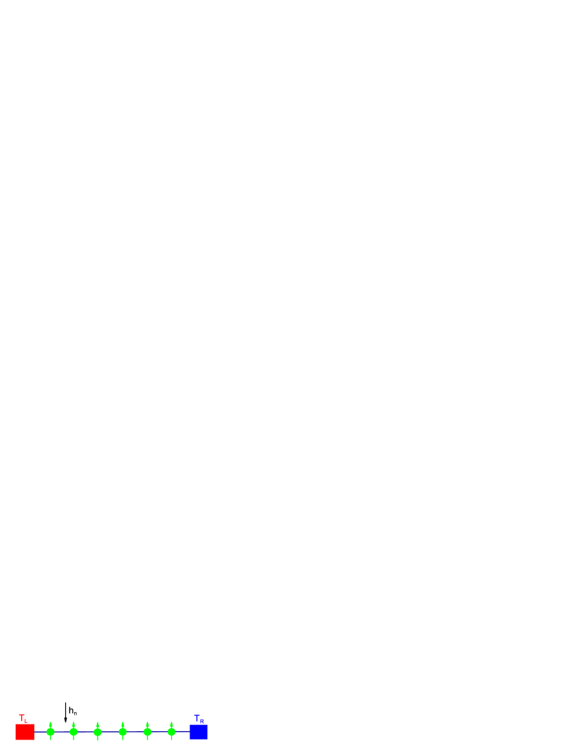
Figure 1: (color online) A schematic representation of the model with size $N=6$. The spin model is connected to two phonon baths held at different temperatures, $T_{L}$ and $T_{R}$. An inhomogeneous field is applied to introduce an asymmetric structure.

We use the quantum master equation (QME) to study heat conduction in this model. Two phononic baths of different temperatures are connected to the system at the ends. By tracing out the baths within the Born-Markov approximation, we obtain the equation of motion for the reduced density matrix of the system ($\hbar=1$) Saito ; Kubo ,

$$\frac{d\rho}{dt}=-i[H,\rho]+\mathcal{L}_{L}\rho+\mathcal{L}_{R}\rho,$$ (2)

where $\mathcal{L}_{L}\rho$ ($\mathcal{L}_{R}\rho$) is a dissipative term due to the coupling with the left (right) bath. $\mathcal{L}_{L}\rho$ is given by $\mathcal{L}_{L}\rho=\left([X_{L}\rho,\sigma^{x}_{1}]+\mathrm{H.c.}\right)$, and $\mathcal{L}_{R}\rho$ can be given in a similar way. Here the operator $X_{L}$ is defined through

$$\langle m|X_{L}|n\rangle=\lambda\varepsilon_{m,n}n_{L}(\varepsilon_{m,n})\langle m|\sigma^{x}_{1}|n\rangle,$$ (3)

where $\varepsilon_{m,n}\equiv\varepsilon_{m}-\varepsilon_{n}$, and $n_{L}(\varepsilon_{m,n})=\left(e^{\varepsilon_{m,n}/T_{L}}-1\right)^{-1}$ is the Bose distribution ($k_{B}=1$) with $T_{L}$ being the temperature of left bath. {$|n\rangle$} and {$\varepsilon_{n}$} are the eigenstates and eigenvalues of the system Hamiltonian $H$, respectively. $\lambda$ is the coupling strength with the bath. The bath spectral function we used is an Ohmic-type. The master equation (2) is solved by the fourth-order Runge-Kutta method. In numerical simulations, we take $\lambda=0.01$; the simulation time is chosen long enough such that the final density matrix $\rho$ reaches a steady state.

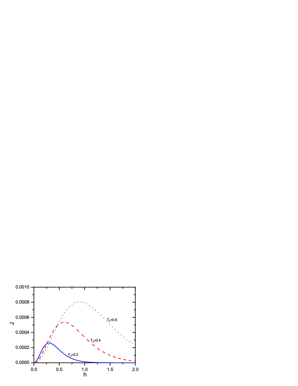
Figure 2: (color online)Modulation of Heat Current. Heat current as a function of the field. The bath temperatures are $T_{L}=T_{0}+0.05$ and $T_{R}=T_{0}-0.05$. Three cases are shown: $T_{0}=0.2$ (solid line), $T_{0}=0.4$ (dashed line), and $T_{0}=0.6$ (dotted line).

Modulation of heat current To demonstrate the modulation of heat current by an external field, we consider a simple two-level system (TLS), namely, $N=1$; thus Eq. (1) becomes $H=h\sigma^{z}$. From the QME, we obtain heat current,

$$J=\lambda(2h)^{2}\frac{n_{L}(2h)-n_{R}(2h)}{1+n_{L}(2h)+n_{R}(2h)}.$$ (4)

Fig. 2 shows heat current as a function of the field. The temperatures of the left and right baths are $T_{L}=T_{0}+0.05$ and $T_{R}=T_{0}-0.05$, respectively. $T_{0}$ is the mean temperature. In Fig. 2, we see that heat current first increases with the field and then decreases. In low fields ($h\ll T_{0}$), $n_{L,R}\sim T_{L,R}/h$, then $J\propto h^{2}$. In high fields ($h\gg T_{0}$), $n_{L,R}\sim e^{-2h/T_{L,R}}$, then $J\propto h^{3}e^{-2h/T_{0}}$, implying that heat current decays to zero when $h$ is large. Therefore, in such a model we can modulate the current from zero to a finite value by gradually switching on the external field. This result is similar to those observed in one dimensional spin-$1/2$ systems recently Sologubenko08 ; Sologubenko07 , although in our case we consider just one spin. In Fig. 2, we can also see that the current can be modulated in a much wider region in a high temperature, such as $T_{0}=0.6$.

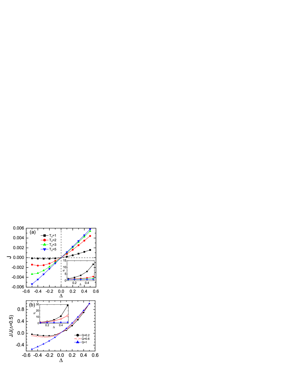
Figure 3: (color online) Rectification of Heat Current. (a) Heat current vs temperature difference. The temperatures of the baths are $T_{L}=T_{0}(1+\Delta)$ and $T_{R}=T_{0}(1-\Delta)$ where $T_{0}$ is the mean temperature, ranging from $T_{0}=1$ to $T_{0}=5$. $N=6$ and $Q=0.6$. $h_{n}=1$ if $1\leq n\leq N/2$ and $h_{n}=0$ otherwise. (b) Normalized heat current [$J/J(\Delta=0.5)$] vs $\Delta$ with different couplings. Here $T_{0}=1$. The insets show the rectification efficiency, $\eta=|J_{+}/J_{-}|$, vs the temperature difference. The lines are to guide the eye.

Rectification of Heat Current We now consider $N$ spins in an inhomogeneous magnetic field, namely, $h_{n}=1$ (as the unit of energy) if $1\leq n\leq N/2$ and $h_{n}=0$ otherwise (see Fig. 1). The temperatures of the left and right baths are $T_{L}=T_{0}(1+\Delta)$ and $T_{R}=T_{0}(1-\Delta)$, respectively, where $T_{0}$ is a mean temperature and $\Delta$ is the dimensionless temperature difference. The current operator may be defined through the equation of continuity. In Fig. 3, we show the heat current as a function of the temperature difference with the mean temperature ranging from $T_{0}=1$ to $T_{0}=5$. When the temperature is low ($T_{0}=1$), we observe that for $\Delta>0$ the heat current increases with $\Delta$, while in the region $\Delta<0$ the heat current remains very small. Thus, our model exhibits thermal rectification; namely, heat flows favorably in one direction. However, when the temperature becomes high, such as $T_{0}=5$, the magnitude of heat current changes little as the bath temperatures are exchanged. In this case the model cannot act as a good rectifier. Nevertheless, in a wide range of temperature ($T_{0}\lesssim 3$), this model shows thermal rectifying effect; the mechanism will be illustrated later. In Fig. 3(b), we show the heat current for a model with different couplings. We can see that the rectifying effect may sustain to large coupling constants. To quantify the rectification efficiency, we introduce the ratio, $\eta=|J_{+}/J_{-}|$, where $J_{+}$ is the current when $T_{L}>T_{R}$ and $J_{-}$ is the current when the temperatures are swapped, i.e., $T_{L}<T_{R}$. In a weak coupling case, e.g., $Q=0.2$, the efficiency may be more than 10 [see insets of Fig. 3(a) and (b)]; however, as the coupling $Q$ becomes stronger, the efficiency decreases.

To understand the rectifying effect qualitatively, we calculate the energy gap $E_{g}$ for a homogeneous isolated system ($h_{n}=h$) and show it in Fig. 4(a). The energy gap is obtained by calculating the energy difference between the ground state and the first excited state. In a finite field $h=1$, we observe an energy gap, $E_{g}\sim 2.8$, which is slightly dependent on the size. In the absence of the field ($h=0$), a small gap which vanishes in the thermodynamic limit is seen. Note that if the size $N$ is odd, there is no gap (degeneracy of the ground state); this is due to the particle-hole symmetry if we map the spin model to a free Fermion one by the Jordan-Wigner transformation.

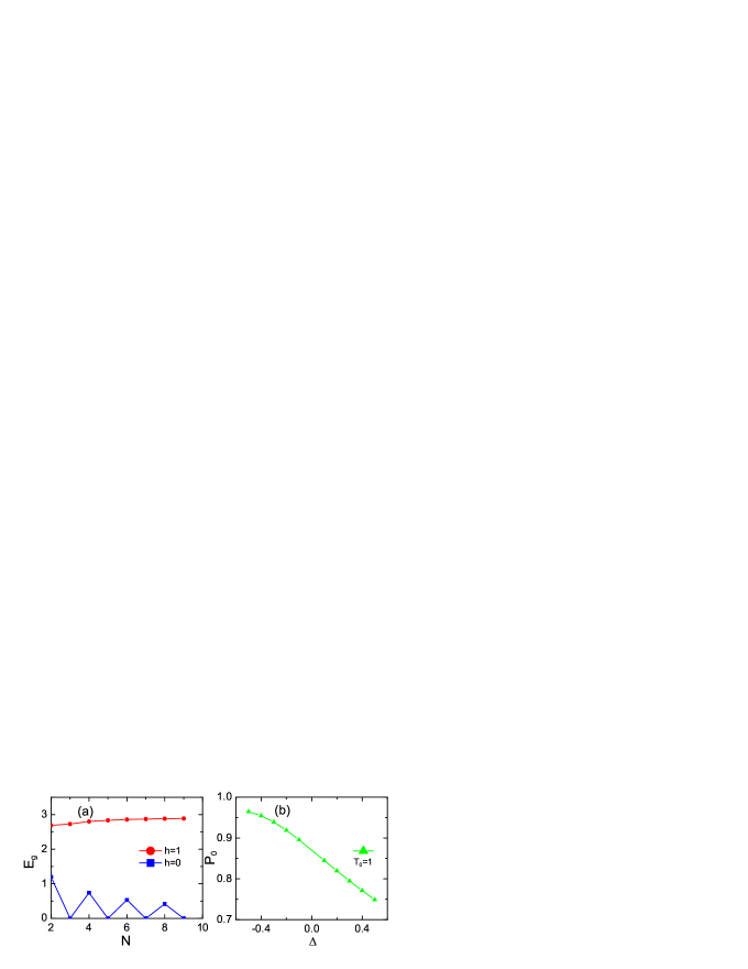
Figure 4: (color online) (a) Energy gap of an isolated homogeneous system ($h_{n}=h$) vs the system size. The gap is the energy difference between the ground state and the first excited state. $Q=0.6$. (b) The probability, $P_{0}$, to find the left part of the system in the ground state as a function of $\Delta$. $T_{0}=1$, $N=6$, $Q=0.6$, and $h_{n}=1$ if $1\leq n\leq N/2$ and zero otherwise.

At low temperatures, only a few low-lying states of each part are relevant. Therefore, if the left part (with a gap) is in contact with a cold bath and the right with a hot bath, i.e., $T_{L}=T_{c}$ and $T_{R}=T_{h}$ ($T_{c}<T_{h}$), then the left part mainly remains in the ground state. This is reflected in Fig. 4(b), which shows the probability, $P_{0}$, to find the left part in the ground state for different $\Delta$. In this case, the transition rate of the left part between different levels is low, and thus the heat current is small although the right part (no gap or a small gap) may jump easily between different levels (see also Fig. 2 for reference). Reversely, if the left part of the system is in contact with a hot bath and the right with a cold one, the transition rate of the left part between different levels is large, and then heat current becomes large. This can also explain the low rectifying efficiency when the mean temperature $T_{0}$ is increased. In this case, the transition probability of the left part between different levels may also be large; then, the magnitude of heat current changes little when the bath temperatures are exchanged, implying a low efficiency. In fact, we may observe thermal rectification provided that $T_{0}\lesssim E_{g}$.

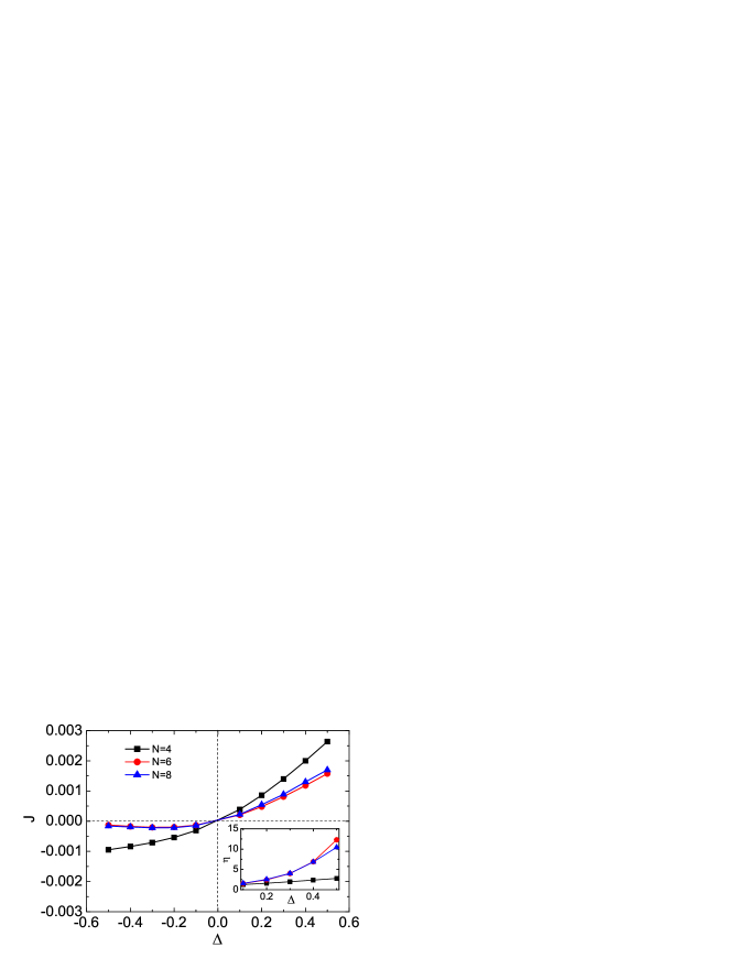
Figure 5: (color online) Rectification of Heat Current. Heat current of a system with difference sizes. The bath temperatures are $T_{L}=T_{0}(1+\Delta)$ and $T_{R}=T_{0}(1-\Delta)$. $T_{0}=1$ and $Q=0.6$. The field is $h_{n}=1$ if $n\leq N/2$ and $h_{n}=0$ otherwise. The inset shows the rectification efficiency as a function of the temperature difference.

In Fig. 5, we show the heat current for a system with different sizes. Here the coupling $Q=0.6$, and the field is $h_{n}=1$ if $n\leq N/2$ and $h_{n}=0$ otherwise. In the small size case ($N=4$), we just observe thermal rectification with a low efficiency. The reason may be that the effective coupling between the left and the right parts can be strong for a small size system. As a result, the left part may be excited by the right part even though it is connected to a cold bath. However, in a larger size system, i.e., $N=6$ or $N=8$, we may observe both thermal rectification and negative differential resistance. Note also that the efficiency changes very little when $N=6$ or $N=8$, implying that the model may act as a rectifier in an even larger size case.

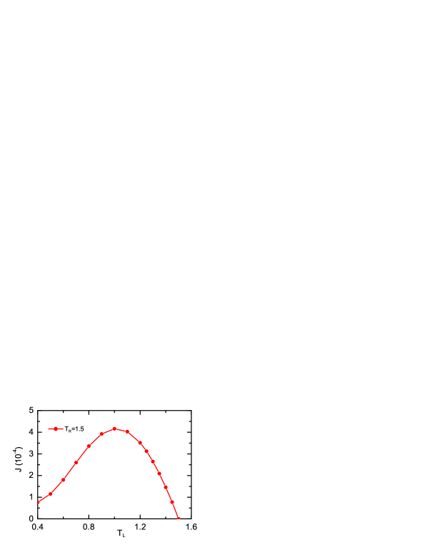
Figure 6: (color online) Negative differential thermal resistance (NDTR). Heat current vs temperature of left heat bath, $T_{L}$, with fixed $T_{R}=1.5$. The other parameters are $Q=0.6$, $N=6$, $h_{n}=1$ if $1\leq n\leq N/2$ and $h_{n}=0$ otherwise. The NTDR is clearly seen for $T_{L}<1.0$.

Negative Differential Thermal Resistance (NDTR) In fact, in Fig. 3, we can also observe NDTR in the region of $\Delta<0$, i.e., the decrease of heat current with the increase of temperature difference. A clearer representation is shown in Fig. 6, where we fix the temperature of the right bath, $T_{R}=1.5$. We see that when the temperature of the left bath $T_{L}$ is increased from $0.4$ to $1.0$, i.e., decreasing the temperature difference, thermal current increases. The reason is that: If $T_{L}$ is low, the left part is rarely excited, implying a small current; otherwise, current may become large. NDTR is an important physical property that may be used to build spin-based thermal transistors.

Summary We have studied the possibilities to control heat current in mesoscopic spin models. We have showed that heat current could be modulated from zero to a finite value in a two-level system by tuning the magnetic field. We have also studied thermal rectification and negative differential thermal resistance in an asymmetric model. The model consists of two parts: the left part is gapped, and the right part is gapless. Such a structure is of great importance for the model to exhibit rectification and NDTR. In certain cases, we have found that the rectification efficiency, $|J_{+}/J_{-}|$, can be larger than 10. Finally, we would like to discuss the possible realizations of the model in experiment. The first is to make use of the asymmetric structure in molecular bridges that can be easily introduced. For example, we may use a molecule consisting of two (weakly) coupled nonidentical spatially separated segments; each is taken to be an anharmonic system, e.g., anharmonic vibrations or molecular librations, where at low temperatures only the lowest (two) quantum states are relevant (see Fig. 1). However, in this case, there are gaps in both segments, so the rectifying effect may be not so high. The second possible way is to use magnetic materials or molecular magnets Bogani . The model may be made up of two coupled magnetic materials: one is gapped and the other is gapless. For the gapped material, one could use spin-Peierls systems or introduce a magnetic field to open a gap ($h/Q>2$) Sologubenko07 .

- (1) S. Datta, Quantum Transport: Atom to Transistor (Cambridge Univ. Press, 2005).
- (2) A. Nitzan and M. A. Ratner, Science 300, 1384 (2003).
- (3) S. A. Wolf et al., Science 294, 1488 (2001).
- (4) I. Žutić et al., Rev. Mod. Phys. 76, 323 (2004), and references therein.
- (5) F. Meier and D. Loss, Phys. Rev. Lett. 90, 167204 (2003).
- (6) M. Sentef, M. Kollar, and A. P. Kampf, Phys. Rev. B 75, 214403 (2007).
- (7) G. Schulze et al., Phys. Rev. Lett. 100, 136801 (2008).
- (8) M. Galperin, M.A. Ratner, and A. Nitzan, J. Phys.: Condens. Matter 19, 103201 (2007).
- (9) L. Wang and B. Li, Physics World 21, no 3, 27 (2008).
- (10) M. Terraneo, M. Peyrard, and G. Casati, Phys. Rev. Lett. 88, 094302 (2002).
- (11) B. Li, L. Wang, and G. Casati, Phys. Rev. Lett. 93, 184301 (2004).
- (12) J.-P. Eckmann and C. Mejia-Monasterio, Phys. Rev. Lett. 97, 094301 (2006).
- (13) K. Saito, J. Phys. Soc. Jpn. 73, 034603 (2006).
- (14) B. Li, L. Wang, and G. Casati, Appl. Phys. Lett. 88, 143501 (2006).
- (15) T. Ojanen and A.-P. Jauho, Phys. Rev. Lett. 100, 155902 (2008)
- (16) L. Wang and B. Li, Phys. Rev. Lett. 99, 177208 (2007)
- (17) C.W. Chang, D. Okawa, A. Majumdar, and A. Zettl, Science 314, 1121 (2006).
- (18) O. P. Saira et al., Phys. Rev. Lett. 99, 027203 (2007).
- (19) D. Segal and A. Nitzan, Phys. Rev. Lett. 94, 034301 (2005).
- (20) D. Segal and A. Nitzan, J. Chem. Phys. 122, 194704 (2005).
- (21) X. Zotos, F. Naef, and P. Prelovšek, Phys. Rev. B 55, 11029 (1997).
- (22) A. V. Sologubenko, E. Felder, K. Giannò, H. R. Ott, A. Vietkine, and A. Revcolevschi, Phys. Rev. B 62, R6108 (2000); A. V. Sologubenko, K. Giannò, H. R. Ott, A. Vietkine, and A. Revcolevschi, Phys. Rev. B 64, 054412 (2001).
- (23) K. Saito, Europhys. Lett. 61, 34 (2003).
- (24) R. Kubo, M. Toda, and N. Hashitsume, Statistical Physics II (Springer-Verlag, New York, 1991).
- (25) A. V. Sologubenko et al., Phys. Rev. Lett. 100, 137202 (2008).
- (26) A. V. Sologubenko, K. Berggold, T. Lorenz, A. Rosch, E. Shimshoni, M. D. Phillips, and M. M. Turnbull, Phys. Rev. Lett. 98, 107201 (2007).
- (27) L. Bogani and W. Wernsdorfer, Nature Mater. 7, 179 (2008).