Thermally activated Peierls dimerization in ferromagnetic spin chains

Abstract

We demonstrate that a Peierls dimerization can occur in ferromagnetic spin chains activated by thermal fluctuations. The dimer order parameter and entanglement measures are studied as functions of the modulation of the magnetic exchange interaction and temperature, using a spin–wave theory and the density–matrix renormalization group. We discuss the case where a periodic modulation is caused by spin–phonon coupling and the case where electronic states effectively induce such a modulation. The importance of the latter for a number of transition metal oxides is highlighted.

Structural instabilities of electronic systems can occur due to the coupling of electronic and lattice degrees of freedom (phonons). They are particularly important for quasi one–dimensional (1D) systems where the gain in electronic energy due to a lattice distortion often outweighs the cost in elastic energy. A well known example is the Peierls instability Peierls (1955) of the 1D free electron system towards a static lattice distortion determined by the Fermi momentum. For a commensurate distortion, an excitation gap is opened turning a metallic system into a band insulator. This Peierls metal–insulator transition plays an important role, for example, in organic charge–transfer solids Gruner (1955). A related instability occurs for antiferromagnetic (AFM) spin chains coupled to phonons. Here magnetic energy is gained by distorting the lattice which can lead to the so called spin–Peierls (SP) transition. Although a SP phase transition was first observed in organic materials Bray et al. (1975), it was the discovery of such a transition in CuGeO₃ by Hase et al. Hase et al. (1993) that has led to great interest in these phenomena Johnston et al. (2000).

Quite recently, another type of Peierls instability for spin chains has been found which is not driven by spin–phonon coupling but rather by a coupling of the spins with electronic degrees of freedom (orbitals). Here a ferromagnetic (FM) spin chain shows a periodic modulation (dimerization) of the magnetic exchange in a certain finite temperature region while the ground state is the uniform fully polarized FM state Sirker and Khaliullin (2003). In Ulrich et al. (2003); Horsch et al. (2003) it has been argued that this mechanism is responsible for the remarkable physical properties of YVO₃ in the finite temperature C–type AFM phase. Clearly, the lattice will react to a modulation of the magnetic exchange, however, spin–phonon coupling is not the driving force in this case and any lattice distortion is only a secondary effect.

In this Letter we want to establish general mechanisms which can drive a Peierls dimerization in FM spin chains. To highlight the differences between AFM and FM chains we will first consider a coupling to lattice degrees of freedom. The phonons are often treated adiabatically which is justified if the phonon frequency is smaller than the Peierls gap. In the adiabatic approximation the Hamiltonian can be written as $H=H_{\rm mag}+E_{\rm el}$ with

$$H_{\rm mag}=J\sum_{j=1}^{N}\left\{1+(-1)^{j}\delta\right\}\boldsymbol{S}_{j}\!\cdot\!\boldsymbol{S}_{j+1}\;,$$ (1)

and $E_{\rm el}=NK\delta^{2}/2$. Here $J$ is the exchange constant, $\boldsymbol{S}_{j}$ is a spin $S$ operator at site $j$, and $N$ is the number of sites. In the absence of a magnetic field the modulation is expected to be commensurate with wave vector $k=\pi$ and is parameterized by $\delta\in[0,1]$. The elastic energy $E_{\rm el}$ contains the elastic constant $K$. Both parameters $K,\,\delta$ can be related to the spin–phonon interaction strength. Note that writing the Hamiltonian as a sum of a magnetic and an elastic part as in Eq. (1) corresponds to the random–phase approximation (RPA) by Cross and Fisher Cross and Fisher (1978). Although the model (1) is strictly 1D, the static, mean–field (MF) treatment of the three–dimensional phonons allows for a finite temperature phase transition if $\delta(T)$ is treated as a thermodynamical degree of freedom determined by minimizing the free energy.

Let us start with the case where $\boldsymbol{S}_{j}\!\cdot\!\boldsymbol{S}_{j+1}\to S_{j}^{x}S_{j+1}^{x}+S_{j}^{y}S_{j+1}^{y}=(S^{+}_{j}S^{-}_{j+1}+S^{-}_{j}S^{+}_{j+1})/2$, i.e., we replace the SU(2)–symmetric spin exchange by an $XX$-type of interaction. In this case the sign of $J$ does not matter and the system becomes equivalent to a free spinless fermion model by Jordan–Wigner transformation. The Hamiltonian is then easily diagonalized by Fourier transformation and in the ground state for small $\delta$ one finds a gain in magnetic energy $E_{\rm mag}\sim\delta^{2}\ln\delta$. This outweighs the cost in elastic energy $E_{\rm el}\sim\delta^{2}$ and constitutes the Peierls instability for lattice fermions Pincus (1971). For the isotropic antiferromagnet ($J>0$, SU(2)–symmetric exchange), field theoretical arguments show that $E_{\rm mag}\sim-\delta^{4/3}$ Cross and Fisher (1978). Again this outweighs the cost in elastic energy leading to a SP transition and the opening of a spin gap, $\Delta\sim\delta^{2/3}$.

Contrary to the two cases discussed above there is no gain in magnetic energy in the ground state for FM coupling, $J<0$. For $\delta\in[0,1)$ the ground state is always the fully polarized FM state. We will show in the following that thermal fluctuations can, however, activate a Peierls dimerization. We will use the density–matrix renormalization group applied to transfer matrices (TMRG) to study this effect. The TMRG algorithm is based on a mapping of the 1D quantum onto a two–dimensional classical system. A transfer matrix is then defined allowing it to perform the thermodynamic limit exactly, i.e., all the numerical results presented here will be directly for the infinite system. Details of the method can be found in I. Peschel et al. (1999); Glocke et al. (2008); Sirker and Klümper (2002). In addition, we will also apply Takahashi’s modified spin–wave theory (MSWT) Takahashi (1986) to this problem.

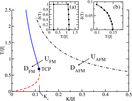
Figure 1: (color online) Phase diagrams for the dimerized AFM and FM $S=1/2$ Heisenberg chains. The dot–dashed line depicts the second order SP transition from the uniform (U) to the dimerized (D) phase for the AFM chain. For the FM chain, the D phase exists only at finite $T$ (in units of $k_{B}=1$) and only if $K<K_{c}\simeq 0.118\,|J|$ — the transition is either second or first order, as shown by solid and dashed lines, respectively, and changes its character at the tricritical point (TCP). The insets show the order parameter $\delta(T)$ for: (a) the FM chain with $K/|J|=0.1$, and (b) the AFM chain with $K/J=2$ (the lines are guides to the eye).

In Fig. 1 the phase diagrams for the $S=1/2$ isotropic AFM and FM Heisenberg models as defined in Eq. (1) are shown. The phase boundaries and order parameters are obtained using the TMRG algorithm. For the AFM we have a dimerized phase for any value of the elastic constant $K/|J|$ at low enough temperatures because the gain in magnetic energy will always win. The phase transition is second order and the evolution of the order parameter is exemplified for $K/|J|=2$ in inset (b) of Fig. 1. For the FM, on the other hand, a dimerized phase exists only at finite temperatures and only if $K/|J|<K_{c}/|J|\simeq 0.118$. Here we find a tricritical point (TCP) at $(T_{\rm TCP}/|J|,K_{\rm TCP}/|J|)\simeq(0.696,0.116)$. For $K<K_{\rm TCP}$ the transition is first (second) order if $T<T_{\rm TCP}$ ($T>T_{\rm TCP}$), respectively. Inset (a) of Fig. 1 shows that the order parameter for $K/|J|=0.1$ evolves indeed continuously at the upper phase boundary although it increases very steeply to one. Note that in the small window $K_{\rm TCP}<K<K_{c}$ both the high and the low temperature transition will be first order.

Next, we discuss the application of Takahashi’s MSWT to this problem. Usual spin–wave theory is modified by introducing a Lagrange multiplier which enforces a nonmagnetic state at finite temperature. This guarantees that the Mermin–Wagner theorem is respected. For the isotropic FM chain, results obtained by MSWT have been shown to be in excellent agreement at low temperatures with exact results obtained by the Bethe ansatz Takahashi (1987, 1986). For the dimerized chain the unit cell is doubled so that a Holstein–Primakoff transformation with different bosonic operators on the two sublattices is required. The diagonalized Hamiltonian in linear spin–wave theory is then given by $H_{\rm mag}=Ne_{0}+\sum_{k}\big{\{}\omega_{k}^{+}\beta_{k}^{\dagger}\beta_{k}+\omega_{k}^{-}\alpha_{k}^{\dagger}\alpha_{k}\big{\}}$, with $e_{0}=JS^{2}$ and the two magnon branches $\omega_{k}^{\pm}=2|J|S\left(1\pm\sqrt{\cos^{2}k+\delta^{2}\sin^{2}k}\right)$. The constraint of zero magnetization $NS=\sum_{k}\left\{n_{B}(\omega_{k}^{-})+n_{B}(\omega_{k}^{+})\right\}$ is implemented by a Lagrange multiplier $\mu$ which acts as a chemical potential with $n_{B}(\omega_{k}^{\pm})=\{\exp[(\omega_{k}^{\pm}-\mu)/T]-1\}^{-1}$ being the Bose factors. For $t/(1-\delta^{2})\ll 1$, where $t=T/(|J|S)$ is the reduced temperature, we find analytically $4S^{2}\mu/T=-t/(1-\delta^{2})+\mathcal{O}([t/(1-\delta^{2})]^{3/2})$. In the same limit the free energy per site is given by $(f-e_{0})/T=\alpha[t/(1-\delta^{2})]^{1/2}+\mathcal{O}([t/(1-\delta^{2})])$, with $\alpha=-\zeta(3/2)/(2\sqrt{\pi})$. For the FM chain we have therefore a gain in magnetic energy due to a dimerization $\sim-T^{3/2}\delta^{2}$.

To calculate spin correlation functions it is essential to take also quartic bosonic terms into account. For the bond correlations $B_{s(w)}\equiv\langle\boldsymbol{S}_{2j}\!\cdot\!\boldsymbol{S}_{2j\pm 1}\rangle$ this leads to

$$B_{s(w)}=\Big{(}\frac{1}{N}\sum_{k}\left\{n_{B}(\omega_{k}^{-})-n_{B}(\omega_{k}^{+})\right\}f^{\pm}_{k}\Big{)}^{2},$$ (2)

with $f^{\pm}_{k}=(\cos^{2}k\pm\delta\sin^{2}k)/\sqrt{\cos^{2}k+\delta^{2}\sin^{2}k}$. The plus (minus) sign in $\langle\boldsymbol{S}_{2j}\!\cdot\!\boldsymbol{S}_{2j\pm 1}\rangle$ and in $f^{\pm}_{k}$ applies for the strong (weak) bond, respectively. We define

$$\Delta^{\pm}_{SS}=\langle\boldsymbol{S}_{2j}\!\cdot\!\boldsymbol{S}_{2j+1}\rangle\pm\langle\boldsymbol{S}_{2j}\!\cdot\!\boldsymbol{S}_{2j-1}\rangle\,,$$ (3)

with $\Delta^{-}_{SS}$ acting as an order parameter for the dimerized chain. In Fig. 2 the MSWT and TMRG results for $\Delta^{-}_{SS}$ are compared for the case of $S=1$. The agreement is good for temperatures up to $T/|J|\sim 1$, in particular for small $\delta$. We also note that the MSWT gives a value in the fully dimerized case ($\delta=1$) which is in good agreement with the exact result, however, it predicts corrections for $\delta=1-\epsilon$ ($\epsilon\ll 1$) to be of order $\epsilon^{2}$, whereas the numerical results and perturbation theory show that the corrections are of order $\epsilon$. In the inset of Fig. 2 it is shown that the phase diagrams for model (1) with $S=1/2$ and $S=1$ are almost identical, if the axes are scaled appropriately.

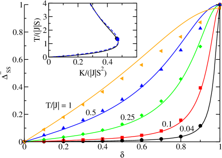
Figure 2: (color online) Order parameter $\Delta^{-}_{SS}$ (3) as a function of $\delta$ for the $S=1$ dimerized FM. The lines (symbols) denote the MSWT (TMRG) results, respectively. The inset shows the phase diagrams obtained by TMRG for the Hamiltonian (1) with $S=1/2$ (solid line) and $S=1$ (dashed line) with both axes scaled appropriately. The phase transition is first (second) order for $T<T_{\rm TCP}$ ($T>T_{\rm TCP}$). The TCP is marked by a dot (square) for $S=1/2$ ($S=1$).

In Fig. 3(a) the correlation functions on the strong and weak bond for $S=1/2$ are shown separately as a function of temperature for different $\delta$. We want to emphasize again that for $\delta\in[0,1)$ the ground state is still the usual FM state and the correlations on the weak and strong bond are thus identical, $B_{s}=B_{w}=1/4$. The difference between the correlations on the strong and on the weak bond, $\Delta^{-}_{SS}$, shown in Fig. 3(b) is therefore zero at $T=0$, goes through a maximum at some finite temperature, and goes to zero again for $T\to\infty$ where $B_{s(w)}\to 0$.

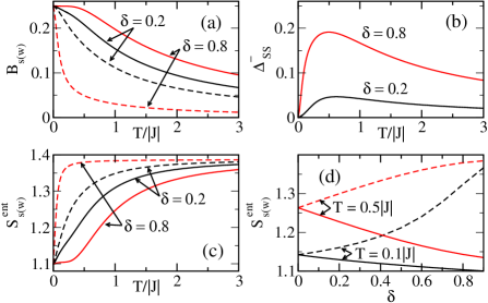
Figure 3: (color online) TMRG results for $S=1/2$: (a) $B_{s(w)}$ for the strong (solid line) and weak bond (dashed line), (b) $\Delta^{-}_{SS}$ for the same values of $\delta$ as in (a), (c) the entanglement entropy $S^{\rm\,ent}_{s(w)}$ for different $\delta$ as a function of temperature, and (d) $S^{\rm\,ent}_{s(w)}$ as a function of $\delta$ for two temperatures.

Another way of looking at the response of the FM chain to a periodic modulation is to study the entanglement of a weak or a strong bond with the rest of the system. Here we will concentrate on the case $S=1/2$. The entries of the two–qubit reduced density matrix $\tilde{\rho}$ for a bond can be related to the correlation functions on that bond Glaser et al. (2003); Pratt (2004). The concurrence for $\tilde{\rho}$ — an entanglement measure commonly used at zero temperature — can be expressed as $C_{2j,2j\pm 1}(\tilde{\rho})=2\max\{0,|\langle S^{+}_{2j}S^{-}_{2j\pm 1}\rangle|-|1/4+\langle S^{z}_{2j}S^{z}_{2j\pm 1}\rangle|\}$. It is zero for FM correlations. More interesting is the behavior of the entanglement entropy, ${\cal S}^{\rm\,ent}_{s(w)}=-\mbox{Tr}\,\tilde{\rho}\ln\tilde{\rho}$. It is again zero for the fully polarized ground state which is a pure state. At finite temperature we have for $\alpha={s(w)}$

$${\cal S}^{\rm\,ent}_{\alpha}\!=\!\Big{(}B_{\alpha}-\frac{1}{4}\Big{)}\ln\Big{(}\frac{1}{4}-B_{\alpha}\Big{)}-\!\Big{(}B_{\alpha}+\frac{3}{4}\Big{)}\ln\Big{(}\frac{1}{4}+\frac{B_{\alpha}}{3}\Big{)}\,.$$ (4)

For $T\to 0$, $B_{s(w)}\to 1/4$ and ${\cal S}^{\rm\,ent}_{s(w)}\to\ln 3$, see Fig. 3(c). ${\cal S}^{\rm\,ent}_{s(w)}$ therefore jumps signaling the phase transition at $T=0$. For $T\to\infty$, on the other hand, $B_{s(w)}\to 0$ and ${\cal S}^{\rm\,ent}_{s(w)}\to 2\ln 2$. Quite generally, the entanglement entropy for a segment with $n$ sites will go to $n{\cal S}_{T}$ for $T\to\infty$, where ${\cal S}_{T}$ is the thermal entropy per site Sorensen et al. (2007). At any fixed finite temperature the entanglement entropy ${\cal S}^{\rm\,ent}_{s(w)}$ decreases (increases) on the strong (weak) bond with increasing modulation $\delta$, see Fig. 3(d). The gain in magnetic energy at finite temperature due to a dimerization might therefore also be seen as a gain in entanglement entropy on the weak bonds.

Let us finally discuss the relevance of a thermally driven dimerization for systems with orbital degrees of freedom. This mechanism is particularly important for transition metal oxides with perovskite structure where the valence electrons are situated in the $t_{2g}$ orbitals. Because $t_{2g}$ orbitals are not bond oriented the electron–phonon coupling is weak so that we might ignore lattice degrees of freedom to first approximation. With appropriately rescaled parameters, the physics discussed below is almost independent of the spin value $S$. For definiteness, we will consider in the following the case of an effective spin $S=1$ appropriate for systems with a $3d^{2}$ valence electron configuration, as for example, YVO₃, and a twofold orbital degeneracy described by an orbital pseudospin $\tau=1/2$. A 1D Hamiltonian reflecting the spin–orbital physics for such a system is given by Khaliullin et al. (2001)

$$H_{S\tau}=J\sum_{j}\left(\boldsymbol{S}_{j}\!\cdot\!\boldsymbol{S}_{j+1}+1\right)\left(\boldsymbol{\tau}_{j}\!\cdot\!\boldsymbol{\tau}_{j+1}+\frac{1}{4}-\gamma_{H}\right),$$ (5)

where $J>0$ is the superexchange and $\gamma_{H}$ is proportional to the Hund’s coupling and promotes FM spin correlations. Using a MF decoupling, which is reasonable for FM spin correlations Oleś et al. (2006), we write $H_{S\tau}\simeq H_{S}+H_{\tau}$, where $H_{S}$ ($H_{\tau}$) is the Hamiltonian for the spin (orbital) sector, respectively. If we allow for a dimerization in both sectors then $H_{S(\tau)}$ is — up to a constant — given by Eq. (1) with $J\to J\mathcal{J}_{S(\tau)}$, $\delta\to\delta_{S(\tau)}$, and $\boldsymbol{S}$ representing the spins $S=1$ or the orbital pseudospins $\tau=1/2$, respectively. The effective superexchange constants are given by $\mathcal{J}_{S}=\Delta_{\tau\tau}^{+}/2+1/4-\gamma_{H}$ and $\mathcal{J}_{\tau}=\Delta^{+}_{SS}/2+1$, with $\Delta_{\tau\tau}^{\pm}$ defined analogously to $\Delta^{\pm}_{SS}$. Strong quantum fluctuations for pseudospin $1/2$ and $\gamma_{H}>0$ will favor AFM coupled orbitals, $\mathcal{J}_{\tau}>0$, and FM coupled spins, $\mathcal{J}_{S}<0$. The dimerizations are then given by $\delta_{S}=\Delta^{-}_{\tau\tau}/(2\mathcal{J}_{S})$ and $\delta_{\tau}=\Delta^{-}_{SS}/(2\mathcal{J}_{\tau})$. This means that the exchange constants and the dimerizations for each sector are determined by the nearest–neighbor correlations in the other sector and therefore have to be calculated self–consistently. We can simplify this procedure by noting that $\Delta^{+}_{SS(\tau\tau)}$ show only a weak dependence on dimerization and temperature for low temperatures. We therefore fix $\mathcal{J}_{S(\tau)}$ by using the values for $\Delta^{+}_{SS(\tau\tau)}$ obtained for an undimerized chain at zero temperature. This leads to $\mathcal{J}_{\tau}=2$ and $\mathcal{J}_{S}=1/2-\ln 2-\gamma_{H}$ . Now the dimerizations $\delta_{S(\tau)}$ can be easily determined self–consistently. The results for $\gamma_{H}=0.1$ — which is a realistic value for cubic vanadates — are shown in Fig. 4.

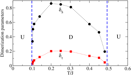
Figure 4: (color online) Phase diagram and dimerization parameters $\delta_{S},\,\delta_{\tau}$ for the spin–orbital model (5) with $\gamma_{H}=0.1$ in MF decoupling. The dashed lines denote the phase boundaries between the uniform (U) and dimerized (D) phases.

For $0.10\lesssim T/J\lesssim 0.49$ the self–consistent MF decoupling leads to nonzero values for $\delta_{S(\tau)}$. The evolution of the dimerization parameters in this temperature regime has a dome–shaped form with a maximum at $T/J\sim 0.2$. In agreement with Fig. 1, the dimerization in the FM spin chain is much larger than the dimerization in the AFM orbital chain and at $T/J=0.2$ we have $\delta_{S}\approx 0.86$ which is already close to perfect dimerization (Fig. 4). This underlines that the thermally activated dimerization in the FM chain is the driving force behind the finite temperature dimerized phase for the spin–orbital chain. The phase transitions at finite temperature between a uniform and a dimerized phase are a consequence of the MF decoupling. Such phase transitions will not occur for the strictly 1D model (5). Nevertheless, numerical calculations for this model Sirker and Khaliullin (2003) show that a dimerization is the leading instability at temperatures which support the dimerized phase in the MF decoupling solution.

Summarizing, we have shown that a dimerization can occur in FM spin chains but has to be activated by thermal fluctuations. The gain in magnetic energy at finite temperatures can be related to an increased entanglement entropy on the weak bonds. For a FM chain with spin–phonon coupling we have derived the phase diagrams as a function of temperature $T$ and the effective elastic constant $K$ for spin values $S=1/2$ and $S=1$. Thermodynamic properties of the dimerized FM chain can be calculated analytically with good accuracy for temperatures $T\lesssim|J|S$ by a MSWT. Remarkably, this approach works for all dimerizations $\delta\in[0,1]$ if quartic terms are taken into account appropriately. For a system of coupled FM spin-$1$ and AFM orbital pseudospin-$1/2$ degrees of freedom we found, using a mean–field decoupling, a finite temperature dimerized phase. This shows that a dimerization is a universal instability of FM chains at finite temperatures, and may be triggered by the coupling to purely electronic degrees of freedom. This latter mechanism seems to be relevant for many transition metal oxides with (nearly) degenerate orbital states.

The authors thank G. Khaliullin for valuable discussions. A.M. Oleś acknowledges support by the Foundation for Polish Science (FNP) and by the Polish Ministry of Science and Education Project No. N202 068 32/1481.

References

- Peierls (1955) R.E. Peierls, Quantum Theory of Solids (Oxford University Press, Oxford, 1955).
- Gruner (1955) G. Grüner, Density Waves in Solids (Addison–Wesley, Reading, MA, 2000).
- Bray et al. (1975) J.W. Bray et al., Phys. Rev. Lett. 35, 744 (1975).
- Hase et al. (1993) M. Hase, I. Terasaki, and K. Uchinokura, Phys. Rev. Lett. 70, 3651 (1993).
- Johnston et al. (2000) D.C. Johnston et al., Phys. Rev. B 61, 9558 (2000).
- Sirker and Khaliullin (2003) J. Sirker and G. Khaliullin, Phys. Rev. B 67, 100408(R) (2003).
- Ulrich et al. (2003) C. Ulrich et al., Phys. Rev. Lett. 91, 257202 (2003).
- Horsch et al. (2003) P. Horsch, G. Khaliullin, and A.M. Oleś, Phys. Rev. Lett. 91, 257203 (2003).
- Cross and Fisher (1978) M.C. Cross and D.S. Fisher, Phys. Rev. B 19, 402 (1979).
- Pincus (1971) P. Pincus, Solid State Comm. 9, 1971 (1971).
- I. Peschel et al. (1999) I. Peschel et al., eds., Density-Matrix Renormalization, Lecture Notes in Physics, vol. 528 (Springer, Berlin, 1999), and references therein.
- Glocke et al. (2008) S. Glocke, A. Klümper, and J. Sirker, in: Computational Many-Particle Physics, Lecture Notes in Physics, vol. 739 (Springer, Berlin, 2008).
- Sirker and Klümper (2002) J. Sirker and A. Klümper, Europhys. Lett. 60, 262 (2002).
- Takahashi (1986) M. Takahashi, Prog. Theor. Phys. Supp. 87, 233 (1986).
- Takahashi (1987) M. Takahashi, Phys. Rev. Lett. 58, 168 (1987).
- Glaser et al. (2003) U. Glaser, H. Büttner, and H. Fehske, Phys. Rev. A 68, 032318 (2003).
- Pratt (2004) J.S. Pratt, Phys. Rev. Lett. 93, 237205 (2004).
- Sorensen et al. (2007) E.S. Sørensen M.-S. Chang, N. Laflorencie, and I. Affleck, J. Stat. Mech.: Theor. Exp. P08003 (2007).
- Khaliullin et al. (2001) G. Khaliullin, P. Horsch, and A.M. Oleś, Phys. Rev. Lett. 86, 3879 (2001).
- Oleś et al. (2006) A.M. Oleś et al., Phys. Rev. Lett. 96, 147205 (2006).