Optimal Fourier filtering of a function that is strictly confined within a sphere

Abstract

We present an alternative method to filter a distribution, that is strictly confined within a sphere of given radius $r_{c}$, so that its Fourier transform is optimally confined within another sphere of radius $k_{c}$. In electronic structure methods, it can be used to generate optimized pseudopotentials, pseudocore charge distributions, and pseudo atomic orbital basis sets.

In some computational problems we are interested in distributions that are strictly confined within a sphere of given radius (i. e. defined to be strictly zero outside that sphere) and, simultaneously, optimally confined within another sphere in reciprocal space, so that they can be well approximated by a finite number of Fourier components or, equivalently, by a finite number of grid points in real space. Within the field of electronic structure calculations, this typically occurs in the real-space application of pseudopotentials  King-Smith et al. (1991); Briggs et al. (1996); Ono and Hirose (1999); Wang (2001); Tafipolsky and Schmid (2006). In the specific case of the SIESTA density functional method Ordejón et al. (1996); Soler et al. (2002), this problem arises in the evaluation, using a real-space grid, of matrix elements involving strictly localized basis orbitals Sankey and Niklewski (1989) and neutral-atom pseudopotentials. Those integrals produce an artificial rippling of the total energy, as a function of the atomic positions relative to the grid points (the so-called “egg box” effect), which complicates considerably the relaxation of the geometry and the evaluation of phonon frequencies by finite differences.

We have proposed recently a method to filter a distribution simultaneously in real and reciprocal space Anglada and Soler (2006). Such filter is optimal, in the sense of minimizing the norm of the function outside two spheres of radius $r_{c}$ and $k_{c}$ in real and Fourier space, respectively. It works by projecting the distribution to be filtered on a basis of functions that have the same shape in real and reciprocal space, and that are thus optimally confined in both. However, because of the uncertainty principle, such basis functions, and the resulting filtered distribution, cannot be strictly confined in any of the two spaces. Thus, if we insist in the strict confinement in real space, and therefore we truncate the filtered pseudoatomic orbitals beyond $r_{c}$, they will have a discontinuity at $r_{c}$, and therefore an infinite kinetic energy. In practice, the smallness of the discontinuity, and the use of integration grids with finite spacings, makes the problem more academic than real. But occasionally, when trying to converge the results to very high precision, it is annoying to have such a potential problem. Another, independent problem in our previous procedure is that the resulting functions, that were expanded in Legendre polynomials, do not obey exactly the correct behavior for $r\rightarrow 0$. In the present work, we propose an alternative method to filter a distribution so that it is always strictly confined in real space, while it is optimally confined in reciprocal space.

Consider an initial function with a well defined angular momentum and strictly confined within a sphere:

$$F_{0}({\bf r})=\left\{\begin{array}[]{ll}F_{0}(r)Y_{l}^{m}({\bf\hat{r}})&\mbox{if $r\leq r_{c}$}\\ 0&\mbox{otherwise,}\end{array}\right.$$ (1)

where $F_{0}(r)$ is continuous and $F_{0}(r_{c})=0$. We are using the same symbol for $F_{0}({\bf r})$ and its radial part $F_{0}(r)$, since it does not lead to any confusion. $Y_{l}^{m}({\bf\hat{r}})$ is a real spherical harmonic. To require that $F({\bf r})$ [the filtered version of $F_{0}({\bf r})$] remains strictly zero for $r>r_{c}$, and continuous at $r_{c}$ (so that its kinetic energy is finite), we will expand it in terms of spherical Bessel functions $j_{l}$ with a zero at $r_{c}$:

$$F(r)=\left\{\begin{array}[]{ll}\sum_{n=1}^{M}c_{n}N_{ln}j_{l}(k_{ln}r)&\mbox{if $r\leq r_{c}$}\\ 0&\mbox{otherwise,}\end{array}\right.$$ (2)

where $M$ is large enough to represent the function with the required accuracy, $k_{ln}r_{c}$ is the $n$th root of $j_{l}(x)$, and $N_{ln}$ are normalization constants given by

$$N_{ln}^{-2}=\int_{0}^{r_{c}}r^{2}dr~{}j_{l}^{2}(k_{ln}r)=\frac{r_{c}^{3}}{2}j_{l+1}^{2}(k_{ln}r_{c}).$$ (3)

The Fourier transform of $F({\bf r})$ is

$$G({\bf k})\equiv\frac{i^{l}}{(2\pi)^{3/2}}\int d^{3}{\bf r}~{}e^{-i{\bf k}{\bf r}}F({\bf r})=G(k)Y_{l}^{m}({\bf\hat{k}}),$$ (4)

where we have introduced the factor $i^{l}$ to make $G({\bf k})$ real, and

$$G(k)=\sum_{n=1}^{N}G_{n}j_{ln}(k),$$ (5)

where $j_{ln}(k)$ is the Fourier transform of $N_{ln}j_{l}(k_{ln}r)$:

$$j_{ln}(k) \equiv \frac{1}{(2\pi)^{3/2}}\int_{0}^{r_{c}}4\pi r^{2}dr~{}N_{ln}j_{l}(k_{ln}r)~{}j_{l}(kr)$$ (8)

$$= \left(\frac{r_{c}^{3}}{\pi}\right)^{1/2}\times\left\{\begin{array}[]{ll}j_{l+1}(k_{ln}r_{c})&\mbox{if $k=k_{ln}$}\\ -\frac{2k_{ln}r_{c}}{k^{2}r_{c}^{2}-k_{ln}^{2}r_{c}^{2}}j_{l}(kr_{c})&\mbox{otherwise.}\end{array}\right.$$

The basis functions $N_{ln}j_{l}(k_{ln}r)$ are the solutions to Schrödinger’s equation in a potential $V(r)=0$ for $r\leq r_{c}$. According to the variational principle, they are the functions that minimize the kinetic energy, among those strictly confined within a sphere of radius $r_{c}$. Some of the Fourier transforms $j_{ln}(k)$ are shown in Fig. 1. They are delta-like functions in reciprocal space, broadened because of their confinement in real space, according to the uncertainty principle.

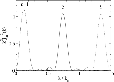
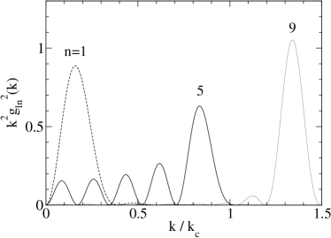
Figure 1: Upper panel: squared Fourier transform, $k^{2}j_{ln}^{2}(k)$, of some normalized spherical Bessel functions $j_{l}(k_{ln}r)$ strictly confined in $r\leq r_{c}$. Lower panel: squared Fourier transform of selected solutions, $g_{ln}(k)$, to the problem of minimizing the kinetic energy in $k>k_{c}$, Eq. (9). $l=0,k_{c}r_{c}=25$.

A conventional and straightforward method to filter $F({\bf r})$ would be to project it on the basis $j_{l}(k_{ln}r)$, with $k_{ln}<k_{c}$, i. e. by truncating the series in Eq. (2). A better procedure is to use a basis of orthonormal functions that minimize not the total kinetic energy, but specifically the kinetic energy in the region $k>k_{c}$ that we want to filter out:

$$\int_{k_{c}}^{\infty}k^{4}dk~{}g_{l}^{2}(k)=\min.$$ (9)

Expanding the solutions in the primitive basis,

$$g_{l}(k)=\sum_{n}c_{n}j_{ln}(k),$$ (10)

leads to the eigenvalue equation

$$\sum_{m}H_{nm}c_{m}=\epsilon c_{n}$$ (11)

where $\epsilon$ is a Lagrange multiplier to ensure normalization and

$$H_{nm} = \int_{k_{c}}^{\infty}k^{4}dk~{}j_{ln}(k)~{}j_{lm}(k)$$ (12)

$$= k_{ln}^{2}\delta_{nm}-\int_{0}^{k_{c}}k^{4}dk~{}j_{ln}(k)~{}j_{lm}(k).$$

The resulting eigenfunctions $g_{ln}(k)$ (that we will call “filterets”) are qualitatively very similar in real space to those in ref.[Anglada and Soler, 2006] and therefore they are not reproduced here again. Fig. 1 shows them in reciprocal space for a very small value $k_{c}r_{c}=25$, used to emphasize the effects of an extreme confinement. When $k_{ln}<<k_{c}$ or $k_{ln}>>k_{c}$, they are similar to the primitive functions $j_{ln}(k)$. For $k_{ln}\lesssim k_{c}$, however, they are considerably better confined within $k<k_{c}$.

The eigenvalues $\epsilon_{ln}$ of Eq. (11) give the integral of the kinetic energy “leaked” outside $k_{c}$:

$$\epsilon_{ln}=\int_{k_{c}}^{\infty}k^{4}dk~{}g_{ln}^{2}(k).$$ (13)

As expected, these eigenvalues are $\epsilon_{ln}\simeq 0$ for $k_{ln}<k_{c}$ and $\epsilon_{ln}\simeq k_{ln}^{2}$ for $k_{ln}>k_{c}$. They are compared in Fig. 2 with the same integral of the original functions and it can be seen that they are much smaller for $k_{ln}<k_{c}$.

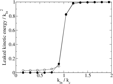
Figure 2: Leaked kinetic energy, above the cutoff $k_{c}$, of the solutions $g_{ln}(k)$ to Eq. (9) (eigenvalues $\epsilon_{ln}$, Eq. (13), filled symbols) compared to the same integral $\int_{k_{c}}^{\infty}k^{4}dk~{}j_{ln}^{2}(k)$ for the confined spherical Bessel functions (empty symbols). $l=0,k_{c}r_{c}=25$.

Since the functions $j_{ln}^{2}(k)$ minimize the total kinetic energy, the decrease of kinetic energy in $k>k_{c}$ by $g_{ln}^{2}(k)$ must be at the expense of a larger increase in $k<k_{c}$, resulting in a net increase. To control this increase, we have found convenient to give a small weight (say $w\sim 0.1$) to the kinetic energy in $k<k_{c}$. This can be done simply by multiplying the last integral in Eq. 12 by a factor $(1-w)$. A very small value $w=10^{-6}$ was used in Fig. 1, just to break the degeneracy of the functions $g_{ln}(k)$ with $k_{ln}<<k_{c}$. Larger values yield functions somewhat intermediate between both panels.

The filtered function $F({\bf r})$ is then obtained by projecting the original function $F_{0}({\bf r})$ over the subspace spanned by the “filterets” $g_{ln}^{2}(k)$ with a sufficiently low eigenvalue (say $\epsilon_{ln}/k_{ln}^{2}<0.01$). We have checked that the resulting scheme produces pseudoatomic orbitals, neutral-atom potentials Soler et al. (2002), and partial-core-correction densities Louie et al. (1982) that are free of the mentioned pathologies of the previous scheme Anglada and Soler (2006), and that reduce the “egg box” effect in SIESTA at least as well. Overall, however, the convergence tests yield rather similar results and therefore we do not repeat here the figures and tables of reference Anglada and Soler, 2006.

Finally, a practical remark on the filtering procedure is appropriate. In grid-based methods Beck (2000), in which the kinetic energy is calculated by finite differences, it is appropriate to use a filtering cutoff $k_{c}$ given by the maximum plane wave vector that can be represented in the grid without aliasing Briggs et al. (1996). In SIESTA, however, the dominant kinetic energy is calculated by well converged two-center integrals Soler et al. (2002) that do not contribute to the egg box effect. In this case, it is more convenient to fix $k_{c}$ by some independent criterion, so that the orbitals (and the kinetic energy) do not depend on the integration grid used to calculate the exchange-correlation and pseudopotential interactions. Thus, we can fix an energy threshold $\epsilon_{c}$ such that

$$\epsilon_{c}=\int_{k_{c}}^{\infty}k^{4}dk~{}\phi^{2}(k),$$ (14)

where $\phi$ are the original (unfiltered) atomic basis orbitals. This criterion will yield different (but balanced) reciprocal-space cutoffs $k_{c}$ for each orbital, in the same spirit that the “energy shift”  Soler et al. (2002) fixes their cutoffs $r_{c}$ in real space. The grid cutoff will then be fixed to $\sim 1.5-2$ times the maximum filter cutoff of all the orbitals (this factor coming from the fact that the plane wave cutoff for the density is larger than that for the wave functions).

In conclusion, we have presented a simple but powerful method to generate a basis of orthonormal functions (“filterets”), with a given angular momentum, which are strictly confined within a cutoff radius in real space and optimally confined within another cutoff in Fourier space. We have described their use to filter a function that is strictly confined within a sphere. In addition, these orthonormal functions constitute themselves a general and systematically improvable basis for converged calculations using localized basis orbitals Haynes and Payne (1997). This possibility will be explored in future works.