Indirect Dissociative Recombination of LiH${}_{2}^{+}$ + $e^{-}$

Abstract

We present the results of calculations determining the cross sections for indirect dissociative recombination of LiH${}_{2}^{+}$ + $e^{-}$. These calculations employ multichannel quantum defect theory and Fano’s rovibrational frame transformation technique to obtain the indirect DR cross section in the manner described by Ref.Hamilton and Greene (2002). We use ab initio electron-molecule scattering codes to calculate quantum defects. In contrast to H${}_{3}^{+}$, the LiH${}_{2}^{+}$ molecule exhibits considerable mixing between rotation and vibration; however, by incorporating an exact treatment of the rovibrational dynamics of the LiH${}_{2}^{+}$, we show that this mixing has only a small effect on the observed DR rate. We calculate a large DR rate for this cation, 4.0 $\times$ 10^-7 cm³ s^-1 at 1 meV incident electron energy.

I Introduction

Dissociative recombination, the process by which a cation recombines with a free electron and dissociates,

$$AB^{+}+e^{-}\longrightarrow A+B\ ,$$ (1)

has received much theoretical and experimental interest in the past two decades Florescu-Mitchell and Mitchell (2006); Larsson and Orel (2008). Innovations at both sides of the scientific process have spurred this interest. The development of storage ring experimentsLarsson (1997) has been the key innovation on the experimental side. Storage rings allow the preparation of cation species that are rovibrationally cold, such that a small number of initial rovibrational states are populated. Such devices also enable the synchronization of cation and electron beams, such that the relative kinetic energy between the two can be precisely controlled. As a result, DR rate coefficients can be determined with unprecedented resolution, and structures in the rate coefficient as a function of relative kinetic energy may be elucidated.

The current theoretical understanding of the dissociative recombination process provides two mechanisms by which it may occur. These mechanisms are labeled the “direct” and the “indirect” process. The direct process involves temporary capture of the electron into a metastable electronic state of the neutral. Such resonant electron capture was pointed out by Bates in 1950Bates (1950), and quantitatively formulated later by O’Malley in 1966O’Malley (1966); it is particularly effective in capturing low-energy (thermal) electrons when the Born-Oppenheimer potential energy curve of the metastable neutral state crosses the curve of the ground state cation species within the Franck-Condon region of the latter. It may also be the only viable mechanism of dissociative recombination at high incident electron energy.

When there is no Born-Oppenheimer curve of the neutral that crosses within the Franck-Condon region of the cation, it is the indirect mechanismGuberman (1994) that is responsible for any observed dissociative recombination. The indirect mechanism is favored by low kinetic energy of the electron-cation collision. The indirect process, like the direct process, is a resonant phenomenon; however, in this case the resonances are rovibrational Feshbach resonances, not electronic resonances as in the direct process.

Until recently, the consistent, accurate mathematical and numerical description of the indirect mechanism was elusiveOrel et al. (2000). Perhaps the most vexing problem was that of the dissociative recombination of H${}_{3}^{+}$, because the dissociative recombination of this species plays an important role in interstellar chemistry, and due to the numerous failures of theory to accurately predict the rate observed by experiment. Adding to the mystery was the considerable spread in experimental results, ranging from 2.3 $\times$ 10^-7 to less than 10^-10 cm^-3 s^-1 at 300^∘KLarsson (1997).

However, the theory outlined in Ref.Hamilton and Greene (2002), involving a frame transformation with Siegert states representing the outgoing dissociative flux, has been applied to several systems and has thus far shown consistently good results in predicting indirect DR rates. A series of theoretical worksKokoouline and Greene (2003, 2004, 2005); dos Santos et al. (2007) on the DR of H${}_{3}^{+}$ and isotopomers obtained unprecedented agreement with experiment for this difficult system, matching both the overall magnitude and most of the structure of the experimental cross sectionGlosik et al. (2001); McCall et al. (2003); Kreckel et al. (2005). Further use of the method has included a study of LiH⁺Curik and Greene (2007a, b) that reproduced the experiment of S. Krohn et al. Krohn (2001); Krohn et al. (2001) extremely well in all but the lowest part of the measured incident energy range.

In the present article, we examine the dissociative recombination of another species, namely LiH${}_{2}^{+}$. Despite any superficial similarity to H${}_{3}^{+}$, the two cations are in fact quite different, and we view these calculations as a further step toward validating and generalizing the theory. In particular, the rovibrational structure of the LiH${}_{2}^{+}$ cation is more complicated than that of H${}_{3}^{+}$; whereas Ref.Kokoouline and Greene (2003), and later, Ref.dos Santos et al. (2007) obtained excellent agreement with experiment by using a rigid rotor approximation for the vibrational states of H${}_{3}^{+}$, the LiH${}_{2}^{+}$ cation is well described as a Li⁺ cation weakly bound to an H₂ molecule, which fragments may rotate relatively independently. Thus, in the present work we incorporate an exact treatment of the rovibrational Hamiltonian and compare it to a rigid-rotor treatment. This work represents the first such exact treatment of the ionic rovibrational motion for indirect dissociative recombination in a polyatomic species.

This paper is organized as follows. We briefly introduce the electronic structure of LiH${}_{2}^{+}$ and LiH₂ in Section II. We use the the Swedish-Molecule and UK R-matrixTennyson and Morgan (1999) codes to calculate fixed-nuclei electron scattering quantum defect matrices, and we describe these calculations and present the results in Section III. A description of the calculation of the rovibrational states of the cation, including an explanation of the coordinate system we use, comprises Section IV. In Section V we describe how we account for the outgoing dissociative flux; we employ a method different from that used in previous calculations, using exterior complex scalingMcCurdy et al. (2004) instead of Siegert states to enforce outgoing wave boundary conditions on the vibrational basis. In Section VI we describe the rovibrational frame transformation and explain how the nuclear statistics are taken into account. Finally, in Section VII we present the calculated cross sections.

II Electronic structure of LiH${}_{2}^{+}$ and LiH₂

The ground electronic state of the LiH₂ molecule and the LiH${}_{2}^{+}$ cation are well described qualitatively as a Li atom or Li⁺ cation weakly bound to an H₂ molecule. Both states have an equilibrium geometry with equal Li-H bond lengths, and in such a geometry the molecule belongs to the C_2v point group. Using the labels appropriate to C_2v symmetry, the electronic configuration of the cation is 1$a_{1}^{2}$ 2$a_{1}^{2}$, for overall ²A₁ symmetry. The additional electron for LiH₂ goes into the 3$a_{1}$ orbital (approximately the Li 2$s$ orbital). When the Li-H bond lengths are unequal, the molecule belongs to the C_s point group and the cation configuration is labeled 1$a^{\prime 2}$ 2$a^{\prime 2}$.

Prior calculationsLester (1970, 1971); Kutzelnigg et al. (1973); Wagner and Wahl (1978); Wu (1979); Dixon et al. (1988); Searles and von Nagy-Felsobuki (1991); Dunne et al. (2001) have established that the equilibrium geometry of the cation has $r_{HH}$ = 1.42$a_{0}$ and $R$ = 3.62$a_{0}$, where $R$ is the distance between the Li and the H₂ center of mass. The two body asymptote Li⁺ + H₂ lies only 0.286eV higherMartinazzo et al. (2003). The three body asymptote (Li⁺ + H + H) lies much higher, 5.034eV Martinazzo et al. (2003). The LiH+ complex is weakly bound with a dissociation energy of 0.112eV and therefore this two-body breakup channel is essentially isoenergetic with the three-body channel.

Because the excitation energy of the Li⁺ cation is very high – 60.92eV – the lowest-lying electronic excitations of LiH${}_{2}^{+}$ correspond to states of the Li atom bound to a H${}_{2}^{+}$ molecule. The ionization energies of Li and H₂ are 5.39 and 15.43eV, respectively, and so we expect the first excited state to occur at roughly 10eV.

III Fixed nuclei scattering calculations on $e^{-}$ + LiH${}_{2}^{+}$

Figure 1: Quantum defect matrix elements (top two panels) and cation potential energy surfaceMartinazzo et al. (2003) (bottom panel) as a function of the Jacobi coordinate $R$, fixing $r_{HH}$ = 1.4$a_{0}$ and $\gamma$ = 90^∘. Diagonal matrix elements are labeled with a single partial wave; coupling matrix elements are labeled with the two.

Figure 2: Quantum defect matrix elements (top two panels) and cation potential energy surfaceMartinazzo et al. (2003) (bottom panel) as a function of the Jacobi coordinate $r_{HH}$, fixing $R$ = 3.62$a_{0}$ and $\gamma$ = 90^∘.

Figure 3: Quantum defect matrix elements (top two panels) and cation potential energy surfaceMartinazzo et al. (2003) (bottom panel) as a function of the Jacobi coordinate $\gamma$, fixing $R$ = 3.62$a_{0}$ and $r_{HH}$ = 1.4$a_{0}$.

The first step in the present treatment is the calculation of the fixed-nuclei quantum defect matrices, in the body frame, which describe the scattering of an electron from the LiH${}_{2}^{+}$ cation, with the positions of the nuclei frozen in space. To perform this task we employ the polyatomic UK R-matrix scattering codesTennyson and Morgan (1999) based on the Swedish-Molecule electronic structure suite.

The R-matrix calculation is defined as follows. We employed an augVTZ STO basis setEma et al. (2003) and a 20 bohr spherical R-matrix box radius. The center of mass of the LiH${}_{2}^{+}$ cation was placed at the origin. We first perform a Hartree-Fock calculation on the cation using the 1$a^{\prime 2}$ 2$a^{\prime 2}$ configuration. The target wavefunctions are defined as having the 1a^′ orbital (the Li 1s orbital) frozen in double occupation, with the remaining two electrons distributed among the space 2-6$a^{\prime}$ and 1a^′′. We keep the first nine roots of this complete active space configuration-interaction (CAS-CI) calculation to include in the scattering calculation. These correspond to the ground state, and excited states that correspond roughly to an H${}_{2}^{+}$ molecule bound to a Li atom in its $X$ ${}^{2}S$ or ${}^{2}P$ configurations, singlet or triplet coupled. Thus we have four ¹A^′ states, three ³A^′ states, and one ¹A^′′ and ³A^′′ state. At the equilibrium geometry of the cation our treatment places these states between 12.86 and 17.13eV.

To the target orbital space we add a set of uncontracted Gaussians that represent the scattering electron. This set is obtained using the UK R-matrix code GTOBASAlexandre et al. (2002), which optimizes the set to best fit a set of coulomb wavefunctions orthonormal over the R-matrix sphere. We include 15 $s$ orbitals, 13 $p$ orbitals, and 12 $d$ orbitals optimized to fit coulomb wavefunctions up to 10 hartree.

The five-electron space included in the R-matrix calculation is defined as follows. We include a close-coupling expansion corresponding to the first nine states discussed above times scattering orbitals, plus penetration terms in which all five electrons are distributed among the target orbitals, again keeping the 1$a^{\prime}$ orbital doubly occupied. The calculation is performed in overall A^′ or A^′′ symmetry.

These calculations yield the fixed-nuclei quantum defect matrices $\mu_{lm,l^{\prime}m^{\prime}}$ that are included in the later steps of the dissociative recombination calculation. The quantum defect matrix is defined in terms of the fixed-nuclei S-matrix as $\mu=-\frac{i}{2\pi}\ln(S)$. These quantum defect matrices depend weakly on the incident electron energy; we evaluate them at an incident electron energy of two meV. We construct an interpolated quantum defect matrix by splining the calculated quantum defect matrices over the Jacobi coordinate range $2.4a_{0}<R<5.6a_{0}$, $0.6a_{0}<r_{HH}<2.4a_{0}$, all $\gamma$.

Plots of the splined quantum defect surfaces are shown in Figs. 1, 2, and 3. These figures show three cuts through the quantum defect surfaces and the corresponding cuts through the cation potential energy surface; all three points contain the point ($R$=3.62$a_{0}$, $r_{HH}$=1.4$a_{0}$, $\gamma$=90^∘) in Jacobi coordinates. The cuts are in the $R$ direction (Fig. 1), the $r_{HH}$ direction (Fig. 2), and the $\gamma$ direction (Fig. 3). The convention in these figures is that all of the diagonal quantum defects are labeled and labeled with a single channel index, and some of the off-diagonal defects are labeled and labeled by the corresponding pair of indices. The molecule lies in the $yz$ plane and the vector $\vec{R}$, which connects the Li atom to the H₂ center of mass, is collinear with the $z$ axis.

For the calculation in overall A^′′ symmetry there are three electronic channels included in the R-matrix calculation, the $p_{x}$, $d_{xz}$, and $d_{xy}$. We find that the quantum defects in A^′′ symmetry are relatively small. For the calculation in overall A^′ symmetry there are six electronic channels included in the R-matrix calculation. The quantum defect matrix elements involving $p_{y}$ and $d_{x^{2}-y^{2}}$ are small relative to the other four.

IV Calculation of bound and outgoing wave rovibrational states of the cation

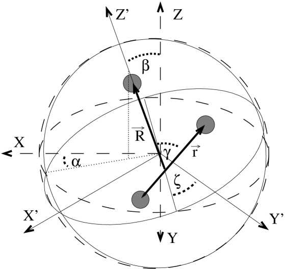
Figure 4: “R-embedding” rovibrational Jacobi coordinate system with origin at the center of mass. Primed and unprimed axes refer to BF and SF frames, respectively. The BF $x^{\prime}z^{\prime}$ and $x^{\prime}y^{\prime}$ planes are both marked with a thin line circle and the SF $xz$ and $xy$ planes are marked with dashed circles. The line of nodes is also drawn. The molecule resides in the BF $x^{\prime}z^{\prime}$ plane. The Delves hyperspherical coordinates $\theta$ and $\mathscr{R}$ used in the DR calculation are defined in terms of $R$ and $r$.

The next step in the DR treatment involves the calculation of rovibrational eigenfunctions using the ground cation potential energy surface. We employ the surface of Martinazzo et al.Martinazzo et al. (2003), which includes the proper long-range behavior of the potential.

IV.1 Coordinate system and Hamiltonian

As in previous treatmentsKokoouline and Greene (2003, 2004); Sukiasyan and Meyer (2001); dos Santos et al. (2007), we use a hyperspherical coordinate system and construct rovibrational states in an adiabatic hyperspherical basisMacek (1968). The adiabatic expansion helps to reduce the size of the calculation.

In contrast to the previous treatments we use Delves hyperspherical coordinatesDelves (1959, 1960). These coordinates are built from the Jacobi coordinate system appropriate to the system, in which $r_{HH}$ denotes the H₂ bond length, $R$ denotes the distance between the Li atom and the H₂ center of mass, and $\gamma$ denotes the angle between the two corresponding vectors. The Delves coordinates consist of the Jacobi coordinate $\gamma$, plus two additional coordinates $\mathscr{R}$ and $\theta$,

$$\begin{split}\mathscr{R}&=\sqrt{R^{2}+\frac{\mu_{r}}{\mu_{R}}r_{HH}^{2}}\\ \theta&=\tan^{-1}\left(\sqrt{\frac{\mu_{R}}{\mu_{r}}}\frac{R}{r}\right)\ .\end{split}$$ (2)

For calculations with nonzero total cation rotational angular momentum $J^{+}$, we employ the $R$-embedding coordinate systemTennyson and Sutcliffe (1982) in which the Euler angles $\alpha,\beta,\zeta$ orient the molecular $z^{\prime}$ axis, collinear with the $R$ vector, and the molecular $x^{\prime}z^{\prime}$ plane, which contains the molecule, relative to space-fixed axes. This coordinate system is depicted in Figure 4.

We employ the exact rovibrational Hamiltonian for this coordinate system, taken from its form in Jacobi coordinate system – see, for example, Refs.Petrongolo (1988); Sukiasyan and Meyer (2001).

$$\begin{split}H^{J^{+}}_{KK}=&\ \frac{1}{2\mu_{\mathscr{R}}\mathscr{R}^{2}}\Big{[}-\frac{\partial^{2}}{\partial\phi^{2}}-\frac{1}{4}+\frac{1}{\sin^{2}\theta\cos^{2}\theta}\hat{j}^{2}\\ &+\frac{1}{\sin^{2}\theta}[J^{+}(J^{+}+1)-2K^{2}+\hat{j}^{2}]\Big{]}\\ &+V(R,r,\gamma)-\frac{1}{2\mu_{\mathscr{R}}}\frac{\partial^{2}}{\partial\mathscr{R}^{2}}\\ H^{J^{+}}_{K\pm 1,K}=&\frac{1}{2\mu_{\mathscr{R}}\mathscr{R}^{2}\sin^{2}\theta}\sqrt{J^{+}(J^{+}+1)-K(K\pm 1)}\hat{j}_{\pm}\\ \hat{j}^{2}=&\ -\left(\frac{1}{{\sin}(\gamma)}\frac{\partial}{\partial\gamma}{\sin}(\gamma)\frac{\partial}{\partial\gamma}-\frac{K^{2}}{{\sin}^{2}(\gamma)}\right)\\ \hat{j}_{\pm}=&\ \mp\frac{\partial}{\partial\gamma}-K{\mathrm{cot}}(\gamma)\ .\end{split}$$ (3)

In this equation, the operators $\hat{j^{2}}$ and $\hat{j}_{\pm}$ are the total and raising/lowering operators of the diatom angular momentum. This Hamiltonian operates on the expansion coefficients $\chi_{K}$ in the following expansion of a wavefunction,

$$\Psi_{J^{+}M}=\sum_{K}\frac{\chi_{K}(\theta,\gamma,\mathscr{R})}{\mathscr{R}^{5/2}}\widetilde{D}^{J^{+}}_{MK}(\alpha,\beta,\zeta)\ ,$$ (4)

where the basis of $\widetilde{D}^{J^{+}}_{MK}(\alpha,\beta,\zeta)$ is the set of normalized Wigner rotation matrices (and BF angular momentum eigenstates)

$$\widetilde{D}^{J^{+}}_{MK}(\alpha,\beta,\zeta)=\sqrt{\frac{2J^{+}+1}{8\pi^{2}}}D^{J^{+}}_{MK}(\alpha,\beta,\zeta)\ .$$ (5)

IV.2 Coupled adiabatic hyperspherical treatment

The first step in calculating the rovibrational states is to calculate the adiabatic hyperspherical basis. Therefore, defining $H^{J^{+}}=H^{J^{+}}_{0}(\mathscr{R})-\mathscr{R}^{-5/2}\frac{1}{2\mu_{\mathscr{R}}}\frac{\partial^{2}}{\partial\mathscr{R}^{2}}\mathscr{R}^{5/2}$ where $H^{J^{+}}_{0}$ is the adiabatic Hamiltonian, we first solve for adiabatic basis functions $\chi^{J^{+}M}_{j}(\theta,\gamma,\alpha,\beta,\zeta;\mathscr{R})$ and eigenvalues $\epsilon^{J^{+}}_{j}(\mathscr{R})$ ,

$$\begin{split}H^{J^{+}}_{0}(\mathscr{R})&\chi^{J^{+}M}_{j}(\theta,\gamma,\alpha,\beta,\zeta;\mathscr{R})\\ &=\epsilon^{J^{+}}_{j}(\mathscr{R})\chi^{J^{+}M}_{j}(\theta,\gamma,\alpha,\beta,\zeta;\mathscr{R})\ ,\\ \end{split}$$ (6)

where we expand $\chi^{J^{+}M}_{j}$ as

$$\chi^{J^{+}M}_{j}(\theta,\gamma,\alpha,\beta,\zeta;\mathscr{R})=\sum_{K}\frac{\chi_{jK}^{J^{+}}(\theta,\gamma;\mathscr{R})}{\mathscr{R}^{5/2}}\widetilde{D}^{J}_{MK}(\alpha,\beta,\zeta)\ .$$ (7)

The $\alpha$-th rovibrational eigenfunction for total cation rotational angular momentum $J^{+}$ is then expanded as

$$\psi^{+}_{J^{+}M\alpha}=\sum_{ij}c^{J^{+}}_{ij\alpha}\phi_{i}(\mathscr{R})\chi^{J^{+}M}_{j}(\theta,\gamma,\alpha,\beta,\zeta;\mathscr{R}_{i})\ .$$ (8)

The coefficients $c^{J^{+}}_{ij\alpha}$ multiply basis functions $\phi_{i}(\mathscr{R})$ based on gridpoints $\mathscr{R}_{i}$. These functions comprise a Discrete Variable Representation (DVR)Dickinson and Certain (1968); Light et al. (1985); Haxton (2007), specifically, the Gauss-Lobatto finite element DVRRescigno and McCurdy (2000) with five elements 1.6 bohr long, starting at 2.0 bohr, and order 10 within each element. For the hyperangular degree of freedom $\theta$ we also use Gauss-Lobatto DVR, but with one element, and 60th order. The wavefunction is defined to be zero at $\theta$ = 0 and 90^∘. For the $\gamma$ degree of freedom we use Legendre DVR based upon associated Legendre functions $P_{lK}$. The potential is evaluated using the DVR approximation, which corresponds to a diagonal representation.

Figure 5: Rovibrational energy eigenvalues for $J^{+}$=0 and 1 (relative to three-body breakup) calculated presently with the surface of Martinazzo et al.Martinazzo et al. (2003) and the full rovibrational Hamiltonian, Eq.(3) (filled dots); those calculated for $J^{+}$=1 with a rigid rotor approximation (empty dots); and those calculated by Sanz et al.Sanz et al. (2005) with the Martinazzo surface (triangles).

To calculate the full vibrational wavefunctions including the nonadiabatic coupling, we employ the slow variable discretization of TolstikhinTolstikhin et al. (1996), and therefore solve the matrix equation for the coefficients $c^{J^{+}}_{ij\alpha}$,

$$\hat{H}^{J^{+}}\vec{c}^{J^{+}}_{\alpha}=E^{J^{+}}_{\alpha}\vec{c}^{J^{+}}_{\alpha}\ ,$$ (9)

where the matrix $\hat{H}^{J^{+}}$ is defined

$$\hat{H}^{J^{+}}_{ij,i^{\prime}j^{\prime}}=\epsilon^{J^{+}}_{j}(\mathscr{R}_{i})+\hat{O}^{J^{+}}_{ij,i^{\prime}j^{\prime}}\left(T_{\mathscr{R}}\right)_{ii^{\prime}}\ ,$$ (10)

where $T_{\mathscr{R}}$ is the Gauss-Lobatto kinetic energy matrix for the hyperradius, and where the matrix $\hat{O}^{J^{+}}$ is the overlap matrix

$$\hat{O}^{J^{+}}_{ij,i^{\prime}j^{\prime}}=\left\langle\chi^{J^{+}}_{j}(\mathscr{R}_{i})\right|\left.\chi^{J^{+}}_{j^{\prime}}(\mathscr{R}_{i^{\prime}})\right\rangle\ ,$$ (11)

brackets denoting integration over all degrees of freedom except $\mathscr{R}$.

IV.3 Rigid rotor approximation and rovibrational energies

To calculate the rigid rotor states, we calculate the vibrational states for total cation angular momentum $J^{+}=0$, obtaining their wavefunctions $\Psi^{+}_{00\alpha}$ and energies $E^{0}_{\alpha}$. We find the principal moments of inertia $A$, $B$, and $C$ for each state; the largest of these, $A$, is perpendicular to the molecular plane. We use this moment as the axis of quantization and then diagonalize the asymmetric top hamiltonian

$$\begin{split}H_{rigid}=&\frac{B+C}{4}\hat{J}^{2}+\frac{2A-B-C}{4}\hat{J}_{z}^{2}\\ &+\frac{B-C}{8}\left(\hat{J}^{+}\hat{J}^{+}+\hat{J}^{-}\hat{J}^{-}\right)\ ,\end{split}$$ (12)

in the basis $\widetilde{D}^{J^{+}}_{MK}$ for a given total cation angular momentum $J^{+}$. (In this equation, $\hat{J}^{\pm}$ are raising and lowering operators of the projection, $K$, of the total angular momentum on the body-fixed axis of quantization. They are not to be confused with the total cation angular momentum $J^{+}$, where $J^{+}(J^{+}+1)$ is the eigenvalue of the total angular momentum squared operator $\hat{J^{2}}$. $K$ is the eigenvalue of $J_{z}$. $M$ is, yet again, arbitrary.) For each value of $J^{+}$ and each $J^{+}=0$ state $\Psi^{+}_{00\alpha}$, we obtain $2J^{+}+1$ eigenvalues which are added to $E^{0}_{\alpha}$ to yield the rigid rotor energies for that vibrational state. For the purposes of the rotational frame transformation, we transform the eigenvectors of $H_{rigid}$ such that their axis of quantization, conjugate to the eigenvalue $K$, is parallel with the Jacobi vector $\vec{R}$, not perpendicular to the plane.

The $J^{+}=0$ vibrational energies (which are eqiuvalent in the rigid rotor and full rovibrational calculations) are in good agreement with the results of Sanz et al.Sanz et al. (2005). For $J^{+}>0$, The rigid rotor approximation gives significantly different low-lying eigenvalues than the full rovibrational calculation. In Figure 5 we plot the energies for rovibrational states with $J^{+}$=0 and 1. The eigenvalues of Sanz et al. for $J^{+}$=0 agree reasonably well with ours. For $J^{+}$=1 we plot eigenvalues calculated with the full Hamiltonian, Eq.(3), as well as those calculated in the rigid rotor approximation. One can clearly see that it is not accurate to treat this molecule as a rigid rotor.

Figure 6: Boltzmann weights at 300^∘ K binned by total cation angular momentum $J^{+}$.

We plot the Boltzmann weights binned by cation rovibrational angular momentum value $J^{+}$ in Figure 6. The number of rovibrational states goes as $(2J^{+}+1)^{2}$ and thus the most probable $J^{+}$ value at 300^∘ K is six.

IV.4 Nuclear statistics

The full rovibrational Hamiltonian is invariant with respect to permutations of the two hydrogen atoms. Therefore, the rovibrational eigenfunctions will have an eigenvalue of either +1 or -1 with respect to this permutation operation, which can be expressed ( $\gamma\rightarrow 90^{\circ}-\gamma$; $\zeta\rightarrow\zeta+180^{\circ}$ ). Given that the hydrogen atom is a fermion, the +1 states are paired with a singlet (para) nuclear spin wavefunction, and the -1 states are paired with a triplet (ortho) nuclear spin wavefunction. This gives the +1 and -1 states statistical weights of 1 and 3, respectively.

The full rotational/rovibrational frame transformation, described later, does not affect the nuclear statistics. However, the rovibration-only frame transformation mixes states with different permutation eigenvalues, and therefore we cannot account for the proper nuclear statistics with this transformation.

V Representation of outgoing flux

The previous implementations of the present theory have employed Siegert pseudostates Tolstikhin et al. (1998) or complex absorbing potentials (CAPs) Jackle and Meyer (1996); Leforestier and Wyatt (1983); Kosloff and Kosloff (1986) to represent the outgoing flux corresponding to dissociative recombination. In contrast, in the current implementation we employ exterior complex scaling (ECS)Aguilar and Combes (1971); Balslev and Combes (1971); Moiseyev et al. (1978); Moiseyev and Hirschfelder (1987); Lipkin et al. (1992); Moiseyev (1998); McCurdy et al. (2004) to enforce outgoing-wave boundary conditions. We have found that the use of ECS or CAP states within a MQDT frame-transformation calculation is more straightforward than the use of Siegert states, as the completeness and orthogonality relationships of the former types of eigenvectors are simpler than those of Siegert states. We will present a more thorough comparison of these different methods of enforcing outgoing-wave boundary conditions in a frame transformation calculation in a forthcoming publication.

To calculate the ECS eigenvectors, the final finite element in the $\mathscr{R}$ degree of freedom is scaled according to $\mathscr{R}\rightarrow\mathscr{R}_{0}+e^{i\theta}(\mathscr{R}-\mathscr{R}_{0})$, where $\mathscr{R}_{0}$ is the boundary between the fourth and fifth elements at $\mathscr{R}=8.4a_{0}$. We employ a scaling angle of $\frac{1}{8}\pi$. As with Siegert states, this leads to a discretized representation of the dissociative Li⁺ + H₂ vibrational continuum in which the outgoing wave states have a negative imaginary component to their energy.

Because the coordinate $\mathscr{R}$ is scaled into the complex plane, it is ideal (but often not necessaryRescigno and McCurdy (2000)) to analytically continue the potential energy surface $V(\mathscr{R},\theta,\gamma)$. We do so by ensuring that the long-range components to the Martinazzo et al. surface are evaluated for complex arguments. We evaluate their switching formula (third equation on page 11245 of their publicationMartinazzo et al. (2003)) by taking the absolute value of the argument.

VI Rovibrational frame transformation

VI.1 Introduction

The rovibrational frame transformation comprises the central part of the present calculation. Frame transformation techniques were originally developed by FanoFano (1970); Chang and Fano (1972) and have found much use in atomic and molecular theory. The central idea of a frame transformation is to take an S-matrix, which is labeled by incoming and outgoing channel indices, and transform that S-matrix to a new channel basis. In its simplest incarnation, adopted here, this transformation is exact if the fixed-nuclei quantum defects are constant with respect to energy. The transformation is accomplished via a unitary matrix that relates the first set of channels to the second. Usually, the first set of channel indices are appropriate to describe the system when the scattered electron is near the atomic or molecular target, and the second set of channel indices are appropriate when the electron has escaped far from the target. The coeffients of the original rotational frame transformation for a diatomic moleculeFano (1970) are simply Clebsch-Gordan coefficients. Other unitary transformations may be applied for different physical situations: for the calculation of Stark statesArmstrong and Greene (1994), to transform between $LS$ and $JJ$ couplingLee and Lu (1973); Robicheaux and Greene (1993), or to transform between molecular Hund’s casesJungen and Raseev (1998).

The frame transformation is applied to molecular vibration in much the same way it is applied to rotation. When the scattered electron is close to the molecule, it is moving very fast compared to the molecular framework, and therefore the scattering may be calculated by fixing the nuclei and obtaining fixed-nuclei, body-frame S-matrices $s_{lm,l^{\prime}m^{\prime}}(\vec{q})$ where $\vec{q}$ are the internal coordinates of the molecule and $lm,l^{\prime}m^{\prime}$ label the partial wave electron scattering channels in the body frame. The frame transformation provides that the full S-matrix, which has vibrational channel indices as well as electronic channel indices, is found via $S_{lm\alpha,l^{\prime}m^{\prime}\beta}=\langle\chi_{\alpha}|s_{lm,l^{\prime}m^{\prime}}|\chi_{\beta}\rangle$ where the brackets denote integration over the internal degrees of freedom $\vec{q}$.

It is important to note that this vibrational frame transformation is different from the Chase approximationChase (1956). The frame transformation is applied to the “short-range” S-matrices of Multichannel Quantum Defect Theory (MQDT)Seaton (1983); Greene et al. (1979, 1982), which have indices including not only open but also closed channels. As a result, complicated nonadiabatic effects caused by the long-range potential (here a coulomb potential) may be accounted for by the theoryRoss and Jungen (1994a, b).

The most accurate versions of the vibrational frame transformation theoryGao and Greene (1989, 1990); Gao (1992) incorporate the energy dependence of the fixed-nuclei S-matrix. We do not do so and instead evaluate the fixed-nuclei S-matrices at 2meV, implicitly making the assumption that these S-matrices are constant with respect to incident electron energy.

We note that many other treatments of dissociative recombination within MQDT have been devised. See, for example, Refs.Jungen (1984); Lee (1977). However, the current formulation is perhaps the most easily applicable to a polyatomic molecule.

VI.2 Rovibrational frame transformations for the asymmetric top

Child and JungenChild and Jungen (1990) have already derived the rotational frame transformation for the asymmetric top. We perform both a rovibration-only frame transformation and a rovibrational/rotational frame transformation that uses their result.

For the vibration-only frame transformation we calculate

$$S^{J^{+}}_{\alpha lm,\beta l^{\prime}m^{\prime}}=\left\langle\psi^{+}_{J^{+}M\alpha}\right|s_{lm,l^{\prime}m^{\prime}}\left|\psi^{+}_{J^{+}M\beta}\right\rangle\ ,$$ (13)

where value of the index $M$ is irrelevant.

The rovibrational frame transformation of Child and JungenChild and Jungen (1990) will not be repeated in full detail here. It comprises a square unitary transformation matrix for each value of $J$ (total angular momentum) and $l$ (the angular momentum of the electron). It transforms from the body-fixed representation, with quantum numbers $m$ and $K$ – denoting the projection of the electron angular momentum about the molecular axis and the projection of total angular momentum – to the space-fixed representation, with quantum numbers $J^{+}$ and $K^{+}$, denoting the total angular momentum of the cation and its projection. The body-fixed S-matrices are independent of $K$. Thus,

$$s^{J}_{lJ^{+}K^{+},l^{\prime}{J^{+}}^{\prime}{K^{+}}^{\prime}}(\mathscr{R},\theta,\gamma)=\sum_{mKm^{\prime}}U^{Jl}_{mK,J^{+}K^{+}}s_{lm,l^{\prime}m^{\prime}}(\mathscr{R},\theta,\gamma)U^{Jl^{\prime}}_{m^{\prime}K,{J^{+}}^{\prime}{K^{+}}^{\prime}}\ .$$ (14)

The full rovibrationally and rotationally transformed S-matrix is then

$$S^{J}_{J^{+}\alpha l,{J^{+}}^{\prime}\beta l^{\prime}}=\left\langle\psi^{+}_{J^{+}M\alpha}\right|\Bigg{[}\sum_{K^{+}{K^{+}}^{\prime}}\left|K^{+}\right\rangle s^{J}_{lJ^{+}K^{+},l^{\prime}{J^{+}}^{\prime}{K^{+}}^{\prime}}\left\langle{K^{+}}^{\prime}\right|\Bigg{]}\left|\psi^{+}_{J^{+}M\beta}(\mathscr{R}_{i})\right\rangle\ .$$ (15)

The index $M$ is again irrelevant.

VI.3 Channel closing and dissociative recombination cross section

The final step in the present theory is the construction of the physical, open-channel S-matrix in terms of the closed-channel S-matrices calculated from the frame transformation. Whereas the latter are assumed to be energy-independent, a strong energy dependence is introduced to the former by the formulaKokoouline and Greene (2003)

$$\begin{split}\mathscr{S}(E)&=S_{oo}-S_{oc}\left(S_{cc}-e^{-2i\beta(E)}\right)^{-1}S_{co}\\ \beta(E)&=\frac{\pi\delta_{ij}}{\sqrt{2(E_{i}-E)}}\ ,\\ \end{split}$$ (16)

where the subscript $c$ and $o$ denote the closed and open channel subblocks of the MQDT S-matrix $S^{J^{+}}$ or $S^{J}$, and we introduce the notation $\mathscr{S}$ for the physical S-matrix.

Because the higher-energy rovibrational states lie above the dissociation energy to Li⁺ + H₂, they have outgoing-wave components and negative imaginary components to their energy. As a result, the physical S-matrix is subunitary and we assign the missing part to dissociative recombination. Thus, for the vibration-only transform, we sum over the contributions of each partial wave in the electronic channel,

$$\sigma^{J^{+}}_{\alpha}(E)=\frac{\pi}{2E}\sum_{lm}\left(1-\sum_{l^{\prime}m^{\prime}\beta}\left|\mathscr{S}^{J+}_{lm\alpha,l^{\prime}m^{\prime}\beta}\right|^{2}\right)\ ,$$ (17)

and for the full rotational plus vibrational frame transformation,

$$\sigma^{J}_{J^{+}\alpha}(E)=\frac{\pi}{2E}\sum_{l}\left(1-\sum_{{J^{+}}^{\prime}l^{\prime}\beta}\left|\mathscr{S}^{J}_{J^{+}l\alpha,{J^{+}}^{\prime}l^{\prime}\beta}\right|^{2}\right)\ .$$ (18)

where $\alpha$ and $J^{+}$ denote the initial rovibrational state.

We Boltzmann-average these results, assuming a cation temperature of 300^∘ K. Thus Kokoouline and Greene (2003),

$$\sigma_{vib}(E)=\frac{1}{\Xi}\sum_{J^{+}\alpha}\ (2J^{+}+1)\ \sigma^{J^{+}}_{\alpha}(E)e^{\frac{-E_{J^{+}\alpha}}{kT}}$$ (19)

$$\sigma_{rot}(E)=\frac{1}{\Xi}\sum_{JJ^{+}\alpha}\ \frac{2J+1}{2J^{+}+1}\ \sigma^{J}_{J^{+}\alpha}(E)e^{\frac{-E_{J^{+}\alpha}}{kT}}$$ (20)

$$\Xi=\sum_{J^{+}\alpha}\ (2J^{+}+1)\ e^{\frac{-E_{J^{+}\alpha}}{kT}}$$ (21)

with T=300^∘ K.

Finally, we convolute the results with respect to the uncertainty in the incident electron kinetic energy. For the present results we use a standard deviation of $\sqrt{2}$ meV in both the parallel and transverse directions, and perform the averaging as described in Ref.Curik and Greene (2007b).

VII Results: dissociative recombination cross sections

Figure 7: Raw output of frame transformation calculation. Plotted is the dissociative recombination probability for the $J^{+}$=2 vibrational ground state, $s$-wave channel. Top, result with full rovibrational Hamiltonian; bottom, result with rigid rotor states.

Figure 8: Calculated dissociative recombination rate at 300^∘K, assuming experimental resolution of $\sqrt{2}$ meV in the parallel and transverse directions. The rotational plus rovibrational curve is our final result, and the other two curves are from the rovibrational transform only, using rigid rotor or full rovibrational states.

We seek to determine how relevant the inclusion of the exact cation rovibrational dynamics is to the experimentally observed DR rate. The raw DR cross sections that we calculate show considerable structure that depends upon whether an exact or rigid-rotor treatment of the rovibrational dynamics is used. However, experiments operate with a thermal sample of cation targets, including many rovibrational states, and use a beam of electrons with a small spread in energies. Storage-ring experiments are performed with cool cation targets, with rovibrational temperatures typically on the order of 300^∘ K. In order to compare with results obtained under these conditions, we Boltzmann-average over approximately 300 initial rovibrational states of the LiH${}_{2}^{+}$ cation, and account for the uncertainty in the incident electron energy, taken here to be 2meV ($\sqrt{2}$meV in the parallel and transverse directions). In doing so, much of the structure in the DR cross section is lost, and we find that the rigid rotor treatment is probably sufficient for calculating rates to be compared with experiment.

An example of the structure in the unconvolved cross sections is shown in Fig. 7. There we show raw results of the rovibration-only frame transformation calculation for $J^{+}$=2, both using the full rovibrational Hamiltonian to calculate the rovibrational states, and using a rigid rotor approximation for the rovibrational states. The results are markedly different, showing that the strong mixing of rotation and vibration in LiH${}_{2}^{+}$, even at low $J$, affects the structure in the cross sections for individual entrance and exit channels.

The first excited rovibrational state lies at 7.3meV. The sixth and ninth excited state, corresponding to excitation in the dissociative $R$ direction and excitation in the $\gamma$ direction – rotation of the H₂ – lie at 53meV and 77meV, respectively. As is clear from Figure 7, there is a prominent series of narrow rydberg resonances converging to the 53meV threshold, which serve to enhance the DR rate. It is therefore clear that excitation in the dissociative direction plays the largest role in the indirect DR process for this molecule, as opposed to rotational excitation or excitation in the H₂ stretch coordinate.

For the purpose of calculating rates to be compared with experiment, we find that the rigid rotor treatment is probably sufficient, though it apparently overestimates the cross section slightly. Not including the rotational frame transformation of Child and Jungen, we have compared the rovibration-only frame transformation using the full rovibrational states to that using the rigid rotor states. We find that the rigid-rotor treatment yields a DR rate consistently about 20% higher than the full rovibrational treatment. The full calculation, employing the rotation/rovibrational frame transformation and the full rovibrational states, was not completed, due to numerical difficulty. Instead, we perform the rotational transformation of Child and Jungen with the rovibrationally transformed S-matrix calculated from rigid-rotor states. On the basis of the comparison between the calculations not including the rotational transformation of Child and Jungen, we estimate that this treatment probably overestimates the cross section by about 20%.

Our convolved results are shown in Figure 8. We show the DR rate calculated at 300^∘K and including states up to $J^{+}$=9 (for the rovibration-only transformations) or $J$=11 (for the rotational and rovibrational transformation). We show three results: from using the full rovibrational Hamiltonian, with no rotational transform; from using a rigid rotor approximation, with no rotational transform; and from using a rigid rotor approximation, with the rotational transformation of Child and Jungen. The former two calculations demonstrate the effect of including the full rovibrational dynamics, and as mentioned immediately above, the rigid rotor result exceeds the full rovibrational result by approximately 20 percent, which factor is fairly independent of the incident electron energy. The latter calculation should be considered our final result, with the caveat that it probably overestimates the rate by about 20%. Nuclear statistics are included for the full rotational/rovibrational transformation, but not for the rovibration-only transformation, because the rovibration-only frame transformation destroys the permuation symmetry of the overall wavefunction. The rates are comperable but a bit higher than the corresponding rates for H${}_{3}^{+}$, by a factor of two or three. The effect of including the rotational part of the transformation is to further lower the results by about 10% in the low-energy region, and 50% in the high-energy region.

VIII Conclusion

We have applied the method of Ref. Hamilton and Greene (2002) to the calculation of the indirect DR rate of LiH${}_{2}^{+}$ + $e^{-}$. A central aim of our treatment was to analyze the effect of including the full rovibrational dynamics of the cation. We have found that although the full rovibrational treatment produces channel energies and unconvolved cross sections considerably different from a rigid rotor treatment, a rigid rotor treatment is amenable to the calculation of convolved cross sections to be compared with experiment, although it probably overestimates the DR rate for a floppy molecule such as LiH${}_{2}^{+}$ by a small and energy-independent amount.

The main approximation in the present treatment is the use of energy-independent quantum defects. For the calculation of indirect DR rates for the present system, this approximation is expected to be very good, because the amount of energy transferred from electronic to nuclear motion is rather small due to the small dissociation energy of LiH${}_{2}^{+}$. Methods to accurately treat the energy dependence of the fixed-nuclei s-matrix within a frame transformation exist Gao and Greene (1989, 1990); Gao (1992) and may be applied to this system in future work.

The calculations presented here demonstrate that the indirect mechanism provides a powerful mechanism for dissociative recombination of LiH${}_{2}^{+}$ + e^-. Future work will seek to analyze the branching ratios for two- and three-body dissociation and to further study the nature of the indirect DR mechanism.