Semiclassical Theory of Time-Reversal Focusing

Abstract

Time reversal mirrors have been successfully implemented for various kinds of waves propagating in complex media. In particular, acoustic waves in chaotic cavities exhibit a refocalization that is extremely robust against external perturbations or the partial use of the available information. We develop a semiclassical approach in order to quantitatively describe the refocusing signal resulting from an initially localized wave-packet. The time-dependent reconstructed signal grows linearly with the temporal window of injection, in agreement with the acoustic experiments, and reaches the same spatial extension of the original wave-packet. We explain the crucial role played by the chaotic dynamics for the reconstruction of the signal and its stability against external perturbations.

The concept of time reversal has captured the imagination of physicists for more than a century, leading to a vast theoretical oeuvre, sempiternal discussions, and a few concrete experimental realizations. Among them, the works on spin echoes have been of paramount importance concerning the limits in the reconstruction of an initially prepared quantum state cit-Hahn ; cit-Zhang . The time reversal of acoustic waves in a non-homogeneous medium was another experimental deed showing that an initially localized pulse can be accurately reconstructed by an array of receiver-emitter transducers that re-inject the recorded signal cit-Derode . Re-focusing of elastic, as well as electromagnetic, waves has been later achieved cit-Draeger ; cit-Catheline ; cit-Lerosey . These experiments provoke a natural surprise while yielding reconstructions, that albeit not perfect, are highly faithful. The relevant questions that arise when trying to understand these physical realizations of time reversal are related with how good a reconstruction can be achieved and which are the limits set by interactions with the environment and unavoidable errors in the reversal protocol.

In the spin echo experiments the complexity of the physical system has emerged as a critical component, and the term of Loschmidt echo (LE) has been coined to describe setups where many-body physics or chaotic dynamics are relevant cit-Levstein . In particular, the decay of the LE with the reversal time has been shown to depend on the underlying classical dynamics cit-Peres ; cit-Jalabert ; cit-Gorin : classically chaotic systems exhibit a decay rate which, for large perturbations, is bounded by the Lyapunov exponent characterizing the dynamics.

In the time-reversal mirror (TRM) procedure the play back signal builds up in the region of the original excitation, in the form of a reversed wave amplitude cit-Derode . Thus, the TRM can be viewed as the wave version of the LE. A salient feature of the TRM experiments is that, even though reversal is not perfect cit-Pastawski , the refocusing improves when the wave-propagation occurs in a disordered medium or in a chaotic cavity, as compared with the homogeneous or integrable case. Remarkably, a single transducer is enough in the case of a chaotic cavity cit-Draeger . The asymptotic analysis of the Wigner transform of wave fields in the high-frequency limit has been used to understand how multiple scattering enhances the spatial resolution of the refocused signal cit-Bal . Diagrammatic perturbation theory has been able to account for the symmetry-induced interference enhancements in the refocalization observed in disordered media cit-deRosny . The refocusing experiments in chaotic cavities have been confronted with numerical simulations cit-Draeger , as well as ergodicity and control theory cit-Bardos . The contrasting stability properties of TRM with wave and particle propagation through a multiple scattering medium has been discussed in Ref. cit-snie .

In this work we develop a semiclassical approach for TRM in chaotic cavities and quantify the quality of the reconstructed signal in terms of temporal and spatial dispersions, as well as possible environmental influences. We demonstrate the crucial role played by the underlying classical dynamics and validate our analytical results by confronting them to numerical simulations.

A high-frequency signal emitted at $t=0$ at a position $\mathbf{r}_{0}$ inside the cavity can be interpreted within the ray picture as an initial wave-packet centered at $\mathbf{r}_{0}$ that evolves and is recorded by a receiver (or an array of receivers) at position(s) $\mathbf{r}_{i}$ ($i=1,2,\ldots,N$) for times in the interval $(t_{1},t_{2})$. After a waiting time $t_{W}>t_{2}$ the re-emission of the time-reversed signal is performed in the interval $(t_{2}^{\prime}=2t_{W}-t_{2},t_{1}^{\prime}=2t_{W}-t_{1})$. The refocusing is expected at $2t_{W}$, that is redefined as the time origin for refocusing cit-Draeger (see Fig. 1(a)). The signal that can be detected in a point $\mathbf{r}$ at a time $t$ is cit-Tanner

$$\mathcal{F}_{\mathbf{p}_{0}}(\mathbf{r},t)= \sum_{i}\int_{t_{1}}^{t_{2}}\mathrm{d}\tau\ G(\mathbf{r,r}_{i},t+\tau)$$

$$\times\int\mathrm{d}\mathbf{r}^{\prime}\ G^{\ast}(\mathbf{r}_{i},\mathbf{r}^{\prime},\tau)\psi_{\mathbf{p}_{0}}^{\ast}(\mathbf{r}^{\prime})\ .$$ (1)

The propagator $G(\mathbf{r},\mathbf{r}_{i},t+\tau)$ corresponds to the re-emitted signal, which is obtained by time-reversing the evolution of the initial state with the propagator $G(\mathbf{r}_{i},\mathbf{r}^{\prime},\tau)$. We do not write the initial temporal arguments of the propagators, as they are taken to be $0$. We work in two dimensions and choose as an initial state a Gaussian wave-packet

$$\psi_{\mathbf{p}_{0}}(\mathbf{r}^{\prime})=\frac{1}{\sqrt{\pi}\sigma}\exp\left[\tfrac{\mathrm{i}}{\hbar}\mathbf{p}_{0}\cdot({\mathbf{r}}^{\prime}-\mathbf{r}_{0})-\tfrac{(\mathbf{r}^{\prime}-\mathbf{r}_{0})^{2}}{2\sigma^{2}}\right]\ ,$$ (2)

centered around $\mathbf{r}_{0}$ and with dispersion $\sigma$. The initial momentum $\mathbf{p}_{0}$ sets the energy and direction of the original signal. The choice of a quantum formalism to represent the ray picture is motivated by convenience, as we are leaving aside the delicate issue concerning a quantal recording-emission process. The quantum formalism is suited to work with the semiclassical propagator cit-Brack

$$G(\mathbf{r}^{\prime\prime},\mathbf{r}^{\prime},\tau)=\frac{1}{2\pi\mathrm{i}\hbar}\sum_{s(\mathbf{r}^{\prime},\mathbf{r}^{\prime\prime},\tau)}\sqrt{C_{s}}\ e^{\mathrm{i}S_{s}/\hbar-\mathrm{i}\frac{\pi}{2}\mu_{s}},$$ (3)

given as a sum over classical trajectories $s$ traveling in a time $\tau$ between the two extreme points. We note $S_{s}=S_{s}(\mathbf{r}^{\prime\prime},\mathbf{r}^{\prime},\tau)$ the action integral along the path, $\mu_{s}$ the Maslov index, and $C_{s}=|\mathrm{det}(-\partial S_{s}/\partial\mathbf{r}^{\prime}\partial\mathbf{r}^{\prime\prime})|$.

Performing the $\mathbf{r}^{\prime}$-integral of Eq. (1) by stationary-phase (see Ref. cit-Goussev for the precise conditions of validity of such an approximation in a chaotic cavity) we can write, for a single transducer,

$$\mathcal{F}_{\mathbf{p}_{0}}(\mathbf{r},t)= \frac{\sigma}{2\pi^{3/2}\hbar^{2}}\int_{t_{1}}^{t_{2}}\mathrm{d}\tau\sum_{s^{\prime}(\mathbf{r}_{i},\mathbf{r,}\tau+t)}\sum_{s(\mathbf{r}_{0},\mathbf{r}_{i},\tau)}\sqrt{C_{s^{\prime}}C_{s}}$$

$$\times\exp\left[\tfrac{\mathrm{i}}{\hbar}(S_{s^{\prime}}-S_{s})-\mathrm{i}\tfrac{\pi}{2}(\mu_{s^{\prime}}-\mu_{s})\right.$$

$$\left.-\tfrac{\sigma^{2}}{2\hbar^{2}}(\mathbf{p}_{s}-\mathbf{p}_{0})^{2}\right]\ ,$$ (4)

where $\mathbf{p}_{s}$ is the initial momentum of the trajectory $s$.

We are interested in times $t$ close to the refocusing one, and positions $\mathbf{r}$ near $\mathbf{r}_{0}$, therefore the dominating contribution comes from the diagonal approximation $s^{\prime}\simeq s$ leading to a signal given by

$$\mathcal{F}_{\mathbf{p}_{0}}(\mathbf{r},t)= \frac{\sigma}{2\pi^{3/2}\hbar^{2}}\int_{t_{1}}^{t_{2}}\mathrm{d}\tau\ F_{\mathbf{p}_{0}}(\mathbf{r}_{0},\mathbf{r}_{i},\mathbf{r},\tau),$$ (5a)

$$\displaystyle F_{\mathbf{p}_{0}}(\mathbf{r}^{\prime},\mathbf{r}^{\prime\prime},\mathbf{r},\tau)= \sum_{s(\mathbf{r}^{\prime},\mathbf{r}^{\prime\prime},\tau)}C_{s}\ f_{\mathbf{p}_{0}}(\mathbf{r}^{\prime},\mathbf{r}^{\prime\prime},\mathbf{r},\mathbf{p}^{\prime}),$$ (5b)

$$\displaystyle f_{\mathbf{p}_{0}}(\mathbf{r}^{\prime},\mathbf{r}^{\prime\prime},\mathbf{r},\mathbf{p}^{\prime})= \exp\left[\tfrac{\mathrm{i}}{\hbar}\mathbf{p}^{\prime}\cdot(\mathbf{r}-\mathbf{r}^{\prime})\right.$$

$$\left.-\tfrac{\mathrm{i}}{\hbar}E_{s}t-\tfrac{\sigma^{2}}{2\hbar^{2}}(\mathbf{p}^{\prime}-\mathbf{p}_{0})^{2}\right].$$ (5c)

$$E_{s} s \hat{s}(\mathbf{r}_{0},\mathbf{r}_{i}) s(\mathbf{r}_{0},\mathbf{r}_{i},\tau) L_{\hat{s}} E_{s}=\mathrm{p}_{s}^{2}/2m \mathrm{p}_{s}=(mL_{\hat{s}}/\tau) m$$ is the energy at which the trajectory is traveled. In billiards the magnitude of the momentum modifies the traveling time but does not affect the path. Noting the geometrical support of the trajectory with length , we have and , where is the mass of the particle.

In order to present the calculation in its simplest form we start by setting $\mathbf{p}_{0}=0$ and the optimal conditions $t=0$ and $\mathbf{r}=\mathbf{r}_{0}$, which yield (from the last term in the exponent of (5c)) the maximum refocusing $\mathcal{F}_{\mathrm{max}}=\mathcal{F}_{0}(\mathbf{r}_{0},0)$. In a fully chaotic system, $C_{s}$ scales as $\exp[-\lambda_{s}\tau]$, where $\lambda_{s}$ is the largest Lyapunov exponent. Assuming further a uniformly hyperbolic dynamics cit-Goussev and using that in a billiard $\lambda_{s}\tau={\hat{\lambda}}L_{\hat{s}}$ (with ${\hat{\lambda}}$ as an inverse length), we write $C_{s}=2m^{2}{\hat{\lambda}}L_{\hat{s}}/\tau^{2}\exp[-{\hat{\lambda}}L_{\hat{s}}]$. Noting $\mathcal{V}^{2}=2\hbar^{2}/m^{2}\sigma^{2}$ we have

$$\mathcal{F}_{\mathrm{max}}=\frac{\sigma m^{2}{\hat{\lambda}}}{\pi^{3/2}\hbar^{2}}\sum_{\hat{s}(\mathbf{r}_{0},\mathbf{r}_{i})}L_{\hat{s}}e^{-\hat{\lambda}L_{\hat{s}}}\int_{t_{1}}^{t_{2}}\frac{\mathrm{d}\tau}{\tau^{2}}\exp\left[-\left(\frac{L_{\hat{s}}}{\mathcal{V}\tau}\right)^{2}\right].$$ (6)

The sum over the transient orbits $\hat{s}$ can be converted into an integral over trajectory lengths by introducing the density $\mathrm{d}N(L)/\mathrm{d}L=\pi/(\hat{\lambda}\mathcal{A})\exp{(\hat{\lambda}L)}$ ($\mathcal{A}$ stands for the area of the chaotic cavity) cit-Sieber99 ; cit-Goussev-priv . Denoting $L_{j}=\mathcal{V}t_{j}$ ($j=1,2$) and $L_{\mathrm{d}}$ the length of the shortest trajectory linking $\mathbf{r}_{0}$ and $\mathbf{r}_{i}$ we have

$$\mathcal{F}_{\mathrm{max}}= \frac{1}{\sigma\mathcal{A}}\left\{(t_{2}-t_{1})\int_{L_{\mathrm{d}}/L_{2}}^{\infty}\mathrm{d}l\left[1-\mathrm{erf}\left(l\right)\right]\right.$$

$$\left.+t_{1}\int_{L_{\mathrm{d}}/L_{2}}^{L_{\mathrm{d}}/L_{1}}\mathrm{d}l\left[1-\mathrm{erf}\left(l\right)\right]\right\}\ ,$$ (7)

where $\mathrm{erf}(x)$ stands for the error function. The assumptions made on $C_{s}$ and $\mathrm{d}N(L)/\mathrm{d}L$ are valid for lengths a few times larger than $L_{\mathrm{d}}$. However, our approximation is appropriate since we assume that we start recording at times $t_{1}$ large enough for the typical contributing trajectories to feel the chaotic nature of the dynamics. That is, we work under the hypothesis $L_{\mathrm{d}}\ll L_{1}<L_{2}$, that also allows to neglect the last integral, leading to

$$\mathcal{F}_{\mathrm{max}}=\frac{1}{\sqrt{\pi}\sigma\mathcal{A}}\ \Delta T\ .$$ (8)

The scaling of the refocused signal with the injection interval $\Delta T=t_{2}-t_{1}$ is a quite natural result, experimentally observed in Ref. cit-Draeger , while the scaling with $\mathcal{A}$ has not been systematically tested so far. In the case where there is an array with $N$ transducers, we simply have to multiply the above result by $N$, but the surprising fact that just one detector is enough stems from Eq. (8). In order to further quantify faithfulness of the time-reversal process we need to evaluate the temporal and spatial extents of the reconstructed signal.

For times $t$ close to the refocusing one we have to consider the phase $mL_{\hat{s}}^{2}t/(2\tau^{2}\hbar)$ in Eq. (5c). Therefore, $\mathcal{F}_{0}(\mathbf{r}_{0},t)$ follows the same expression than $\mathcal{F}_{\mathrm{max}}$ in Eq. (6) by the change of $1/\mathcal{V}^{2}$ into $1/\mathcal{V}^{2}+\mathrm{i}mt/2\hbar$. The error functions resulting from the $\tau$-integral have now to be extended into the complex plane, and after a straightforward algebra we find

$$\mathcal{F}_{0}(\mathbf{r}_{0},t)=\frac{\mathcal{F}_{\mathrm{max}}}{1+\mathrm{i}\mathcal{V}t/(\sqrt{2}\sigma)}\ .$$ (9)

The reader can imagine how the general calculation goes when we treat simultaneously $t\neq 0$, $\mathbf{r}\neq\mathbf{r}_{0}$ and $\mathbf{p}_{0}\neq 0$. Instead of presenting such calculation, which results in the faithful reconstruction of the initial wave-packet, we look at the problem from a different perspective and introduce the ergodicity hypothesis in order to treat the general case. The ergodic approach not only provides a second, and more economical, way of obtaining the general result without using detailed knowledge of the dynamics, but also sheds some light into the necessary conditions for achieving the refocalization condition. The basics of the ergodic approach is to calculate quantities like $F_{\mathbf{p}_{0}}(\mathbf{r}^{\prime},\mathbf{r}^{\prime\prime},\mathbf{r},\tau)$ of Eq. (5b) by averages over phase-space cit-Argaman . Calling $\mathbf{r}_{\tau}=\mathbf{r}_{\tau}(\mathbf{r}^{\prime},\mathbf{p}^{\prime})$ and $\mathbf{p}_{\tau}=\mathbf{p}_{\tau}(\mathbf{r}^{\prime},\mathbf{p}^{\prime})$ the position and momentum, respectively, at time $\tau$ of a particle starting at $(\mathbf{r}^{\prime},\mathbf{p}^{\prime})$ at time $0$, we have

$$F_{\mathbf{p}_{0}}(\mathbf{r}^{\prime},\mathbf{r}^{\prime\prime},\mathbf{r},\tau)= \int\mathrm{d}\mathbf{p}^{\prime}\mathrm{d}\mathbf{p}^{\prime\prime}\delta\left(\mathbf{r}_{\tau}-\mathbf{r}^{\prime\prime}\right)\delta\left(\mathbf{p}_{\tau}-\mathbf{p}^{\prime\prime}\right)$$

$$\times f_{\mathbf{p}_{0}}(\mathbf{r}^{\prime},\mathbf{r}^{\prime\prime},\mathbf{r},\mathbf{p}^{\prime}).$$ (10)

The double delta-function represents the distribution of classical trajectories. An average over small ranges of initial and final conditions gives a smooth distribution which describes the evolution in a statistical sense. For sufficiently long times such a distribution is $\tau$ independent, and uniformly distributed on the hyper-surface of constant energy (which for two dimensional billiards has a volume $\Omega=2\pi m\mathcal{A}$ in phase-space). We therefore have

$$F_{\mathbf{p}_{0}}(\mathbf{r}^{\prime},\mathbf{r}^{\prime\prime},\mathbf{r},\tau)= \int\mathrm{d}\mathbf{p}^{\prime}\mathrm{d}\mathbf{p}^{\prime\prime}\delta\left(\tfrac{{\mathrm{p}^{\prime}}^{2}-{\mathrm{p}^{\prime\prime}}^{2}}{2m}\right)\frac{f_{\mathbf{p}_{0}}(\mathbf{r}^{\prime},\mathbf{r}^{\prime\prime},\mathbf{r},\mathbf{p}^{\prime})}{2\pi m\mathcal{A}}$$

$$= \frac{1}{\mathcal{A}}\int\mathrm{d}\mathbf{p}^{\prime}\ f_{\mathbf{p}_{0}}(\mathbf{r}^{\prime},\mathbf{r}^{\prime\prime},\mathbf{r},\mathbf{p}^{\prime}).$$ (11)

Applying this general procedure to the function $f_{\mathbf{p}_{0}}$ of Eq. (5c) we have

$$\mathcal{F}_{\mathbf{p}_{0}}(\mathbf{r},t)= \frac{\sigma\Delta T}{2\pi^{3/2}\hbar^{2}\mathcal{A}}\int\mathrm{d}\mathbf{p}^{\prime}\exp\left[\tfrac{\mathrm{i}}{\hbar}\mathbf{p}^{\prime}\cdot(\mathbf{r}-\mathbf{r}_{0})\right.$$

$$\left.-\tfrac{\mathrm{i}}{\hbar}\frac{{\mathrm{p}^{\prime}}^{2}}{2m}t-\tfrac{\sigma^{2}}{2\hbar^{2}}(\mathbf{p}^{\prime}-\mathbf{p}_{0})^{2}\right],$$ (12)

since the integral over $\tau$ is now trivial. Performing the Gaussian integral over $\mathbf{p}^{\prime}$ we obtain a wave-packet that refocalizes with the same shape of the original one, but with momentum $-\mathbf{p}_{0}$. The magnitude of the signal close to the maximum refocalization condition is given by

$$\left|\mathcal{F}_{\mathbf{p}_{0}}(\mathbf{r},t)\right|=\frac{\mathcal{F}_{\mathrm{max}}}{\sqrt{1+(\mathcal{V}t/\sqrt{2}\sigma)^{2}}}\exp{\left[-\frac{\left(\mathbf{r}-\mathbf{r}_{0}+\frac{\mathbf{p}_{0}}{m}t\right)^{2}}{2\sigma^{2}+(\mathcal{V}t)^{2}}\right]}.$$ (13)

Numerical calculations of time-reversal imaging have been performed in Ref. cit-Draeger for a two-dimensional cavity with the shape of a sliced disk. The signal reconstruction could be visualized and a qualitative agreement with the experimental results was found. Since we dispose now of a quantitative semiclassical theory of refocusing it is important to test our predictions in a stadium billiard, which is a paradigm of classical chaotic dynamics. We calculate the evolution of the wave-packet through a second order Trotter-Suzuki algorithm for a discrete Schrödinger equation. Lattice effects are minimized by considering $a_{0}\ll\lambda_{\mathrm{B}}\ll\sigma\ll L_{b}$, where $a_{0}$ is the lattice constant, $\lambda_{\mathrm{B}}$ the de Broglie wave-length associated with $\mathbf{p}_{0}$, and $L_{b}$ the size of the billiard. We assume that at injection time all the original signal has already decayed.

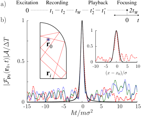
Figure 1: (color online). (a) TRM sequence. (b) Reconstructed signal scaled with $\mathcal{A}/\Delta T$ at the emission point $\mathbf{r}_{0}$, close to the refocusing time $t=0$, for the shown billiard. The thick solid is the semiclassical prediction (Eq. (13)). Numerical simulations for various $\Delta T$ and $\mathcal{A}$: $5000$ and $150\times 300$ (blue dotted), $10000$ and $150\times 300$ (green dashed), and $5000$ and $300\times 600$ (red dash-dotted). Right inset: reconstructed signal at $t=0$ close to $\mathbf{r}_{0}$ from the semiclassical prediction (solid) and simulation (red dash-dotted) with $\Delta T=5000$ and $\mathcal{A}=300\times 600$.

In Fig. 1(b) we show the numerical results for the time dependence on the reconstructed signal at $\mathbf{r}_{0}$. The normalized $\mathcal{F}\mathcal{A}/\Delta T$ are well described by the semiclassical prediction (thick solid) confirming the scaling with $\Delta T$ and $\mathcal{A}$ of Eq. (8). The normalizing factor for the numerical results is approximately 1.4 times the semiclassical one. Such a difference may be due to our discretization of the quantum problem as well as the difficulties of the diagonal approximation to recover exact numerical values. The signal-to-noise ratio does not change appreciably when the recording time is doubled, while it is improved by increasing $\mathcal{A}$. In the right inset we show the spatial reconstruction of the wave-packet around $\mathbf{r}_{0}$ for the refocusing time $t=0$. We see that the semiclassical prediction (thick solid) provides the proper scaling behavior and, up to the normalization factor, a quantitative description of the TRM results.

The numerical implementation of TRM for integrable geometries results in a refocusing that strongly depends on the position of the transducers and with a signal hardly distinguishable from the background. The semiclassical approach allows to understand this important difference between chaotic and integrable systems. In the former the exponential proliferation of trajectories allows to encode the information at all times, while in the latter the registered signal will be strongly dependent on whether or not the source and the transducer are connected by a stable trajectory.

Experimentally, the TRM procedure has been shown to be robust against local and global perturbations introduced between the recording and injection phases cit-Derode . Even in the absence of these perturbations, it is natural to expect that in any TRM setup the environment acting during the re-emission is slightly modified respect to that of the recording phase. In the same spirit of the LE studies, we can model this situation by assuming that in the recording process we have a Hamiltonian $H$ that determines $G(\mathbf{r}_{i},\mathbf{r}^{\prime},\tau)$ in Eq. (1), while a modified $\tilde{G}(\mathbf{r},\mathbf{r}_{i},t+\tau)$ is governed by the slightly different Hamiltonian $\tilde{H}$. For the LE the details of the perturbation $\tilde{H}-H$ are not important, and its effect can be accounted, after some averaging, by affecting the contribution of each trajectory $s$ by an additional factor $\exp[-L_{\hat{s}}/2\tilde{l}]$, where $\tilde{l}$ is an effective mean-free-path associated to the perturbation. In general $\tilde{l}$ depends on the velocity of the particle, i.e. for perturbations modeled by an auxiliary impurity potential characterized by a strength $\gamma$ we have $1/\tilde{l}=\gamma\tau^{2}/L_{\hat{s}}^{2}$ cit-Jalabert . Including this $\tau$-dependent phase prevents us of using the ergodic approach, but working along the lines of Eqs. (7)-(9) we obtain a maximum refocusing for a non-static environment given by

$$\mathcal{F}_{\mathrm{max}}(\gamma)= \frac{2\mathcal{V}}{\sqrt{\pi}\sigma\mathcal{A}\gamma}\int_{0}^{\infty}\mathrm{d}\eta\ \eta^{2}\exp[-\eta^{2}]$$

$$\times\left(\exp\left[-\frac{\gamma L_{1}}{\eta\mathcal{V}^{2}}\right]-\exp\left[-\frac{\gamma L_{2}}{\eta\mathcal{V}^{2}}\right]\right),$$ (14)

which reduces to $\mathcal{F}_{\mathrm{max}}\left(1-(t_{2}+t_{1})/4\tilde{\tau}\right)$ for $t_{2}~{}\ll~{}\tilde{\tau}$; to $\mathcal{F}_{\mathrm{max}}\exp{\left[-(t_{2}+t_{1})/4\tilde{\tau}\right]}$ for $t_{2}\!-\!t_{1}~{}\ll~{}\tilde{\tau}$; and to $c\tilde{\tau}/(\sqrt{\pi}\sigma\mathcal{A})\exp{\left[-c^{\prime}t_{1}/2\tilde{\tau}\right]}$ for $t_{2}\!>\!\tilde{\tau}$. The numerical constants $c=2.94$ and $c^{\prime}=0.46$ are given by rational-argument values of the $\Gamma$ function, and the characteristic time is defined as $\tilde{\tau}=\mathcal{V}/(2\sqrt{\pi}\gamma)$. The proportionality of the reconstructed signal with the injection interval is clearly lost in the limit of $t_{2}\!>\!\tilde{\tau}$ since the perturbation renders ineffective the longest recording times. From the relevant limits that we have singled out, the second one is the most important for current experiments. It has a Fermi-Golden-Rule structure that can be obtained under very general considerations. For perturbations where the effective elastic mean-free-path $\tilde{l}$ increases with the Lyapunov exponent of the unperturbed system (i.e. mass distortion in a Lorentz gas cit-Jalabert ) the characteristic time $\tilde{\tau}$ increases with the chaoticity of the system. Similarly to the Fermi-Golden-Rule regime of the LE, such a motional narrowing effect translates into larger stability, and improved refocalization, for the more chaotic systems, in agreement with the experimental findings cit-Derode .

In summary, we have described the refocalization signal for the time reversal mirror procedure through the semiclassical approximation. The chaotic nature of the underlying classical dynamics appears as a key ingredient to ensure the stability of the refocalization towards perturbations and the proportionality of the recovered signal with the injection time.

We thank T. Kramer and K. Richter for valuable discussions and A. Goussev for helpful correspondence. We acknowledge financial support of the French-Argentinian program ECOS-Sud and the Deutsche Forschungsgemeinschaft within FG 760. RAJ acknowledges the hospitality of the Universität Regensburg and HMP that of the ICTP of Trieste and the MPI-PKS of Dresden.

References

- (1) E. L. Hahn, Phys. Rev. 80, 580 (1950).
- (2) S. Zhang, B.H. Meier and R.R. Ernst, Phys. Rev. Lett. 69, 2149 (1992).
- (3) A. Derode, P. Roux and M. Fink, Phys. Rev. Lett. 75, 4206 (1995); M. Fink, Phys. Scr. T90, 268 (2001).
- (4) C. Draeger and M. Fink, Phys. Rev. Lett. 79, 407 (1997).
- (5) S. Catheline et al., Phys. Rev. Lett. 100, 064301 (2008); G. Montaldo et al., Wave Random Complex 17, 67 (2007).
- (6) G. Lerosey et al., Phys. Rev. Lett. 92, 193904 (2004).
- (7) P.R. Levstein, G. Usaj and H.M. Pastawski, J. Chem. Phys. 108, 2718 (1998); H.M. Pastawski et al., Physica A (Amsterdam) 283, 166 (2000).
- (8) A. Peres, Phys. Rev. A 30, 1610 (1984).
- (9) R.A. Jalabert and H.M. Pastawski, Phys. Rev. Lett. 86, 2490 (2001); F.M. Cucchietti, H.M. Pastawski and R.A. Jalabert, Phys. Rev. B 70, 035311 (2004).
- (10) T. Gorin et al., Phys. Rep. 435, 33 (2006).
- (11) H.M. Pastawski et al., Europhys. Lett. 77, 40001 (2007).
- (12) G. Bal and L. Ryzhik, SIAM J. App. Math. 63, 1475 (2003).
- (13) J. de Rosny et al., Phys. Rev. E 70, 046601 (2004).
- (14) C. Bardos and M. Fink, Asymptotic Analysis 29, 157 (2002).
- (15) R.K. Snieder and J.A. Scales, Phys. Rev. E 58, 5668 (1998).
- (16) G. Tanner and N. Søndergaard, J. Phys. A 40, R443 (2007).
- (17) M. Brack and R.K. Bhaduri, Semiclassical Physics, (Addison-Wesley, Reading, MA, 1997).
- (18) A. Goussev et al., New J. Phys. 10, 093010 (2008).
- (19) M. Sieber, J. Phys. A 32, 7679 (1999).
- (20) A. Goussev, private communication.
- (21) N. Argaman, Phys. Rev. B 53, 7035 (1996).