Hyperbolicity and the effective dimension of spatially-extended dissipative systems

Abstract

Using covariant Lyapunov vectors, we reveal a split of the tangent space of standard models of one-dimensional dissipative spatiotemporal chaos: a finite extensive set of $N$ dynamically entangled vectors with frequent common tangencies describes all the physically relevant dynamics and is hyperbolically separated from possibly infinitely many isolated modes representing trivial, exponentially decaying perturbations. We argue that $N$ can be interpreted as the number of effective degrees of freedom, which has to be taken into account in numerical integration and control issues.

Nonlinear dissipative partial differential equations (PDEs) are ubiquitous in the description of pattern-forming, chaotic, and turbulent systems Cross_Hohenberg-RMP1993 . Even though they are formally infinite-dimensional dynamical systems, it is now well accepted that their chaotic solutions evolve in an effective manifold of finite dimension. For many generic PDEs such as the Kuramoto-Sivashinsky (KS) and the complex Ginzburg-Landau (CGL), it is in fact proven that trajectories are first exponentially attracted to a finite-dimensional invariant manifold called the inertial manifold InertialManifold . This object, however, remains largely formal, as there does not exist a constructive way of determining of which modes it is composed. Similarly, trajectories eventually fall into a global attractor of finite Hausdorff dimension. For large systems, this dimension, as well as other quantities measuring the amount of chaos in the system, can be estimated via the calculation of Lyapunov exponents. These dimensions remain, however, global quantifiers. One approach to determine which modes actually compose and contribute to the dynamics is that pursued, e.g., by Cvitanovic et al. UPOExpansion , but it is difficult and limited to rather small systems.

A related difficulty lies in the numerical integration of dissipative PDEs (which remains the primary way of studying their often chaotic solutions). If the finite-dimensionality of their attractors justifies that a numerical study is possible at all, there is no a priori criterion to define the minimal resolution for a faithful simulation, and in practice, one typically checks the convergence of results upon increasing the resolution.

In this Letter, we use covariant Lyapunov vectors (CLVs), recently made numerically accessible thanks to an efficient algorithm Ginelli_etal-PRL2007 , to show that the tangent dynamics of large KS and CGL systems is essentially characterized by a well-defined set of “physical” modes. Because the covariant vectors span the intrinsic (Oseledec) subspaces corresponding to each Lyapunov exponent, and thus allow access to hyperbolicity properties, we are able to show that the physical modes are decoupled from the remaining set of hyperbolically “isolated” degrees of freedom. In the context of dissipative partial differential equations, our results imply that a faithful numerical integration needs to incorporate at least as many degrees of freedom as the number of such physical modes and that further increasing the resolution increases the number of degrees of freedom associated with the trivially decaying isolated modes.

We first focus on the one-dimensional KS equation, taken here as a prototypical dissipative PDE showing space-time chaos Cross_Hohenberg-RMP1993 ; Chate-ScholarPedia . It governs a real field $u(x,t)$ according to

$$\partial_{t}u=-\partial_{x}^{2}u-\partial_{x}^{4}u-u\partial_{x}u,~{}~{}~{}~{}x\in[0,L].$$ (1)

Figure 1 shows the Lyapunov spectrum for a fixed system size $L=96$ but different spatial resolutions and periodic or rigid boundary conditions (PBC or RBC) Algorithm . The spectrum consists of two parts: first a smooth region of positive, zero, and some negative exponents, then a rather steep region of negative exponents arranged in steps of two for PBC. The two regions are separated by an abrupt change in slope (bottom inset). Remarkably, the spectra for different spatial resolutions overlap with the extra exponents coming from the higher resolution simply accumulating in the second region, at the negative end of the spectrum (upward and downward triangles). Thus the threshold index separating the two regions stays unchanged (here around $j=40$) upon increasing resolution. Note also that the boundary conditions only change the multiplicity of modes in the second region, where every other mode is exactly the same for both PBC and RBC.

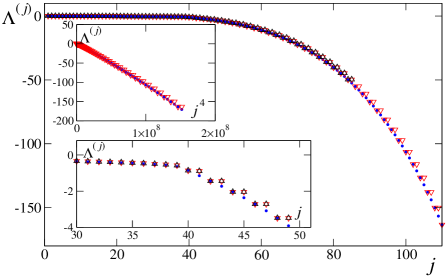
Figure 1: (color online) Lyapunov spectrum $\Lambda^{(j)}$ made of exponents arranged by decreasing value for the one-dimensional KS equation with $L=96$. Black upward triangles: $k_{\rm cut}=42\cdot 2\pi/L$ and PBC. Red downward triangles: $k_{\rm cut}=85\cdot 2\pi/L$ and PBC. Blue dots: $k_{\rm cut}=170\cdot\pi/L$ and RBC ($u(L,t)=u(0,t)=0$). In all three cases the spectrum yields a positive region with maximum Lyapunov exponent $\Lambda^{(1)}\approx 0.09$. Top inset: $\Lambda^{(j)}$ vs $j^{4}$ for the large-$j$ (isolated) modes. Bottom inset: close-up around the threshold.

The above observations suggest that modes in the second region, hereafter called “isolated”, for reasons given below, are residual, highly damped degrees of freedom not necessary to describe properly the essential dynamics. In contrast, the modes in the first region, which should be intimately associated with phase space dynamics, will be called “physical”. In the following, we substantiate this intuition on a rigorous basis studying the CLVs associated with Lyapunov exponents. The CLVs for the isolated modes, contrary to those of the physical modes, possess an approximately sinusoidal, delocalized structure as can be seen from their power spectra (Fig. 2b), as well as directly from their rather uneventful spatiotemporal evolution (Fig. 2a). With PBC, the two modes forming a step show the same dominant wavenumber with an arbitrary phase shift. This is not the case of RBC where the phase of the sinusoidal structure is fixed at the boundary. The peak wavenumber $k_{\rm peak}^{(j)}$, which linearly increases with $j$ (top panel of Fig. 2c), is in fact just the $j$-th wavenumber allowed in the given spatial geometry (multiplicity taken into account): $k_{\rm peak}^{(j)}=[j/2]\cdot 2\pi/L$. For large-enough $j$, $\Lambda^{(j)}\sim-(k_{\rm peak}^{(j)})^{4}\sim-j^{4}$ (top inset of Fig. 1), which indicates that the values of the Lyapunov exponents of the isolated modes are governed by the stabilizing linear term of the KS equation (i.e. the fourth-order derivative).

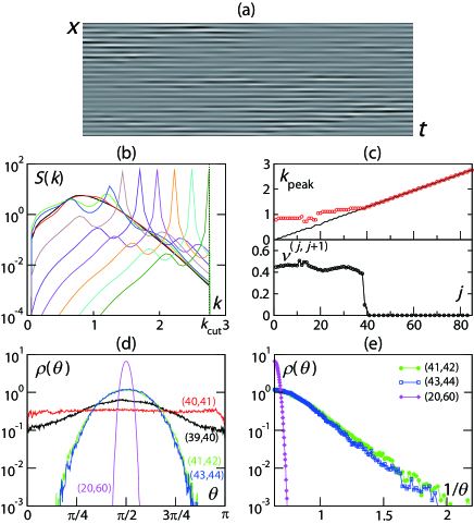
Figure 2: (color online). Properties of CLVs for the KS system ($L=96$, $k_{\rm cut}=42\cdot 2\pi/L$, and PBC). (a) Spatiotemporal plot of a typical vector in the isolated region ($j=46$, total time $100$). (b) Spatial power spectra of vectors of indices $j=1$, $16$, $32$, $38$, $44$, $52$, $60$, $68$, $76$, $84$ (from left to right in peak position). (c) Top panel: peak wavenumber in the power spectra (red circles) and $k=[j/2]\cdot 2\pi/L$ (black line). Bottom panel: DOS violation fraction $\nu^{(j,j+1)}_{\tau}$ for pairs of neighboring vectors (pairs within the same step are omitted). (d) Angle distributions between pairs of vectors. (e) Same as (d) but with a different abscissa.

The sinusoidal structure of the isolated modes indicates that they are nearly orthogonal to each other. Indeed, distributions of the angle $\theta$ between pairs of CLVs of indices $j\geq 42$ are peaked at $\pi/2$ and drop rapidly near $0$ and $\pi$. This is also true if only one of the vectors is taken in the region $j\leq 41$, but for any pair of vectors taken from this region, the angle distribution spans the whole $[0,\pi]$ interval (Fig. 2d). A careful analysis of the angle distributions reveals that those involving isolated modes seem to have an essential singularity near $0$ (and $\pi$): $\rho(\theta)\sim\exp(-\text{const.}/\theta)$ (Fig. 2e). Given the sharpness of this behavior, we cannot conclude about the possibility for these distributions to be strictly bounded away from zero. The above results determine accurately the threshold at $j=41$, and therefore the number of physical modes, and give the precise definition of physical and isolated modes: contrary to the physical modes, the isolated modes do not have any tangencies with other isolated modes (except the partner in the same step) nor with physical modes. They can be said to be “hyperbolically isolated.”

The absence of tangency for isolated modes can be confirmed from another viewpoint, that of the so-called domination of the Oseledec splitting (DOS) DOS , which quantifies, loosely speaking, the degree of dynamical isolation of the Oseledec subspaces from each other due to the strict ordering of Lyapunov exponents. Let $\lambda_{\tau}^{(j)}(t)$ be the finite-time Lyapunov exponent averaged over a period $\tau$ around time $t$. The splitting of the space formed by the vectors associated with the modes $j_{1}$ and $j_{2}(>j_{1})$ is said to be dominated if $\lambda_{\tau}^{(j_{1})}(t)>\lambda_{\tau}^{(j_{2})}(t)$ holds for all $t$ with $\tau$ larger than some finite $\tau_{0}$. It is mathematically proven that DOS implies absence of tangency between the Oseledec subspaces, or the CLVs DOS . To quantify DOS, we define, following Yang_Radons-PRL2008 $\Delta\lambda_{\tau}^{(j_{1},j_{2})}(t)\equiv\lambda_{\tau}^{(j_{\rm min})}(t)-\lambda_{\tau}^{(j_{\rm max})}(t)$ with $j_{\rm max}\equiv\max(j_{1},j_{2})$ and $j_{\rm min}\equiv\min(j_{1},j_{2})$ and measure the time fraction of DOS violation $\nu^{(j_{1},j_{2})}_{\tau}=\langle\Theta(\Delta\lambda_{\tau}^{(j_{1},j_{2})}(t))\rangle$, where $\Theta(z)$ is the step function and $\langle\cdots\rangle$ denotes the time average. The result is shown in the bottom panel of Fig. 2c for pairs of neighboring exponents: $\nu^{(j,j+1)}_{\tau}$ with $\tau=0.2$ drops sharply near the threshold and becomes strictly zero for $j\geq 41$. In fact, $\nu^{(j,j^{\prime})}_{\tau}$ stays zero for any pairs with $j$ or $j^{\prime}>41$, though in some cases slightly larger values of $\tau$ are required. This confirms the absence of tangencies of the isolated modes, already seen from the angle distributions, and the number of physical modes.

We now turn our attention to a different case in order to test the validity of our results beyond the simple KS equation. Let us consider the CGL equation, whose universal relevance and genericity is now well-established Cross_Hohenberg-RMP1993 ; Aranson_Kramer-RMP2002 . In one space dimension, it governs a complex field $W(x,t)$ according to:

$$\partial_{t}W=W-(1+i\beta)|W|^{2}W+(1+i\alpha)\partial_{x}^{2}W\;.$$ (2)

In the following we consider a so-called “amplitude turbulence” regime Shraiman_etal-PhysD1992 , i.e. a strongly chaotic regime where amplitude and phase modes evolve on rather short time- and length-scales. (Results for other regimes, such as phase turbulence, will be presented elsewhere TBP .) Specifically, we use $\alpha=-2.0,\beta=3.0,L=64$, and PBC.

For sufficiently high spatial resolution, the Lyapunov spectrum indeed shows an isolated, stepwise region as for the KS equation (Fig. 3c), but here the multiplicity of each step is four and the spatiotemporal evolution of isolated modes reveal patches of traveling waves (Fig. 3ab). (The effects of spatial resolution and/or boundary conditions are also similar to our observations on the KS equation.) As for the KS equation, this is in agreement with the linear stability analysis: normal modes are traveling waves of the form $\exp[i(\pm kx-\omega_{k}t)+\Lambda t]$ with $\Lambda=1-k^{2}$ and $\omega_{k}=\alpha k^{2}$. Indeed, the values of the Lyapunov exponents in the isolated region behave like this and the vectors are composed of traveling waves propagating at a velocity of $\pm\omega/k$. Compared to the KS case, the additional multiplicity of two comes from the degeneracy between $k$ and $-k$ modes. Moreover, this degeneracy implies that these two modes are in fact mixed up in a single vector: isolated vectors are either in the pure $k$ mode (Fig. 3a), in the pure $-k$ mode, or patches of the two (Fig. 3b).

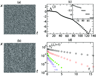
Figure 3: (color online) CGL equation in the amplitude turbulence regime ($L=64$, $k_{\rm cut}=31\cdot 2\pi/L$, and PBC). (a,b) Spatiotemporal plots of the phase component of a typical vector $j=91$ in the isolated region (same trajectory, but at two distant periods of time, during a total time of $20$ for each plot). (c) Lyapunov spectrum; inset: close-up around threshold. (d) Time fraction $\nu^{(j,j+1)}_{\tau}$ of DOS violation, as a function of $\tau$ ($j=78$, 82, 86, 90, 94, from top to bottom).

In spite of these differences, the isolated modes for CGL remain dynamically isolated from any other mode. Although $\nu^{(j,j+1)}_{\tau}$ measured with small $\tau$ is not zero in the isolated region, a clear threshold is found when considering larger $\tau$ values: Contrary to what happens for $j_{1},j_{2}\leq 86$, all $\nu^{(j_{1},j_{2})}_{\tau}$ for $j_{2}\geq 87$ show a decrease faster than exponential, indicating the existence of a finite $\tau$ beyond which $\nu^{(j_{1},j_{2})}_{\tau}$ is zero (Fig. 3d). Consequently, we can also define the isolated modes by their DOS as for the KS equation, and determine exactly the number of physical modes (here at $j=86$). Indeed, physical modes have no tangencies with any isolated modes ($j\geq 87$). Moreover, angle distributions involving isolated modes show, like for the KS equation, the essential singularity $\sim\exp(-\text{const.}/\theta)$ near tangency.

We now discuss our results. We first note that the threshold separating physical from isolated modes does not coincide with the appearance of steps in the Lyapunov spectrum (for PBC). Lyapunov exponents alone can only provide a good guess: For the KS and CGL systems treated above, the first steps start respectively at $j=40$ and $j=79$, whereas the exact thresholds are at $j=41$ and $j=86$. Indeed, a closer scrutiny of the exponents reveal that the first steps are actually not perfect.

Let us now specify the implication of the lack of tangencies for the isolated modes. Suppose that we add to the dynamics an infinitesimal perturbation along the CLVs of some isolated modes. Then this perturbation decays exponentially to zero as indicated by their negative Lyapunov exponents, and the absence of tangencies implies that this does not induce any perturbation along directions spanned by the other Lyapunov modes. In contrast, perturbations along physical modes will propagate to other physical modes through tangencies between them, and could eventually induce activity in the modes associated with positive exponents, growing to considerably affect phase space dynamics even if the initial perturbation was made in the direction associated with negative exponents. In this sense, the dynamics corresponding to the physical modes is highly entangled, but completely decoupled from the decaying dynamics of the isolated modes. Therefore, all the degrees of freedom associated with physical modes are necessary to faithfully describe phase space dynamics, while adding further more degrees of freedom associated with isolated modes does not affect phase space dynamics in any significant way. The number of physical modes scales linearly with the system size $L$: rescaled Lyapunov spectra collapse both in the physical and in the isolated region with the stepwise structure retained (Fig. 4). In particular, the dimension density defined from the number of physical modes is larger than others, for instance being almost twice the Kaplan-Yorke dimension KY (inset of Fig. 4). It is therefore natural to interpret the number of physical modes as an embedding dimension of the global attractor. Furthermore, we speculate, pending mathematical rigor, that the number of physical modes could be related to the dimension of the inertial manifold, which is a positively invariant and exponentially attracting smooth manifold embedding the global attractor (the subspace spanned by the physical modes would then be the local linear approximation of the inertial manifold IM2 ). While this conjecture would drastically lower existing estimates for the dimension of the KS inertial manifold $D\leq\text{const.}\times L^{2.46}$ IM2 , it is however in line with the extensivity of chaos already observed in the past for the same models Manneville-LNP1985 ; Egolf .

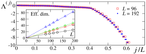
Figure 4: (color online). Extensivity of the Lyapunov spectrum for the KS equation with PBC. Inset: quantities indicating effective dimensions of the system: number of non-negative exponents (circles), Kaplan-Yorke dimension (squares), metric entropy (diamonds, multiplied by $50$), and number of physical modes (triangles).

Our results suggest that a faithful numerical integration of PDEs needs to incorporate at least the degrees of freedom associated with all physical modes. Moreover, the extensivity of the number of physical modes implies that the minimal resolution evaluated in systems of moderate size carries over to arbitrarily large system size $L$. Our obtained number of effective degrees of freedom would also be helpful to determine the minimal number of constraints necessary for a full control of a continuum system, with applications to real situations like e.g. the suppression of ventricular fibrillation.

In summary, we have shown, using Lyapunov analysis, that the tangent space of two representative nonlinear dissipative PDEs systems can be divided into two parts: a finite dimensional manifold spanned by strongly interacting physical modes, and the remaining set of isolated, strongly damped modes. We demonstrated that isolated modes are hyperbolically separated from all other modes, and thus satisfy the property of domination of Oseledec splitting. Similar results were obtained also for a chain of diffusively-coupled tent maps (not shown, TBP ). We have interpreted the number of physical modes as an embedding dimension of the global attractor. The extensivity of this dimension could also be of interest in view of the studies by Egolf et al. Egolf arguing about the “building blocks” of spatiotemporal chaos. We hope our results will trigger work to clarify these issues at the mathematical level, as much as numerical investigations of other dissipative systems, like those yielding fully developed turbulence, for which no rigorous proofs are known about the existence of an inertial manifold. Besides their theoretical importance, our results are also useful for the numerical integration and control issues of dissipative PDEs.

References

- (1) M. C. Cross and P. C. Hohenberg, Rev. Mod. Phys. 65, 851 (1993).
- (2) For a review, see J.C. Robinson, Chaos 5, 330 (1995).
- (3) Y. Lan and P. Cvitanović, arXiv:0804.2474.
- (4) F. Ginelli et al., Phys. Rev. Lett. 99, 130601 (2007).
- (5) H. Chaté and Y. Kuramoto, “The Kuramoto-Sivashinsky equation”, Scholarpedia (to be published).
- (6) A spectral method with discrete Fourier or sine transform up to a cutoff wavenumber is used in order to avoid aliasing. Time is integrated using the operator-splitting method with a time step . Data are typically recorded over a period of after a transient of .
- (7) C. Pugh, M. Shub, and A. Starkov, Bull. Am. Math. Soc. 41, 1 (2004); J. Bochi and M. Viana, Ann. Math. 161, 1423 (2005).
- (8) H. L. Yang and G. Radons, Phys. Rev. Lett. 100, 024101 (2008).
- (9) I. S. Aranson and L. Kramer, Rev. Mod. Phys. 74, 99 (2002).
- (10) B. I. Shraiman et al., Physica 57D, 241 (1992).
- (11) K. A. Takeuchi et al. (to be published).
- (12) J.-P. Eckmann and D. Ruelle, Rev. Mod. Phys. 57, 617 (1985).
- (13) J.C. Robinson, Phys. Lett. A 184, 190 (1994); M.S. Jolly, R. Rosa, and R. Temam, Adv. Diff. Eq. 5, 31 (2000).
- (14) P. Manneville, in Macroscopic Modelling of Turbulent Flows, Lecture Notes in Physics Vol. 230, edited by U. Frisch et al., (Springer-Verlag, Berlin, 1985), p. 319.
- (15) D. A. Egolf and H. S. Greenside, Nature (London) 369, 129 (1994); M. P. Fishman and D. A. Egolf, Phys. Rev. Lett. 96, 054103 (2006).