The memory kernel of the self-intermediate scattering function on a MD-simulated glass-forming Ni₂₀Zr₈₀-system

Abstract

The memory kernel of the self-part of the intermediate scattering function is studied. We found that the short-time behavior of the memory kernel for our MD-simulated glass-forming Ni₂₀Zr₈₀-system shows a deviation from the polynomial form predicted by MCT. By using the gaussian approximation we give a more detailed description of the short-time dynamics of the system.

I INTRODUCTION

At present the phenomena behind the liquid-glass transition and the nature of the glassy state are not fully understood, despite the progresses of recent years. In contrast to usual phase transformations the glass transition seems to be primarily dynamic in origin and therefore new theoretical approaches have to be developed for its description. Several theoretical models have been proposed to explain the transition and the corresponding experimental data. The latter concern of both the temperature dependence of particular properties, such as the shear viscosity and the structural relaxation time, and the time dependence repsonse of the spectra as visible in the dielectric susceptibility, inelastic neutron scattering, and light scattering spectra investigations. The spectral measurements have been extended to cover the large frequency range from below the primary $\alpha$-relaxation peak up to the high-frequency region of microscopic dynamics dominated by vibrational modes Cum97 .

One of the promising approaches in this field is mode coupling theory (MCT). MCT originally was developed to model critical phenomena Kad ; Kawa . The non-classical behavior of the transport properties near the critical point was thought to be caused by nonlinear couplings between slow (hydrodynamics and order parameter) modes of the system. In later years, the MCT was found to be applicable more generally, to describe nonlinear effects in dense liquids Ernst and nonhydrodynamic effects in the case of the glass transition.

The idealized schematic model of the MCT for the liquid-glass transition, firstly proposed by Bengtzelius et.al. Bengt84 and independently by Leutheusser Leuth84 , implies that the liquid (”ergodic”) state is characterized through a decay of structural correlations while below a critical temperature $T_{c}$ a solidlike (”nonergodic”) state exists with structural arrest where fluctuations are effectively frozen. In this state correlations decay on a longer time scale by thermally activated diffusion processes Das ; Gotze ; Sjorgen .

According to the MCT the time dependence of the correlation functions for structural fluctuations follows from a damped harmonic oscillator equation with a retarted damping term. All the details concerning the time evolution of the structural correlations are hidden in the memory kernel that describes the retarted damping.

In a previous paper Tei96E , hereafter refered to as I, one of us has evaluated this memory kernel from the time dependence of the correlation functions in the molecular dynamics(MD) simulations of the glass-forming Ni₅₀Zr₅₀-system. Here two results from I shall be recalled: first, it found that the short-time behavior of the memory kernel of the self-part of the intermediate scattering function $\Phi(q,t)$ shows a deviation from the polynomial form commonly assumed in the idealized(or extended) schematic model of the MCT. This deviation, in particular, explains the absence of the inverse powerlaw decay of the correlation predicted by the MCT. The deviations originate from the vibrational motions of the atoms in local potential minima and are restricted to the short times, below some 0.3 ps. This, on the other hand, explains that the MCT predictions for the late $\beta$-regime and for the $\alpha$-peak are in a good agreement with the experimental results Mez ; Kieb ; Dian ; Cum92 ; Meg and MD-simulation Kob ; Lew . Second, there is a characteristic quantity $g_{m}$, as introduced in Tei96L , that can be used as a relative measure to describe how close a liquid structure has approached the arrested nonergodic state. If $g_{m}>1$ for a given temperature $T$, then the system is able to undergo the transition into an idealized nonergodic state with a structural arrest; if $g_{m}<1$, the system remains in the (undercooled) liquid state ($T>T_{c}$), and if $g_{m}\approx 1$, the system stands in a critical situation.

The behavior of the memory kernel $F(t)$ and the parameter $g_{m}$ are formally related through the characteristic function $g(\Phi)=F(t)(1/\Phi(q,t)-1)$ introduced in Tei96L . $g_{m}$ means the maximum of $g(\Phi)$ for $\Phi\in[0,1]$ and the short time behavior of $F(t)$ is, in particular, visible in the behavior of $g(\Phi)$ for values $\Phi(q,t)\rightarrow 1$. Therefore we here are interested in a detailed description of $g(\Phi)$ for short times, respectively $\Phi(q,t)\rightarrow 1$. Since, according to I, $\Phi(q,t)$ for short times is determined by the vibration spectrum of the amorphous structure, the memory kernel $F(t)$ for short times and the corresponding $g$ also depend on the vibration spectrum. The latter is visible in the velocity autocorrelation function (VACF) and thus we in the following look for an interrelationship between the VACF and $g$. Moreover, we here consider the Ni_1-xZr_x system at $x=0.8$, while in I the concentration $x=0.5$ was investigated. Thus we ask to which extend the results for $x=0.8$ confirm the results for $x=0.5$ from I.

Our paper is organized as follows: In Section II, we present the model and give some details of the computations. Section III gives a brief discussion of some aspects of the mode coupling theory as used here and it describes the gaussian approximation to relate $\Phi(q,t)$ and the VACF at the short time. Results of our MD-simulations and their analysis are then presented and discussed in Section IV.

II SIMULATIONS

As in paper I, the present simulations are carried out as state-of-the-art isothermal-isobaric ($N,T,p$) calculations. The Newtonian equations of $N=$ 648 atoms (130 Ni and 518 Zr) are numerically integrated by a fifth order predictor-corrector algorithm with time step $\Delta t$ = 2.5x10^-15s in a cubic volume with periodic boundary conditions and variable box length L. With regard to the electron theoretical description of the interatomic potentials in transition metal alloys by Hausleitner and Hafner Haus we model the interatomic couplings as in Tei92 by a volume dependent electron-gas term $E_{vol}(V)$ and pair potentials $\phi(r)$ adapted to the equilibrium distance, depth, width, and zero of the Hausleitner-Hafner potentials Haus for Ni₂₀Zr₈₀ MUT . For this model simulations were started through heating a starting configuration up to 2000 K, yielding a homogeneous liquid state. The system then is cooled continuously to various annealing temperatures with cooling rate $-\partial T$ = 1.5x10¹² K/s. Afterwards the obtained configurations of various annealing temperatures (here 1500-800 K) are relaxed by modelling an additional isothermal annealing that depend on the object temperature. Finally the time evolution of these relaxed configurations is modelled and analyzed. Full details of the simulations are given in MUT .

III THEORY

III.1 Mode Coupling Theory

In the MCT equation of motion for the correlation function of structural fluctuations with wave vector $\mathbf{q}$ can be expressed as a damped harmonic oscillator equation (see, e.g, Gotze85 ; Gotze88 )

$$\ddot{\Phi}(q,t)/\Omega_{0}^{2}+\Phi(q,t)+\int_{0}^{t}d\tau F(q,t-\tau)\dot{\Phi}(q,\tau)=0$$ (1)

with initial conditions $\Phi(q,0)=1$ and $\dot{\Phi}(q,0)=0$. $\Omega_{0}$ is a microscopic (phonon) frequency and $F(t)$ is the memory kernel. The schematic modell assumes that the time dependence of $F(q,t)$ can be expressed by that of $\Phi_{q}(t)$ and the idealized version of MCT, neglecting atomic diffusion, relies on the assumption

$$F(q,t)=F_{0}(t):=h(t)+f(\Phi(q,t))$$ (2)

where $f(\Phi)$ means the polynomial in $\Phi$ and $h(t)$ a short time viscous damping which conveniently is approximated by an instantaneous term $\eta_{0}\delta(t)$. The asymptotic behavior of $\Phi(q,t)$ is determined by $f(\Phi)$.

As mentioned above, there is for a given temperature a characteristic function $g(\Phi)$ whose maximum value can be used to determine whether the system is able to undergo a structural arrest ( $g_{m}>1$) or whether it remains in the (undercooled) liquid state ( $g_{m}<1$ ). This characteristic function can be derived as follows: Given $\lim\limits_{t\rightarrow\infty}\Phi\approx\Phi^{\infty}>0$. Let us assume that there is a critical time $t_{c}$ so that for $t>t_{c}$

$$\dot{\Phi}(t)=0\>,$$ (3)

$$\ddot{\Phi}(t)=0\>.$$ (4)

Substitute the equations (3) and (4) in MCT-Eq. (1), then the MCT-Eq. becomes

$$\Phi^{\infty}+f(\Phi^{\infty})(\Phi^{\infty}-1)=0,$$ (5)

and after a little algebra we find

$$g(\Phi)=f(\Phi)(1/\Phi-1)$$ (6)

with $\Phi\in\left[0,1\right]$. This function is related in simple way to $\Delta F(\Phi)=f(\Phi)-\Phi/(1-\Phi)$ frequently used in the schematic MCT GoHaus .

According to the extended version of MCT which simulates atomic diffusion by taking into account the coupling to transverse currents, the memory kernel has the following form

$$F(t)=\mathcal{L}^{-1}\{1/[D(z)+\frac{1}{\mathcal{L}({F_{0}(t)})_{z}}]\}$$ (7)

Here $\mathcal{L}$ means the Laplace transform, $\mathcal{L}^{-1}$ its inverse. $D(z)$ models the coupling to the transverse currents. $F(t)$ from Eq.(7) leads to the final decay of structural fluctuations also below $T_{c}$. This sets one of the basic problems in classification of the solutions of Eq.(1) as it may not be obvious for a given solution whether it belongs to the regime above or below $T_{c}$ if atomic diffusion is included.

For our analysis we introduce the Laplace Transform for the memory kernel $F(t)$ and the correlation function $\Phi(t)$, by taking $z=\varepsilon-i\omega$ with $\varepsilon\rightarrow 0$, as follows

$$\lim_{\varepsilon\rightarrow 0}\mathcal{L}\{F(t)\}_{\varepsilon-i\omega} = F_{c}(\omega)+iF_{s}(\omega)$$ (8)

$$\lim_{\varepsilon\rightarrow 0}\mathcal{L}\{\Phi(t)\}_{\varepsilon-i\omega} = \Phi_{c}(\omega)+i\Phi_{s}(\omega)$$ (9)

where $\Phi_{c}(\omega)$ and $\Phi_{s}(\omega)$ are the cosines-part and sinus-part of the Fourier transformed $\Phi(t)$. It should be noted that according to the fluctuation-dissipation theorem the loss part of the dynamic susceptibility spectrum $\chi^{\prime\prime}(\omega)$ is related to the dynamics structure factor $\Phi_{c}(\omega)$ via

$$\chi^{\prime\prime}(\omega)=\omega\Phi_{c}(\omega)$$ (10)

Substitute equations (8) and (9) in MCT-Eq. (1), then we obtain the equation for the spectral distribution $\omega F_{c}(\omega)$ of the memory kernel

$$\omega F_{c}(\omega)=\frac{\omega\Phi_{c}(\omega)}{\left[1-\omega\Phi_{s}(\omega)\right]^{2}+\left[\omega\Phi_{c}(\omega)\right]^{2}}\>.$$ (11)

Taking the inverse-Fourier transformed $F_{c}(\omega)$, we have the time dependent memory kernel

$$F(t)=\frac{2}{\pi}\int_{0}^{\infty}d\omega F_{c}(\omega)\cos(\omega t)\>.$$ (12)

III.2 Gaussian Approximation

According to the theoretical models studied in the theory of liquids Boon ; Hansen ; Balucani we want to illustrate the correlation functions in the short-time regime for temperatures near the critical temperature. One of the models based on a cummulant expansion NiRah express the correlation function in an isotropic system

$$\Phi(q,t)=\exp\left\{-q^{2}\rho_{1}(t)+q^{4}\rho_{2}(t)-\ldots\right\},$$ (13)

where

$$\rho_{1}(t) = \frac{1}{6}\left\langle\left|\textbf{{x}}_{i}(t+t_{0}){-\textbf{x}}_{i}(t_{0})\right|^{2}\right\rangle\>,$$ (14)

$$\rho_{2}(t) = \frac{1}{2}\left[\rho_{1}(t)\right]^{2}\left[R_{2}(t)-1\right]\>,$$ (15)

$$R_{2}(t) = \frac{3}{5}\frac{\left\langle\left|\textbf{{x}}_{i}(t+t_{0})-\textbf{{x}}_{i}(t_{0})\right|^{4}\right\rangle}{\left[\left\langle\left|\textbf{{x}}_{i}(t+t_{0})-\textbf{{x}}_{i}(t_{0})\right|^{2}\right\rangle\right]^{2}}$$ (16)

The assumption that $\Phi(q,t)$ can be expressed only by the leading term of expansion Boon ; NiRah

$$\Phi(q,t)=\exp\left\{-\frac{q^{2}}{6}\left\langle\left|\mathbf{r}\mathnormal{(}t+t_{0})\mathbf{-r}\mathnormal{(}t_{0})\right|^{2}\right\rangle\right\}$$ (17)

is called the Gaussian approximation. Also in this approximation the correlation function is related to one-sixth the mean square displacement (MSD) of atoms during time $t$. In section IV. we will show our calculating results of Eq.(17) and prove that this approximation is correct in the short-time regime.

To show, by using this Gaussian approximation, whether our system in the short-time regime is a purely harmonic system or not, we need a relation between the mean squared displacement and the spectral distribution $Z(\omega)$ of the velocity autocorrelation function $Z(t)$ and a assumption that in purely harmonic system $Z(\omega)$ would be proportional to the density of state (DOS) $Z_{dos}(\omega)$. One find that relation

$$\left\langle\left|\mathbf{r}\mathnormal{(}t+t_{0})\mathbf{-r}\mathnormal{(}t_{0})\right|^{2}\right\rangle=6\omega_{0}^{2}\int_{0}^{\infty}d\omega\frac{(1-\cos(\omega t))}{\omega^{2}}Z(\omega)\>,$$ (18)

where

$$Z(\omega) = \int_{0}^{\infty}dt\cos(\omega t)Z(t)$$ (19)

$$= \int_{0}^{\infty}dt\cos(\omega t)\frac{\left\langle{v}_{i}(t+t_{0})\cdot{v}_{i}(t_{0})\right\rangle}{\left\langle\left|{v}_{i}(t_{0})\right|^{2}\right\rangle}\>,$$

$$\omega_{0}^{2} = \frac{1}{3}\left\langle\left|{v}_{i}(t_{0})\right|^{2}\right\rangle=\frac{k_{B}T}{M}$$ (20)

Actually Ngai et.al.(see e.g. RoNg ) have developed a model, which is called ”Coupling-Model”, in order to explain the dynamics of glass-forming liquids. Here we briefly review that model. The model made use of the assumption that vibration (phonon) and relaxation (diffusion) of the molecules contribute independently to the density-density correlation function; thus, $\Phi(q,t)$ is equal to the product $\Phi_{ph}(q,t)\times\Phi_{relax}(q,t)$ Zorn . In this model the correlation function of the relaxation $\Phi_{relax}(q,t)$

$$\Phi_{relax}(q,t)=\left\{\begin{array}[]{ll}\exp(-t/t_{0}(q,T))&\mbox{ for $t<t_{c}$}\\ \exp(-(t/\tau(q,T))^{1-n})&\mbox{ for $t>t_{c}$}\end{array},\right.$$ (21)

where respectively $t_{c}$ is a temperature-independent crossover time separating two time regimes in which the relaxation dynamics differ, $t_{0}$ the Debye-relaxation time, $\tau$ the Kohlrausch-relaxation time, and $1-n=\beta$ the Kohlrausch stretching exponent

The phonon contribution to $\Phi(q,t)$ is determined by the harmonic DOS of the phonon modes, $Z_{dos}^{harm}(\omega)$, according to the formula (see e.g.Zorn ; Lov ), in a classical limit,

$$\Phi_{ph}(q,t)=\exp(-\frac{q^{2}}{2}u(t,T))\>,$$ (22)

where

$$u(t,T)=\frac{2k_{B}T}{M}\int_{0}^{\infty}d\omega\frac{(1-\cos(\omega t))}{\omega^{2}}Z_{dos}^{harm}(\omega).$$ (23)

$u(t,T)$ decreases with time, leveling off to constant value $u(T)=\lim\limits_{t\rightarrow\infty}u(t,T)$. Correspondingly, $\Phi(q,t)$ has the value $\exp(-q^{2}u(T)/2)$, which is the well known Lamb-Mössbauer factor. For a single Einstein oscilator of frequency $\omega_{e}$ the harmonic DOS of the phonon modes is given by

$$Z_{dos}^{harm}(\omega)=\delta(\omega-\omega_{e})$$ (24)

and, for a Debye model of a solid,

$$Z_{dos}^{harm}(\omega)=\left\{\begin{array}[]{ll}3\omega^{2}/\omega_{D}^{3}&\mbox{for $\omega<\omega_{D}$}\\ 0&\mbox{for $\omega<\omega_{D}$}\end{array}\right.$$ (25)

By comparing this expressions of the coupling model with those of the theory of liquids and making a assumption that $Z_{dos}^{harm}(\omega)$ and $Z_{dos}(\omega)$ are the same quantities in the short-time regime we find that $\Phi_{ph}(q,t)$ (Eq.(22) with Eq.(23)) of the coupling model is the same as $\Phi(q,t)$ (Eq.(17) with Eq.(18)) of the theory of liquids (with the Gaussian approximation).

Considering that the model of the theory of liquid has a simple form we use for our further analysis that model. We believe that by making use of the model it is enough to prove whether in the short-time regime our system is a harmonic system or not.

Following Cummins et.al.Cum97 the correlation functions $\Phi(t)$ and the corresponding susceptibility spectrum $\chi^{\prime\prime}(\omega)$ can be considered to consist of three regimes: 1) at high frequencies (short times) a nearly temperature-independent microscopic structure; 2) at low frequencies (long times) a strongly temperature-dependent $\alpha$-relaxation peak associated with structural relaxation and diffusion process; 3) (intermediate frequencies) between a) and b) a minimum in $\chi^{\prime\prime}(\omega)$ (or ”plateau”) in $\Phi(t)$ whose amplitude and position is also temperature dependent.

From above definition of regions we write now in general form the full susceptibility spectrum

$$\chi^{\prime\prime}(T,\omega)=\chi_{st}^{\prime\prime}(T,\omega)+\chi_{it}^{\prime\prime}(T,\omega)+\chi_{lt}^{\prime\prime}(T,\omega)$$ (26)

After our intensive study about the short-time regime for the object temperatures near the critical temperature it is a little difficult to separate purely the short time regime from the intermediate regime. Also it is important to keep in mind that our definition for the short-time part in Eq.(26) include a small part of the $\beta$-relaxation process.

Considering that the spectral distribution of the velocity autocorrelation function $Z(t)$ for each temperature near $T_{c}$ ( from $\left[19\right]$ $T_{c}=1050\pm 25K$ ) shows too in our system a nearly temperature-independent form (see Fig. 1), we can scale now the short-time part of the susceptibility spectrum, so that

$$\chi_{sc}^{\prime\prime}(T,\omega)=\frac{T}{T_{0}}\chi_{M}^{\prime\prime}(\omega)\>,$$ (27)

where $\chi_{M}^{\prime\prime}$ is the master curve of the susceptibility spectrum that is now a temperature-independent quantity and is defined

$$\chi_{M}^{\prime\prime}(\omega)=\frac{1}{N}\sum_{i}^{N}\frac{T_{0}}{T_{i}}\chi_{st}^{\prime\prime}(T,\omega)\>,$$ (28)

where $N$ is the number of the object temperature and $T_{0}$ is a arbitrary normalization of temperature.

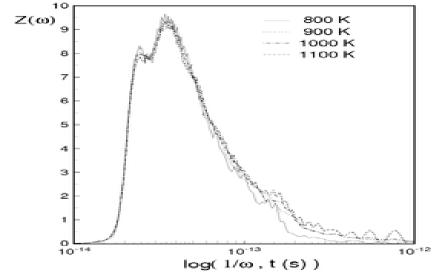
Figure 1: The spectral distribution of the velocity autocorrelation function for different temperature near $T_{c}$.

IV RESULTS AND DISCUSSION

The central object of our analysis is the self-part of the intermediate scattering function:

$$\Phi(\textbf{{q}},t)=\left\langle\exp\left\{i\textbf{{q}}\cdot[\textbf{{x}}_{i}(t+t_{0})-\textbf{{x}}_{i}(t_{0})]\right\}\right\rangle.$$ (29)

The bracket means averages over the atom $i$ and the initial configurations $t_{0}$.

In Figs. 2 and 3 we show the results evaluated from our MD data (with symbols) for wave vector $q=\frac{2\pi}{L}(n,0,0)$ with n = 8 and 6 which correspond respectively to $\left|q\right|=19.7$ nm^-1 and $\left|q\right|=14.7$ nm^-1. Both figures present the average over the star of six $q$ vectors which are equivalent on assuming equivalence of the simulation cube axis and their inverses.

IV.1 MCT-Analysis

The following Fig. 2 and 3 present the self-part of the intermediate scattering function for different object temperatures according to MCT (with line) and our MD-simulation (with symbols). The discrepancy between both results are considerable as results from the bad fitting of the Kohlrausch-law to our MD-data and the inaccurracy by calculation (see Tei96L ; Tei96E ; MUT for details of the algorithm used for calculation).

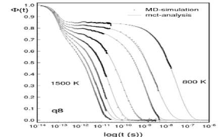
Figure 2: The self-part of the intermediate scattering function for wave vector $q_{8}$ from MD-data (with symbol) and from MCT-Equations (with line).

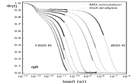
Figure 3: The same as Fig. 2 but for $q_{6}$.

From both figures we found that the self-part of the intermediate scattering function show for $q_{8}$ and $q_{6}$ at average temperatures the structural relaxations that happen in three succesive steps. According to predictions of the idealized schematic model of MCT the correlator should decay in three succesive steps [20] at this temperatures. The first is a fast initial decay on the time scale of vibrations of atoms ($t<1$ ps). This step is characterized by MCT only global. The second is the $\beta$-relaxation regime (typically in the range 1 ps $<t<$1 ns). In the early $\beta$-relaxation regime the correlator should decrease according to $\Phi(t)=f_{c}+A/t^{a}$ and in the late $\beta$-relaxation regime, which appear only in melting, according to von Schweidler-law $f_{c}-Bt^{b}.$ Between them the wide plateau appear near the critictical temperature $T_{c}$. In the case of idealized glass the von Schweidler-law does not appear more, but $\Phi(t)=f_{c}+A/t^{a}$ flows into the konstant asymptotic value $f_{c}$. In melting the $\alpha$-relaxation appear as the last step that results from the decay after the von Schweidler-law and could be described by the Kohlrausch-law $\Phi(t)=A_{0}\exp(-(t/\tau_{0})^{\beta})$ whose the relaxation time $\tau_{0}$ near the glass transition shifts dramatic to the longer time scale.

The decay for the early $\beta$-regime, which according to MCT follows the inverse power-law $\Phi\sim f_{c}+A/t^{a}$, could not be observed in our data. The reason for it is that in our system $\Phi_{m}(T)$ (the maximum of g$(\Phi)$) and $\Phi_{o}(T)$ (the threshold-value of $G(\Phi)$, see Eq.(33)) are nearly parallel, which cause that the power-law of the early $\beta$-regime is dressed up. On the one side, for this regime the so-called “Boson-peak” is discussed by several authors (see e.g.Sok ; Has ; Hab ), on the other side one called this peak as the $\beta$-maximun Mur95 . The first group of authors claimed that as a result of the atomic vibrations in the $\beta$-regime the boson-peak in a glass-system is observed, which depends on the fragility of the system. The more fragile the system ist, the weaker is the effects of the atomic vibrationen, i.e., the height of a boson-peak will be observed smaller and not clearer. As a result the relaxation-process is here observed clearer. In a connection with the fragility the glass-systems can be classified into two groups Angel ; Sok : 1) fragile glass-systems, which have no directional bonds, e.g., Van der Walls and ionic systems. These glass formers exhibit strong non-Arrhenius-like increase of the viscosity upon colling; 2) strong glass-systems, which have strong directional bonds. These glass-systems have the temperature dependence of the viscosity that is more Arrhenius like and weaker.

In a connection with this classification it is until today still difficult to determine whether the metallic-glass belongs to a strong glass-system or to a fragile glass-system, because usually the behavior of the viscosity in a metallic glass-system lies between both borderline case. So far from in hand analysis of our data we can state nothing about the “Boson-peak”.

We observed that the self-part of the intermediate scatteing function for $T<T_{c}$ shows a small bump at $t\approx 2.5x10^{-12}$ s. Th same phenomen war observed on MD-simulations for a OTP-system by Lewis and Wahnström Lew and for a binary Lenard-Jones mixture by Kob and Andersen Kob . This bump is interpreted by those authors as a result of the finite-size effect. The same bump was also observed on another Lenard-Jones mixture-system Wahn , on a liquid-salt system Sig , and on a colloidal-suspenstion system Low .

We have also analyzed that the height of plateaus as well as the time scale, at which the self-part of the intermediate scattering function decay finally to zero, depend strongly on wave vector $q$. Our MD-results of $\Phi(q,t)$ for the longer time show that $\Phi(q,t)$ always decay to zero at both $T<T_{c}$ and $T>T_{c}$. We interpret this result within the scope of the extended schematic MCT. The extended schematic MCT predicts that the long-time behavior of $\Phi(q,t)$ always decay to zero, when thermally activated hopping-processes is taken to be account in a system. According to Teichler Tei96E ; Tei96L ; Tei97 and Aspelmeier Timo95 these hopping-processes take place on a MD-simulated Ni₅₀Zr₅₀. As one can there observe, the reason for decaies of $\Phi(q,t)$ on the longer time scale is that on this time scale thermally activated hopping-processes run off. To prove this statement, we have to investigate the selft-diffusion konstant of atoms in our atoms. The MCT predicts that self-diffusion konstant follows a power-law that is a function of $T_{c}$:

$$D_{\alpha}\propto(T-T_{c})^{\gamma}$$ (30)

where $\gamma=1/(2a)+1/(2b)$ is valid and by knowing of the exponent $\lambda$ can be calculated. $\alpha$ is the specific atom. The estimation of $\gamma$ ove that expression is only possible, if a $q$-independence exponent $\lambda$ is given as required by deriving that expression. On MD-simulation we can determine for different temperatures of interest the self-diffusion konstant throught the calculation of mean squared displacement (MSD). Then we find the curve $D_{\alpha}$ vs $T$. The effective exponent ${\gamma}$ can be determine by using the least-squared method. From the curve we can prove whether the thermally activated hopping-processes run off at $T<T_{c}$ or tempertures near $T_{c}$ in our system or not, as we investigate whether there is a deviation from (30) or not. If there is this deviation, then it means that the hopping processes still take place at $T<T_{c}$ or $T$ near $T_{c}$ Tei97 ; HaYip .

From above discussion we can state that the behavior of $\Phi(q,t)$ in our system agree with the prediction of the extended MCT, in which the long-time behavior of $\Phi(q,t)$ decays to zero as a result of the atomic diffusion.

The MCT predicts that the behavior of $\Phi(q,t)$ in the last $\alpha$-regime can be good approximated by the Kohlrausch-law. We have determined the Kohlrausch’s parameters $A_{0}$, $\beta$, and $\tau_{0}$. Our results show that the parameter in our system (see Table 1) depends weakly on wave vectors $q$ and varies with temperature. The $\beta$-value increases with a decreasing $q$-value about 0.05. This result is similar as one by Lewis and Wahnström in MD-simulated OTP-system Lew .

On our results we have noticed that the $\beta$-value seem to increase to one at higher temperatures with a decreasing $q$-value. This phenomane is also found in another MD-simulation by Bernu et.al. Bernu . The MCT predicts that $\beta$-value for $q\sim q_{0}$ ($\sim$ 20 nm^-1), which corresponds to a nearest-neighbor distance, is found typically in range 0.6 $<\beta<$ 0.8 that depends on the system of interest; for $q\ll q_{0}$ the $\beta$-value seem to increase. Also our $\beta$-value agrees well with the MCT”s predictions.

According to MCT the $\alpha$-relaxation time diverge near $T_{c}$ after the power-law GoSRP ; HaYip

$$\tau_{0}(T)\propto(T-T_{c})^{\gamma}$$ (31)

where $\gamma$ is the same exponent in Eq.(30). On our results we have found that the behavior of the power-law was broken in the nearest environments from $T_{c}$, because as a result of thermally activated atomic diffusion the $\alpha$-relaxation time $\tau_{0}$ kept to a finite-value.

Through a viewing of the $\alpha$-relaxation time $\tau_{0}$ we have found that this relaxation time has a strong depending on $q$-value. The same result was observed in a MD-simulated binary Lenard-Jones mixture by Kob and Andersen Kob and in a experimentel quasy-elastic neutron scaterring on three polymers by Colmenero et.al. Col . We have noticed that there is an anomaly on the $\alpha$-relaxation time, namely, the relaxation time increases drastic near the glass-transition. One explains this anomaly TeiUv95 : the system is found above $T_{c}$ on the way to a metastable equilibrium of undercooled liquid-phases. Then the system comes below $T_{c}$ into a unstable state, where the relaxation processes take place in a direction of the equilibrium. On grounds of this anomaly we can state that the glass transition actually is a dynamic transition which is more in the change of the art on atomic movements and less in the change of the structure Roux ; Timo95

Figures 4 and  5 present the dynamic susceptibility. From both figures we found that there are three different frequency-regimes of the dynamics susceptibility as mentioned in theory section. As predicted by extended MCT the $\alpha$-peak shift with a decreasing temperature to the lower frequency, und this peak and the minimum of the dynamics susceptibility are no more dissapear at temperature near $T_{c}$. The extended MCT assumes this behavior, when thermally activited hopping-processes are included formally in the memory kernel $F(t)$. These processes has taken place in our system, i.e., these predictions agree with statements mentioned above.

Table 1: The Kohlrausch parameters $A_{0}$, $\tau_{0}$, $\beta$ fitted to $\Phi(q,t)$ from MD-data for wave vector $q_{8}$ and $q_{6}$.

	$q_{8}=19.7$ [nm-1]			$q_{6}=14.7$ [nm-1]
$T$ [K]	$A_{0}$	$\tau_{0}$[ns]	$\beta$	$A_{0}$	$\tau_{0}$[ns]	$\beta$
1500	0.690	0.004	0.807	0.821	0.007	0.917
1400	0.729	0.007	0.820	0.827	0.011	0.821
1300	0.746	0.012	0.840	0.835	0.018	0.911
1200	0.759	0.024	0.780	0.859	0.042	0.781
1100	0.761	0.095	0.740	0.860	0.146	0.795
1000	0.790	0.966	0.748	0.859	$\sim$ 1.400	0.813
900	0.826	$\sim$ 2.448	0.680	0.894	$\sim$ 4.871	0.741
800	0.848	$\sim$ 31.100	0.756	0.911	$\sim$ 38.640	0.794

We have noticed that the height of $\alpha$-peak for each temperature depends strongly on $q$-value, namely, the height of $\alpha$-peak decreases with a increasing $q$-value. The microscopic (phonon)-regime as well as the height of this regime decreases with a decreasing both $q$-value and $T$. This result could be simply interpreted, if one takes into consideration the height of plateaus (the non-ergodicity parameter $f_{c}$) on the intermediate scattering function, which depends strongly on the $q$-value. Because the height of the $\alpha$-peak is proportional to the height of plateaus, and the microscopic-peak is proportional to $1-f_{c}$, then the above mentioned dependence of the both height-peaks results directly from the $q$-dependence non-ergodicity paramater.

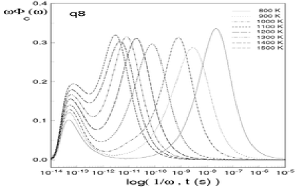
Figure 4: The dynamic susceptibility for wave vector $q_{8}$

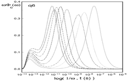
Figure 5: The same as Fig.  4, but for wave vector $q_{6}$

Figures  6 and  7 present our evaluated kernels $F(t)$ from MD-data of $\Phi(q,t)$ for both wave vectors of interest. From both figures we found that there is a temperature-dependence threshold-value $\Phi_{0}(T)$ ( $\Phi_{0}(T)\in[0;1]$ ), where under $\Phi_{0}(T)$ the behavior of $F(t)$ shows a course that corresponds to a polynom with positive coefficients, and otherwise this behavior deviats from a polynomial form. According to the prediction of the idealized MCT the kernel $F(t)$ as well as $f(\Phi)$ should show a polynomial form. Also our results do not agree with this prediction for all of regimes, but only for the regime that lies under $\Phi_{0}(T)$. This is understandable, because the idealized MCT does not fully describe the atomic vibrations of the system.

We have noticed that $\Phi_{0}(T)$ depends strongly on the $q$-value and weakly on the change of temperature. $\Phi_{0}(T)$ shift with a decreasing both $q$-value and $T$ to higher values.

There is here a important point that we can stretch, namely, by a calculating of the kernel $F(t)$ we can make for $\Phi(T)<\Phi_{0}(T)$ a new model of the memory kernel $f(\Phi)$, which presents of course a polynomial form. By a extending for $\Phi(T)>\Phi_{0}(T)$ we can then determine the term, which could be assigned to the atomic vibrations of the system and corresponds to the difference between the actually kernel $F(t)$ and the fitted memory kernel $f(\Phi)$. To this purpose we present our calculating for the kernel $F(t)$ as a function $\Phi$ in Fig.  8 and  9. According to MCT one define $f(\Phi)$ as follows :

$$f(\Phi)=\sum_{n}\lambda_{n}\Phi^{n}$$ (32)

where $\lambda_{n}$ are positive coefficients. We have fitted Eq.(32) to the kernel $F(\Phi)$. (see Fig. 10 and 11), and then we have for our system positive coefficients $\lambda_{n}$, which are given in Tables 2 and 3

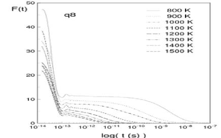
Figure 6: The kernel $F(t)$ for wave vector $q_{8}$.

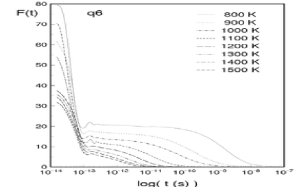
Figure 7: The same as Fig. 6 but for wave vector $q_{6}$.

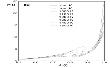
Figure 8: The kernel as a function of $\Phi$ for wave vector $q_{8}$.

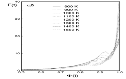
Figure 9: The same as Fig. 8 but for wave vector $q_{6}$.

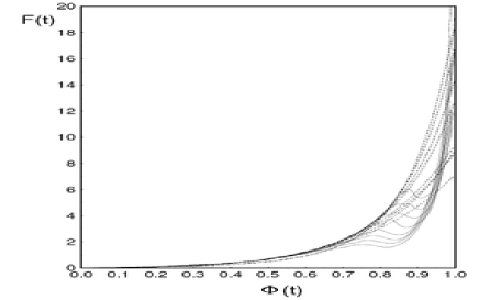
Figure 10: The kernel as function of $\Phi$ for wave vector $q_{8}$ (dotted line: extrapolated low-$\Phi$ polynomial).

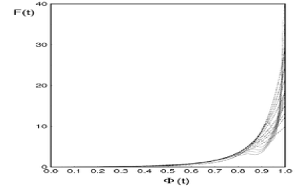
Figure 11: The same as Fig. 10 but for wave vector $q_{6}$.

Table 2: Coefficients of the polynomial expansion $f(\Phi)=\sum_{n}\lambda_{n}\Phi^{n}$ for wave vector $q_{8}$.

	$\lambda_{n}$
	$T$ K
$n$	$800$	$900$	$1000$	$1100$	$1200$	$1300$	$1400$	$1500$
1	0.255	0.423	0.232	0.357	0.271	0.253	0.308	0.198
2	0.714	0.794	0.658	0.688	0.661	0.598	0.820	0.800
3	0.040	0.597	1.757	1.177	1.174	1.630	1.165	1.592
4	1.390	1.318	2.144	1.621	2.089	1.850	1.876	2.628
5	2.218	1.930	1.637	1.655	2.535	2.116	1.439	0.057
6	1.586	1.628	0.700	1.817	2.414	1.828	0.593	1.769
7	0.321	0.621	0.000	1.445	0.232	0.566	0.742	0.040
8	0.000	0.000	0.009	1.251	0.012	0.000	2.089	0.185
9	2.438	1.575	1.552	0.623	0.032	0.000	0.002	0.143
10	9.864	8.069	5.907	2.253	0.040	0.020	0.000	0.451

Table 3: Coefficients of the polynomial expansion $f(\Phi)=\sum_{n}\lambda_{n}\Phi^{n}$ for wave vector $q_{6}$.

	$\lambda_{n}$
	$T$ K
$n$	$800$	$900$	$1000$	$1100$	$1200$	$1300$	$1400$	$1500$
1	0.235	0.316	0.362	0.246	0.173	0.189	0.240	0.162
2	0.021	0.386	0.373	0.246	0.394	0.278	0.394	0.135
3	0.918	0.924	0.990	0.965	0.214	0.612	0.682	0.515
4	1.291	0.994	1.240	1.006	0.529	0.810	0.640	1.397
5	0.016	0.588	0.873	0.127	1.448	1.323	1.563	2.250
6	0.102	0.130	0.289	0.009	2.594	2.528	2.250	4.494
7	0.001	0.000	0.000	1.780	3.493	2.873	2.756	0.689
8	0.000	0.249	0.366	4.877	3.671	4.101	1.277	0.185
9	0.001	1.238	1.893	6.649	2.645	0.563	1.166	0.063
10	0.000	3.152	5.013	2.365	0.020	0.003	0.003	0.001
11	3.192	7.167	10.157	0.092	0.030	0.303	1.323	0.003
12	8.222	7.978	0.002	0.044	0.042	0.005	0.001	0.014
13	15.148	1.400	0.000	0.013	0.011	0.002	0.002	0.000

To calculate Eq.(6), as in I, we introduce the following equations

$$G(\Phi):=F(\Phi)(1/\Phi-1)$$ (33)

$$g(\Phi)=P(\Phi)(1/\Phi-1)$$ (34)

Eq.(34) is analog to Eq.(6), where $f(\Phi)$ in $g(\Phi)$ is substituted by $P(\Phi)$. When we have calculated for $\Phi(T)<\Phi_{0}(T)$ $F(\Phi)$ as well as $f(\Phi)$, i.e., in compliance with both equations we also have calculated for $\Phi(T)<\Phi_{0}(T)$ the function $P(\Phi)$. Therefore we can now state that $P(\Phi)$ is also a polynomial function with positive coefficients $\lambda_{n}$, which will fit for $\Phi(T)<\Phi_{0}(T)$ the function $g(\Phi)$ to $G(\Phi)$.

In Figs. 12 and  13 we present the $G(\Phi)$-function. From both figures we can see that $G(\Phi)$ has a maximum at $\Phi_{0}(T)$. This maximum shifts with a decreasing $q$-value to a higher value. We can now fit the function $g(\Phi)$, which contains the polynomial function $P(\Phi)$ with positive coefficients (see Tables. 2 and  3), to $G(\Phi)$. Our results is shown in Figs.  14 and  15. From both figures we have for each temperature a maximum $g_{m}$ from $g(\Phi)$-function at $\Phi=\Phi_{m}$. This maximum is smaller als 1 for $T\geq 1100$ K ( $g_{m}<1$ ), and for $T\leq 1000$ K nearly equal 1 ( $g_{m}\approx 1$).

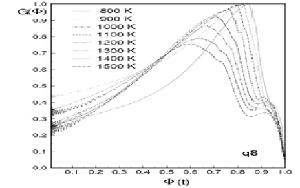
Figure 12: $G(\Phi)$ for wave vector $q_{8}$ according to Eq.(33).

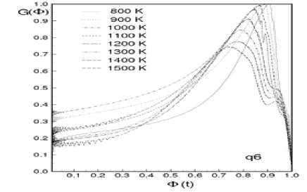
Figure 13: The same as Fig. 12 but for wave vector $q_{6}$.

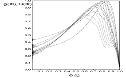
Figure 14: Fitting $g(\Phi)$ (dotted lines) to $G(\Phi)$ (full lines) for wave vector $q_{8}$ according to Eqs.(34) and (33).

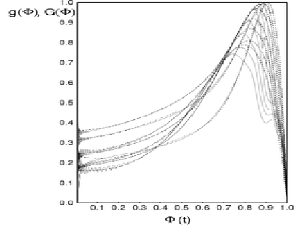
Figure 15: Fitting $g(\Phi)$ (dotted line) to $G(\Phi)$ (full lines) for wave vector $q_{6}$ according to Eqs.(34) and (33).

As mentioned in the theory section, $g_{m}$ describes a signature, so that, if $g_{m}<1$, the system is in a ergodic state (in a liquid state), and if $g_{m}>1$, it is in a non-ergodic state (in a structural arrest). Our results show that the Ni₂₀Zr₈₀-system is for $T\geq 1100$ K in a liquid state and for $T\leq 1000$ K nearly in a structural arrest with a correlation decay, which is as a result of a thermally activitated atomic diffusion. In Fig. 16 we present a curve $g_{m}$ vs $T$ for each $q$-value. From that Fig. one can see that our system has a critical temperature $T_{c}$ between 1000 K and 1100 K. Here we decide $T_{c}$ as about (1025 $\pm$ 25) K.

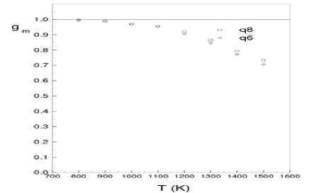
Figure 16: $g_{m}$ as a function of $T$.

IV.2 Gaussian Approximation

In following Figs. 17, 18, 19, and 20 we have calculated the self-part intermediate scattering function $\Phi(q,t)$ by using Gaussian approximation, also according to Eqs.(17) and (18). As input data for both equations are the mean squared displacement (MSD) and the velocity autocorrelations functions obtained from our MD-Data. From figures we found that the gaussian approximation is correct in the short-time regime, here also for $t<0.2$ ps. For $t>0.2$ ps the course of $\Phi(q,t)$ resulting from this approximation deviates from both MD-results and MCT-analysis-results. As mentioned in Subsection III.2 we have assumed that the DOS of phonons is equally approximated to the spectral distribution of velocity autocorrelations function (VACF). With this assumption we can state now that the phonon-regime in our system is the regime taken place in a range time smaller then 0.2 ps. This time is a nearly temperature-independent time.

Figure 17: The self-part of the intermediate scattering function for $T=$ 900 K, according to Eqs. (17)(line) and (18)(dotted line), MD-result (dotted - dashed line), MCT-analysis (dashed line).

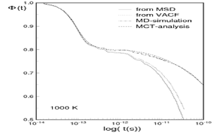
Figure 18: The same as Fig.17 but for $T=$ 1000 K.

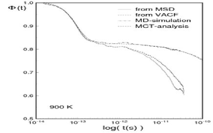
Figure 19: The same as Fig.17 but for $T=$ 1100 K.

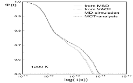
Figure 20: The same as Fig.17 but for $T=$ 1200 K.

To gain more our statement that this regime is as a result of the phonon vibrations we borrow a important relation of the liquid theory, namely, the relation between the spectral distribution of VACF and the susceptibility of the self-part intermediate scattering function $\Phi(q,t)$. According to theory that relation is approximated for a small $q$-value (lim $q\rightarrow 0$) as follows Boon ; Hansen

$$\chi^{\prime\prime}(\omega)=\omega\Phi_{c}(\omega)\approx q^{2}Z(\omega)/\omega$$ (35)

Fig.21 presents our calculating results of Eq.(35) with an assumption that our $q_{8}$-value is small enough. The calculating results show a fast nearly good agreement with that from the MCT-analysis (or a directly Fourier-tranformed $\Phi(q,t)$).

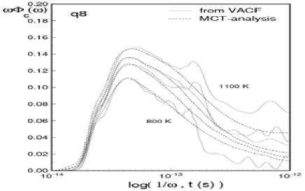
Figure 21: The susceptibility obtained from the spectral distribution of VACF through Eq.(35) (lines) and from the MCT-analysis (dashed lines)

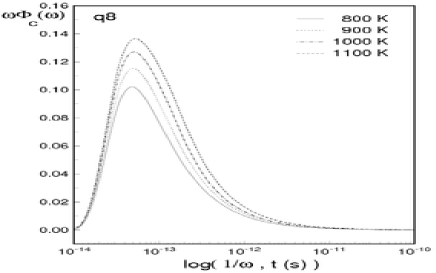
Figure 22: The susceptibility obtained before superposition for wave vector $q_{8}$.

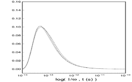
Figure 23: The susceptibility obtained after superposition.

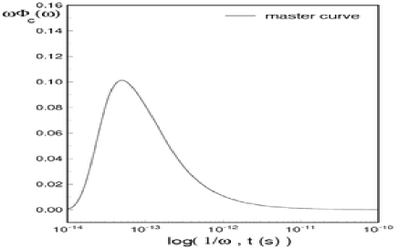
Figure 24: The master curve of the susceptibility for $q_{8}$ according to Eq.(28).

Figure 25: The new susceptibility after scaling for $q_{8}$ according to Eq.(27).

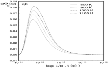
Figure 26: The susceptibility obtained before superposition for wave vector $q_{6}$.

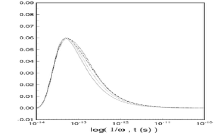
Figure 27: The susceptibility obtained after superposition.

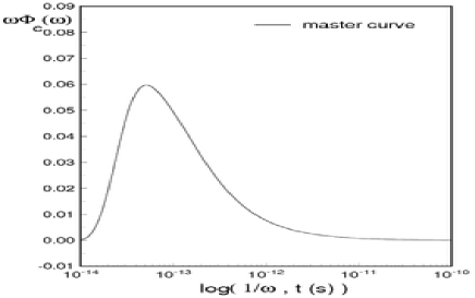
Figure 28: The master curve of the susceptibility for $q_{6}$ according to Eq.(28).

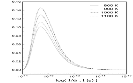
Figure 29: The new susceptibility after scaling for $q_{6}$ according to Eq.(27).

Actually we can do a inverse Fourier-transformation of the susceptibility obtained from Eq.(35) to find back the self-part intermediate scattering function $\Phi(q,t)$, but from the result shown in Fig.21 we do not do it, because Eq.(35) is a approximated relation that is really correct if the wave vector $q$ is very small (lim $q\rightarrow 0$ or, as one calls it, $q$ is in a hydrodynamics limit), and then if we attempt to back Fourier transform of its susceptibility, surely we can not find a better $\Phi(q,t)$ as it found through Eq.(18).

Further discussion about susceptibility we attempt to separate the susceptibility of this phonon-regime from the full susceptibility. As mentioned in Sec. III we assume that this separation is really to find a purely susceptibility of this regime. Our result for two wave vector is shown in Figs. 22 and 26. We scale now these susceptibilities, the result is shown in Figs.23 and 27, here we have chosen as a arbitrary normalization of temperature, $T_{0}$, 800 K, and we average these scaled susceptibilities through Eq.(3.14) to obtain the master curve of the susceptibility in this regime(see Figs.24 and 28). By using Eq.(27) we obtain the new susceptibility of this regime (see Figs. 25 and 29).

Adding the new susceptibility as shown in Figs.25 and 29 with the susceptibilities from other regimes, then we obtain the full susceptibility in the short-time regime as shown in Figs. 30 and 31. From both figures we found that the the peaks of the new full susceptibility for temperatures 1000 K and 1100 K are higher then those old ones, but that peaks for temperatures 800 K and 900 K are lower then those old ones.

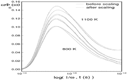
Figure 30: The full susceptibility before (dashed lines) and after scaling(full lines) in a short-time regime for wave vector $q_{8}$.

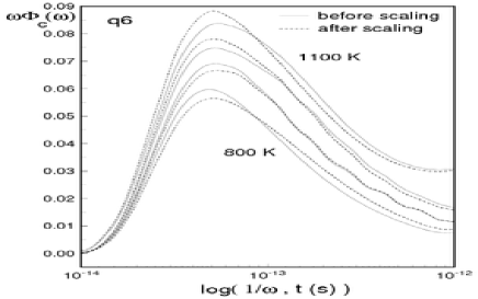
Figure 31: The full susceptibility before (dashed lines) and after scaling(full lines) in a short-time regime for wave vector $q_{6}$.

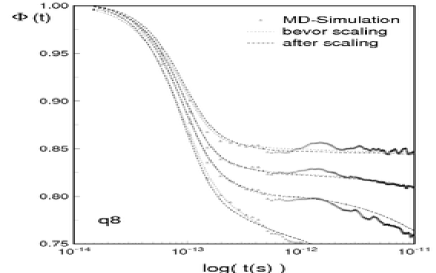
Figure 32: The self-part of the intermediate scattering function in a short-time regime, MD-results (Symbol), before (dotted line) and after scaling (dashed-line) for wave vector $q_{8}$.

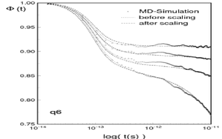
Figure 33: The self-part of the intermediate scattering function in a short-time regime, MD-results (Symbol), before (dotted line) and after scaling (dashed-line) for wave vector $q_{6}$.

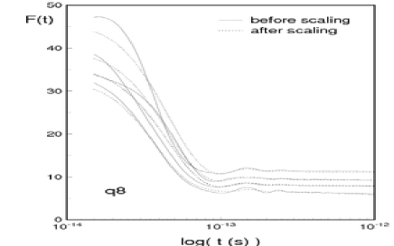
Figure 34: The kernel $F(t)$ in the short-time regime before (full lines) and after scaling (dotted lines) for wave vector $q_{8}$.

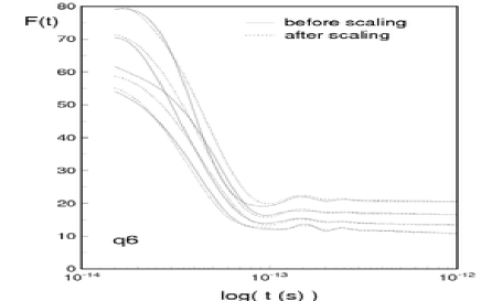
Figure 35: The kernel $F(t)$ in the short-time regime before (full lines) and after scaling (dotted lines) for wave vector $q_{6}$.

Taking back Fourier transformation of $\Phi_{c}(\omega)$ of the new full susceptibility in the short-time regime, then we obtain the new $\Phi(q,t)$ as shown in Figs. 32 and 33. The deviation of the new $\Phi(q,t)$ from the old one for each temperature of interest is taken place at a time range that is smaller then 0.5 ps.

It is interesting to calculate the new kernel $F(t)$ and the new $G(\Phi)$-function in this short-time regime. Our results for the kernel $F(t)$ are shown in Figs. 34 and 35. The new kernel $F(t)$ for each temperatures of interest show more regular then the old one. The deviation of the new kernel from the old one is taken place at a time range that is smaller then 0.5 ps, also this time range is the same as it found in the case of $\Phi(q,t)$. It is clear that $\Phi(q,t)$ in this regime depends strongly on the kernel $F(t)$.

V CONCLUDING REMARKS

Our system behaves as predicted by the schematic MCT-Modell, in the sense that the self-part intermediate scattering function $\Phi(q,t)$ shows at lower temperature three step of the structural relaxation. The behavior of the self-part intermediate scattering function $\Phi(q,t)$ agrees well for the long time with the prediction of the extended schematic MCT-Model in the sense that the self-part intermediate scattering function $\Phi(q,t)$ always decays to zero after long times as a result of thermally activated atomic diffusion.

The behavior of the memory kernel $F(t)$ agrees with the prediction of the extended MCT-Model in the sense that the behavior of $F(t)$ below $\Phi_{0}(t)$ corresponds to a polynomial function that has non-negative coefficients. This behavior depends strongly on the wave vector $q$.

As in I, to determine approximately the critical temperature $T_{c}$ we have used the maximum $g_{m}$ of the characteristic function $g(\Phi)$. We obtain $T_{c}\approx(1025\pm 25)$ K for our system.

Through the temperature superposition method in a short times regimes our results show that the vibration-phonon regime is really as a result of the harmonic phonon approximation, and then this regime can be good described by a gaussian approximation. In the case of a gaussian approximation, which follows from the liquid state theory, the courses of the self-part intermediate scattering function $\Phi(q,t)$ resulted from both VACF and MSD shows at time, $t\approx 0.5$ ps a deviation from the proper courses obtained from MD-simulations and MCT-analysis

- (1) H.Z. Cummins, G. Li, Y.H. Hwang, G.Q. Shen, W.M. Du, J. Hernandez, and N.J. Tao, Z.Phys. B 103, 501 (1997).
- (2) L.P. Kadanoff and J. Swift, Phys. Rev. 166, 89 (1968).
- (3) K. Kawasaki, Phys. Rev. 150, 1 (1966); Ann. Phys. (N.Y.) 61, 1 (1970).
- (4) M.H. Ernst and J.R. Dorfman, J. Stat. Phys. 12, 311 (1975).
- (5) U. Bengtzelius, W. Götze, and A. Sjölander, J. Phys. C 17, 5915 (1984).
- (6) E. Leutheusser, Phys. Rev. A 29, 2765 (1984).
- (7) P.S. Das and G.F. Mazenko, Phys. Rev. A 34, 2265 (1986).
- (8) W. Götze and L. Sjörgen, J. Phys. C 21, 3407 (1988).
- (9) L. Sjörgen, Z. Phys. B 79, 5 (1990).
- (10) H. Teichler, Phys. Rev. E 53, 4287 (1996).
- (11) F. Mezei, W. Knaak, and B. Farago, Phys. Rev. Lett. 58, 571 (1987); W. Knaak, F. Mezei, and B. Farago, Europhys. Lett. 7, 529 (1988)
- (12) M. Kiebel, E. Bartsch, O. Debus, F. Fujara, and H. Sillescu, Phys. Rev. E 45, 10301 (1992).
- (13) A. Fontana, F. Rocca, M.P. Fontana, B. Rosi, and A.J. Dianoux, Phys. Rev. B 41, 3778 (1990).
- (14) H.Z. Cummins, G. Li, M. Du, and A. Sakai, Phys. Rev. A 46, 3343 (1992).
- (15) W. van Megen and S.M. Underwood, Phys. Rev. E 49, 4206 (1994).
- (16) W. Kob and H.C. Andersen, Phys. Rev. E 51, 4626 (1995); ibid. 52, 4143 (1995).
- (17) L.J. Lewis and G. Wahnström, Phy. Rev E 50, 3865 (1994); L.J. Lewis, Phys. Rev. B 44, 4245 (1991).
- (18) H. Teichler, Phys. Rev. Lett. 76, 62(1996).
- (19) Ch. Hausleitner and Hafner, Phys. Rev. B 45, 128 (1992).
- (20) H. Teichler, Phys. Status Solidi B 172, 325 (1992).
- (21) A.B. Mutiara, Diplomarbeit, Göttingen (1996).
- (22) W. Götze, Z. Phys. B 60, 195 (1985).
- (23) G. Buchalla, U. Dersch, W. Götze and L. Sjörgen, J. Phys. C 23, 4239 (1988).
- (24) W. Götze and R. Haussmann, Z. Phys. B 72, 403 (1988).
- (25) B.J. Boon and S. Yip, Molecular Hydrodynamics, ( McGraw-Hill, 1980).
- (26) J.-P. Hansen and I.R. McDonald, Theory of Simple Liquids, 2nd Ed. ( Academic Press, London, 1986).
- (27) U. Balucani and M. Zoppi, Dynamics of the Liquid State, ( Clarendon Press, Oxford, 1994).
- (28) B.R.A. Nijboer and A. Rahman, Physica (Utrecht) 32, 415 (1966).
- (29) C.M. Roland and K.L. Ngai, J. Chem. Phys. 103, 1152 (1995).
- (30) R. Zorn, A. Arbe, J. Colmenero, B. Frick, D. Richter, and U. Buchenau, Phys. Rev. E 52, 781 (1995).
- (31) S.W. Lovesey, Theory of Neutron Scattering from Condensed Matter, Vol.1 ( Clarendon Press, Oxford, 1987).
- (32) A.P. Sokolov, E. Rössler, A. Kisliuk, and D. Quitmann, Phys. Rev. Lett. 73, 2062 (1993); E. Rössler, A.P. Sokolov, A. Kisliuk, and D. Quitmann, Phys. Rev. B 49, 14967 (1994).
- (33) A.K. Hasan, L. Börjesson, and L.M. Torell, J. Non-Cryst. Solids 172-174, 154 (1994).
- (34) J. Habasaki, I. Okada, and Y. Hiwatari, Phys. Rev. E 52, 2681 (1995).
- (35) T. Muranaka and Y. Hiwatari, Phys. Rev. E 51, 2735 (1995).
- (36) C.A. Angel, J. Non-Cryst. Solids 73, 1 (1985).
- (37) G. Wahnström, Phys. Rev. A 44, 3752 (1991).
- (38) G.F. Signorini, J,-L. Barrat, and M.L. Klein, J. Chem. Phys. 92, 1294 (1990).
- (39) H. Löwen, J.-P. Hansen, and J.-N. Roux, Phys. Rev. A 44, 1169 (1991).
- (40) H. Teichler, in: Simulationstechnicken in der Materialwissenschaft, edited by P. Klimanek and W. Pantleon (TU Bergakadamie, Freiberg, 1996).
- (41) T. Aspelmeier, Diplomarbeit, Göttingen (1995).
- (42) J.-P. Hansen and S. Yip, Transp. Theory Stat. Phys. 24, 1149 (1995).
- (43) B. Bernu, J.-P. Hansen, G. Pastore, and Y. Hiwatari, Phys. Rev A 36, 4891 (1987); ibid. 38, 454 (1988).
- (44) W. Götze and L. Sjörgen, Rep. Prog. Phys. 55, 241 (1992).
- (45) J. Colmenero, A. Arbe, A. Alegria, and K.L. Ngai, J. Non-Cryst. Solids 172-174, 229 (1994).
- (46) H. Teichler (unpublished).
- (47) J.-N. Roux, J.-L. Barrat, and J.-P. Hansen, J. Phys. Cond. Matt. 1, 7171 (1989).