Thomas-Fermi versus one- and two-dimensional regimes of a trapped dipolar Bose-Einstein condensate

Abstract

We derive the criteria for the Thomas-Fermi regime of a dipolar Bose-Einstein condensate in cigar, pancake and spherical geometries. This also naturally gives the criteria for the mean-field one- and two-dimensional regimes. Our predictions, including the Thomas-Fermi density profiles, are shown to be in excellent agreement with numerical solutions. Importantly, the anisotropy of the interactions has a profound effect on the Thomas-Fermi/low-dimensional criteria.

Introduction.

A Bose-Einstein condensate (BEC) is said to be in the Thomas-Fermi (TF) regime when the interaction energy dominates the zero-point energy TF_BEC ; p+sbook . Despite being a dilute gas, in this regime the BEC is strongly affected by interactions and behaves in a highly non-ideal manner. Furthermore, the TF description is relatively simple compared to full Gross-Pitaevskii theory and facilitates exact results p+sbook . Consider a BEC containing $N$ atoms of mass $m$ confined to a spherical harmonic trap $V(r)=m\omega^{2}r^{2}/2$, with harmonic oscillator (HO) length $l_{\mathrm{ho}}=\sqrt{\hbar/(m\omega)}$, and repulsive $s$-wave interactions with positive scattering length $a$. The TF regime occurs for large values of the parameter $Na/l_{\mathrm{ho}}$, and thus typically arises for dense strongly repulsive BECs.

Recently, a dipolar BEC was created with atomic dipoles polarized in a common direction by an external field griesmaier . Far from any scattering resonances the interaction can be represented by a pseudo-potential which includes the bare dipole-dipole interaction Yi ; Bohn ,

$$U(\mathbf{r})=g\delta({\bf r})+\frac{C_{\mathrm{dd}}}{4\pi}\,\hat{{\rm e}}_{i}\hat{{\rm e}}_{j}\frac{\left(\delta_{ij}-3\hat{r}_{i}\hat{r}_{j}\right)}{r^{3}}.$$ (1)

The first term describes s-wave scattering arising primarily from van der Waals interactions, where $g=4\pi\hbar^{2}a/m$. The second term describes the long-range part of the interaction between dipoles aligned along the unit vector $\hat{\mathbf{e}}$, where $C_{\rm dd}$ is the dipolar coupling strength. An important quantity is the ratio between the dipolar and s-wave interactions $\varepsilon_{\rm dd}=C_{\rm dd}/3g$ giovanazzi02 . For magnetic dipoles with moment $d$, $C_{\rm dd}=\mu_{0}d^{2}$, where $\mu_{0}$ is the permeability of free space. The signs and magnitudes of $C_{\rm dd}$ and $g$ can be controlled by rotation of the polarization axis giovanazzi02 , and by a Feshbach resonance Werner05 , respectively. A large range of $\varepsilon_{\rm dd}$ is therefore accessible and has already begun to be probed experimentally Werner05 ; koch ; lahaye .

In contrast to the van der Waals interaction, the dipolar interaction is long-range and anisotropic. This has dramatic consequences upon the behavior of a BEC and can even lead to collapse when $N$ and/or $C_{\rm dd}$ exceed critical values goral ; Santos00 ; Yi ; odell ; koch . Many properties of a dipolar BEC in the TF regime have already been discussed, e.g., its density profile odell , expansion dynamics stuhler , excitation frequencies odell ; giovanazzi2007 , rotation rickPRL and vortices odell07 . However, a systematic discussion of the criteria for the Thomas-Fermi regime of a dipolar BEC is currently lacking. In this paper we derive these criteria for the important cases of cigar-, pancake-, and spherically-shaped ground states. Our approach also reveals the criteria for the mean-field 1D and 2D regimes.

Theory.

At zero temperature the mean-field condensate wave function $\psi\equiv\psi({\bf r},t)$ obeys the Gross-Pitaevskii equation (GPE) p+sbook . Stationary solutions, for which $\psi$ is real, satisfy the time-independent GPE,

$$\left[-(\hbar^{2}/2m)\nabla^{2}+V({\bf r})+g\psi^{2}+\Phi_{\rm dd}({\bf r},t)\right]\psi=\mu\psi,$$ (2)

where $\mu$ is the chemical potential and the atomic density $n({\bf r})=\psi({\bf r})^{2}$ is normalised via $\int n({\bf r})d^{3}{\bf r}=N$.

We assume that confinement of the gas is provided by a cylindrically-symmetric harmonic trap $V({\bf r})=\frac{1}{2}m(\omega_{x}^{2}\rho^{2}+\omega_{z}^{2}z^{2})$, where $\omega_{x}$ and $\omega_{z}$ are the radial and axial trap frequencies, and $\rho=\sqrt{x^{2}+y^{2}}$. The s-wave interactions introduce a local mean-field potential $g\psi^{2}$ while the dipolar interactions introduce a non-local potential $\Phi_{\rm dd}$ given by Yi ,

$$\Phi_{\rm dd}({\bf r})=\int d^{3}{\bf r}^{\prime}U_{\rm dd}({\bf r}-{\bf r}^{\prime})\psi({\bf r}^{\prime})^{2},$$ (3)

where $U_{\rm dd}({\bf r})$ is the second term in Eq. (1).

In a time-dependent situation, where $\psi$ is complex, kinetic energy arises from both zero-point motion (density gradients) and velocities (phase gradients). However, in Eq. (2), only zero-point energy contributes. When this is negligible we enter the TF regime and Eq. (2) becomes,

$$gn({\bf r})+m(\omega_{x}^{2}\rho^{2}+\omega_{z}^{2}z^{2})/2+\Phi_{\rm dd}({\bf r})=\mu.$$ (4)

Equation (4) is satisfied by the well-known inverted parabola solution even in the presence of dipolar interactions odell . This has the form,

$$n({\bf r})=n_{0}\left[1-(\rho/R_{x})^{2}-(z/R_{z})^{2}\right],$$ (5)

where $n_{0}=15N/(8\pi R_{z}R_{x}^{2})$ is the peak density. The density is zero beyond the BEC boundary which is specified by the TF radii, $R_{x}$ and $R_{z}$. Expressions for $R_{x}$ and $R_{z}$ are presented in odell . For purely s-wave interactions, stable TF solutions only exist for repulsive interactions ($g>0$); under attractive interactions ($g<0$), the zero-point kinetic energy is crucial to stabilise the BEC against collapse. Additionally, the aspect ratio $\kappa=R_{x}/R_{z}$ equals the trap ratio $\gamma=\omega_{z}/\omega_{x}$, while for dipolar interactions this is not generally true.

It is useful to introduce a fictitious electrostatic potential $\phi({\bf r})=\int d{\bf r}^{\prime}n({\bf r})/(4\pi|{\bf r}-{\bf r}^{\prime}|)$. This satisfies Poisson’s equation $\nabla^{2}\phi=-n({\bf r})$. For dipoles aligned in the $z$-direction, $\Phi_{\rm dd}$ can then be expressed as odell ,

$$\Phi_{\rm dd}({\bf r})=-g\varepsilon_{\rm dd}\left[3\partial_{z}^{2}\phi({\bf r})+n({\bf r})\right].$$ (6)

Here the first term is anisotropic and long-range, while the second is short-range and contact-like. Note that the dipolar potential inside the inverted parabola (5) is odell ,

$$\Phi_{\rm dd}=\frac{n_{0}g\varepsilon_{\rm dd}}{R_{z}^{2}}\left[\frac{\rho^{2}}{\kappa^{2}}-2z^{2}-f(\kappa)\left(R_{z}^{2}-\frac{3}{2}\frac{\rho^{2}-2z^{2}}{\kappa^{2}-1}\right)\right],$$ (7)

where $f(\kappa)=(1+2\kappa^{2})/(1-\kappa^{2})-3\kappa^{2}{\rm atanh}\sqrt{1-\kappa^{2}}/(1-\kappa^{2})^{3/2}$ lies in the range $1\geq f(\kappa)\geq-2$ and $\kappa$ is determined by a transcendental equation Yi ; odell ,

$$3\kappa^{2}\varepsilon_{\rm dd}\left[\left(\frac{\gamma^{2}}{2}+1\right)\frac{f(\kappa)}{1-\kappa^{2}}-1\right]=(1-\varepsilon_{\rm dd})(\kappa^{2}-\gamma^{2}).$$ (8)

Cigar: 3D TF vs 1D mean-field.

Menotti and Stringari menotti analysed the crossover between the 3D TF and 1D mean-field regimes of a cigar-shaped s-wave BEC. We now extend their approach to include dipolar interactions. We begin by neglecting the axial trapping ($\omega_{z}=0$) and consider the BEC to be uniform along $z$ with 1D density (number of atoms per unit length) $n_{1}$. Then Eq. (6) reduces to the contact-like form,

$$\Phi_{\rm dd}(\mathbf{r})=-g\varepsilon_{\rm dd}n(\rho).$$ (9)

We can thus define an effective s-wave scattering length for the cigar $a_{\rm c}=a(1-\varepsilon_{\rm dd})$. The dipoles in the cigar lie predominantly end-to-end such that for $C_{\rm dd}>0$ ($C_{\rm dd}<0$) the net dipolar interaction is attractive (repulsive).

Introducing the dimensionless quantities $\rho^{\prime}=\rho/l_{x}$ and $\psi_{\rho}(\rho^{\prime})=l_{x}\psi(\rho)/\sqrt{n_{1}}$, where $l_{x}=\sqrt{\hbar/m\omega_{x}}$ is the radial HO length, Eq. (2) becomes,

$$\left(-\frac{\partial_{\rho^{\prime}}^{2}}{2}-\frac{\partial_{\rho^{\prime}}}{2\rho^{\prime}}+\frac{\rho^{\prime 2}}{2}+4\pi a_{\rm c}n_{1}{\psi_{\rho}}^{2}\right)\psi_{\rho}=\frac{\mu_{1}[a_{\rm c}n_{1}]}{\hbar\omega_{x}}\psi_{\rho}.$$ (10)

The chemical potential $\mu_{1}[a_{\rm c}n_{1}]$ is a function of $n_{1}$: one can numerically tabulate this equation of state by solving (10) for different values of $n_{1}$. The kinetic terms in Eq. (10) become negligible in comparison to the interaction terms when $a_{\rm c}n_{1}\gg 1$, in which case the TF radial density profile has the form,

$${\psi_{\rho}}^{2}=\frac{1}{4\pi a_{\rm c}n_{1}}\left(\frac{\mu_{1}[a_{\rm c}n_{1}]}{\hbar\omega_{x}}-\frac{1}{2}\rho^{\prime 2}\right),$$ (11)

with TF radius $R_{x}=\sqrt{2\mu_{1}[a_{\rm c}n_{1}]/\hbar\omega}$. Use of the normalisation condition $\int{\psi_{\rho}}^{2}2\pi\rho^{\prime}d\rho^{\prime}=1$ leads to the relation,

$$\mu_{1}[a_{\rm c}n_{1}]/\hbar\omega_{x}=2\sqrt{a_{\rm c}n_{1}}.$$ (12)

In the opposite regime of $a_{\rm c}n_{1}\ll 1$, termed the 1D mean-field regime p+sbook , the solution of Eq. (10) approximates the non-interacting radial HO state $\psi_{\rho}=\pi^{-1/2}e^{-\rho^{\prime 2}/2}$. Inserting this form into Eq. (2), we obtain the chemical potential perturbatively to be,

$$\mu_{1}[a_{\rm c}n_{1}]/\hbar\omega_{x}=1+2a_{\rm c}n_{1}.$$ (13)

We now wish to find the effect of finite axial trapping $\omega_{z}\neq 0$, for which $n_{1}(z)$ becomes inhomogeneous. We can easily estimate the correction to Eq. (9) using the TF result. Expansion of Eq. (7) as $\kappa\rightarrow 0$ cigar_expansions reveals that the leading correction is of order $\kappa^{2}$ and becomes negligible for $\kappa\ll 1$. Thus if the variation is sufficiently weak along $z$, Eq. (10) still defines the local chemical potential along $z$, $\mu_{1}[a_{\rm c}n_{1}(z)]$, and we can also employ the local density approximation,

$$\mu_{1}[a_{\rm c}n_{1}(z)]+m\omega_{z}^{2}z^{2}/2=\mu,$$ (14)

where $\mu$ is the global chemical potential of Eq (2). At the axial boundary $R_{z}$, this gives $\mu_{1}[a_{\rm c}n_{1}=0]+\frac{1}{2}m\omega_{z}^{2}R_{z}^{2}=\mu$. Then, by defining the function $\tilde{\mu}_{1}=(\mu_{1}[a_{\rm c}n_{1}(z)]-\mu_{1}[a_{\rm c}n_{1}=0])/\hbar\omega_{x}$, we can rewrite Eq. (14) as menotti ,

$$\tilde{\mu}_{1}[a_{\rm c}n_{1}(z)]=(\alpha^{2}/2)\left[1-(z/R_{z})^{2}\right]$$ (15)

where $\alpha=l_{x}R_{z}/l_{z}^{2}$. We can determine $n_{1}(z)$ by using the equation of state $\mu_{1}[a_{\rm c}n_{1}]$ to invert Eq. (15), i.e., $n_{1}(z)=\tilde{\mu}_{1}^{-1}[\tilde{\mu}_{1}[a_{\rm c}n_{1}(z)]]/a_{\rm c}$. For each choice of $\alpha$ we still need to know $R_{z}$, and this is obtained from the normalization condition $\int n_{1}(z)dz=N$ which can be written as,

$$\alpha\int^{1}_{-1}\tilde{\mu}_{1}^{-1}\left[\frac{1}{2}\alpha^{2}(1-\zeta^{2})\right]d\zeta=Na(1-\varepsilon_{\rm dd})\frac{l_{x}}{l_{z}^{2}},$$ (16)

where $\zeta=z/R_{z}$. On the right hand side we identify a natural dimensionless parameter. We enter the radial TF regime (and therefore the full 3D TF regime) when,

$$Na(1-\varepsilon_{\rm dd})l_{x}/l_{z}^{2}\gg 1.\quad\quad\mbox{3D TF cigar}$$ (17)

In this case we can use Eq. (12) to give the density profile,

$$n_{1}(z)=\frac{1}{a(1-\varepsilon_{\rm dd})}\left(\frac{l_{x}R_{z}}{2l_{z}^{2}}\right)^{4}\left(1-\frac{z^{2}}{R_{z}^{2}}\right)^{2},$$ (18)

where $R_{z}=[15Na(1-\varepsilon_{\rm dd})l_{z}^{8}/l_{x}^{4}]^{1/5}$. When $Na(1-\varepsilon_{\rm dd})l_{x}/l_{z}^{2}\ll 1$ we enter the 1D mean-field regime. Then, Eq. (13) leads to the density profile,

$$n_{1}(z)=\frac{1}{a(1-\varepsilon_{\rm dd})}\left(\frac{l_{x}R_{z}}{2l_{z}^{2}}\right)^{2}\left(1-\frac{z^{2}}{R_{z}^{2}}\right),$$ (19)

where $R_{z}=[3Na(1-\varepsilon_{\rm dd})l_{z}^{2}/l_{x}^{2}]^{1/3}$. Importantly, at $\varepsilon_{\rm dd}=1$ the overall contact interactions vanish and the TF cigar criterion (17) cannot be satisfied. When $\varepsilon_{\rm dd}=0$ we retrieve the results of menotti .

We now illustrate the key dependence on $\varepsilon_{\rm dd}$. We have obtained numerically the ground states of the 3D dipolar GPE, following the procedure outlined in goral02 . The axial density profiles for a cigar BEC are compared in Fig. (1) for various values of $\varepsilon_{\rm dd}$, according to the GPE (solid line), TF prediction (dashed line) and 1D mean-field prediction (dotted line). For weak dipolar interactions $\varepsilon_{\rm dd}=0.1$, giving $Na(1-\varepsilon_{\rm dd})l_{x}/l_{z}^{2}\gg 1$, the GPE profile is in excellent agreement with the 3D TF cigar prediction. For strong dipolar interactions $\varepsilon_{\rm dd}=0.8$, the 1D mean-field regime becomes an excellent description of the profile. For intermediate dipolar interactions $\varepsilon_{\rm dd}=0.5$ neither analytic form agrees well with the GPE results. In stuhler observations of the density and expansion of a cigar dipolar BEC were compared with TF predictions. For their parameters, including $\varepsilon_{\rm dd}\approx 0.16$ and $N\approx 5\times 10^{5}$, we obtain $Na(1-\varepsilon_{\rm dd})l_{x}/l_{z}^{2}\approx 50\gg 1$ thus satisfying the cigar TF criteria.

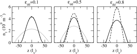
Figure 1: Axial density $n_{1}(z)$ of a cigar BEC for various values of $\varepsilon_{\rm dd}$ according to the GPE (solid lines), 3D TF cigar prediction of Eq. (18) (dashed line) and 1D mean field prediction of Eq. (19) (dotted line). We employ $Nal_{x}/l_{z}^{2}=100$, $\gamma=0.1$, $\omega_{x}=2\pi\times 50$Hz and ⁵²Cr atoms.

Pancake: 3D TF vs 2D mean-field.

We now consider a highly flattened pancake BEC and follow a similar methodology to the cigar BEC. We initially assume that the BEC has infinite radial extent and uniform 2D density $n_{2}$. Then, Poisson’s equation $\nabla^{2}\phi=-n({\bf r})$ reduces to $\partial_{z}^{2}\phi=-n(z)$, such that,

$$\Phi_{\rm dd}(\mathbf{r})=2g\varepsilon_{\rm dd}n(z),$$ (20)

This is, again, contact-like, giving an effective scattering length $a_{\rm p}=(1+2\varepsilon_{\rm dd})a$. In the pancake the dipoles are predominantly side-by-side and so the net interaction is repulsive (attractive) for $C_{\rm dd}>0$ ($C_{\rm dd}<0$). Introducing the dimensionless parameters $z^{\prime}=z/l_{z}$ and $\psi_{z}(z^{\prime})=\sqrt{l_{z}/n_{2}}\psi({\bf r})$, where $l_{z}=\sqrt{\hbar/m\omega_{z}}$ is the axial HO length, the GPE becomes,

$$\left(-\frac{\partial_{z^{\prime}}^{2}}{2}+\frac{z^{\prime 2}}{2}+4\pi a_{\rm p}l_{z}n_{2}\psi_{z}^{2}\right)\psi_{z}=\frac{\mu_{2}[a_{\rm p}l_{z}n_{2}]}{\hbar\omega_{z}}\psi_{z}.$$ (21)

The axial TF regime exists when $a_{\rm p}l_{z}n_{2}\gg 1$. By normalising the corresponding TF density profile via $\int\psi_{z}^{2}dz^{\prime}=1$, we obtain the TF chemical potential,

$$\mu_{2}[a_{\rm p}l_{z}n_{2}]/\hbar\omega_{z}=\left(6\pi a_{\rm p}l_{z}n_{2}\right)^{2/3}/2.$$ (22)

In the opposite regime of $a_{\rm p}l_{z}n_{2}\ll 1$, we enter the 2D mean-field regime. Here $\psi_{z}$ approximates the ground HO state $\psi_{z}=\pi^{-1/4}e^{-z^{\prime 2}/2}$ and the chemical potential is found perturbatively to be,

$$\mu_{2}[a_{\rm p}l_{z}n_{2}]/\hbar\omega_{z}=1+2\sqrt{2\pi}a_{\rm p}l_{z}n_{2}.$$ (23)

We now consider introduce finite radial trapping $\omega_{r}\neq 0$. Expanding Eq. (7) for $\kappa\rightarrow\infty$ pancake_expansions shows that the leading correction to Eq. (20) is of the order $\kappa^{-1}$ and negligible when $\kappa\gg 1$. Defining the function $\tilde{\mu}_{2}=(\mu_{2}[a_{\rm p}l_{z}n_{2}(z)]-\mu_{2}[a_{\rm p}l_{z}n_{2}=0])/\hbar\omega_{z}$ and employing the normalisation condition $\int n_{2}(\rho)2\pi\rho d\rho=N$ we obtain,

$$2\pi\beta^{2}\int^{1}_{0}\tilde{\mu}^{-1}\left[\frac{\beta^{2}}{2}(1-s^{2})\right]s~{}ds=\frac{Na(1+2\varepsilon_{\rm dd})l_{z}^{3}}{l_{x}^{4}},$$ (24)

where $s=\rho/R_{x}$ and $\beta=l_{z}R_{x}/l_{x}^{2}$. We therefore enter the axial TF regime, and hence the 3D TF regime, when,

$$Na(1+2\varepsilon_{\rm dd})l_{z}^{3}/l_{x}^{4}\gg 1.\quad\mbox{3D TF pancake}$$ (25)

For $\varepsilon_{\rm dd}=0$ we obtain the same result as in delgado . The corresponding 2D TF density profile is,

$$n_{2}(r)=\frac{1}{3\pi l_{z}a(1+2\varepsilon_{\rm dd})}\left(\frac{l_{z}R_{x}}{l_{x}^{2}}\right)^{3}\left(1-\frac{\rho^{2}}{R_{x}^{2}}\right)^{3/2},$$ (26)

where $R_{x}=[15Na(1+2\varepsilon_{\rm dd})l_{x}^{6}/l_{z}^{2}]^{1/5}$.

In the 2D mean-field regime of $Na(1+2\varepsilon_{\rm dd})l_{z}^{3}/l_{x}^{4}\ll 1$ we obtain,

$$n_{2}(r)=\frac{1}{\sqrt{2\pi}l_{z}a(1+2\varepsilon_{\rm dd})}\left(\frac{l_{z}R_{x}}{2l_{x}^{2}}\right)^{2}\left(1-\frac{\rho^{2}}{R_{x}^{2}}\right),$$ (27)

where $R_{x}=[16Na(1+2\varepsilon_{\rm dd})l_{x}^{4}/\sqrt{2\pi}l_{z}]^{1/4}$.

The experiment koch featured a pancake BEC with $\gamma=10$. For their parameters ($\omega_{x}=2\pi\times 330$, $N=25,000$ and $\varepsilon_{\rm dd}\approx 0.16$) we find $Na(1+2\varepsilon_{\rm dd})l_{z}^{3}/l_{x}^{4}=7$, suggesting that the initial BEC was not in the TF regime.

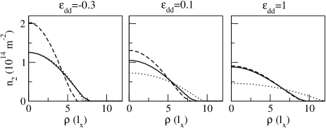
Figure 2: 2D density $n_{2}(\rho)$ of a pancake BEC for various values of $\varepsilon_{\rm dd}$ according to the GPE (solid lines), TF pancake prediction of Eq. (26) (dashed line) and 2D mean field prediction of Eq. (27) (dotted line). We employ $Nal_{z}^{3}/l_{x}^{4}=10$, $\gamma=10$, $\omega_{x}=2\pi\times 5$Hz and ⁵²Cr atoms.

In a very flat pancake, the net contact interactions become zero for $\varepsilon_{\rm dd}=-0.5$ and the TF regime cannot be supported. We demonstrate the role of $\varepsilon_{\rm dd}$ in Fig. 2 which presents the 2D density profile of a pancake BEC. For $\varepsilon_{\rm dd}=-0.3$, the net interactions are very weak and the 2D mean-field prediction (dotted line) agrees well with the GPE profile (solid line). Conversely, for $\varepsilon_{\rm dd}=1$ the combined interactions are relatively strong giving excellent agreement with the 3D TF prediction (dashed line). For an intermediate value of $\varepsilon_{\rm dd}=0.1$, the exact solution lies in between the two analytic predictions.

Approximately spherical BEC.

Away from the cigar and pancake limits $\Phi_{\rm dd}$ no longer reduces to a local interaction and we must consider its full form. In order to proceed we shall assume the validity of the 3D TF solution (5) and use energetic arguments to check its self-consistency. The combined s-wave and dipolar interaction energy for the TF solution is odell ,

$$E_{\rm i}=\int\left(\frac{g}{2}\psi^{4}+\Phi_{\rm dd}\psi^{2}\right)d^{3}{\bf r}=\frac{15N^{2}g\kappa}{28\pi R_{x}^{3}}\left[1-f(\kappa)\varepsilon_{\rm dd}\right]$$ (28)

We observe that when $\varepsilon_{\rm dd}=1/f(\kappa)$ the net interactions vanish and the TF regime cannot be achieved. The kinetic energy of a spherical TF distribution is $E_{\rm k}\approx 5N\hbar^{2}/2mR_{x}^{2}$, up to a logarithmic correction p+sbook . The TF approximation is valid when $E_{\rm i}/E_{\rm k}\gg 1$ which, using the above expressions and dropping the numerical prefactors ($\approx 1$), becomes $(Na\kappa/R_{x})\left[1-f(\kappa)\varepsilon_{\rm dd}\right]\gg 1$. From Eq. (8) we find that a spherical ($\kappa=1$) BEC occurs when $\varepsilon_{\rm dd}=\varepsilon_{\rm dd}^{0}$ where $\varepsilon_{\rm dd}^{0}=(5/2)(\gamma^{2}-1)(\gamma^{2}+2)$. Introducing the parameter $\delta=\varepsilon_{\rm dd}-\varepsilon_{\rm dd}^{0}$ and expanding Eq. (8) to first order in $\delta$ and $(\kappa-1)$, we obtain the relation $\kappa=1-(7\delta/15)(\gamma^{2}+2)^{2}/(12\gamma^{2}-2\gamma^{4}-3)$. Furthermore, we expand the expression for $R_{x}$ in odell and $f(\kappa)$ spherical_expansions . To first order in $\delta$, the TF criterion for an approximately spherical dipolar BEC is then,

$$\left(\frac{Na}{a_{x}}\right)^{4/5}\left(\frac{2+\gamma^{2}}{45}\right)^{1/5}\left[1-\frac{14\gamma^{2}(2+\gamma^{2})\delta}{15(12\gamma^{2}-3-2\gamma^{4})}\right]\gg 1.$$ (29)

Since we employ $R_{x}$ as the length scale rather than $a_{x}$, this criteria has a different form from the usually-quoted $Na/a_{x}$. We have confirmed that this gives a very good approximation for small deviations, typically up to $10\%$, from $\kappa=1$. It is important to note that Eq. (8) has both stable and unstable static solutions odell . Stable solutions of the full transcendental equation (8) for $\kappa=1$ exist only when $(12\gamma^{2}-3-2\gamma^{4})>0$ or equivalently $0.5\raisebox{-2.58334pt}{$\,\stackrel{{\scriptstyle\raisebox{-0.60275pt}{$\textstyle<$}}}{{\sim}}\,$}\gamma\raisebox{-2.58334pt}{$\,\stackrel{{\scriptstyle\raisebox{-0.60275pt}{$\textstyle<$}}}{{\sim}}\,$}2.4$. Hence the factor multiplying $\delta$ in Eq. (29) is always positive and finite for the cases of interest.

Equation (29) reveals the sensitivity of the interactions to deviations from a perfectly spherical shape, as characterised by $\delta$. For a perfectly spherical BEC ($\delta=0$), the dipolar energy is zero and the TF criterion (29) reduces to its s-wave form. $\Phi_{\rm dd}$ itself does not vanish but takes on the saddle-shaped form $\Phi_{\rm dd}=2n_{0}g\varepsilon_{\rm dd}(\rho^{2}-2z^{2})/5R_{z}^{2}$ as obtained by taking the limit $\kappa\rightarrow 1$ of Eq. (7) spherical_expansions . For $\delta>0$ ($\delta<0$), the BEC is slightly elongated (flattened) and the net dipolar interactions are attractive (repulsive). In lahaye , an approximately spherical dipolar BEC was created ($\omega_{x}\approx 2\pi\times 480$Hz, $N=30,000$, $\kappa\approx 1$ and $a\approx 5$nm) for which the left side of Eq. (29) equals $45$, confirming that it was in the TF regime.

The TF criteria given in this paper do not specify whether the putative ground state actually exists. For a pancake dipolar BEC, radial density wave structures have been predicted for $\varepsilon_{\rm dd}\rightarrow\infty$ ronen , and so the assumption of homogeneous radial density leading to Eq. (20) would not hold. Furthermore, a stable ground state may not exist; the Bogoliubov spectrum for a uniform dipolar BEC goral predicts an instability to density fluctuations when $\varepsilon_{\rm dd}$ is outside of the range $-1/2<\varepsilon_{\rm dd}<1$ for $a>0$. Although trapping can significantly extend this range of stability, it must be mapped out by solving the Bogoliubov de Gennes equations numerically ronen . However, within this range of stability and away from density wave structures, the TF regime is both stable and has the inverted parabola profile, and so the criteria should hold.

Conclusions.

For cigar-shaped and pancake-shaped condensates, the non-trivial dipolar interactions reduce to a simple contact-like form. We identify their TF criteria, Eqns (17) and (25), which also determine the 1D and 2D mean-field regimes. For the cigar (pancake) the net interactions are proportional to $1-\varepsilon_{\rm dd}$ ($1+2\varepsilon_{\rm dd}$) such that that it becomes increasingly difficult to remain in the TF regime as $\varepsilon_{\rm dd}\rightarrow 1$ ($\varepsilon_{\rm dd}\rightarrow-1/2$). This highlights the profound effect of the anisotropic dipolar interactions. Our predictions are in excellent agreement with full numerical solutions. Furthermore, for the more complicated case of a spherical condensate we determine the self-consistency criterion (29) for Thomas-Fermi behaviour. These criteria are of relevance to current theoretical and experimental studies of dipolar condensates.

We thank the Canadian Commonwealth Scholarship Program (NGP) and NSERC (DHJOD) for funding and R. M. W. van Bijnen for stimulating discussions.

References

• (1) L. Pitaevskii and S. Stringari, Bose-Einstein Condensation (Clarendon Press, Oxford, 2003).
• (2) M. Edwards and K. Burnett, Phys. Rev. A 51, 1382 (1995); G. Baym and C. J. Pethick, Phys. Rev. Lett. 76, 6 (1996); M. Holland and J. Cooper, Phys. Rev. A 53, R1954 (1996).
• (3) A. Griesmaier et al., Phys. Rev. Lett. 94, 160401 (2005).
• (4) S. Yi and L. You, Phys. Rev. A 61, 041604(R) (2000); 63, 053607 (2001).
• (5) K. Kanjilal, J. L. Bohn and D. Blume, Phys. Rev. A 75, 052705 (2007).
• (6) S. Giovanazzi, A. GΓΆrlitz and T. Pfau, Phys. Rev. Lett. 89, 130401 (2002).
• (7) J. Werner et al, Phys. Rev. Lett. 94, 183201 (2005).
• (8) T. Lahaye et al., Nature 448, 672 (2007).
• (9) T. Koch et al., Nat. Phys. 4, 218 (2008).
• (10) K. GΓ³ral, K. RzaΜ§ΕΌewski, and T. Pfau, Phys. Rev. A 61, 051601(R) (2000).
• (11) L. Santos, G. V. Shlyapnikov, P. Zoller and M. Lewenstein, Phys. Rev. Lett. 85, 1791 (2000).
• (12) D.H.J. O’Dell, S. Giovanazzi and C. Eberlein, Phys. Rev. Lett. 92, 250401 (2004); C. Eberlein, S. Giovanazzi and D.H.J. O’Dell, Phys. Rev. A 71, 033618 (2005).
• (13) J. Stuhler et al., Phys. Rev. Lett. 95, 150406 (2005).
• (14) S. Giovanazzi, L. Santos and T. Pfau, Phys. Rev. A 75, 015604 (2007).
• (15) R.Β M.Β W. van Bijnen, D. H. J. O’Dell, N. G. Parker and A. M. Martin, Phys. Rev. Lett. 98, 150401 (2007).
• (16) D. H. J. O’Dell and C. Eberlein, Phys. Rev. A 75, 013604 (2007).
• (17) C. Menotti and S. Stringari, Phys. Rev. A 66, 043610 (2002).
• (18) K. GΓ³ral and L. Santos, Phys. Rev. A 66, 023613 (2002).
• (19) Expansion for $\kappa\rightarrow 0$: $f(\kappa)/(1-\kappa^{2})=1+\mathcal{O}(\kappa^{2})$.
• (20) Expansions for $\kappa\rightarrow\infty$: $f(\kappa)/(1-\kappa^{2})=2/\kappa^{2}+\mathcal{O}(\kappa^{-3})$ and $f(\kappa)=-2+(3\pi/2\kappa)+\mathcal{O}(\kappa^{-2})$.
• (21) A. MuΓ±oz Mateo and V. Delgado, Phys. Rev. A 74, 065602 (2006).
• (22) Expansions for $\kappa\rightarrow 1$: $f(\kappa)=-4(\kappa-1)/5+\mathcal{O}(\kappa-1)^{2}$ and $f(\kappa)/(\kappa^{2}-1)=-2/5+\mathcal{O}(\kappa-1)$.
• (23) S. Ronen, D. C. Bortolotti and J. L. Bohn, Phys. Rev. A 74, 013623 (2006); Phys. Rev. Lett. 98, 030406 (2007).