YITP-SB-08-23

Some Basic Concepts of Perturbative QCD

George Sterman
C.N. Yang Institute for Theoretical Physics, Stony Brook University

Stony Brook, New York 11794 – 3840, U.S.A.

This is a brief review of some of the basic concepts of perturbative QCD, including infrared safety and factorization, relating them to more familiar ideas from quantum mechanics and relativity. It is intended to offer perspective on methods and terms whose use is commonplace, but whose physical origins are sometimes obscure.

1 Asymptotic freedom in QCD

We begin with a short portrait of quantum chromodynamics, the unbroken, nonabelian gauge theory SU(3). The classical Lagrange density of QCD can be represented schematically by [1]

$${\cal L}_{QCD}=\sum_{q}\bar{q}\,\left(i\hbox to0.0pt{/\hss}\partial-g\hbox to0.0pt{/\hss}A+m_{q}\,\right)q-{1\over 4}\,G_{\mu\nu,a}[A]\,G^{\mu\nu}_{a}[A]\,,$$ (1)

where $q$ labels quark fields, of mass $m_{q}$, and where $G_{\mu\nu,a}[A]$ is the nonabelian field strength, including the self-couplings of the gluon field. We can think of this expression as an analogy to electrodynamics, the sum of kinetic terms for the quarks and gluons, supplemented by various local interactions. QCD is the Yang-Mills gauge theory [2] of quarks and gluons, in which gluons are like photons with charge, so that the gluon field is a source for itself. This nonlinearity, of course, is part of what makes QCD, and the strong interactions it describes, the source of such varied phenomena. It was realized early on that the quarks of QCD provide just the right currents to couple to electromagnetic and weak interactions, so that previous results based on the analysis of those currents (“current algebra”) could be taken over essentially unchanged [3]. In addition, this theory has just the right kind of forces: the QCD charge is “antishielded”, growing larger with increasing distances over which it is measured. This is its famous property of asymptotic freedom [4].

Let us sketch how the asymptotic freedom of QCD is established. Working conceptually, imagine that we define the strong coupling, $g(\hbar/T)$, as just the amplitude for a quark to emit a gluon within a sphere of radius $cT$, with $c$ the speed of light. So defined, $g(\hbar/T)$ is a running coupling, varying with the scale at which it is measured. The concept is illustrated in Fig. 1. In a sense, we send a quark into the sphere, wait a time of order $T$, and see if it comes out accompanied by precisely one gluon. The amplitude for this to happen is given by an infinite set of perturbative diagrams, each representing a particular set of quantum mechanical histories. We show some of the lowest order diagrams in Fig. 1.

Figure 1: The running coupling defined by a sphere of radius $cT$.

Now the diagrams within the sphere are described by integrals that do not converge, because there are simply too many states with one or more additional gluons at very large energy. Nevertheless, with a bit of work, we can compute the $T$-dependence of $g(\hbar/T)$, or in more familiar notation, the $\mu\equiv\hbar/T$-dependence of $\alpha_{s}(\mu)\equiv g^{2}(\mu)/4\pi$. With $n_{f}$ different (flavors of) quarks, we find

$$\alpha_{s}(\mu)\equiv{g^{2}(\mu)\over 4\pi}={\alpha_{s}(\mu_{0})\over 1+b_{0}\frac{\alpha_{s}(\mu_{0})}{4\pi}\ln\left({\mu^{2}\over\mu_{0}^{2}}\right)}\ \equiv{4\pi\over b_{0}\ln\left(\mu^{2}\,/\,\Lambda_{\rm QCD}^{2}\right)}\,,$$ (2)

where we adopt the common notation $b_{0}=11-2n_{f}/3$, and where $\alpha(\mu_{0})$ and the scale $\Lambda_{\rm QCD}$ can be thought of as integration constants. The value of $\Lambda_{\rm QCD}$ is set by any boundary condition for $\alpha_{s}(\mu_{0})$ at any scale $\mu_{0}$. In other words, it is set by nature, once we learn to measure $\alpha_{s}$ at a given scale. Eq. (2) expresses asymptotic freedom, according to which $\alpha_{s}(\mu\rightarrow\infty)\to 0$. In QCD, the colors of virtual gluons “line up”, like neighboring magnets, a feature that depends on both the spin and the self-interactions of the gluons built into the Lagrangian. The smaller the sphere, the fewer the lined-up magnets, and the weaker the interaction.

An essential result of asymptotic freedom in QCD is that radiation becomes weaker as momentum scales increase, or equivalently distances (like $cT$ above) decrease. In effect, near a color source, the coupling constant is weak, a feature that leads to the famous approximate “scaling” observed in deep-inelastic scattering, which we will describe below. Correspondingly, far from a source, the coupling constant appears to grow, a feature that is at least consistent with (although by no means ensuring) the observed confinement of colored quarks and gluons.

In the years leading up to the discovery of QCD, a template [5, 6, 7] had been developed to connect the behavior of the running coupling in any field theory with what we now call parton distributions, which we will denote as $f_{i/H}(\xi,\mu)$, for partons $i$ carrying momentum fraction $\xi$ of hadron $H$ [8]. Here, $\mu$ is a renormalization scale, very much analogous to $\hbar/T$ above, and can be thought of as determining the scale at which we probe hadron $H$ to count these partons $i$, leading to probability density $f_{i/H}(\xi,\mu)$. This probe-scale dependence is encoded in sets of “anomalous dimensions”, which can be computed as power series in the couplings,

$$\gamma_{N}(\alpha_{s})=\frac{\alpha_{s}}{\pi}\,\gamma_{N}^{(1)}+\dots\,,$$ (3)

where for QCD, we know that $\alpha_{s}(\mu)$ vanishes as $\mu$ increases. For moments of the parton distributions, $\bar{f}(N)=\int_{0}^{1}d\xi\xi^{N-1}f(\xi)$, the general analysis gives [5, 6, 7]

$${\bar{f}_{i/H}(N,\mu)}={\bar{f}_{i/H}(N,\mu_{0})}\;\exp\left[\;-{1\over 2}\;\int_{\mu_{0}^{2}}^{\mu^{2}}\;{d\mu^{\prime}{}^{2}\over\mu^{\prime}{}^{2}}\ \gamma_{N}(\alpha_{s}(\mu^{\prime}))\;\right]\,,$$ (4)

and with $\alpha_{s}(\mu)=4\pi/b_{0}\ln(\mu^{2}/\Lambda_{\rm QCD}^{2})$, we get:

$${\bar{f}_{i/H}(N,Q)}\ ={\bar{f}_{i/H}(N,Q_{0})}\left({\ln(Q^{2}/\Lambda_{\rm QCD}^{2})\over\ln(Q_{0}^{2}/\Lambda_{\rm QCD}^{2})}\right)^{-2\gamma_{N}^{(1)}/b_{0}}\,.$$ (5)

Once the $\gamma_{N}$’s were computed at one loop (and eventually all the way to three loops [9]), it all worked.

To get back to the parton distributions, $f_{i/H}(\xi,\mu)$, we can invert the moment transform. We can then compute structure function $F_{2}(x,Q^{2})$, which describes deeply inelastic scattering in terms of the variable $x=Q^{2}/2p\cdot q$ and the momentum transfer $Q^{2}=-q^{2}>0$ (see Eq. (16) below). The data of Fig. 2 shows exactly a pattern predicted by the explicit forms of the $\gamma_{N}$’s: approximate scaling ($Q$-independence) at moderate $x$ and pronounced evolution ($Q$-dependence) for small $x$. Perfect scaling for the structure functions would follow for vanishing coupling. This corresponds to $\mu$-independent parton distributions, as in the parton model, which provided a successful description of the first moderate-$x$ data, in which $Q$-dependence seemed weak if not absent altogether [8].

                      
                      (a)                                                                   (b)

Figure 2: (a) Approximate scaling at moderate $x$. (b) Pronounced evolution for smaller $x$. Data from the H1 experiment at HERA.

As has been widely recognized, the asymptoic freedom of the QCD running coupling is a result of historic significance. This is as much because it opens the door to new studies, as because it explained previously mysterious features of nature. A tongue-in-cheek analogy that I like is

$${\rm{Scaling\over QCD}\ =\ {Elliptical\ Orbits\over Newtonian\ Gravity}}\,.$$ (6)

In its explanation of approximate scaling (and the violation, or “breaking” of scaling), asymptotic freedom is a beginning, not an end. For Newtonian gravity, the immediate challenge to the inverse-square law was the three-body problem (moon-sun-earth, for example). For QCD it is how to study a theory in which the fundamental degrees of freedom are masked by confinement. The ultimate goal might be expressed in a similar spirit as

$$\rm{Nuclear\ Physics\over QCD}\ =\ {Chemistry\over QED}\,.$$ (7)

A short summary of questions we must ask in this context include: can we

• Study the particles that give rise to electroweak currents (quarks)?

• Study the particles that provide the forces (gluons)?

• Expand in the number of gluons (i.e., use perturbation theory)?

In QCD the fundamental quanta are confined, and (at least in the absence of extreme temperature and pressure) observed hadrons are bound states. The scattering of bound states confronts us with the complex structure of these hadrons, and the strong forces that hold them together on length scales comparable to $1/\Lambda_{\rm QCD}$. A question that was raised often in the early days of QCD was quite simply, “Does this make sense at all?”

2 Learning to Calculate with the Theory

Our first observation is that not all is hopeless. Certain quantities even in a confining theory are quite “perturbation theory-friendly”.

2.1 Correlations and the S-matrix

The classic examples of quantities closely related to perturbation theory are correlation functions between color-singlet currents at short distances, schematically,

$$\langle N|\,J(z)\,J(0)\,|N\rangle = C_{N}\left(z\mu,\alpha_{s}(\mu)\right)$$ (8)

$$= C_{N}\left(1,\alpha_{s}(1/z)\right)\,,$$

in some state $N$. When $N$ is the vacuum, the primary example is the total $\rm e^{+}e^{-}$ annihilation cross section, for which $J$ is the electroweak current. In this case, the function $C_{N}$ can be expressed as a power series in the coupling evaluated at the momentum scale of inverse distance $1/z$ (here treated as a simple scalar). Any such quantity, which depends only on one or more short distance scale, is said to be infrared safe. When $|N\rangle$ is a nucleon state, such matrix elements are related to deep-inelastic scattering. In this case, the function $C_{N}$ is somewhat more complex, and the matrix element is not itself infrared safe, but its dependence on the short length scale is still computable, using the factorization formalism that we review below.

Calculating an $S$-matrix element in perturbative QCD, however, is pretty hopeless,

$$\langle B\ {\rm out}|A\ {\rm in}\rangle = f\left(Q/\mu,m/\mu,\alpha_{s}(\mu)\right)$$ (9)

$$= f\left(1,m/Q,\alpha_{s}(Q)\right)$$

$$= f\left(Q/m,1,\alpha_{s}(m)\right)\,,$$

where $A$ and $B$ are hadronic states, $Q$ is a hard scale, and $m$ denotes various soft scales in the theory, including the masses of light quarks, the (perturbatively vanishing) mass of the gluon, and the strong-coupling scale $\Lambda_{\rm QCD}$ from Eq. (2). No matter what choice we take for the scale in the running coupling, we encounter large ratios of the energy to fixed mass scales. If S-matrix elements are not accessible, are we doomed to compute only correlations of currents? The answer turns out to be “not quite”, and here we can turn to another strand of the story.

2.2 Structure of final states: Cosmic rays to quark pairs

As it turns out, not being able to compute S-matrix elements is not the same as begin forbidden to “look inside the final state”. In fact, as we now know, it is possible to see in certain final states a direct portrait of quarks and gluons in the form of “jets” of nearly collinear high-energy particles. The story of the term “jets” actually begins before QCD, in fact even before the paper of Yang and Mills. This is the tale of particle jets in cosmic rays.

While tracing back some references, I was surprised to read in a paper from 1957, that “The average transverse momentum resulting from our measurements is $p_{T}$=0.5 BeV/c for pions [a table] gives a summary of jet events observed to date …” [10]. Evidently, the jets associated with perturbative QCD did not by themselves give rise to the term. What was being reported in this paper was a spray of particles of very high energy but limited transverse momentum (a BeV is a GeV), observed in cosmic ray events, as seen in emulsions.

Somewhat over ten years after Ref. [10], accelerators had been developed to study the multi-GeV annihilation of electrons and positrons into virtual photons, which can then decay into anything that carries charge. In the meantime, the quark model had been invented, and the quarks carry charge. So, what was going to happen? If (as everyone suspected) we wouldn’t see the quarks because of confinement, what would we see? Jets? In Physical Review, Drell, Levy and Yan [11] took the step of extending the parton model from deep-inelastic scattering to $\rm e^{+}e^{-}$ annihilation, and built into their model the same limited transverse momentum that had been observed a decade earlier in cosmic rays, describing the limitation as a cutoff: “Because of our cutoff $k_{\rm max}\ll|q|$ …The distribution of secondaries in the colliding ring frame will look like two jets …”

Figure 3: Representation of the conjecture that there is a relation between quark pairs and jets for $\rm e^{+}e^{-}$ annihilation.

Now this was a real prediction for the nature of final states in $\rm e^{+}e^{-}\rightarrow$ hadrons, and following the spirit of the parton model, Drell, Levy and Yan suggested that the angular distribution of the jets would follow the same angular distribution as a quark pair, or any other spin-$1/2$ pair, in Born approximation, $1+\cos^{2}\theta$, with $\theta$ the angle to the beam axis (see Fig. 3). In this picture, partons “fragment” into hadrons. Whether this would happen was a question to ask of both nature and of QCD. Would the final states look like this?

In nature, they did, as shown by the analysis of Hanson et al. at SLAC in 1975 [12]. And, in the fullness of time, that’s what happens in deep-inelastic scattering, in $\rm e^{+}e^{-}$ annihilation and in hadron-hadron scattering. Figures 4-6 show nature’s answer to the question of whether jets exist.

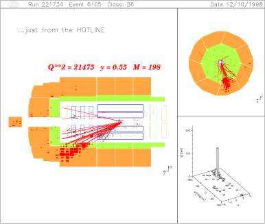
Figure 4: A jet in deep-inelastic scattering. Event recorded at the H1 experiment at HERA.

Figure 5: A jet pair in $\rm e^{+}e^{-}$ annihilation. Event recorded at the Opal experiment at LEP.

Figure 6: Jet pair at a hadron collider. Event recorded by the D0 experiment at Fermilab.

2.3 How to calculate jet cross sections

Clearly, we can observe the jets, but we still have to ask whether we can calculate anything about them. Here we can hope to benefit from the asymptotic freedom of QCD, but as we’ve seen, we have to be careful – the S-matrix cannot be treated by short-distance analysis alone. If so, how can we hope to compute cross sections?

We can get insight into the challenges involved, and their possible solutions, by recalling the related “infrared problem” of QED, and its “solution”. As is often the case, the problem is related to asking the wrong question, and the solution to identifying the right one.

In QED, typical exclusive cross sections have infrared divergent corrections in perturbation theory, which show up as logarithmic dependence on the (vanishing) mass of the photon. This happens as soon as we go to the order $\alpha_{\rm EM}\equiv e^{2}/4\pi$ correction of a Born cross section, say in electron-electron scattering at momentum transfer $Q$:

$$\sigma^{(1)}_{{\rm ee\rightarrow ee}}\left(Q,m_{e},\ {m_{\gamma}\rightarrow 0},\alpha_{\rm EM}\right)\sim\alpha_{\rm EM}\;\beta_{{\rm ee\rightarrow ee}}(Q/m_{e})\;{\ln{Q\over m_{\gamma}}}\,,$$ (10)

with $\beta_{{\rm ee\rightarrow ee}}(Q/m_{e})$ a function that is finite for vanishing photon mass, $m_{\gamma}$. Following the famous Bloch-Nordsieck analysis [13], however, we trace this divergence to asking an unphysical question, the probability for one or more charged particles to scatter, and in the process be accelerated, while emitting no radiation at all. In effect, we are computing the probability of something that never happens.

The classical theory demands radiation, and classical radiation requires an essentially unlimited number of very low-energy photons. This is Bohr’s correspondence principle between quantum and classical mechanics. Rather than count the number of photons (zero, one …), Bloch and Nordsieck [13] counseled that we introduce an energy resolution, $\epsilon Q$ with $\epsilon\ll 1$, and then sum over final states with arbitrary photon emission, as long as the total energy comes in below the energy resolution. Experimentally, this is not a choice, but a necessity, because our apparatus will always miss some photons if they are soft enough. At first, however, it sounds complicated. How can we sum over all soft photons? But this will not be necessary.

Following the Bloch-Nordsieck procedure, suddenly the full order $\alpha_{\rm EM}$ correction with an energy resolution becomes finite by itself, the log of $m_{\gamma}/Q$ being replaced by a log of $\epsilon$, as the result of a cancellation between the final states with and without an extra photon. As long as $\alpha_{\rm EM}\ln(1/\epsilon)\ll 1$ (which is almost inevitable), the correction is small,

$$\overline{\sigma}^{(1)}_{{\rm ee\rightarrow ee}+X(\epsilon)}\left(Q,m_{e},{\epsilon Q},\alpha_{\rm EM}\right)\sim\alpha_{\rm EM}\;\beta_{{\rm ee\rightarrow ee}}(Q/m_{e})\;{\ln{1\over\epsilon}}\,.$$ (11)

The magic (and beauty) of this is that we don’t have to sum over an infinite number of soft photons, even though this is the root cause of the problem!

Now let’s think about QED in the very high-energy limit. On a closer look, we find that the function $\beta_{{\rm ee\rightarrow ee}}(Q/m_{e})$ itself has a log of $Q/m_{e}$. Given that the dominant term depends only on the ratio, we can as well trade the high-energy limit for the double, photon-and-electron, zero mass limit. But in this case, our energy resolution is not enough to produce finite cross sections. If, however, we can solve this problem in QED, we may be able to solve it as well in high-energy QCD, where the high-energy limit also involves logarithmic enhancements in ratios of momenta to all particle masses.

We wish to look for quantities that are capable of measurement, have a single hard momentum scale, $Q$, and which nevertheless have no powers of $\ln(Q/m)$, only at worst $(m/Q)\ln(Q/m)$. Such quantities become functions of only that single hard scale, and are calculable as a power series in the coupling $\alpha_{s}(\mu)$, with $\mu=Q$, without introducing any large ratios when $Q\rightarrow\infty$ with fixed masses, or equivalently $m\rightarrow 0$ at fixed $Q$. These are quantities for which asymptotic freedom can be naturally applied, and are, in the terminology mentioned above, infrared safe.

We’ve already seen that an energy resolution alone is not enough for infrared safety. Progress can be made, however, by an analogy to the argument for an energy resolution based on the unobservability of arbitrarily soft photons. We can just as well say that two exactly collinear massless particles cannot be distinguished from a single massless particle of the same total momentum (and total quantum numbers), whether that momentum is soft or not. That is, if $p^{2}=0$ and $p^{\prime}{}^{2}=0$ and if $p^{\mu}$ and $p^{\prime}{}^{\mu}$ are collinear, then $(p+p^{\prime})^{2}=0$ as well. So whether the combination is a single particle or two particles is not easy to distinguish.

This approach works, and enables us to take the zero-mass limit for all particles in QED and QCD. Roughly speaking, any cross section with an energy and an angular resolution is infrared safe in $\rm e^{+}e^{-}$ annihilation [14]. If two particles are closer together in direction than some angle, $\delta$, then we treat them the same way as we do a single particle. We’ll also see that hadron-hadron cross sections of this sort, while not themselves infrared safe, contain an infrared safe factor that we can isolate.

The conditions for infrared safety may also be rephrased in a more general form as follows. Any cross section that sums over all states that (1) differ by the emission or aborption of soft particles, or (2) by the splitting or recombination of exactly collinear particles, is infrared safe [14, 15, 16, 17, 18, 19] (or contains an infrared safe factor.) It is worth noting that to prove infrared safety for jet cross sections requires an extension of the beautiful theorems that apply to fully inclusive transition probabilities [20]. This involves a careful reanalysis of perturbation theory, and is especially dependent on how the gauge invariance of the theory manifests itself [16].

The most direct application of infrared safety is to jet cross sections in $\rm e^{+}e^{-}$ annihilation, exactly of the type illustrated schematically by Fig. 3 and in experiment by Fig. 5. So long as the resolutions are large, we can represent the use of asymptotic freedom for jet cross sections by an appropriate choice of renormalization scale, taken here as the total energy $Q$,

$$\sigma\left(Q/\mu,\epsilon,\delta,\alpha_{s}(\mu)\right)=\sigma\left(1,\epsilon,\delta,\alpha_{s}(Q)\right)\,,$$ (12)

where $\epsilon$ and $\delta$ represent the energy and angular resolutions mentioned above, or more generally other parameters that define the cross section. Computed in this fashion, there is no need for a transverse momentum cutoff of the sort invoked in Ref. [11]. The infrared safety of the observable ensures that high-$p_{T}$ radiation is suppressed by factors of $\alpha_{s}(p_{T})$. Such radiation is present, of course, but it influences the infrared safe quantity through calculable corrections, just as the effects of soft gluons influence QED cross sections in a finite way at higher orders.

2.4 The field-theoretic content of infrared safety

Summarizing, we recount the “sorrows” of QCD perturbation theory, and how they can be overcome, at least in part. First, there is color confinement, which may be interpreted as the statement that matrix elements like

$$\int d^{4}x\,{\rm e}^{-ip\cdot x}\langle 0|\,T[q_{a}(x)\dots]\,|0\rangle\,,$$ (13)

in which we take the Fourier transform of a quark or other field with a nontrivial color representation has no $p^{2}=m^{2}$ pole in a Green function, with $T$ time-ordering. (This is confinement.) Second, poles at physical particle masses, such as $p^{2}=m_{\pi}^{2}$ for pions,

$$\int d^{4}x\,{\rm e}^{-ip\cdot x}\langle 0|\,T[\pi(x)\dots]\,|0\rangle\,,$$ (14)

are not accessible to perturbation theory.

Despite all this, we are able to use infrared safety and asymptotic freedom for such quantities as the total cross section for $\rm e^{+}e^{-}$ annihilation into hadrons. What are we really calculating? Totally inclusive examples like these are related by the optical theorem to forward-scattering amplitudes of the general form

$$\int d^{4}x\,{\rm e}^{-iq\cdot x}\langle 0|\,T[J(x)J(0)]\,|0\rangle\,,$$ (15)

involving color singlet currents, just as in Eq. (8). Deep-inelastic scattering involves hadronic matrix elements rather than the ground state [17, 18],

$$W_{\mu\nu} = 2\ {\rm Im}\,{i\over 8\pi}\int d^{4}x\,e^{-iq\cdot x}<N(p)|\;T[\;J_{\mu}(x)J_{\nu}(0)\;]\;|N(p)>$$ (16)

$$= -\left(g_{\mu\nu}-\frac{q_{\mu}q_{\nu}}{q^{2}}\right)\,F_{1}(x,Q^{2})$$

$$\hskip 28.45274pt+\left(p_{\mu}-q_{\mu}\frac{p\cdot q}{q^{2}}\right)\left(p_{\nu}-q_{\nu}\frac{p\cdot q}{q^{2}}\right)\,\frac{1}{p\cdot q}\,F_{2}(x,Q^{2})\,,$$

for electroweak currents, $J_{\mu}$, and nucleon states, $|N(p)\rangle$, with $x\equiv p\cdot q/Q^{2}$ and $q^{2}=-Q^{2}<0$. The $F_{i}(x,Q^{2})$ are the same structure functions as shown in Fig. 2. For such matrix elements, we will apply factorization properties, which will enable us to isolate the infrared safe factors referred to above.

Another class of color singlet matrix elements enables us to describe jet-related cross sections [21]. These look like

$$\lim_{R\to\infty}\,R^{2}\,\int dx_{0}\int d\hat{n}\,f(\hat{n})\,{\rm e}^{-iq\cdot y}\langle 0|\,J(0)T[\hat{n}_{i}T_{0i}(x_{0},R\hat{n})J(y)]\,|0\rangle\,,$$ (17)

with $T_{0i}$ the energy momentum tensor, and $\hat{n}$ a vector on the unit sphere. Such a matrix element represents the action of a calorimetric detector, which measures energy flow, and matrix elements such as these are what we really calculate when we compute jet cross sections. For a general cross section, we introduce a “weight”, given by function $f(\hat{n})$. As long as all the derivatives, $d^{r}f(\hat{n})/d\hat{n}^{r}$, of the weight are bounded, individual final states may have infrared divergences, but they cancel in the sum over collinear splitting/merging and soft parton emission, because these transitions respect energy flow [16]. We regularize the divergences dimensionally (typically) and calculate the long-distance enhancements in amplitudes, only to cancel them in infrared safe cross sections. It is this intermediate step that makes many calculations tough, and is part (not all) of why higher-order calculations are so difficult. It may be worth noting that one of the goals of a collider experiment is remarkably similar – to control late stage interactions of particles once they enter the detectors.

3 Extracting Infrared Safety: Factorization

Any cross section with one or two hadrons in the initial state has inescapable long-distance behavior, because a semi-inclusive sum over initial states is simply not a practical option. In effect, we can choose the energy of the nucleon(s) that initiate our scattering process, and sometimes their spin, but little else. By construction, then, cross sections at hadronic colliders are not infrared safe. The technqiue of factorization, however, enables us to isolate and extract infrared safe dependence in a large set of otherwise long-distance phenomena. Here we review the physical basis of factorization, and show how the factorization of a process also leads to useful information on its energy-dependence, including the evolution of the moments of parton distributions, as in Eq. (4) above.

3.1 Factorization

The general form of a factorized cross section (here multiplied by $Q^{2}$ to make it dimensionless), is [22, 23]

$$Q^{2}\sigma_{\rm phys}(Q,m)={\omega_{\rm SD}(Q/\mu,\alpha_{s}(\mu))}\,\otimes\,f_{\rm LD}(\mu,m)+{\cal O}\left({1/Q^{p}}\right)\,,$$ (18)

where as shown on the left, the “physical” cross section $\sigma$ depends generically on a hard scale $Q$ and on a wealth of soft scales, denoted collectively by $m$. The soft scales include in general the gluon mass, which is zero, as well as various quark masses, and the scale of the perturbative coupling, $\Lambda_{\rm QCD}$, encoded in the running coupling, Eq. (2).

On the right of Eq. (18), we give the schematic factorized form of $\sigma$, in which the $Q$-dependence and $m$-dependence are separated. There is a short-distance function $\omega_{\rm SD}$, which is infrared safe, and a long-distance function $f_{\rm LD}$, which for hadronic initial states is not calculable in perturbation theory. The short- and long-distance functions are linked by a convolution, denoted $\otimes$. For deep-inelastic or hadron-hadron scattering the convolution is in partonic momentum fractions, “$x$”, which is transformed into a simple product by the moments leading to Eq. (4) above.

Dimensional analysis requires that we introduce a new scale, $\mu$, the factorization scale, so that $\omega_{\rm SD}$ and $f_{\rm LD}$ can be nontrivial functions of $Q$ and $m$, respectively. In effect, the factorization scale marks the boundary between short-distance and long-distance dependence.

As indicated in Eq. (18), factorization is not normally an exact result, but it often holds up to corrections that behave as inverse powers of $Q$. For many important examples, such as unpolarized deep-inelastic scattering cross sections, corrections enter only as $1/Q^{2}$, and are negligible for many purposes once $Q$ reaches several GeV.

In the most familiar examples, including the structure functions $F_{1}$ and $F_{2}$ in (16), the $f_{\rm LD}$ are parton distributions, and we shall refer to them as such. The parton distributions themselves can be expressed in terms of expectation values [24] in hadronic states that fix light-cone components of the momenta of the partons in question. We take the light-cone components for any vector $v^{\mu}$ as $v^{\pm}=(1/\sqrt{2})(v^{0}\pm v^{3})$, with $v^{2}=2v^{+}v^{-}-v_{T}^{2}$. A vector whose only nonvanishing component is $v^{+}$ or $v^{-}$ is light-like, $v^{2}=0$.

For example, the (spin-averaged) distribution of quark $q$ in nucleon $N$ with momentum $p^{\mu}=p^{+}\delta_{\mu+}$, and spin $s$, is

$$f_{q/N}(x,\mu^{2}) = {1\over 2}\sum_{s}\int^{\infty}_{-\infty}{dy^{-}\over 2\pi}e^{-ixp^{+}y^{-}}\,<N(p,s)\mid\bar{q}(0^{+},y^{-},{\bf 0}_{\perp})$$ (19)

$$\hskip 42.67912pt\times\;\,{1\over 2}\gamma^{+}\;\Phi_{n}(y^{-},0)\;q(0)\mid N(p,s)>\,.$$

We can compare this form to the matrix element for currents, Eq. (16). In this case, the factorization scale, $\mu$, enters because we must renormalize the product of quark fields that are separated by a light-like distance $y^{-}$ in the minus direction. The operator $\Phi(y^{-},0)$ is a “gauge link”, between the two fields, whose purpose is to render the matrix element gauge invariant, and which is defined by

$$\Phi_{n}(y^{-},0)=P\exp\left[-ig\int_{0}^{y^{-}}dl\;n\cdot A(ln^{\mu})\right]\,,$$ (20)

with $n^{\mu}=\delta_{\mu-}$. Here the field $A^{\mu}=\sum_{a}A^{\mu}_{a}T_{a}$ is given as a matrix in terms of the relevant generators of SU(3), which for quarks are in fundamental ($3\times 3$) representation. The symbol $P$ denotes an ordering of these color matrices along the path between $l=0$ and $l=y^{-}$.

3.2 From factorization to evolution

If we can factorize a cross section as in Eq. (18), its $Q$-dependence is calculable. As such, we can compute it systematically in extensions of the standard model that include new heavy states, which modify the short-distance behavior of the theory. “New physics”, then, is embedded in a calculable fashion in $\omega_{\rm SD}$. While not calculable in perturbation theory, the functions $f_{\rm LD}$ are “universal”, portable from one factorizable process to another.

The key to the portability of parton distributions, is their “evolution”, which enables us to compute their dependence on the factorization scale [25]. Calculable evolution is not a separate assumption, but rather a direct consequence of the factorization in Eq. (18). We need only observe that the physical cross section cannot depend on the factorization scale,

$$0=\mu{d\over d\mu}\ln\sigma_{\rm phys}(Q,m)\,.$$ (21)

We can thus separate dependence on $Q$ and $m$ by requiring that the $\mu$-dependence of the short-distance function cancel that of the long-distance function,

$$\mu{d\ln\omega_{\rm SD}\over d\mu}=-P(\alpha_{s}(\mu))=-\mu{d\ln f_{\rm LD}\over d\mu}\,.$$ (22)

The “separation constant” $P(\alpha_{s})$ can depend only on those variables that the short- and long-distance functions hold in common: the coupling and the convolution variables. Eq. (22) is an evolution equation. We can solve it to relate parton distributions at one $\mu$ to another, and therefore, because we can always choose $\mu=Q$ in Eq. (18), we can relate the cross section at one $Q$ to that at another scale, up to corrections associated with the expansion of $\omega_{\rm SD}(Q/\mu,\alpha_{s}(\mu))$ in the strong coupling. Of course, this analysis requires that $\alpha_{s}$ remain small in the range over which we wish to evolve. Schematically, then, we can exhibit the cross section’s dependence on the momentum transfer as

$$\sigma_{\rm phys}(Q,m)=\omega_{\rm SD}(1,\alpha_{s}(Q))\,\otimes\,\exp\left\{-\;\int_{Q_{0}}^{Q}{d\mu^{\prime}\over\mu^{\prime}}P\left(\alpha_{s}(\mu^{\prime})\right)\right\}f_{\rm LD}(Q_{0},m)\,,$$

just as in Eq. (4) for the moments of structure functions.

3.3 The pattern of a factorized cross section

A large class of hadronic cross sections can be factorized, as long as they are defined in a manner consistent with the energy flow interpretation described in the previous section. This involves, in general, observing a jet-like structure in the final state and summing over soft radiation between the jets. The general structure of any such observable falls into a form that can be represented schematically as

$${d\sigma_{a+b\rightarrow{\rm jets\,\{i\}}}(Q)\over dQ}=f_{a^{\prime}/a}\otimes f_{b^{\prime}/b}\,\otimes{H^{a^{\prime}+b^{\prime}\rightarrow\{d_{i}\}}_{IK}}\times{S^{a^{\prime}+b^{\prime}\rightarrow\{d_{i}\}}_{KI}}\times{\prod_{{\rm jets}\,\{i\}}J_{d_{i}}}\,.$$

(24)

We can think of this expression as recounting a (quantum-mechanical) story: evolved incoming partons represented by $f_{a^{\prime}/a}$, $f_{b^{\prime}/b}$ collide and exchange momenta at short distances. A function $H_{IK}$ describes quantum corrections at that scale ($Q$), where $K$ and $I$ identify color exchange in the amplitudes and their complex conjugates, respectively. These indices are in a color tensor basis that reflects the numbers and color representations of all the “active” partons, $a^{\prime}$, $b^{\prime}$, and $\{d_{i}\}$ [26]. In general, the color exchange at short distances influences the development of the system at long distances, through a color-exchange-dependent soft function, $S_{KI}$ describing the production of soft particles. Finally, the production of energetic particles and jets is described by a set of functions $J_{d_{i}}$, each specifying the fragmentation of the parent parton $d_{i}$ of jet $i$. These fragmentation processess are mutually incoherent, with a universal evolution into the final states that is itself the result of this factorization.

Eq. (24) holds in general to all powers of the coupling, with power corrections in hard scales. The latter, however, can be quite complex, involving ratios of the maximum soft energy to jet energies: $E_{\rm soft}/E_{\rm jet}$, but also inverse powers of the energy of soft radiation. That is, we also anticipate “power corrrections” of the form $m/E_{\rm soft}$, with $m$ any of the long-distance mass scales in the theory [27]. On the perturbative level, the very presence of a factorization involving soft, jet and short-distance functions ensures more elaborate evolutions, involving double-logarithmic corrections [28].

It is worth noting that the original cosmic ray jets were not of this sort. Their properties are not computable in quite the same way, because for the most part they lack truly high-momentum transfer subprocesses, represented by $H_{KI}$ in Eq. (24). For recent applications of perturbative QCD to such “inclusive” proton-nucleus and nucleus-nucleus cross sections, see Ref. [29].

A generalization of Eq. (24) applies in hadronic scattering to high-transverse momentum ($p_{T}$) single-particle inclusive cross sections. In this case, the jet functions of Eq. (24) are replaced by fragmentation functions,

$$d\sigma_{A+B\to H+X}(p_{T}) = \sum_{c}d\bar{\sigma}_{A+B\to c+X}(p_{T}/z\mu)\otimes D_{H/c}(z,m_{c},\mu)$$ (25)

$$\hskip 56.9055pt+{\mathcal{O}}(m_{c}^{2}/p_{T}^{2})\,,$$

with a sum over fragmenting partons $c$. The cross section $d\bar{\sigma}$ includes parton distributions for the initial state. Here, following the formalism developed by Collins and Soper [24], the fragmentation function, $D_{H/c}$ can be defined as a vacuum expectation value similar to those above for the distributions, but now involving creation and annihilation operators for the observed hadron. For a gluon to fragment to hadron $H$, for example, the function is [24]

$$D_{H/g}(z,m_{c},\mu) = -~{}\frac{1}{16(2\pi)P^{+}}{\mathrm{T}r}_{\mathrm{c}olor}\int dy^{-}{\mathrm{e}}^{-i(P^{+}/z)y^{-}}$$ (26)

$$\times\langle 0|G^{+\lambda}(0)\,{[\Phi_{-}^{(adj)}(0)]^{\dagger}}\,a_{H}^{\dagger}(P^{+})\,a_{H}(P^{+})\,{\Phi_{-}^{(adj)}(y^{-})}\,G^{+}{}_{\lambda}(y^{-})|0\rangle\,,$$

with $G^{\mu}{}_{\nu}$ the gluon field strength and $a_{H}^{\dagger}$ the creation operator for hadron $H$. The relevant ordered exponential, or gauge link, for this process is

$$\Phi_{-}^{(adj)}(x^{-})=P\exp\left[-ig\int_{0}^{\infty}n\cdot A^{(adj)}\left((x^{-}+\lambda)n\right)\,\right]\,,$$ (27)

where $n^{\mu}$ is a lightlike vector in the opposite direction to the jet. For gluon fragmentation, the gauge field $A^{(adj)}_{\mu}$ is an $8\times 8$ matrix in the adjoint representations of SU(3) generators. Such a gauge link gives rise to a nice set of diagrammatic rules, in terms of “eikonal lines” in the $x^{-}$ direction $(n^{\mu}=\delta_{\mu-})$, with vertices $-ign^{\mu}\times(group\ factors)$ and (linear) propagators $i/(n\cdot k)$, illustrated in Fig. 7. To the jet, as it fragments, all that’s left of the rest of the world is a gluon source moving in the opposite direction, whose entire influence is summarized by the eikonal line. Similar considerations apply to the parton distributions, Eq. (19).

Figure 7: Graphical representation of the ordered exponential, Eq. (27).

3.4 The classical basis of factorization

Where do factorized cross sections like Eq. (24) come from? In the following we review an argument based on the classical Lorentz transformation properties of fields, and point out the subtleties of gauge fields in particular [30]. An argument based on a classical picture isn’t far-fetched, precisely because, as noted above, the correspondence principle is the key to the origin of infrared divergences. Any accelerated charge must produce classical radiation, and infinite numbers of soft gluons are required to make a classical field. Thus the classical field has a lot to tell us about the radiation of soft partons.

Having said this much, we consider the situation illustrated in Fig. 8, in which one “bound state”, approaches another (from the left in the figure) at a relativistic velocity $\beta\rightarrow 1$ in the $x_{3}$-direction, carrying with it various point charges, its “partons”. The coordinates of the bound state on the left are indicated by unprimed variables, those on the right by primed. We will refer to the former as the projectile, the latter as the target.

Suppose the partons of our projectile are sources for a massless scalar field, whose magnitude we denote by $\phi$. In their own rest frames, the sources produce a simple $1/|\vec{x}|$ potential. By definition, the magnitude of a scalar field at any point in space-time is independent of the coordinate system in which it is observed. We can thus start with an expression for our massless scalar field in the rest frame of the projectile, and simply reexpress it in terms of the coordinates of the target. To do so we use $x_{3}=\gamma(\beta ct^{\prime}-x^{\prime}_{3})\equiv\gamma\Delta^{\prime}$, where as usual $\gamma=(1-\beta^{2})^{-1/2}$. This gives

$${\phi(x)\ =\ {q\over\sqrt{x_{T}^{2}+x_{3}^{2}}}}\ =\ \phi^{\prime}(x^{\prime})\ =\ {q\over(x_{T}^{2}+{\gamma^{2}}\Delta^{\prime}{}^{2})^{1/2}}\,,$$ (28)

where $q$ is a charge and $x_{T}$ the distance of closest approach, which is transverse to the motion. Naturally, the field is maximized in the target coordinates at the time of closest approach, where $\Delta^{\prime}=0$, that is, at $t^{\prime}=\frac{1}{\beta c}x^{\prime}_{3}$. At this target time, the magnitude of the field is simply $q/x^{\prime}_{T}$. At all other values of the time $t^{\prime}$, however, the field of the oncoming projectile partons is proportional to an explicit factor of $1/\gamma$. In summary, the scalar field transforms “like a ruler”, that is, at any fixed $\Delta^{\prime}\neq 0$, the field decreases like $1/\gamma=\sqrt{1-\beta^{2}}$ as $\gamma\rightarrow\infty$. This is to say that for any fixed time in the target frame before closest approach, the field of the projectile decreases rapidly as the velocity of the projectile approaches the speed of light. This is just a consequence of length contraction in elementary special relativity. When an observer riding on the projectile (!) measures a distance $x_{3}$, then an observer sitting on the target measures a much larger distance.

                                                                            

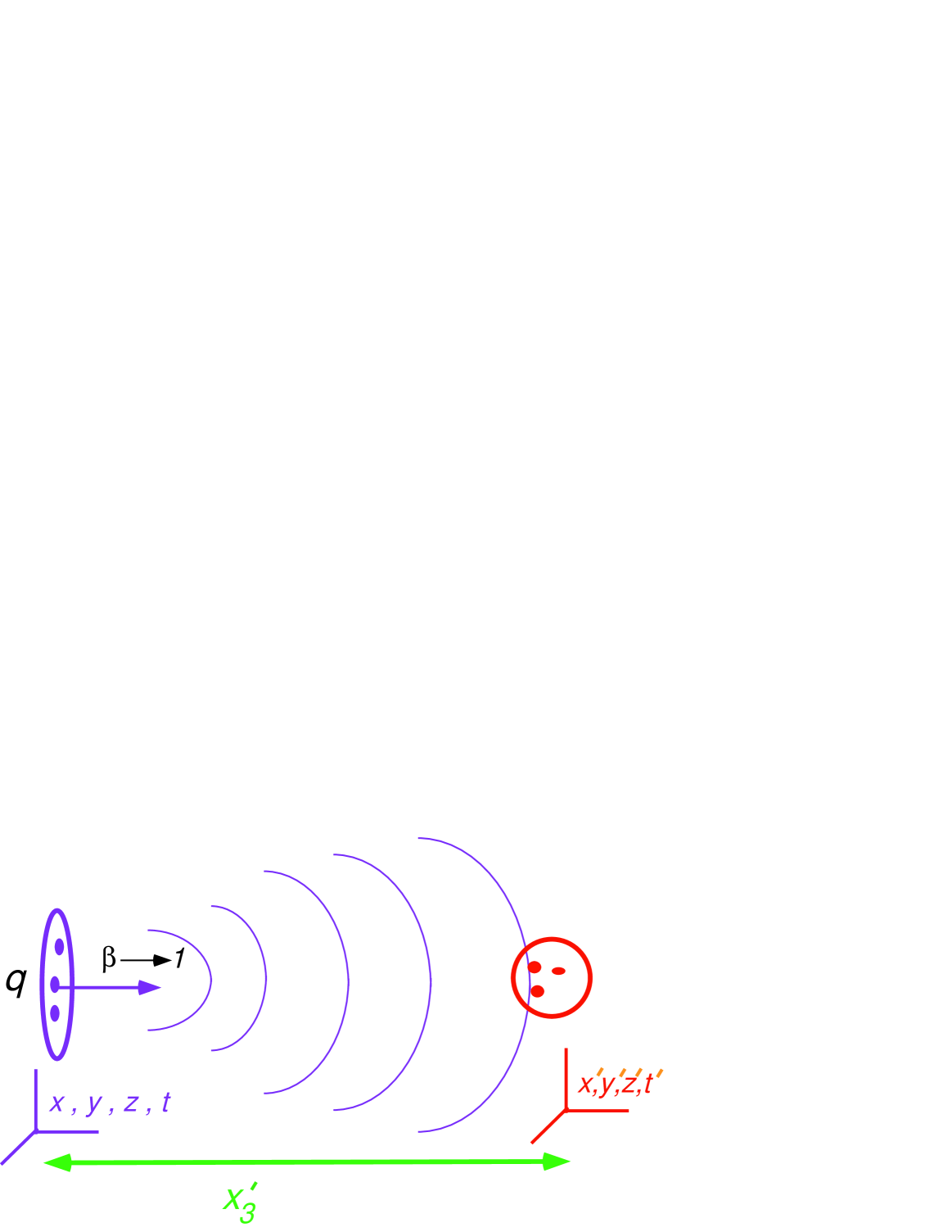
Figure 8: Schematic representation of the field of an oncoming particle.

Next, we suppose that the sources of the projectile couple to the electromagnetic field instead of a scalar field, producing in their own rest frames the same $1/|\vec{x}|$ potential, but now as the zeroth component of the vector $A^{\mu}(x)$. The following array compares gauge fields to scalar fields from this point of view. We compare, on the one hand, the $A^{0}$ component of the field in the projectile frame to the $A^{0}$ component in the target frame, found by Lorentz transformation, and on the other hand the longitudinal (third) component of the electric field in both frames,

$$\begin{array}[]{ccc}\underline{{\rm field}}&\underline{x\ {\rm frame}}&\underline{x^{\prime}\ {\rm frame}}\vspace{8mm}\\ {\rm scalar}&{q\over|\vec{x}|}&{q\over(x_{T}^{2}+{\gamma^{2}}\Delta^{2})^{1/2}\vspace{8mm}}\\ {\rm gauge}&A^{0}(x)={q\over|\vec{x}|}&A^{\prime}{}^{0}(x^{\prime})={q{\gamma}\beta\over(x_{T}^{2}+{\gamma^{2}}\Delta^{2})^{1/2}\vspace{8mm}}\\ {\rm field\ strength}&\hskip 28.45274ptE_{3}(x)={-q\over|\vec{x}|^{2}}&E_{3}^{\prime}(x^{\prime})={-q{\gamma}{\Delta}\over(x_{T}^{2}+{\gamma^{2}}\Delta^{2})^{3/2}}\,.\\ \\ \end{array}$$ (34)

We can ask the same question of the electromagnetic potential and field strength that we posed for the scalar field: at a fixed target time before the point of closest approach, how does the field observed at the target depend on the velocity of the projectile? The answers for the gauge field and the field strength are strikingly different. The gauge potential is actually independent of $\gamma$ as $\beta\rightarrow 1$ for any fixed $\Delta^{\prime}\neq 0$! The vector potential (at least its time component) is not contracted at all. On the other hand, the field strength, as represented by $E_{3}$, decreases as $1/\gamma^{2}$, which is a much more rapid decrease than even the scalar field.

These two behaviors are, of course, consistent, and are reconciled by the realization that the vector field of a relativistic charge approaches a total derivative in the target (primed) frame as $\beta\rightarrow 1$,

$$A^{\prime}\,{}^{\mu}(x^{\prime})=q\frac{\partial}{\partial x^{\prime}_{\mu}}\ \ln\left(\beta ct^{\prime}\,-\,x^{\prime}_{3}\right)+{\cal O}(1-\beta)\,.$$ (35)

The bulk of this $A^{\mu}$ is actually an unphysical polarization, and can be removed by a gauge transformation. In contrast, the physical “force” field $\vec{\bf E}$ of the projectile does not overlap the target until the moment of closest approach. “Advanced” effects in the electric field are corrections to the total derivative in Eq. (35), and hence are of the size

$$1-\beta\ \sim\ \frac{1}{2}\;\left[\sqrt{1-\beta^{2}}\right]^{2}\ \sim\ \frac{m^{2}}{2\omega^{\prime}{}^{2}}\,,$$ (36)

where $m$ is the mass of the projectile, and $\omega^{\prime}$ its energy in the target frame. This is a power-suppressed behavior, and a typical initial-state correction to factorization.

Factorization expresses this contraction effect. As the oncoming projectile approaches the speed of light, the appearance of its field is essentially instantaneous at the time of closest approach. The projectile then cannot affect the internal structure of the target, or vice-versa, and the target’s internal structure is thus effectively universal among all projectiles, so long as the latter are sufficiently relativistic. The initial state structure of the target and projectile can then both be summarized by multiplicative factors, and these are the parton distributions of Eq. (24).

This argument, of course, applies only to initial-state interactions, signals exchanged before the hard interaction. For final-state processes to respect factorizations like Eq. (24), it is also necessary that we define the observable in a manner consistent with infrared safety. In addition, for factorization to hold, we must require that there be a hard scattering. Otherwise there is no well-defined time at which the scattering occurs, and indeed no sharp distinction between the initial state and the final state. If there is a well-defined hard scattering, however, low-momentum transfers after that scattering are too late to affect the large momentum transfer process(es), such as the creation of jets or of heavy particles. Similarly, the fragmentation of partons into jets of hadrons is too late to know details of the hard scattering, leading to the factorization of fragmentation functions.

3.5 Factorization in perturbation theory

Perturbative arguments for factorization in QCD [22, 23] are, unfortunately, much more complex than the simple classical pictures above. Nevertheless, the physical observations we have just made have a direct correlation in perturbation theory, which is worth pointing out. We consider a soft gluon, of momentum $k$ emitted by a fast quark, whose momentum $p^{\mu}$ is on-shell $(p^{2}=m^{2})$ just after this interaction. In perturbation theory, this will be associated with a factor like

$$\bar{u}(p)\;(-ig\,\gamma^{\mu}\,)\;\frac{\hbox to0.0pt{\it p\hss}{/}+\hbox to0.0pt{\it k\hss}{/}\;+\;m}{(p+k)^{2}\ -\ m^{2}}\ =\ \bar{u}(p)\;(-ig\,)\;\frac{p^{\mu}}{p\cdot k}\ +\ (IR\ finite)\,,$$

where in the second form we have used the Dirac equation, and have suppressed terms proportional to $k$, which are infrared finite, as well as color factors. In an arbitrary perturbative diagram, the vector $p^{\mu}$ on the right-hand side will be contracted with the propagator of the soft gluon that carries momentum $k$. Now suppose we were to choose a gauge for which $p\cdot A=0$, in which case the gluon propagator is given (with $p^{2}=0$) by

$$G^{\nu\mu}(k)=-\,\frac{i}{k^{2}}\;\left(g^{\nu\mu}\ -\frac{p^{\nu}\,k^{\mu}\,+\,k^{\nu}\,p^{\mu}}{p\cdot k}\,\right)\,.$$ (38)

In this gauge, the soft gluons decouple from the quark. This argument can easily be generalized beyond lowest order, and applies to the entire set of collinear partons, whether quark, antiquark or gluon, in that jet. No gauge choice like this, of course, can decouple soft gluons from more than one jet at a time. But the existence of such a gauge for each jet implies that soft gluon couplings cannot resolve more than the direction and overall color of a jet [23, 31]. This is the origin of the “universality” of soft gluon interactions, and their summary in terms of eikonal lines like those of Eq. (27) and Fig. 7, which play a central role in factorization for perturbative QCD.

4 Conclusion

We have summarized a few of the major results of perturbative QCD, which underly the basic applications of the theory to hadron-hadron and hadron-lepton collisions at large momentum transfer. We have presented justifications wherever they can be found, in both classical and quantum intuition.

The coming decade will see unprecedented applications of the ideas and methods of perturbative QCD at the Large Hadron Collider, in proton-proton, proton-nucleus and nucleus-nucleus experiments. Whether as a pesky background to new physics searches, or as a subject of interest in its own right, QCD, with its self-generated scales and evolving degrees of freedom, will remain a benchmark for our understanding of physics at its most challenging.

References

- [1] H. Fritzsch, M. Gell-Mann and H. Leutwyler Phys. Lett. B47, 365 (1973).
- [2] C.N. Yang and R.L. Mills, Phys. Rev. 96, 191 (1954).
- [3] S. Weinberg, Phys. Rev. Lett. 31, 494 (1973).
-
[4]
D.J. Gross and F. Wilczek, Phys. Rev. D8, 3633 (1973);
H.D. Politzer, Phys. Rept. 14, 129 (1974). - [5] J.D. Bjorken, Phys. Rev. 179, 1547 (1969).
-
[6]
R.A. Brandt and G. Preparata, Nucl. Phys. B27, 541
(1971);
Y. Frishman, Phys. Rev. Lett. 25, 966 (1970). - [7] N. Christ B. Hasslacher and A.H. Mueller, Phys. Rev. D6, 3543 (1972).
- [8] R.P. Feynman, Phys. Rev. Lett. 23, 1415 (1969).
-
[9]
S. Moch, J.A.M. Vermaseren and A. Vogt,
Nucl. Phys. B688, 101 (2004)
hep-ph/0403192;
A. Vogt, S. Moch and J.A.M. Vermaseren, Nucl. Phys. B691, 129 (2004) hep-ph/0404111. - [10] B. Edwards et al., Phil. Mag. 3, 237 (1957). The earliest mention of “jets” (still in quotations) that I have found is in R.R. Daniel et al., Phil. Mag. 43, 753 (1952).
- [11] S.D. Drell, D.J. Levy and T.M. Yan, Phys. Rev. D1, 1617 (1969).
- [12] G. Hanson et al., Phys. Rev. Lett. 35, 1609 (1975).
-
[13]
F. Bloch and A. Nordsieck, Phys. Rev. 52, 54
(1937);
D.R. Yennie, S.C. Frautschi and H. Suura, Annals Phys. 13, 379 (1961). - [14] G. Sterman and S. Weinberg, Phys. Rev. Lett. 39, 1436 (1977).
-
[15]
H.D. Politzer, Phys. Lett. B70, 430 (1977);
A. De Rujula, John R. Ellis, E.G. Floratos and M.K. Gaillard, Nucl. Phys. B138, 387 (1978). - [16] G. Sterman, Phys. Rev. D17, 2773; 2789 (1978); Phys. Rev. D 19, 3135 (1979).
- [17] G. Sterman, An Introduction to quantum field theory, Cambridge, UK: Univ. Pr. (1993) 572 p.
- [18] R. Brock et al. [CTEQ Collaboration], Rev. Mod. Phys. 67 (1995) 157.
- [19] M. Dasgupta and G. P. Salam, J. Phys. G 30, R143 (2004) [arXiv:hep-ph/0312283].
-
[20]
T. Kinoshita, J. Math. Phys. 3, 650 (1962);
T.D. Lee and M. Nauenberg, Phys. Rev. 133, B1549 (1964). -
[21]
N. A. Sveshnikov and F. V. Tkachov,
Phys. Lett. B 382, 403 (1996)
[arXiv:hep-ph/9512370];
G. P. Korchemsky, G. Oderda and G. Sterman, in DIS 97, AIP Conf. Proc. No. 407, ed. J. Repond and D. Krakauer, (American Institute of Physics, Woodbury, NY, 1997), p. 988. arXiv:hep-ph/9708346;
C. W. Bauer, S. P. Fleming, C. Lee and G. Sterman, arXiv:0801.4569 [hep-ph];
D. M. Hofman and J. Maldacena, arXiv:0803.1467 [hep-th]. -
[22]
G.T. Bodwin, Phys. Rev. D31, 2616 (1985),
Erratum ibid. D34, 3932 (1986);
J.C. Collins, D.E. Soper and G. Sterman, Nucl. Phys. B261, 104 (1985); ibid. B308, 833 (1988). - [23] J.C. Collins, D.E. Soper and G. Sterman, in Perturbative quantum chromodynamics, ed. A.H. Mueller (World Scientific, Singapore, 1989), p. 1, hep-ph/0409313.
- [24] J.C. Collins and D.E. Soper, Nucl. Phys. B194, 445 (1982).
-
[25]
G. Altarelli and G. Parisi, Nucl. Phys. B126, 298 (1977);
V.N. Gribov and L.N. Lipatov, Sov. J. Nucl. Phys. 15, 438, 675 (1972);
Yu.L. Dokshitzer, Sov. Phys. JETP 46, 641 (1977). - [26] N. Kidonakis, G. Oderda and G. Sterman, Nucl. Phys. B 531, 365 (1998) [arXiv:hep-ph/9803241].
-
[27]
M. Dasgupta and Y. Delenda,
JHEP 0711, 013 (2007)
[arXiv:0709.3309 [hep-ph]];
M. Dasgupta, L. Magnea and G. P. Salam, JHEP 0802, 055 (2008) [arXiv:0712.3014 [hep-ph]]. - [28] H. Contopanagos, E. Laenen and G. Sterman, Nucl. Phys. B 484, 303 (1997) [arXiv:hep-ph/9604313].
- [29] N. Armesto et al., J. Phys. G 35, 054001 (2008) [arXiv:0711.0974 [hep-ph]].
- [30] R. Basu, A.J. Ramalho and G. Sterman, Nucl. Phys. B 244, 221 (1984).
- [31] R. Tucci, Phys. Rev. D 32, 945 (1985) [Erratum-ibid. D 34, 1235 (1986)].