Comments on the Dynamics of the Pais–Uhlenbeck Oscillator

Comments on the Dynamics
of the Pais–Uhlenbeck Oscillator

Andrei V. SMILGA 

A.V. Smilga

SUBATECH, Université de Nantes, 4 rue Alfred Kastler, BP 20722, Nantes 44307, France smilga@subatech.in2p3.fr

Received November 24, 2008, in final form February 05, 2009; Published online February 12, 2009

We discuss the quantum dynamics of the PU oscillator, i.e. the system with the Lagrangian

$$L=\frac{1}{2}\left[\ddot{q}^{2}-(\Omega_{1}^{2}+\Omega_{2}^{2})\dot{q}^{2}+\Omega_{1}^{2}\Omega_{2}^{2}q\right]\ \ ({\rm+\ nonlinear\ terms}).$$ (1)

When $\Omega_{1}\neq\Omega_{2}$, the free PU oscillator has a pure point spectrum that is dense everywhere. When $\Omega_{1}=\Omega_{2}$, the spectrum is continuous, $E\in\{-\infty,\infty\}$. The spectrum is not bounded from below, but that is not disastrous as the Hamiltonian is Hermitian and the evolution operator is unitary. Generically, the inclusion of interaction terms breaks unitarity, but in some special cases unitarity is preserved. We discuss also the nonstandard realization of the PU oscillator suggested by Bender and Mannheim, where the spectrum of the free Hamiltonian is positive definite, but wave functions grow exponentially for large real values of canonical coordinates. The free nonstandard PU oscillator is unitary at $\Omega_{1}\neq\Omega_{2}$, but unitarity is broken in the equal frequencies limit.

higher derivatives; ghosts; unitarity

70H50; 70H14

1 Motivation

Mechanical and field-theory systems involving higher derivatives in the Lagrangian attracted (or, better to say, reattracted) recently some attention. In [2, 3] we put forward arguments that the Theory of Everything may represent a variant of supersymmetric higher-derivative theory living in flat higher-dimensional space. Our Universe is associated then with a 3-brane classical solution in this theory (a kind of soap bubble embedded in the flat higher-dimensional bulk), while gravity has the status of effective theory in the brane world-volume.

The first paper where such theories were considered dates back to 1950 [4]. It was shown there that higher-derivative theories are in many cases ghost-ridden, which may break unitarity and render theory meaningless. Recently, it was understood, however, that there are higher-derivative systems where the ghosts are “benign” such that unitarity is preserved. An example of nontrivial supersymmetric higher-derivative system of such benign variety was constructed and studied in [5].

In this note, we concentrate on the dynamics of the system (1) (it is the simplest example of higher-derivative mechanical systems introduced and studied first in the paper [4], which is known by the name Pais–Uhlenbeck oscillator). Recently, the interest to this problem has been revived [3, 6, 7, 8, 9, 10]. In spite of that many salient features of the PU oscillator dynamics were revealed in previous studies, a certain confusion persists now in the literature. This especially concerns the interpretation of the results obtained. Thus, we found it useful to write a kind of mini-review including all relevant previous results with inaccuracies corrected, as well as some new remarks. There are basically three new observations:

• The statement of [6] that the Hamiltonian of the oscillator in the equal frequency limit represents a set of Jordan blocks of infinite dimension is compatible with the statement that the spectrum of such system is continuous if the limit $\Omega_{1}\to\Omega_{2}$ is defined in a natural way [4, 7]. We note that the wave functions of continuous spectrum can be represented as superpositions of non-stationary solutions to the Schrödinger equation (non-stationary solutions are characteristic for Jordan block Hamiltonians.)

• In contrast to what we suggested earlier [6], the spectrum stays unbounded from below also when nonlinear terms in equation (1) are included. In most cases, the latter bring about the quantum collapse phenomenon and breaking of unitarity. Unitarity survives, however, when interaction has a certain special form.

• In contrast to what was written in [10], the free equal-frequency PU oscillator in the nonstandard realization is not unitary in the usual sense of this word.

2 Hamiltonian and its spectrum

The canonical Hamiltonian corresponding to the Lagrangian (1) can be obtained using Ostrogradsky’s method [11]. Due to the presence of extra derivatives, the phase space involves besides $(q,p_{q})$ an extra canonical coordinate

$$x=\dot{q}$$

and the corresponding canonical momentum $p_{x}$. The canonical Hamiltonian is

$$H=p_{q}x+\frac{p_{x}^{2}}{2}+\frac{\big{(}\Omega_{1}^{2}+\Omega_{2}^{2}\big{)}x^{2}}{2}-\frac{\Omega_{1}^{2}\Omega_{2}^{2}q^{2}}{2}.$$ (2)

Indeed, if writing the canonical Hamilton equations of motion and excluding $p_{q}$, $x$, $p_{x}$, we arrive at the equation

$$q^{(4)}+\big{(}\Omega_{1}^{2}+\Omega_{2}^{2}\big{)}\ddot{q}+\Omega_{1}^{2}\Omega_{2}^{2}q=0,$$

which can on the other hand be directly derived from the Lagrangian (1).

Consider first the case of inequal frequencies and assume for definiteness $\Omega_{1}>\Omega_{2}$. The Hamiltonian (2) can then be brought into diagonal form by the following canonical transformation

$$q=\frac{1}{\Omega}_{1}\frac{\Omega_{1}X_{2}-P_{1}}{\sqrt{\Omega_{1}^{2}-\Omega_{2}^{2}}},\qquad x=\frac{\Omega_{1}X_{1}-P_{2}}{\sqrt{\Omega_{1}^{2}-\Omega_{2}^{2}}},$$

$$p_{x}=\frac{\Omega_{1}P_{1}-\Omega_{2}^{2}X_{2}}{\sqrt{\Omega_{1}^{2}-\Omega_{2}^{2}}},\qquad p_{q}=\Omega_{1}\frac{\Omega_{1}P_{2}-\Omega_{2}^{2}X_{1}}{\sqrt{\Omega_{1}^{2}-\Omega_{2}^{2}}}.$$ (3)

The inverse of it is

$$X_{1}=\frac{1}{\Omega}_{1}\frac{p_{q}+\Omega_{1}^{2}x}{\sqrt{\Omega_{1}^{2}-\Omega_{2}^{2}}},\qquad X_{2}=\frac{p_{x}+\Omega_{1}^{2}q}{\sqrt{\Omega_{1}^{2}-\Omega_{2}^{2}}},$$

$$P_{1}=\Omega_{1}\frac{p_{x}+\Omega_{2}^{2}q}{\sqrt{\Omega_{1}^{2}-\Omega_{2}^{2}}},\qquad P_{2}=\frac{p_{q}+\Omega_{2}^{2}x}{\sqrt{\Omega_{1}^{2}-\Omega_{2}^{2}}}.$$ (4)

We obtain

$$H=\frac{P_{1}^{2}+\Omega_{1}^{2}X_{1}^{2}}{2}-\frac{P_{2}^{2}+\Omega_{2}^{2}X_{2}^{2}}{2}.$$ (5)

The spectrum of this Hamiltonian is

$$E_{nm}=\left(n+\frac{1}{2}\right)\Omega_{1}-\left(m+\frac{1}{2}\right)\Omega_{2},\qquad n,m=0,1,2,\ldots.$$ (6)

The eigenfunctions of the original Hamiltonian (2) are [6]

$$\Psi_{nm}(q,x)\ =\ C_{nm}e^{-i\Omega_{1}\Omega_{2}qx}\exp\left\{-\frac{\Delta}{2}\left(x^{2}+\Omega_{1}\Omega_{2}q^{2}\right)\right\}\phi_{nm}(q,x),$$ (7)

where $\Delta=\Omega_{1}-\Omega_{2}$ and

$$\phi_{nm}(q,x)=\sum_{k=0}^{m}\left(\frac{i\Delta}{4\sqrt{\Omega_{1}\Omega_{2}}}\right)^{k}\frac{m!(n-m)!}{(m-k)!k!(n-m+k)!}H^{+}_{n-m+k}H^{-}_{k},\qquad m\leq n,$$

$$\phi_{nm}(q,x)=\sum_{k=0}^{n}\left(\frac{i\Delta}{4\sqrt{\Omega_{1}\Omega_{2}}}\right)^{k}\frac{n!(m-n)!}{(n-k)!k!(m-n+k)!}H^{+}_{k}H^{-}_{m-n+k},\qquad m>n.$$ (8)

Here $H^{\pm}_{l}$ are the Hermite polynomials of the following arguments,

$$H_{l}^{+}\equiv\ H_{l}[i\sqrt{\Omega_{1}}(\Omega_{2}q-ix)],\qquad H_{l}^{-}\equiv\ H_{l}[\sqrt{\Omega_{2}}(\Omega_{1}q+ix)]$$

[$H_{0}(z)\equiv 1,H_{1}(z)\equiv 2z,H_{2}(z)\equiv 4z^{2}-2,\ldots$], and $C_{mn}$ are the irrelevant for our purposes normalization factors.

The wave functions (7) are normalized implying that the spectrum is pure point. However, for generic incommensurable frequencies, the spectrum is dense everywhere: however small the interval $\{E,E+dE\}$ is, it contains an infinite number of eigenvalues, and this is true for any $E$. Obviously, this unusual property is related to the fact that the spectrum has no bottom. We want to emphasize, however, that, though this quantum system is unusual, it is not sick: the Hamiltonian (5) is Hermitian and the corresponding evolution operator is unitary.

In the limit $\Omega_{1}\to\Omega_{2}$, the transformation (3) becomes singular. To understand what happens in this limit, it is best to look directly at the spectrum (6) and the wave functions (7), (8).

If setting formally $\Omega_{1}=\Omega_{2}$ in equation (6), we obtain

$$E_{nm}=\Omega(n-m)$$ (9)

meaning the infinite degeneracy of the spectrum at each level. The wave functions are reduced to

$$\Psi_{nm}(q,x)\ \propto\ \left[\begin{array}[]{c}e^{-i\Omega^{2}qx}H^{+}_{n-m},\qquad m\leq n,\vspace{1mm}\\ e^{-i\Omega^{2}qx}H^{-}_{m-n},\qquad m>n.\end{array}\right.$$ (12)

We see that, at each level with a given $n-m$, an infinite dimensional Jordan block appears [6].

3 Jordan blocks and continuous spectrum. Unitarity

The presence of Jordan blocks in the Hamiltonian implies usually the loss of unitarity. Indeed, consider the matrix Hamiltonian

$$H=\left(\begin{array}[]{cc}1&1\\ 0&1\end{array}\right)$$ (15)

(it has only one eigenvector $\psi=\left(\begin{array}[]{c}1\\ 0\end{array}\right)$ with eigenvalue 1). It is straightforward to see that the time-dependent Schrödinger equation

$$i\frac{d\psi}{dt}=H\psi$$ (16)

has the following general solution,

$$\psi(t)=a\left(\begin{array}[]{c}1\\ 0\end{array}\right)e^{-it}+b\left(\begin{array}[]{c}-it\\ 1\end{array}\right)e^{-it}.$$ (21)

When $b\neq 0$, the norm of $\psi(t)$ grows with time. The latter statement applies to the natural norm $\|\psi\|=\psi^{\dagger}\psi$ and also to any other positive definite norm $\sim\psi^{\dagger}M\psi$. If the norm is not positive definite, it is not true, as is clearly seen when choosing

$$M=\left(\begin{array}[]{cc}0&0\\ 0&1\end{array}\right).$$

Such a norm is degenerate, however. It projects the full 2-dimensional Hilbert space where the Hamiltonian (15) is defined to a one-dimensional subspace $\psi=\left(\begin{array}[]{c}0\\ c\end{array}\right)$. The dynamics in this subspace is unitary, the dynamics in full Hilbert space is not.

This reasoning applies to any Jordan block of finite dimension and to any Hamiltonian including such. However, in our case, the dimensions of the Jordan blocks are infinite. A remarkable fact is that in this case unitarity is not necessarily broken. In particular, a unitary evolution operator can well be defined for the free PU oscillator at equal frequencies. The novel feature compared to the inequal frequencies case is the appearance of continuous spectrum [4, 7].

Strong indications that the spectrum is continuous follow already from inspecting the spectrum (6), the wave functions (7), and their fate in the limit $\Omega_{1}\to\Omega_{2}$.

• One can notice first of all that the discrete spectrum (9) is only obtained from (6) if setting $\Omega_{1}=\Omega_{2}$ while keeping $n$, $m$ finite. It is possible to take the limit in such a way (this implies a kind of ultraviolet regularization), but a more natural approach is to allow $n$, $m$ to be arbitrary large. When $\Delta=\Omega_{1}-\Omega_{2}$ is sent to zero and $n,m$ are sent to infinity such that $n-m$ is kept fixed and $n\Delta$ is kept finite, the energy (6) can acquire an arbitrary value and not only the discrete values (9).

• In the limit $\Delta\to 0$, the wave functions (7) are no longer normalizable, and this suggests that the spectrum is continuous.

Let us now prove the continuity of the spectrum by constructing explicitly the wave functions of arbitrary energy $E$. At the first step, let us get rid of the terms $\propto x^{2}$ and $\propto q^{2}$ in the Hamiltonian by representing an eigenfunction of (2) as $\Psi(q,x)=e^{-i\Omega^{2}xq}\phi(q,x)$. The operator acting on $\phi(q,x)$ is

$$\tilde{H}=\frac{1}{2}p_{x}^{2}+xp_{q}-\Omega^{2}qp_{x}.$$ (22)

It is convenient then to perform the canonical transformation [4, 7]

$$p_{x}\to p_{x},\qquad p_{q}\to\Omega p_{q},\qquad x\to x+\frac{1}{4\Omega}p_{q},\qquad q\to\frac{1}{\Omega}q+\frac{1}{4\Omega^{2}}p_{x}.$$ (23)

giving the new Hamiltonian

$$H^{\prime}=\frac{p_{x}^{2}+p_{q}^{2}}{4}+\Omega(xp_{q}-qp_{x}).$$ (24)

The transformation (23) is the superposition of the scale transformation $q\to q/\Omega$, $p_{q}\to\Omega p_{q}$ and the unitary transformation $O\to e^{R}Oe^{-R}$ with $R=ip_{x}p_{q}/(4\Omega)$. The eigenfunctions of the Hamiltonian (22) is obtained from the eigenfunctions of the Hamiltonian (24) as

$$\phi(q,x)=\exp\left\{\frac{i}{4\Omega^{2}}\frac{\partial^{2}}{\partial x\partial q}\right\}\phi^{\prime}(\Omega q,x).$$

The eigenfunctions of $H^{\prime}$ are known,

$$\phi^{\prime}_{lk}(q^{\prime},x;t)\propto J_{l}(kr)e^{-il\theta}\,e^{-it(l\Omega+k^{2}/4)},$$

where $(r,\theta)$ are the polar coordinates in the plane $(q^{\prime},x)$ and $l=0,\pm 1,\pm 2,\ldots$ are the eigenvalues of the angular momentum operator ${L}=xp^{\prime}_{q}-q^{\prime}p_{x}$. We obtain

$$\phi_{lk}(q,x;t)\ \propto\ \exp\left\{\frac{i}{4\Omega^{2}}\frac{\partial^{2}}{\partial x\partial q}\right\}\left[J_{l}\left(k\sqrt{x^{2}+\Omega^{2}q^{2}}\right)\left(\frac{\Omega q-ix}{\Omega q+ix}\right)^{l/2}\right]e^{-it(l\Omega+k^{2}/4)}.$$

Introducing

$$z=\sqrt{\Omega}(x+i\Omega q),\qquad w=i\bar{z}=\sqrt{\Omega}(ix+\Omega q),$$

expanding the Bessel function and using the identity

$$\exp\left\{-\frac{1}{4}\frac{\partial^{2}}{\partial z^{2}}\right\}z^{n}=2^{-n}H_{n}(z),$$

we finally derive

$$\Psi_{lk}\ \propto\ e^{-it(l\Omega+k^{2}/4)}e^{-i\Omega^{2}qx}\sum_{m=0}^{\infty}\left(\frac{ik^{2}}{\Omega}\right)^{m}\frac{H_{l+m}(z)H_{m}(w)}{4^{2m+l}m!(l+m)!}.$$ (25)

The structure of this expression is similar to that in equations (7), (8), but the meaning is different: the expansion goes now in the spectral parameter $k^{2}/\Omega$ rather than in the parameter of the Hamiltonian $\Delta/\sqrt{\Omega_{1}\Omega_{2}}$ as in equation (8). In addition, equation (25) represents an infinite series rather than a finite sum. We can note that each level in the spectrum is infinitely degenerate. The eigenfuctions $\Psi_{lk}$, $\Psi_{l-1,\sqrt{k^{2}+4\Omega}}$, etc. have the same energy. This is not a Jordan degeneracy discussed above: the basis (25) diagonalizes the Hamiltonian, and the functions $\Psi_{lk}$ with different $l$ are distinguished by the eigenvalue of the “angular momentum” operator,

$$L=\frac{xp_{q}}{2\Omega}-\frac{\Omega}{2}qp_{x}+\frac{1}{4\Omega}\left(p_{x}^{2}-\frac{p_{q}^{2}}{\Omega^{2}}\right)+\frac{3\Omega x^{2}}{4}-\frac{3\Omega^{3}q^{2}}{4}$$

(we have rotated the operator ${L}=xp^{\prime}_{q}-q^{\prime}p_{x}$ back to original variables), that commutes with the Hamiltonian (2).

We have made two seemingly conflicting statements: $(i)$ the spectrum of the Hamiltonian involves a set of infinite-dimensional Jordan blocks and $(ii)$ the spectrum is continuous. How to reconcile them? To understand it better, consider the trivial free Hamiltonian

$$H=-\frac{1}{2}\frac{\partial^{2}}{\partial x^{2}}$$

with the eigenfunctions

$$\Psi(x;t)=\exp\left\{ikx-\frac{ik^{2}}{2}t\right\}.$$ (26)

Note now that not only (26), but also every term of its expansion in $k$,

$$k^{0}:\ \ \Psi_{0}(x;t)=1,$$

$$k^{1}:\ \ \Psi_{1}(x;t)=x,$$

$$k^{2}:\ \ \Psi_{2}(x;t)=t-ix^{2},$$

$$k^{3}:\ \ \Psi_{3}(x;t)=xt-\frac{ix^{3}}{3},$$

$$k^{4}:\ \ \Psi_{4}(x;t)=t^{2}-2itx^{2}-\frac{x^{4}}{3},$$ (27)

etc., satisfy the time-dependent Schrödinger equation (16). The functions (27) represent polynomials in $x$ and, what is especially noteworthy, in $t$, much similar to non-stationary solutions (21) characteristic to Jordan block Hamiltonians.

On the other hand, the functions (27) grow at large $x$, are not normalizable, and do not form a basis of a reasonable Hilbert space. The only way to define the latter is to sum over all $\Psi_{n}(x;t)$ with a proper weight and go back to the standard continuous spectrum wave functions (26), which can be dealt with by introducing a box of finite length $L$ (where the definition of Hilbert space presents no problem) and sending then $L$ to infinity.

By the same token, individual terms of the expansion of (25) in $k$ represent nonstationary solutions of the Schrödinger equation with the Hamiltonian (2). For $l=0$, these solutions are

$$k^{0}:\ \ e^{-i\Omega^{2}qx},$$

$$k^{2}:\ \ \big{[}t-i\big{(}x^{2}+\Omega^{2}q^{2}\big{)}\big{]}e^{-i\Omega^{2}qx},$$

$$k^{4}:\ \ \left[t^{2}-2it(x^{2}+\Omega^{2}q^{2})-\frac{(\Omega^{2}q^{2}+x^{2})^{2}}{2}-iqx+\frac{1}{8\Omega^{2}}\right]e^{-i\Omega^{2}qx},$$ (28)

etc. The first function in (28) coincides with the wave function (12) with $n-m=0$. The higher functions may be interpreted as its non-stationary “descendants” associated with the presence of the infinite-dimensional Jordan block at the level $E_{nm}=0$.

However, as was also the case in the previous example, these descendants grow at large $x$, $q$ and only their superpositions (25) form a proper Hilbert space basis.

4 Including interactions

We have learned in the previous section that, in spite of unusual features (the absence of the ground state), the free PU oscillator represents a benign unitary quantum system both when $\Omega_{1}\neq\Omega_{2}$ and when $\Omega_{1}=\Omega_{2}$. It is especially clear in the inequal frequencies case when the Hamiltonian can be brought in the form (5). When two different oscillators are decoupled, it does not matter much that the energies of one of the oscillators are counted with the negative sign. Each oscillator lives its own life and the energy sign is basically a bookkeeping issue.

The danger arises when the oscillators start to interact. The subsystem 1 can give energy to subsystem 2 such that the absolute values of the energies of both subsystems increase. This brings about a potential instability that may lead to collapse and loss of unitarity. We will see that, generically, such collapse occurs, indeed. But not always. When the interaction Hamiltonian has some special form, there is no collapse and unitarity is preserved.

Consider the Hamiltonian (acting on $\phi(q,x)$)

$$H=-\frac{1}{2}\frac{\partial^{2}}{\partial x^{2}}+i\Omega^{2}q\frac{\partial}{\partial x}-ix\frac{\partial}{\partial q}+\alpha q^{4}+\beta q^{2}x^{2}+\gamma x^{4}.$$ (29)

Let us find out first whether the spectrum is still unbounded from below as for the free PU oscillator. The answer is — yes, it is. To see that, choose the variational Ansatz

$$\phi(q,x)=\exp\left\{-\frac{Aq^{2}}{2}-iBxq-\frac{Cx^{2}}{2}\right\}\sqrt{\frac{AC}{\pi}}.$$ (30)

The variational energy is

$$E(A,B,C)=\frac{C}{4}+\frac{B^{2}}{4A}+\frac{B\Omega^{2}}{2A}-\frac{B}{2C}+\frac{3\alpha}{4A^{2}}+\frac{3\gamma}{4C^{2}}+\frac{\beta}{4AC}.$$

By varying $A$, $B$, $C$, one can make it arbitrarily negative. Indeed, choose first $A$ very large such that

$$E(\infty,B,C)=\frac{C}{4}-\frac{B}{2C}+\frac{3\gamma}{4C^{2}}.$$

Keeping $C$ finite and increasing $B$, we can make $-E$ arbitrary large. In [6], we used a different variational Ansatz with which the energy of the ground state could not be made arbitrarily negative. However, as the energy can be lowered indefinitely with a more general Ansatz (30), we conclude that the ground state is absent.

When $\alpha$ or $\beta$ or $\gamma$ are nonzero, the classical dynamics of the Hamiltonian (29) involves collapse. In the certain region of parameters, there is an island of stability around the perturbative vacuum [3], defined as the point $q=\dot{q}=\ddot{q}=q^{(3)}=0$. With initial conditions at the vicinity of this point, the trajectories display benign behaviour peacefully oscillating near the origin. Generically, however, the trajectories go astray reaching infinity in finite time.

The simplest well-known system displaying such behaviour describes 3D motion of the particle with the attractive potential $V(r)=-\kappa/r^{2}$. Classically, for certain initial conditions, the particle falls to the center in finite time. The quantum dynamics of the system depends in this case on the value of $\kappa$. If $m\kappa<1/8$, the ground state exists and unitarity is preserved. On the other hand, if $m\kappa>1/8$, the spectrum is not bounded from below and, which is worse, the spectral problem cannot be well posed until some extra boundary conditions are set at the vicinity of the origin. The spectrum depends then on these boundary conditions [14]. Setting such boundary conditions is tantamount to regularizing the singularity of the potential (the spectrum thus depends on the way it is done). Without such regularization, the probability leaks out through the singularity and unitarity is violated. One can conjecture that the presence of classical collapsing trajectories and the absence of the ground state always imply violation of unitarity. We do not know whether a mathematical theorem to this effect can be proven, but, heuristically, it is suggestive. Indeed, if the spectrum involves the states with arbitrary low energies, the corresponding wave functions should have main support near the singularity, where theory needs regularization to prevent the leakage of probability.

In other words, the nonlinear PU oscillator is in most cases sick: collapsing classical trajectories lead to the quantum collapse. However, in some cases there is no collapse. Consider the PU oscillator with inequal frequencies and let us add to the Hamiltonian (5) the potential

$$V(X_{1},X_{2})=\lambda(X_{1}-X_{2})(X_{1}+X_{2})^{3},\qquad\lambda>0.$$ (31)

The numerical solution to the classical equations of motion,

$$\ddot{X}_{1}+\Omega_{1}^{2}X_{1}+\frac{\partial V}{\partial X_{1}}=0,$$

$$\ddot{X}_{2}+\Omega_{2}^{2}X_{2}-\frac{\partial V}{\partial X_{2}}=0,$$

do not display any collapse. The amplitude of oscillations somewhat grows with time, but this growth is rather smooth (see Fig. 1).

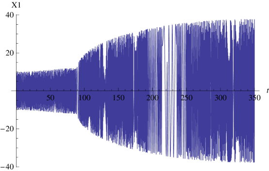
Figure 1: A typical classical trajectory of the Hamiltonian (32).

The Hamiltonian

$$H=\frac{P_{1}^{2}+\Omega_{1}^{2}X_{1}^{2}}{2}-\frac{P_{2}^{2}+\Omega_{2}^{2}X_{2}^{2}}{2}+\lambda(X_{1}-X_{2})(X_{1}+X_{2})^{3}$$ (32)

is a close relative to the supersymmetric Hamiltonian considered in [5]. The bosonic part of the latter is

$$H=pP+D(\Omega^{2}x+\lambda x^{3}),$$ (33)

where $(p,P)$ are the canonical momenta of $(x,D)$. By introducing $X_{1,2}=(x\pm D)/\sqrt{2}$, it is reduced to the Hamiltonian (32) with $\Omega_{1}=\Omega_{2}=\Omega$. The system (33) is integrable and the classical trajectories are expressed analytically into Jacobi elliptic functions. In this case, the amplitude of oscillations grows linearly with time, but this does not represent a disaster as the trajectories do not run into infinity in a finite time. The Schrödinger equation for the Hamiltonian (33) can be solved analytically [5]. The spectrum is continuous, with eigenvalues lying in two intervals $]-\infty,-\Omega]\cup[\Omega,\infty[$ plus the eigenvalue $\{0\}$. The quantum spectrum for the Hamiltonian (32) should have the same qualitative features. Besides (31), there are other interaction potentials providing for the same behaviour. One of them is $V(X_{1},X_{2})=\lambda(X_{1}-X_{2})^{3}(X_{1}+X_{2})$. Note that, being expressed in terms of the original variables $x$, $q$, $p_{x}$, $p_{q}$, the Hamiltonian (32) acquires a rather complicated form and the corresponding Lagrangian depending on $q$ and its time derivatives is even more complicated. Natural nonlinear extensions of the Lagrangian (1) seem all to involve classical and quantum collapse.

5 Complexification

The spectral Sturm–Liouville problem is defined when the operator in question (Hamiltonian) is given and boundary conditions are specified. It is possible thus to have different spectral problems associated with a given Hamiltonian.

Take a simple oscillator,

$$H=\frac{1}{2}(P^{2}+\Omega^{2}X^{2}).$$

If considering the spectral problem at real $X$ and requiring that wave functions vanish at infinity, we obtain the usual spectrum

$$E_{n}=\Omega(n+1/2).$$

The wave functions, $\Psi\propto e^{-X^{2}/2}$, continued analytically to complex $X$, vanish asymptotically not only on the real axis, but in the whole Stokes wedge with $|{\rm arg}(X)|<\pi/4$. Nothing prevents, however, to consider another spectral problem and require that wave functions vanish at large imaginary $X$. The corresponding eigenfunctions are $\Psi_{n}\propto H_{n}(iX)e^{X^{2}/2}$. They vanish in the complementary Stokes wedge as shown in Fig. 2. The spectrum is now

$$E_{n}=-\Omega(n+1/2).$$

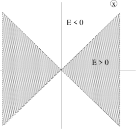
Figure 2: Stokes wedges.

We have seen that the free PU oscillator with different frequencies is equivalent to the combination of two oscillators (5) with the spectrum (6). But the latter is true only if $q$, $x$, $p_{q}$, $p_{x}$ and hence $X_{1,2}$ are assumed to be real. One can on the other hand assume that, while $X_{1}$ is kept real, $X_{2}$ is imaginary. In this case, the sign of the energy eigenvalues of the second oscillator is reversed, and one obtains a positive definite spectrum

$$E_{nm}=\left(n+\frac{1}{2}\right)\Omega_{1}+\left(m+\frac{1}{2}\right)\Omega_{2},\qquad n,m=0,1,\ldots$$ (34)

with no trace of ghosts. Another way to obtain this result is the following [9, 10]. Let us consider the Hamiltonian (2) and assume $x$ being real and $q$ being imaginary there, $q=iy$, $p_{q}=-ip_{y}$. The Hamiltonian acquires the form

$$H=\frac{p_{x}^{2}}{2}-ixp_{y}+\frac{(\Omega_{1}^{2}+\Omega_{2}^{2})x^{2}}{2}+\frac{\Omega_{1}^{2}\Omega_{2}^{2}y^{2}}{2}.$$ (35)

The second term in this expression is complex which may lead to worries whether the Hamiltonian (35) makes sense. This worries are not grounded, however. Though the Hamiltonian (35) is not manifestly Hermitian, it belongs to the class of crypto-Hermitian Hamiltonians with real spectrum [15]. The Hamiltonian (35) can be diagonalized to the manifestly Hermitian form,

$$H_{\rm diag}=\frac{P_{1}^{2}+\Omega_{1}^{2}X_{1}^{2}}{2}+\frac{P_{2}^{2}+\Omega_{2}^{2}X_{2}^{2}}{2}.$$ (36)

by a complex canonical transformation (a brother of the transformation (4)),

$$X_{1}\equiv\tilde{x}=\frac{1}{\Omega}_{1}\frac{\Omega_{1}^{2}x-ip_{y}}{\sqrt{\Omega_{1}^{2}-\Omega_{2}^{2}}},\qquad X_{2}\equiv\tilde{y}=\frac{\Omega_{1}^{2}y-ip_{x}}{\sqrt{\Omega_{1}^{2}-\Omega_{2}^{2}}},$$

$$P_{1}\equiv\tilde{p}_{x}=\Omega_{1}\frac{p_{x}+i\Omega_{2}^{2}y}{\sqrt{\Omega_{1}^{2}-\Omega_{2}^{2}}},\qquad P_{2}\equiv\tilde{p}_{y}=\frac{p_{y}+i\Omega_{2}^{2}x}{\sqrt{\Omega_{1}^{2}-\Omega_{2}^{2}}}.$$ (37)

This transformation amounts to a certain similarity nonunitary transformation,

$$H_{\rm diag}=e^{-S}e^{-R}He^{R}e^{S}$$ (38)

with

$$R=\left(\frac{p_{x}p_{y}}{2\Omega_{1}\Omega_{2}}+\frac{xy\Omega_{1}\Omega_{2}}{2}\right)\ln\frac{\Omega_{1}+\Omega_{2}}{\Omega_{1}-\Omega_{2}},$$

and

$$S=\frac{i\ln\Omega_{1}}{2}(yp_{y}+p_{y}y).$$

To find the eigenfunctions of (35), one can either rotate away the eigenfunctions of (36), $\Psi=e^{R}e^{S}\Psi_{\rm diag}$ or proceed in the same way as in [6] representing the wave functions as

$$\Psi_{nm}=\phi_{nm}\exp\left\{-\frac{\Omega_{1}+\Omega_{2}}{2}(x^{2}+\Omega_{1}\Omega_{2}y^{2})-\Omega_{1}\Omega_{2}xy\right\}.$$

The operator acting on $\phi_{nm}(x,y)$ is

$$\hat{O}=-\frac{1}{2}\frac{\partial^{2}}{\partial x^{2}}-x\frac{\partial}{\partial y}+[x(\Omega_{1}+\Omega_{2})+y\Omega_{1}\Omega_{2}]\frac{\partial}{\partial x}+\frac{\Omega_{1}+\Omega_{2}}{2}.$$

Introducing

$$z=\sqrt{\Omega_{1}}(x+\Omega_{2}y),\qquad w=\sqrt{\Omega_{2}}(x+\Omega_{1}y),$$

it acquires the form

$$\hat{O}=\Omega_{1}\left[-\frac{1}{2}\frac{\partial^{2}}{\partial z^{2}}+z\frac{\partial}{\partial z}\right]+\Omega_{2}\left[-\frac{1}{2}\frac{\partial^{2}}{\partial w^{2}}+w\frac{\partial}{\partial w}\right]-\sqrt{\Omega_{1}\Omega_{2}}\frac{\partial^{2}}{\partial z\partial w}+\frac{\Omega_{1}+\Omega_{2}}{2}.$$ (39)

The eigenfunctions of $\hat{O}$ are polynomials. When the dependence on the variable $w$ or on the variable $z$ is suppressed, they are conventional Hermite polynomials,

$$\phi_{n0}=H_{n}(z),\qquad\phi_{0m}=H_{m}(w).$$

When both $n\neq 0$ and $m\neq 0$, the eigenfunction is

$$\phi_{nm}(x,y)=\sum_{k=0}^{\min(n,m)}\left(-\frac{\Omega_{1}+\Omega_{2}}{4\sqrt{\Omega_{1}\Omega_{2}}}\right)^{k}\frac{m!(n-m)!}{(m-k)!k!(n-m+k)!}H_{n-m+k}(z)H_{k}(w),$$ (40)

The expression (40) is very similar to (8) and is obtained from the latter by substituting $i\Delta=i(\Omega_{1}-\Omega_{2})\to-(\Omega_{1}+\Omega_{2})$ and replacing the arguments $i\sqrt{\Omega_{1}}(\Omega_{2}q-ix)\to z$, $\sqrt{\Omega_{2}}(\Omega_{1}q+ix)\to w$.

There is a price, however, that one has to pay for getting rid of negative energies in the spectrum. The Hamiltonian (35) is not Hermitian and this means that the conventionally defined norm $\|\Psi\|=\iint dxdy\left|\Psi(x,y)\right|^{2}$ is not preserved during evolution. In addition, the eigenfunctions (40) do not represent an orthogonal basis with respect to this norm. True, crypto-Hermiticity of the Hamiltonian implies that a norm with respect to which the evolution is unitary can be defined, but this norm,

$$\|\Psi\|^{\prime}=\langle\Psi^{*}e^{-2R}\Psi\rangle,$$

has a complicated nonlocal structure.

The transformations (37) are singular at $\Omega_{1}=\Omega_{2}$. This suggests that, as it was the case for the standard PU oscillator, the point $\Omega_{1}=\Omega_{2}$ is exceptional also in the nonstandard realization. The emergence of Jordan blocks in this limit was noticed back in [8], but the best way to see that is to follow, as Bender and Mannheim did [10], the approach of [6] and to explore the fate of eigenfunctions (40) in the limit $\Omega_{1}\to\Omega_{2}$.

In this limit, the variables $z$ and $w$ coincide. The eigenfunctions (40) for a given $n+m$ also all coincide in this limit, $\phi_{nm}(z)\sim H_{n+m}(z)$. To derive the latter, note that the operator (39) acquires in the limit $\Omega_{1}\to\Omega_{2}$ the form

$$\hat{O}_{\Omega_{1}=\Omega_{2}}=\Omega\left[-\frac{\partial^{2}}{\partial z^{2}}+2z\frac{\partial}{\partial z}+1\right]$$

and its eigenfunctions are simple Hermite polynomials, indeed. After massaging equation (40) a little bit, we derive, as a byproduct, a nice mathematical identity

$$H_{n+m}(z)=\sum_{j=0}^{\min(n,m)}(-2)^{j}\frac{n!m!}{j!(n-j)!(m-j)!}H_{n-j}(z)H_{m-j}(z).$$

In contrast to the standard PU oscillator where the Jordan blocks had infinite dimension, their dimension is finite here. We have a single vacuum state with energy $E=\Omega$, the Jordan block of dimension 2 at the level $E=2\Omega$, the Jordan block of dimension 3 at the level $E=3\Omega$, etc. At each level, there is a finite number of different nonstationary solutions to the time-dependent Schrödinger equation and one cannot construct, as we did before, bounded in $x,t$ combinations that have the meaning of continuous spectrum wave functions. As a result, unitarity is violated.

As was mentioned, the real problem associated with the ghosts is the quantum and/or classical collapse, which might appear only in interacting theory. It is not so easy to include interactions and analyze their effects in the Bender–Mannheim approach. First, it is not clear whether the Hamiltonian (35) with the interaction term like $\lambda y^{4}$ is still crypto-Hermitian. The canonical transformations (37) [or, which is equivalent, the similarity transformation (38)] kill the complexity $-ixp_{y}$, but bring about new complexities coming from the interaction term $\propto y^{4}$. These complexities have the form $\Delta H_{\rm diag}\propto i\lambda(\Omega_{1}^{2}P_{1}X_{2}^{3}-P_{1}^{3}X_{2})$. We failed to find a modified canonical transformation that would kill all complexities.

Even if one succeeds in finding a nonlinear crypto-Hermitian generalization of the Hamiltonian (35), it would be difficult to analyze its spectrum and to find out whether the ground state is still present there. In particular, it would be difficult to implement variational estimates due to a complicated nonlocal norm.

6 Conclusions

Our main message is that the ghosts (the absence of the ground state in the spectrum), do not represent a serious problem for free theory. Thus, it is not necessary to cope with them there. The spectrum of the free PU oscillator runs from $-\infty$ to $+\infty$ representing a pure point spectrum that is dense everywhere when $\Omega_{1}\neq\Omega_{2}$ and a continuous spectrum when $\Omega_{1}=\Omega_{2}$. The latter can also be interpreted via infinite-dimensional Jordan blocks that appear in the limit $\Omega_{1}\to\Omega_{2}$ [6]. In spite of the absence of the ground state, unitarity is preserved.

Generically, interactions break unitarity due to quantum collapse phenomenon. However, there are certain special cases when the theory involves neither classical nor quantum collapse. A particularly interesting example is the exactly soluble nonlinear Hamiltonian (33) that appears in the context of supersymmetric higher derivative quantum mechanics [5].

By analytical continuation to complex coordinates, it is possible to consider a nonstandard realization of the free PU Hamiltonian with the positive definite spectrum (34). When $\Omega_{1}\neq\Omega_{2}$, a unitary evolution operator can be defined. The presence of the ground state may be considered as a certain advantage of this realization compared to the standard one. However,

1. It is misleading to say that choosing the nonstandard realization “solves the ghost problem”. The analysis has been performed only for free theory and, in the free case, there is no serious problem to solve anyway.

2. In contrast to the standard one, the nonstandard PU oscillator at equal frequencies is not unitary.

3. As far as the original problem with the Lagrangian (1) is concerned, the nonstandard realization does not look natural: (i) it is not so natural to assume that the coordinate $q$ is imaginary while its time derivative $x=\dot{q}$ is real; (ii) the norm in the space $(y\equiv-iq,\ x)$ that is preserved during evolution has a complicated nonlocal structure.

4. It is not known yet what happens in the framework of nonstandard realization when interactions are included.

Acknowledgements

I acknowledge warm hospitality at AEI in Golm, where this work was finished and thank P. Mannheim for useful correspondence.

References

- [1]
- [2] Smilga A.V., 6D superconformal theory as the theory of everything, in Gribov Memorial Volume, Editors Yu.L. Dokshitzer, P. Levai and J. Nyiri, World Scientific, 2006, 443–459, hep-th/0509022.
- [3] Smilga A.V., Benign versus malicious ghosts in higher-derivative theories, Nuclear Phys. B 706 (2005), 598–614, hep-th/0407231.
- [4] Pais A., Uhlenbeck G.E., On field theories with nonlocalized action, Phys. Rev. 79 (1950), 145–165.
- [5] Robert D., Smilga A.V., Supersymmetry versus ghosts, J. Math. Phys. 49 (2008), 042104, 20 pages, math-ph/0611023.
- [6] Smilga A.V., Ghost-free higher-derivative theory, Phys. Lett. B 632 (2006), 433–438, hep-th/0503213.
- [7] Bolonek K., Kosinski P., Comments on “Dirac quantization of Pais–Uhlenbeck fourth order oscillator”, quant-ph/0612009.
- [8] Mannheim P.D., Davidson A., Dirac quantization of the Pais–Uhlenbeck fourth order oscillator, Phys. Rev. A 71 (2005), 042110, 9 pages, hep-th/0408104.
- [9] Bender C.M., Mannheim P.D., No ghost theorem for the fourth-order derivative Pais–Uhlenbeck oscillator model, Phys. Rev. Lett. 100 (2008), 110402, 4 pages, arXiv:0706.0207.
- [10] Bender C.M., Mannheim P.D., Exactly solvable PT-symmetric Hamiltonian having no Hermitian counterpart, Phys. Rev. D 78 (2008), 025022, 20 pages, arXiv:0804.4190.
- [11] Ostrogradsky M., Mémoires sur les équations différentielles relatives au problème des isopérimètres, Mem. Acad. St. Petersbourg, VI 4 (1850), 385–517.
- [12] Heiss W.D., Exceptional points of non-Hermitian operators, J. Phys. A: Math. Gen. 37 (2004) 2455–2464, quant-ph/0304152.
- [13] Anderson A., Canonical transformations in quantum mechanics, Ann. Phys. 232 (1994) 292–331, hep-th/9305054.
-
[14]
Case K.M., Singular potentials, Phys. Rev. 80 (1950), 797–806.
Meetz K., Singular potentials in non-relativistic quantum mechanics, Nuovo Cimento 34 (1964), 690–708.
Perelomov A.M., Popov V.S., Collapse onto scattering center in quantum mechanics, Teor. Mat. Fiz. 4 (1970), 48–65. -
[15]
Bronzan J.B., Shapiro J.A., Sugar R.L., Reggeon field theory in zero transverse dimensions, Phys. Rev. D 14 (1976), 618–631.
Amati D., Le Bellac M., Marchesini G., Ciafaloni M., Reggeon field theory for , Nuclear Phys. B 112 (1976), 107–149.
Gasymov M.G., Spectral analysis of a class of second-order non-self-adjoint differential operators, Funktsional. Anal. i Prilozhen. 14 (1980), 14–19.
Caliceti E., Graffi S., Maioli M., Perturbation theory of odd anharmonic oscillators, Comm. Math. Phys. 75 (1980), 51–66.
Scholtz F.G., Geyer H.B., Hahne F.J.W., Quasi-Hermitian operators in quantum mechanics and the variational principle, Ann. Physics 213 (1992), 74–101.
Bender C.M., Boettcher S., Real spectra in non-Hermitian Hamiltonians having PT symmetry, Phys. Rev. Lett. 80 (1998), 5243–5246, physics/9712001.
Mostafazadeh A., PT-symmetric cubic anharmonic oscillator as a physical model, J. Phys. A: Math. Gen. 38 (2005), 6557–6570, quant-ph/0411137.\LastPageEnding