Multi-Harnack smoothings of real plane branches

Introduction

The 16th problem of Hilbert addresses the determination and the understanding of the possible topological types of smooth real algebraic curves of a given degree in the projective plane $\mathbf{R}P^{2}$. This paper is concerned with a local version of this problem: given a germ $(C,0)$ of real algebraic plane curve singularity, determine the possible topological types of the smoothings of $C$. A smoothing of $C$ is a real analytic family $C_{t}\subset B$, for $t\in[0,1]$, such that $C_{0}=C$ and $C_{t}$ is non singular and transversal to the boundary of a Milnor ball $B$ of the singularity $(C,0)$ for $0<t\ll 1$. In this case the real part $\mathbf{R}C_{t}$ of $C_{t}$ consists of finitely many ovals and non closed components in the Milnor ball.

In the algebraic case it was shown by Harnack that a real projective curve of degree $d$ has at most $\frac{1}{2}(d-1)(d-2)+1$ connected components. A curve with this number of components is called a $M$-curve. In the local case there is a similar bound, depending on the number of real branches of the singularity (see Section 5.1), which arises from the application of the classical topological theory of Smith. A smoothing which reaches this bound on the number of connected components is called a $M$-smoothing. It should be noticed that in the local case $M$-smoothings do not always exists (see [K-O-S]). One relevant open problem in the theory is to determine the actual maximal number of components of a smoothing of $(C,0)$, for $C$ running in a suitable form of equisingularity class refining the classical notion of Zariski of equisingularity class in the complex world (see [K-R-S]).

Quite recently Mikhalkin has proved a beautiful topological rigidity property of those $M$-curves in $\mathbf{R}P^{2}$ which are embedded in maximal position with respect to the coordinate lines (see [M]). His result, which holds more generally, for those $M$-curves in projective toric surfaces which are cyclically in maximal position with respect to the toric coordinate lines, is proved by analyzing the topological properties of the associated amoebas. The amoeba of a curve $C$ is the image of the points $(x,y)\in(\mathbf{C}^{*})^{2}$ in the curve by the map $Log:(\mathbf{C}^{*})^{2}\rightarrow\mathbf{R}^{2}$, given by $(x,y)\mapsto(\log|x|,\log|y|)$. Conceptually, the amoebas are intermediate objects which lay in between classical algebraic curves and tropical curves. See [F-P-T], [G-K-Z], [M], [M-R], [P-R] and [I1] for more on this notion and its applications.

In this paper we study smoothings of a real plane branch singularity $(C,0)$, i.e., the germ $(C,0)$ is analytically irreducible in $(\mathbf{C}^{2},0)$ and admits a real Newton-Puiseux parametrization. Risler proved that any such germ $(C,0)$ admits a $M$-smoothing with the maximal number ovals, namely $\frac{1}{2}\mu(C)_{0}$, where $\mu$ denotes the Milnor number. The technique used, called nowadays the blow-up method, is a generalization of the classical Harnack construction of $M$-curves by small perturbations, using the components of the exceptional divisor as a basis of rank one (see [R2], [K-R] and [K-R-S]). One of our motivations was to study to which extent Mikhalkin’s result holds for smoothings of singular points of real plane curves, particularly for Harnack smoothings, those $M$-smoothings which are in maximal position with respect to two coordinates lines through the singular point.

We develop a new construction of smoothings of a real plane branch $(C,0)$ by using Viro Patchworking method. Since real plane branches are Newton degenerated, we cannot apply Viro Patchworking method directly. Instead we apply the Patchworking method for certain Newton non degenerate curve singularities with several branches which are defined by semi-quasi-homogeneous polynomials. These singularities appear as a result of iterating deformations of the strict transforms $(C^{(j)},o_{j})$, at certain infinitely near points $o_{j}$ of the embedded resolution of singularities of $(C,0)$. Our method yields multi-parametric deformations, which we call multi-semi-quasi-homogeneous (msqh) and provides simultaneously msqh-smoothings of the strict transforms $(C^{(j)},o_{j})$. We exhibit suitable hypothesis which characterize $M$-smoothings and Harnack smoothings for this class of deformations (see Theorem 8.1). Up to the author’s knowledge, Theorem 8.1 is the first instance in the literature in which Viro Patchoworking method is used to define smoothings of Newton degenerated singularities, with controlled topology.

We introduce the notion of multi-Harnack smoothings, those Harnack smoothings, such that the msqh-$M$-smoothings of the strict transforms $C^{(j)}$ appearing in the process are Harnack. We prove that any real plane branch $C$ admits a multi-Harnack smoothing. For this purpose we prove the existence of Harnack smoothings of singularities defined by certain semi-quasi-homogeneous polynomials (see Proposition 6.4). One of our main results, Theorem 8.4, states that multi-Harnack smoothings of a real plane branch $(C,0)$ have a unique topological type, which depends only on the complex equisingular class of $(C,0)$. In particular, multi-Harnack smoothings do not have nested ovals. Theorem 8.4 can be understood as a local version of Mikhalkin’s Theorem 4.1. The proof is based on Theorem 8.1 and an extension of Mikhalkin’s result for Harnack smoothings of certain non-degenerated singular points (Theorem 6.1).

We also analyze certain multi-scaled regions containing the ovals. The phenomena is quite analog to the analysis of the asymptotic concentration of the curvature of the Milnor fibers in the complex case, due to García Barroso and Teissier [GB-T].

It is a challenge for the future to extend, as possible, the techniques and results of this paper to the constructions of smoothings of other singular points of real plane curves.

The paper is organized as follows. The five first sections are preliminary material: in Sections 1, 2 and 3 we introduce the Viro Patchworking method, also in the toric context; we recall Mikhalkin’s result on Harnack curves in projective toric surfaces in Section 4; the notion of smoothings of real plane curve singular points is presented in section 5. Section 6 contains the first new results, in particular, the determination of the topological type of Harnack smoothings of singularities defined by certain non degenerated semi-quasi-homogeneous polynomials (see Theorem 6.1). In Section 7 we recall the construction of a toric resolution of a plane branch and we introduce the support of the msqh-smoothings, which are studied in the last section. The main results of the paper are collected in Section 8: the characterization of maximal, Harnack and multi-Harnack-msqh-smoothings in Theorem 8.1 and Corollary 8.2, and the characterization of the topological type of multi-Harnack smoothings in Theorem 8.4, the description of the scales of ovals in Section 8.5 and finally some examples explained in detail.

1. Basic notations and definitions

A real algebraic variety is a complex algebraic variety $V$ invariant by an anti-holomorphic involution, we denote by $\mathbf{R}V$ the real part. For instance, a real algebraic plane curve $C\subset\mathbf{C}^{2}$ is a complex plane curve which is invariant under complex conjugation. The curve $C$ is defined by $P=0$ where $0\neq P=\sum c_{i,j}x^{i}y^{j}\in\mathbf{R}[x,y]$. We use the following notations and definitions:

The Newton polygon of $P$ (resp. the local Newton polygon) is the convex hull in $\mathbf{R}^{2}$ of the set $\{(i,j)\mid c_{i,j}\neq 0\}$ (resp. of $\{(i,j)+\mathbf{R}^{2}_{\geq 0}\mid c_{i,j}\neq 0\}$).

If $\Lambda\subset\mathbf{R}^{2}$ we denote by $P^{\Lambda}$ the symbolic restriction $P^{\Lambda}:=\sum_{(i,j)\in\Lambda\cap\mathbf{Z}^{2}}c_{i,j}x^{i}y^{j}$.

Suppose that $0\in C\subset\mathbf{C}^{2}$ is an isolated singular point of $C$ and that $C$ does not contain a coordinate axis. Then the Newton diagram of $P$ is the closed region $\Delta$ bounded by the coordinate axis and the local Newton polygon of $P$.

The polynomial $P$ is non degenerated (resp. real non degenerated) with respect to its Newton polygon if for any compact face $\Theta$ of it we have that $P^{\Theta}=0$ defines a non singular subset of $(\mathbf{C}^{*})^{2}$ (resp. of $(\mathbf{R}^{*})^{2}$). In this case if $\Lambda$ is an edge of the Newton polygon of $P$, then the polynomial $P^{\Lambda}$ is of the form:

(1) $$P^{\Lambda}=cx^{a}y^{b}\prod_{i=1}^{e}(y^{n}-\alpha_{i}x^{m}),$$

where $c\neq 0$, $a,b\in\mathbf{Z}_{\geq 0}$, the integers $n,m\geq 0$ are coprime and the numbers $\alpha_{1},\dots,\alpha_{e}\in\mathbf{C}^{*}$, which are called peripheral roots of $P$ along the edge $\Lambda$ or simply peripheral roots of $P^{\Lambda}$, are distinct (resp. the real peripheral roots of $P^{\Lambda}$ are distinct). Notice that the non degeneracy (resp. real non degeneracy) of $P$ implies that $C\cap(\mathbf{C}^{*})^{2}$ is non singular (resp. $C\cap(\mathbf{R}^{*})^{2}$), for taking $\Theta$ equal to the Newton polygon of $P$ in the definition.

We say that $P$ is non degenerated (resp. real non degenerated) with respect to its local Newton polygon if for any edge $\Lambda$ of it we have that the equation $P^{\Lambda}=0$ defines a non singular subset of $(\mathbf{C}^{*})^{2}$ (resp. of $(\mathbf{R}^{*})^{2}$).

The notion of non degeneracy with respect to the Newton polyhedra extend for polynomials of more than two variables (see [Kou]).

2. The real part of a projective toric variety

We introduce basic notations and facts on the geometry of toric varieties. We refer the reader to [G-K-Z], [Od] and [Fu] for proofs and more general statements. For simplicity we state the notations only for surfaces.

Let $\Theta$ be a convex two dimensional polytope in $\mathbf{R}^{2}_{\geq 0}$ with integral vertices, a polygon in what follows. We associate to the polygon $\Theta$ a projective toric variety $Z(\Theta)$. The algebraic torus $(\mathbf{C}^{*})^{2}$ is embedded as an open set of $Z(\Theta)$, and acts on $Z(\Theta)$, in a way which coincides with the group operation on the torus. There is a one to one correspondence between the faces of $\Theta$ and the orbits of the torus action, which preserves the dimensions and the inclusions of the closures. If $\Lambda$ is a one dimensional face of $\Theta$, we have an embedding $Z(\Lambda)\subset Z(\Theta)$. The variety $Z(\Lambda)$ is a projective line $\mathbf{C}P^{1}$ embedded in $Z(\Theta)$. These lines are called the coordinate lines of $Z(\Theta)$. The intersection of two coordinate lines $Z(\Lambda_{1})$ and $Z(\Lambda_{2})$ reduces to a point (resp. is empty) if and only if the edges $\Lambda_{1}$ and $\Lambda_{2}$ intersect in a vertex of $\Theta$ (resp. otherwise). The surface $Z(\Theta)$ may have singular points only at the zero-dimensional orbits. The algebraic real torus $(\mathbf{R}^{*})^{2}$ is an open subset of the real part $\mathbf{R}Z(\Theta)$ of $Z(\Theta)$ and acts on it. The orbits of this action are just the real parts of the orbits for the complex algebraic torus action. For instance if $\Theta$ the simplex with vertices $(0,0)$, $(0,d)$ and $(d,0)$ then the surface $Z(\Theta)$ with its coordinate lines is the complex projective plane with the classical three coordinate axis.

The image of the moment map $\phi_{\Theta}:(\mathbf{C}^{*})^{2}\rightarrow\mathbf{R}^{2}$,

(2) $$(x,y)\mapsto\left(\sum_{\alpha_{k}={(i,j)},\alpha_{k}\in\Theta\cap\mathbf{Z}^{2}}|x^{i}y^{j}|\right)^{-1}\left(\sum_{\alpha_{k}={(i,j)},\alpha_{k}\in\Theta\cap\mathbf{Z}^{2}}|x^{i}y^{j}|(i,j)\right).$$

is $\mbox{{\rm int}}\Theta$, where int denotes relative interior. The restriction $\phi_{\Theta}^{+}:=\phi_{\Theta|\mathbf{R}^{2}_{>0}}$ is a diffeomorphism of $\mathbf{R}^{2}_{>0}$ onto the interior of $\Theta$.

Denote by ${\mathcal{S}}\cong(\mathbf{Z}/2\mathbf{Z})^{2}$ the group consisting of the orthogonal symmetries of $\mathbf{R}^{2}$ with respect to the coordinate lines, namely the elements of ${\mathcal{S}}$ are $\rho_{i,j}:\mathbf{R}^{2}\rightarrow\mathbf{R}^{2}$, where $\rho_{i,j}(x,y)=((-1)^{i}x,(-1)^{j}y)$ for $(i,j)\in\mathbf{Z}^{2}_{2}$.

If $A\subset\mathbf{R}^{2}$ we denote by $\tilde{A}$ the union $\tilde{A}:={\bigcup_{\rho\in{\mathcal{S}}}}\,\rho(A)\subset\mathbf{R}^{2}$.

The map $\phi_{\Theta}^{+}$ extends to a diffeomorphism: $\tilde{\phi}_{\Theta}:(\mathbf{R}^{*})^{2}\rightarrow\widetilde{\mbox{{\rm int}}{({\Theta})}}$ by $\tilde{\phi}_{\Theta}(\rho(x)):=\rho(\phi(x))$, for $x\in\mathbf{R}^{2}_{>0}$ and $\rho\in{\mathcal{S}}$.

If $\Lambda$ is an edge of $\Theta$ and if $n=(u,v)$ is a primitive integral vector orthogonal to $\Lambda$ we denote by $\rho_{\Lambda}$ or by $\rho_{\Lambda}(a,b)$ the element of ${\mathcal{S}}$ defined by $\rho_{\Lambda}(a,b)=((-1)^{u}a,(-1)^{v}b)$.

We consider the equivalence relation $\sim$ in the set $\tilde{\Theta}$, which for each edge $\Lambda$ of $\Theta$, identifies a point in $\Lambda$ with its symmetric image by $\rho_{\Lambda}$. Set $\tilde{\Lambda}/\sim$ the image of $\tilde{\Lambda}$ in $\tilde{\Theta}/\sim$. For each edge $\Lambda$ of $\Theta$ we have diffeomorphisms ${\phi}_{\Lambda}^{+}:\mathbf{R}_{>0}\rightarrow\mbox{\rm int}{\Lambda}$ and $\tilde{\phi}_{\Lambda}:\mathbf{R}^{*}\rightarrow\widetilde{\mbox{\rm int}{\Lambda}}/\sim$, corresponding to the moment map in the one dimensional case. Notice that $\widetilde{\mbox{\rm int}{\Lambda}}/\sim$ has two connected components and the real part $\mathbf{R}Z(\Lambda)$ corresponds to $\tilde{\Lambda}/\sim$.

We summarize this constructions in the following result (see [Od] Proposition 1.8 and [G-K-Z], Chapter 11, Theorem 5.4 for more details and precise statements).

Proposition 2.1.

The morphisms defined from the moment map glue up ia a stratified homeomorphism

(3) $$\begin{array}[]{cccc}\Psi_{\Theta}:&\tilde{\Theta}/\sim&\longrightarrow&\mathbf{R}Z(\Theta),\end{array}$$

which for any edge $\Lambda$ of $\Theta$ applies $\tilde{\Gamma}/\sim$ to the correspondent coordinate line $\mathbf{R}Z(\Lambda)\subset\mathbf{R}Z(\Theta)$. The composite

$$\begin{array}[]{ccccccc}(\mathbf{R}^{*})^{2}&\stackrel{{\scriptstyle\tilde{\phi}_{\Theta}}}{{\longrightarrow}}&\tilde{\Theta}&\longrightarrow&\tilde{\Theta}/\sim&\stackrel{{\scriptstyle\Psi_{\Theta}}}{{\longrightarrow}}&\mathbf{R}Z(\Theta).\end{array}$$

is the inclusion of the real part of the torus in $\mathbf{R}Z(\Theta)$.

A polynomial $P\in\mathbf{R}[x,y]$ with Newton polygon equal to $\Theta$ defines a real algebraic curve $C$ in the real toric surface $Z(\Theta)$ which does not pass through any $0$-dimensional orbit. If $C$ is smooth its genus coincides with the number of integral points in the interior of $\Theta$, see [Kh]. The curve $C$ is a $M$-curve if $\mathbf{R}C$ has the maximal number $1+\#\mbox{{\rm int}}{\Theta}\cap\mathbf{Z}^{2}$ of connected components. If $\Lambda$ is an edge of $\Theta$ the intersection of $C$ with the coordinate line $Z(\Lambda)$ is defined by $P^{\Lambda}$. The number of zeroes of $P^{\Lambda}$ in the projective line $Z(\Lambda)$, counted with multiplicity, is equal to the integral length of the segment $\Lambda$, i.e., one plus the number of integral points in the interior of $\Lambda$. This holds since these zeroes are the image of the peripheral roots $\alpha_{i}$ of $P^{\Lambda}$ (see (1)) by the embedding map $\mathbf{C}^{*}\hookrightarrow Z(\Lambda)$. For this reason we abuse sometimes of terminology and call peripheral roots the zeroes of $P^{\Lambda}$ in the projective line $Z(\Lambda)$.

3. Patchworking real algebraic curves

Patchworking is a method introduced by Viro for constructing real algebraic hypersurfaces (see [V1], [V4] [V2], [V3] and [I-V], see also [G-K-Z] and [R1] for an exposition and [B] and [St] for some generalizations). We use the Notations introduced in Section 2.

Let $\Theta\subset\mathbf{R}^{2}_{\geq 0}$ be an integral polygon. The following definition is fundamental.

Definition 3.1.

Let $Q\in\mathbf{R}[x,y]$ define a real algebraic curve $C$ then the $\Theta$-chart $\mbox{\rm Ch}_{\Theta}(C)$ of $C$ is the closure of $\mbox{\rm Ch}_{\Theta}^{*}(C):=\tilde{\phi}_{\Theta}(\mathbf{R}C\cap(\mathbf{R}^{*})^{2})$ in $\tilde{\Theta}$.

If $\Theta$ is the Newton polygon of $Q$ we often denote $\mbox{\rm Ch}_{\Theta}(C)$ by $\mbox{\rm Ch}(Q)$ or by $\mbox{\rm Ch}(C)$ if the coordinates used are clear from the context. If $Q$ is real non degenerated with respect its Newton polygon, then for any face $\Lambda$ of $\Theta$ we have that $\mbox{\rm Ch}_{\Theta}(Q)\cap\tilde{\Lambda}=\mbox{\rm Ch}_{\Lambda}(Q_{\Lambda})$ and the intersection $\mbox{\rm Ch}_{\Theta}(Q)\cap\tilde{\Lambda}$ is transversal (as stratified sets).

Notation 3.2.

We consider a polynomial $P_{t}=\sum A_{i,j}(t)x^{i}y^{j}\in\mathbf{R}[t,x,y]$, as a family of polynomials in $\mathbf{R}[x,y]$.

1. We denote by $\Theta\subset\mathbf{R}^{2}$ the Newton polygon of $P_{t}$, when $0<t\ll 1$.

2. We denote by $\hat{\Theta}\subset\mathbf{R}\times\mathbf{R}^{2}$ the Newton polytope of $P_{t}$, when it is viewed as a polynomial in $\mathbf{R}[t,x,y]$.

3. We denote by $\hat{\Theta}_{c}$ the lower part of $\hat{\Theta}$, i.e., the union of compact faces of the Minkowski sum $\hat{\Theta}+(\mathbf{R}_{\geq 0}\times\{(0,0)\})$.

4. The restriction of the second projection $\mathbf{R}\times\mathbf{R}^{2}\rightarrow\mathbf{R}^{2}$ to $\hat{\Theta}_{c}$ induces a finite strictly convex polyhedral subdivision $\Theta^{\prime}$ of $\Theta$. The inverse function $\omega:\Theta\rightarrow\hat{\Theta}_{c}$ is a piece-wise affine strictly convex function. Any cell $\Lambda$ of the subdivision $\Theta^{\prime}$ corresponds by this function to a face $\hat{\Lambda}$ of $\hat{\Theta}$ contained in $\hat{\Theta}_{c}$, of the same dimension, and the converse also holds. The Newton polygon of $P_{0}$ is a face of $\Theta^{\prime}$ by construction.

5. If $\Lambda$ is a cell of $\Theta^{\prime}$ we denote by $P^{\hat{\Lambda}}_{1}$, or by $P^{\hat{\Lambda}}_{t=1}$ the polynomial in $\mathbf{R}[x,y]$ obtained by substituting $t=1$ in $P_{t}^{\hat{\Lambda}}$.

Theorem 3.1.

With the above notations, if for each face $\hat{\Lambda}$ of $\hat{\Theta}$ contained in $\hat{\Theta}_{c}$ the polynomial $P^{\hat{\Lambda}}_{{1}}$ is real non degenerated with respect to ${\Lambda}$, then the pair $(\tilde{\Theta},\mbox{\rm Ch}_{\Theta}(P_{t}))$ is stratified homeomorphic to $(\tilde{\Theta},\tilde{C})$, where $\tilde{C}$ is the curve obtained by gluing together in $\tilde{\Theta}$ the charts $\mbox{\rm Ch}_{\Lambda}(P^{\hat{\Lambda}}_{{1}})$ for $\Lambda$ running through the cells of the subdivision $\Theta^{\prime}$, for $0<t\ll 1$.

Remark 3.3.

The statement of Theorem 3.1 above is a slight generalization of the original result of Viro in which the deformation is of the form $\sum A_{i,j}t^{\omega(i,j)}x^{i}y^{j}$, for some real coefficients $A_{i,j}$. The same proof generalize without relevant changes to the case presented here, when we may add terms $B_{k,i,j}t^{k}x^{i}y^{j}$ with $B_{k,i,j}\in\mathbf{R}$ and exponents $(k,i,j)$ contained in $(\hat{\Theta}+\mathbf{R}_{\geq 0}\times\{0\})\setminus\hat{\Theta}_{c}$.

Remark 3.4.

Theorem 3.1 extends naturally to provide constructions of real algebraic curves with prescribed topology in the real toric surface $Z(\Theta)$. The chart $\mbox{Ch}_{\tilde{\Theta}/\sim}(C)$ of the curve $C$ in $Z(\Theta)$ is defined as the closure of $\mbox{Ch}^{*}_{\Theta}(C)$ in $\tilde{\Theta}/\sim$ (where $\sim$ is the equivalence relation defined in Section 2). Then the statement of Theorem 3.1 holds for the curve $C_{t}$ defined by $P_{t}$ in $Z(\Theta)$ by identifying $\tilde{\Theta}/\sim$ and $\mathbf{R}Z(\Theta)$ by the map $\Psi_{\Theta}$ (see (3)).

Definition 3.5.

The gluing of charts of Theorem 3.1 is called combinatorial patchworking if the subdivision $\Theta^{\prime}$ is a primitive triangulation of $\Theta$, i.e., it contains all integral points of $\Theta$ as vertices.

Notice that $\Theta^{\prime}$ is a primitive triangulation if the two dimensional cells $\Lambda$ are primitive triangles, i.e., of area $1/2$ with respect to the standard volume form induced by a basis of the lattice $\mathbf{Z}^{2}$. The description of the charts of a combinatorial patchworking is determined by the subdivision $\Theta^{\prime}$ and the signs of the terms appearing in $P_{t}^{\hat{\Theta}_{c}}$ as a polynomial in $x$ and $y$. The distribution of signs $\epsilon:\Theta\cap\mathbf{Z}^{2}\rightarrow\{\pm 1\}$, induced by taking the signs of the terms appearing in $P_{t}^{\hat{\Theta}_{c}}$, extends to

(4) $$\tilde{\epsilon}:\tilde{\Theta}\cap\mathbf{Z}^{2}\rightarrow\{\pm 1\},\mbox{ by setting }\tilde{\epsilon}(r,s)=(-1)^{i+j}\epsilon\circ\rho_{i,j}(r,s)\mbox{ whenever }\rho_{i,j}(r,s)\in\mathbf{Z}^{2}_{\geq 0}.$$

The chart associated to the polynomial $P_{t}$ in a triangle is empty if all the signs are equal and otherwise is isotopic to segment dividing the triangle in two parts, each one containing only vertices of the same sign. See [G-K-Z], [I-V], [I2].

4. Maximal and Harnack curves in projective toric surfaces

If $C$ is a smooth real projective curve of degree $d$ then the classical Harnack inequality states that the number of connected components of its real part $\mathbf{R}C\subset\mathbf{R}P^{2}$ is bounded by $\frac{1}{2}(d-1)(d-2)+1$. The curve $C$ is called maximal or $M$-curve if the number of components is equal to the bound. Maximal curves always exists and geometric constructions of such curves were found in particular by Harnack, Hilbert and Brusotti. Determining the possible topological types of the pairs $(\mathbf{R}C,\mathbf{R}P^{2})$ in terms of the degree $d$ is usually called the first part of the Hilbert’s 16th problem.

Definition 4.1.

A real projective curve $C$ of degree d is in

1. maximal position with respect to a real line $L$ if the intersection $L\cap C$ is transversal, $L\cap C=\mathbf{R}L\cap\mathbf{R}C$ and $L\cap C$ is contained in one connected component of $\mathbf{R}C$.

2. maximal position with respect to real lines $L_{1},\dots,L_{n}$ in $\mathbf{C}P^{2}$ if $C$ is in maximal position with respect to $L_{i}$, and there exist $n$ disjoint arcs $\mathbf{a}_{1},\dots,\mathbf{a}_{n}$ contained in one connected component of $\mathbf{R}C$ such that $C\cap L_{i}=\mathbf{a}_{i}\cap\mathbf{R}L_{i}$, for $i=1,\dots,n$.

Mikhalkin studied the topological types of the triples $(\mathbf{R}P^{2},\mathbf{R}C,\mathbf{R}L_{1}\cup\dots\cup\mathbf{R}L_{n})$ for those $M$-curves $C$ in maximal position with respect to lines $L_{1},\dots,L_{n}$. He proved that for $n=3$ there is a unique topological type, while for $n>3$ there is none. For $n=1$ the classification reduces to the topological classification of maximal curves in the real affine plane (which is open for $d>5$), while for $n=2$ there are several constructions of $M$-curves of degree $d$, which were found by Brusotti, with $d\geq 4$. See [Br] and [M].

Mikhalkin’s results were stated and proved more generally for real algebraic curves in projective toric surfaces. We denote by $L_{1},\dots,L_{m}$ the sequence of cyclically incident coordinate lines in the toric surface $Z(\Theta)$ associated to the polygon $\Theta$. The notion of maximal position of a real algebraic curve $C\subset Z(\Theta)$ with respect one line is the same as in the projective case.

Definition 4.2.

A real algebraic curve $C$ in the toric surface $Z(\Theta)$ is in maximal position with respect to lines $L_{1},\dots,L_{n}$, for $1\leq n\leq m$, if there exist $n$ disjoint arcs $\mathbf{a}_{1},\dots,\mathbf{a}_{n}$ contained in one connected component of $\mathbf{R}C$ such that the intersection $C\cap L_{i}$ is transversal and contained in $\mathbf{a}_{i}\cap\mathbf{R}L_{i}$, while $\mathbf{a}_{i}\cap\mathbf{R}L_{j}=\emptyset$ if $i\neq j$, for $i=1,\dots,n$ and $j=1,\dots,m$. In addition, we say that:

1. The curve $C$ is cyclically in maximal position if it is in maximal position with respect to the lines $L_{1},\dots,L_{m}$ and the points of intersection of $\mathbf{R}C$ with the lines $L_{1},\dots,L_{m}$ when viewed in the connected component of $\mathbf{R}C$ are partially ordered, following the adjacency of the lines $L_{1},\dots,L_{m}$ .

2. The curve $C$ has good oscillation with respect to the line $L_{i}$ if the points of intersection of $C$ with $L_{i}$ have the same order when viewed in the arc $\mathbf{a}_{i}$ and in the line $\mathbf{R}L_{i}$.

Remark 4.3.

If $C\subset Z(\Theta)$ is in maximal position with respect to the coordinate line $L=Z(\Gamma)$, for $\Gamma$ an edge of $\Theta$, we say also that the chart $\mbox{\rm Ch}_{\Theta/\sim}(C)$ is in maximal position with respect to $\tilde{\Gamma}/\sim$ (see Proposition 2.1).

We have the following result of Mikhalkin (see [M]).

Theorem 4.1.

With the above notations if a $M$-curve $C$ is cyclically in maximal position with respect to the coordinate lines $L_{1},\dots,L_{m}$ of the real toric surface $Z(\Theta)$ then the topological type of the triple $(\mathbf{R}C,\mathbf{R}Z(\Theta),(\mathbf{R}^{*})^{2})$ depends only on $\Theta$.

Definition 4.4.

A Harnack curve in the real toric surface $Z(\Theta)$ is a real algebraic curve $C$ verifying the conclusion of Theorem 4.1.

Remark 4.5.

1. The notion of Harnack curve in this case depends on the polygon $\Theta$. Changing $\Theta$ by $k\Theta$, for $k>1$ provides the same toric variety but the corresponding Harnack curves are different.

2. By our convention and the definitions, the Newton polygon of a polynomial $P\in\mathbf{R}[x,y]$, defining a Harnack curve $C\subset Z(\Theta)$ is equal to $\Theta$. Notice also that $P$ is non degenerated with respect to $\Theta$ and for any edge $\Lambda$ of $\Theta$ the peripheral roots of $P$ along the edge $\Lambda$ are real and of the same sign (see (1)).

If $C$ defines a Harnack curve in $Z(\Theta)$ we denote by $\Omega_{C}$ the unique connected component of $\mathbf{R}C$ which intersects the coordinate lines and by $U_{C}$ the set $\cup{B}_{k}$, where $B_{k}$ runs through the connected components of the set $(\mathbf{R}^{*})^{2}\setminus\Omega_{C}$, whose boundary meets at most two coordinate lines. The set $U_{C}$ is an open region bounding $\Omega_{C}$ and the coordinate lines of the toric surface.

The following Proposition, which is a reformulation of the results of Mikhalkin [M], describes completely the topological type of the real part of a Harnack curve in a toric surface. See Figure 3 below an example.

Proposition 4.6.

With the previous notations, if $C$ defines a Harnack curve in $Z(\Theta)$ then $C$ is cyclically in maximal position with good oscillation with respect to the coordinate lines of the toric surface $Z(\Theta)$. Moreover, the set of connected components of $\mathbf{R}C\cap(\mathbf{R}^{*})^{2}$ can be labelled as $\{\Omega_{r,s}\}_{(r,s)\in\Theta\cap\mathbf{Z}^{2}}$ in such a way that:

- there exists a unique $(i,j)\in\mathbf{Z}^{2}_{2}$ such that for any $(r,s)\in\Theta\cap Z^{2}$:

(5) $$\Omega_{r,s}\subset\rho_{i,j}(\mathbf{R}^{2}_{s,r}).$$

- the set of components $\{\Omega_{r,s}\}_{(r,s)\in\mbox{{\rm\small int}}\Theta}$ consists of non nested ovals in $(\mathbf{R}^{*})^{2}\setminus U_{C}$.

- if $(r,s),(r^{\prime},s^{\prime})\in\partial\Theta\cap\mathbf{Z}^{2}$ then the intersection of closures $\overline{\Omega}_{(r,s)}\cap\overline{\Omega}_{(r^{\prime},s^{\prime})}$ reduces to a point in $Z(\Lambda)$ if and only if $(r,s)$ and $(r^{\prime},s^{\prime})$ are consecutive integral points in $\Lambda$ for some edge $\Lambda$ of $\Theta$, or it is empty otherwise.

- we have that $\Omega_{C}=\bigcup_{(r,s)\in\partial\Theta\cap\mathbf{Z}^{2}}\overline{\Omega}_{r,s}$.

The following Proposition describes the construction of Harnack curve in the real toric surface $Z(\Theta)$ by using combinatorial patchworking (see [I2] Proposition 3.1 and [M] Corollary A4).

Definition 4.7.

Denote by $\epsilon_{h}:\mathbf{Z}^{2}\rightarrow\{\pm 1\}$ the function $\epsilon_{h}(r,s)=(-1)^{(r-1)(s-1)}$. A Harnack distribution of signs is any of the following distributions $\pm\tilde{\epsilon}_{h}\circ\rho_{i,j}$, where $(i,j)\in\{0,1\}^{2}$ (see (4)).

Proposition 4.8.

Let $\epsilon$ be a Harnack distribution of signs and $\omega:\Theta\cap\mathbf{Z}^{2}\rightarrow\mathbf{Z}$ define a primitive triangulation of $\Theta$, then the polynomial

$$P_{t}=\sum_{(i,j)\in\Theta\cap\mathbf{Z}^{2}}\epsilon(i,j)t^{\omega(i,j)}x^{i}y^{j}$$

defines a Harnack curve in $Z(\Theta)$, for $0<t\ll 1$.

Proof. Suppose without loss of generality that $\epsilon=\epsilon_{h}$. Since the triangulation is primitive any triangle $T$ containing a vertex with both even coordinates, which we call even vertex, has the other two vertices with at least one odd coordinate. It follows that the even vertex has a sign different than the two other vertices. If the even vertex is in the interior of $\Theta$ then there is necessarily an oval around it, resulting of the combinatorial patchworking. The situations in the other quadrants is analogous by the symmetry of the Harnack distribution of signs since, for each triangle $T$, for any vertex $v\in T$ there is a unique symmetry $\rho_{i,j}$ such that the sign of $\rho_{i,j}(v)$ is different than the sign of the two other vertices of $\rho_{i,j}(T)$. It follows that there are $\#\mbox{{\rm int}}\Theta\cap\mathbf{Z}^{2}$ ovals which do not cut the coordinate lines and exactly one more component which has good oscillation with maximal position with respect to the coordinate lines of $Z(\Theta)$. $\Box$

5. Smoothings of real plane singular points

Let $(C,0)$ be a germ of real plane curve with an isolated singular point at the origin. Set $B_{\epsilon}(0)$ for the ball of center $0$ and of radius $\epsilon$. If $0<\epsilon\ll 1$ each branch of $(C,0)$ intersects $\partial B_{\epsilon}(0)$ transversally along a smooth circle and the same property holds when the radius is decreased (analogous statements hold also for the real part). Then we denote the ball $B_{\epsilon}(0)$ by $B(C,0)$, and we called it a Milnor ball for $(C,0)$. See [Mil]).

A smoothing $C_{t}\subset B_{\epsilon}(C,0)$ is a real analytic family $C_{t}\subset B(C,0)$, for $t\in[0,1]$ such that $C_{0}=C$ and $C_{t}$ for $0<t\ll 1$ is non singular and transversal to the boundary. By the connected components of the smoothing $C_{t}$ we mean the components of the real part $\mathbf{R}C_{t}$ of $C_{t}$ in the Milnor ball. These components consist of finitely many ovals and non closed connected components.

Definition 5.1.

1. The topological type of a smoothing $C_{t}$ of a plane curve singularity $(C,0)$ with Milnor ball $B=B(C,0)$ is the topological type of the pair $(\mathbf{R}C_{t}\cap\mathbf{R}{B},\mathbf{R}{B})$.

2. The signed topological type of a smoothing $C_{t}$ of a plane curve singularity $(C,0)$ with Milnor ball $B=B(C,0)$ with respect to fixed coordinates $(x,y)$ is the topological type of the pairs, $(\mathbf{R}C_{t}\cap\mathbf{R}{B},\mathbf{R}{B}\cap\mathbf{R}^{2}_{i,j})$, for $(i,j)\in\{0,1\}^{2}$, where $\mathbf{R}^{2}_{i,j}$ denotes the open quadrant $\mathbf{R}^{2}_{i,j}:=\{(x,y)\mid(-1)^{i}x>0,(-1)^{j}y>0\}$.

A branch of $(C,0)$ is real if it has a Newton Puiseux parametrization with real coefficients. Denote by $r$ the number of (complex analytic) branches of $(C,0)$. The number of non closed components is equal to $r_{\mathbf{R}}$, the number of real branches of $(C,0)$. The number of ovals of a smoothing $C_{t}$ is $\leq\frac{1}{2}(\mu(C)_{0}-r+1)$ if $r_{\mathbf{R}}\geq 1$ and $\leq\frac{1}{2}(\mu(C)_{0}-r+3)$ if $r_{\mathbf{R}}=0$; where $\mu(C)_{0}$ denotes the Milnor number of $C$ at the origin (see [Ar], [R2], [K-O-S] and [K-R]). A smoothing is called a $M$-smoothing if the number of ovals is equal to the bound.

The existence of $M$-smoothings is a quite subtle problem, for instance if $(C,0)$ is a real plane branch there exists always a $M$-smoothing (see [R2]) however there exists singularities which do not have a $M$-smoothing (see [K-O-S]). Some other types of real plane singularities which do have a $M$-smoothing are described in [K-R] and [K-R-S].

5.1. Patchworking smoothings of plane curve singularities

With the notations as above we consider a family of polynomials $P_{t}(x,y)$ such that $P_{0}(0,0)=0$, $\mbox{\rm ord}_{x}P_{0}(x,0)=m>1$, $\mbox{\rm ord}_{y}P_{0}(0,y)=n>1$ and $P_{t}(0,0)\neq 0$ defining a smoothing $C_{t}$ of the germ of plane curve singularity $(C,0)$ of equation $P_{0}(x,y)=0$. Then the germ $(C,0)$ does not contain any of the coordinate axis and $0\notin C_{t}$ for $t\neq 0$. The Newton diagram $\Delta$ of $P_{0}$ is contained in the Newton polygon $\Theta$ of $P_{t}$, for $0<t\ll 1$.

The following result is a consequence of Theorem 3.1, see [V3], [V4] and [K-R-S].

Theorem 5.1.

With Notations 3.2, the family $P_{t}$ defines a convex subdivision $\Theta^{\prime}$ of $\Theta$ in polygons. If $\Lambda_{1},\dots,\Lambda_{k}$ are the cells of $\Theta^{\prime}$ contained in $\Delta$ and if $P^{\hat{{\Lambda}}_{i}}_{{1}}$ is real non degenerated with respect to ${\Lambda}_{i}$ for $i=1,\dots,k$, then the family $P_{t}$ defines a smoothing $C_{t}$ of $(C,0)$ such that the pairs $({\mathbf{R}{B}(C,0)},\mathbf{R}C_{t})$ and $(\tilde{\Delta},\bigcup_{i=1}^{k}\mbox{\rm Ch}_{\Lambda_{i}}(P^{\hat{{\Lambda}}_{i}}_{{1}}))$ are homeomorphic (in a stratified sense), for $0<t\ll 1$.

The hypothesis of Theorem 5.1 imply that $P_{0}$ is real non degenerated with respect to its local Newton polygon.

5.2. Semi-quasi-homogeneous smoothings

We say that a polynomial $P_{0}\in\mathbf{R}[x,y]$, with $P(0)=0$ is semi-quasi-homogeneous (sqh) if its local Newton polygon has only one compact edge.

Notation 5.2.

Consider a sqh-polynomial $P_{0}\in\mathbf{R}[x,y]$ with Newton polygon with compact edge $\Gamma=[(m,0),(0,n)]$ and Newton diagram $\Delta=[(m,0),(0,n),(0,0)]$. We denote by $\Delta^{-}$ the set $\Delta\setminus\Gamma$. The number $e:=\mbox{\rm gcd}(n,m)\geq 1$ is equal to the integral length of the segment $\Gamma$. We set $n_{0}=n/e$ and $m_{0}=m/e$. Notice that the polynomial $P_{0}$ is of the following form:

(6) $$P_{0}=\prod_{s=1}^{e}(y^{n_{0}}-\vartheta_{s}x^{m_{0}})+\cdots,\mbox{ for some }\vartheta_{s}\in\mathbf{C}^{*},$$

where the exponents $(i,j)$ of the terms which are not written verify that $ni+mj>nm$. Denote by $\Delta^{-}$ the set $\Delta\setminus\Gamma$.

Suppose that all the peripheral roots $\vartheta_{s}$ of $P^{\Gamma}$ are real and different. In this case, using Kouchnirenko’s expression for the Milnor number of $(C,0)$ (see [Kou]), we deduce that the bound on the number of connected components (resp. ovals) of a smoothing of $(C,0)$ is equal to

(7) $$\#(\mbox{\rm int}{\Delta}\cap\mathbf{Z}^{2})+e-1,\quad(\mbox{\rm resp.}\#(\mbox{\rm int}{\Delta}\cap\mathbf{Z}^{2})\,).$$

We consider a uniparametrical family of polynomials $P_{t}(x,y)$ with real coefficients with $P_{t}(0,0)\neq 0$ and $P_{0}(x,y)$ of the form (6).

Consider the lower part $\hat{\Theta}_{c}$ of the Newton polyhedra of $P_{t}$ viewed as a polynomial in $\mathbf{R}[t,x,y]$. The projection of the faces of $\hat{\Theta}_{c}$ define a polygonal subdivision $\Theta^{\prime}$ of the Newton polygon $\Theta\subset\mathbf{R}^{2}$ of $P_{t}$, viewed as a polynomial in the variables $x$ and $y$. See Notations 3.2.

Definition 5.3.

We say that $C_{t}$ is a semi-quasi-homogeneous (sqh) deformation (resp. smoothing) of $(C,0)$ if $\Delta$ is a face of the subdivision $\Theta^{\prime}$ (resp. and in addition the polynomial $P_{{1}}^{\hat{\Delta}}$ is real non degenerated).

Notice that if $C_{t}$ is a sqh-deformation the polynomial $P_{t}^{\hat{\Delta}}$ is quasi-homogeneous as a polynomial in $(t,x,y)$. This implies that any non zero monomial of $P_{{t}}^{\hat{\Delta}}$ is of the form $a_{i,j}t^{w_{i,j}}x^{i}y^{j}$ where the ratio of $w_{i,j}$ by $nm-ni-m_{j}$ is some positive constant for all $i,j\in\Delta^{-}$.

If $P_{{1}}^{\hat{\Delta}}$ is real non degenerated then the real peripheral roots of $P^{\Gamma}$ are all different. It follows that $C_{t}$ defines a smoothing of $(C,0)$ by Theorem 5.1.

In [V3] Viro introduces sqh-smoothing as follows: Suppose that $Q=\sum_{(i,j)\in\Delta^{-}\cap\mathbf{Z}^{2}}c_{i,j}x^{i}y^{j}+P_{0}^{\Gamma}\in\mathbf{R}[x,y]$, is non degenerated with respect to its Newton polygon $\Delta$. Let $\omega:\Delta\cap\mathbf{Z}^{2}\rightarrow\mathbf{Z}$ be the function:

(8) $$\omega(r,s)=nm-nr-ms.$$

Then $P_{t}:=\sum_{(i,j)\in\Delta^{-}\cap\mathbf{Z}^{2}}c_{i,j}t^{\omega(i,j)}x^{i}y^{j}+P_{0}(x,y)$ defines a sqh-smoothing of $(C,0)$. For technical reasons we consider in Definition 5.3 a slightly more general notion, by allowing terms which depend on $t$ and which have exponents above the lower part of the Newton polyhedron of $P_{t}$, viewed in $\mathbf{R}^{3}$ (cf. Notations 3.2).

5.3. Size of ovals of sqh-smoothings

In this Section we consider some remarks about the sizes of ovals of sqh-smoothing $C_{t}$ of $(C,0)$ We say that $a(t)\sim t^{\gamma}$ if there exists a non zero constant $c$ such that $a(t)\sim ct^{\gamma}$ when $t>0$ tends to $0$.

Definition 5.4.

An oval of $C_{t}$ is of size $(t^{\alpha},t^{\beta})$ if it is contained in a minimal box of edges parallel to the coordinate axis such that each vertex of the box has coordinates of the form $(\sim t^{\alpha},\sim t^{\beta})$.

Proposition 5.5.

Let $C_{t}$ is a sqh-smoothing of $(C,0)$. If the sqh-smoothing is described with Notations 5.2, then each oval of the smoothing is of size $(t^{n},t^{m})$.

Proof. The critical points of the projection $C_{t}\rightarrow\mathbf{C}$, given by $(x,y)\mapsto x$, are those defined by $P_{t}=0$ and $\frac{\partial P_{t}}{\partial y}=0$. The critical values of this projection are defined by zeroes in $x$ of the discriminant $\Delta_{y}P_{t}$. Using the non degeneracy conditions on the edges of the local Newton polyhedron of $P_{t}(x,y)$, viewed as a polynomial in $x,y,t$ and Théorème 4 in [GP1] we deduce that the local Newton polygon of $\Delta_{y}P_{t}$, as a polynomial in $x,t$ has only two vertices: $((n-1)m,0)$ and $(0,(n-1)nm)$. It follows by the Newton-Puiseux Theorem that the roots of the discriminant $\Delta_{y}P_{t}$ as a polynomial in $x$, express as fractional power series of the form:

(9) $$x=t^{n}\epsilon_{r},\mbox{ where }\epsilon_{r}\in\mathbf{C}\{t^{1/k}\}\mbox{ and }\epsilon_{r}(0)\neq 0,\mbox{ for }r=1,\dots,(n-1)m,$$

which correspond to the root $x=0$ of $\Delta_{y}P_{0}$ and

(10) $$x=\varepsilon_{s}\in\mathbf{C}\{t^{1/k}\}\mbox{ with }\varepsilon_{s}(0)\neq 0$$

which correspond to the non zero roots $\varepsilon_{s}(0)$ of $\Delta_{y}P_{0}$ (counted with multiplicity). The critical values of the smoothing are among those described by (9). The critical values (10) correspond to slight perturbations of critical values of $C=C_{0}\rightarrow\mathbf{C}$, outside the Milnor ball of $(C,0)$.

We argue in a similar manner for the projection $C_{t}\rightarrow\mathbf{C}$, given by $(x,y)\mapsto y$. $\Box$

6. Harnack smoothings

We generalize the notions of maximal position and good oscillation and Harnack, introduced in Section 4, to the case of smoothings as follows:

Definition 6.1.

1. A smoothing $C_{t}$ of $(C,0)$ is in maximal position (resp. has good oscillation) with respect to a line $L$ passing through the origin if there exists $(L,C)_{0}$ different points of intersection of $C_{t}$ with $L$, which tend to $0$ as the parameter $t>0$ tends to $0$, and which are all contained in an arc $\mathbf{a}\subset\mathbf{R}C_{t}$ of the smoothing (resp. $C_{t}$ is in maximal position and the order of the points in $\mathbf{R}L\cap\mathbf{R}C_{t}$ is the same when the points are viewed in the line $L$ or in the arc $\mathbf{a}$), for all $0<t\ll 1$.

2. A smoothing $C_{t}$ of $(C,0)$ is in maximal position with respect to two lines $L_{1},L_{2}$ passing through the origin if it is in maximal position with respect to the lines $L_{1}$ and $L_{2}$ and if the $(L_{i},C)_{0}$ points of intersection of $C_{t}$ with $L_{i}$, which tend to $0$ as the parameter $0<t$ tends to $0$, are all contained in an arc $\mathbf{a}_{i,t}$ of the smoothing $\mathbf{R}C_{t}$ , for $i=1,2$, such that $\mathbf{a}_{1,t}$ and $\mathbf{a}_{2,t}$ are disjoint and contained in the same component of the smoothing $\mathbf{R}C_{t}$, for all $0<t\ll 1$.

3. A Harnack smoothing is a $M$-smoothing which is in maximal position with good oscillation with respect to the lines $L_{1}$ and $L_{2}$.

Figure 1. A Harnack smoothing of the cusp $y^{2}-x^{3}=0$

Remark 6.2.

Every real plane branch admits a Harnack smoothing (this result is implicit in the blow up method of [R2]).

6.1. The case of non degenerated sqh-polynomials with peripheral roots of the same sign

We consider the case of a plane curve singularity $(C,0)$ defined by a semi-quasi-homogeneous polynomial $P_{0}\in\mathbf{R}[x,y]$ such that the peripheral roots associated to the compact edge of its local Newton polygon are all real, different and of the same sign. We prove that there exists a Harnack smoothing $C_{t}$ of $(C,0)$ constructed by Patchworking. This result is quite similar to [K-R-S] Theorem 4.1 (1), where under the same hypothesis, they prove that a $M$-smoothing exists. We prove then that the embedded topological type of the Harnack smoothing of $(C,0)$ is unique.

We keep Notations 5.2 in the description of the polynomial $P_{0}$.

6.1.1. Existence of Harnack smoothings

Lemma 6.3.

There exists a piece-wise affine linear convex function $\omega:\Delta\rightarrow\mathbf{Z}_{\geq 0}$, which takes integral values on $\Delta\cap\mathbf{Z}^{2}$, vanishes on $\Gamma\cap\mathbf{Z}^{2}$ and induces a triangulation of $\Delta$ with the following properties:

1. All the integral points in $\Delta^{-}$ are vertices of the triangulation.

2. There exists exactly one triangle $T$ in the triangulation which contains $\Gamma$ as an edge. The triangle $T$ is transformed by a translation and a $SL(2,\mathbf{Z})$-transformation into the triangle $[(0,1),(e,0),(0,0)]$.

3. If $T^{\prime}\neq T$ is in the triangulation then $T^{\prime}$ is primitive.

Proof. With the above notations take $A_{1}\in\Delta^{-}$ the closest integral point to $\Gamma=A_{0}A_{2}$. Let $T$ be the triangle with vertices $A_{0},A_{1},A_{2}$ (see Figure 2). Then assertion (ii) follows. It is then easy to construct a convex triangulation of $\Delta$ which contains $T$ and which is primitive on $\Delta\setminus T$ (see [K-R-S]). $\Box$

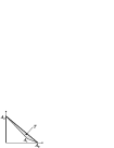
Figure 2.

We say that a distribution of signs $\epsilon$ is compatible with a polynomial $Q=\sum c_{i,j}x^{i}y^{j}\in\mathbf{R}[x,y]$ if $\mbox{{\rm sign}}(c_{i,j})=\epsilon(i,j)$.

Proposition 6.4.

With the above notations, let $P_{0}\in\mathbf{R}[x,y]$ be a semi-quasi-homogeneous polynomial defining a plane curve singularity $(C,0)$. If the peripheral roots of $P^{\Gamma}$ are all different and of the same sign, then there are two Harnack distribution of signs, $\epsilon_{1}$ and $\epsilon_{2}$, which are compatible with $P^{\Gamma}$. Let $\omega$ be as in Lemma 6.3. Then the polynomial

$$P_{t}=\sum_{(i,j)\in\Delta^{-}\cap\mathbf{Z}^{2}}\epsilon_{k}(i,j)t^{\omega(i,j)}x^{i}y^{j}+P_{0},$$

defines a Harnack smoothing of $(C,0)$, for $k=1,2$.

Proof. We keep Notations 5.2. We suppose without loss of generality that the peripheral roots of $P^{\Gamma}$ are all positive. Then the signs of the coefficients corresponding to consecutive terms in the edge $\Gamma$ are always different. By a simple observation on the set of Harnack distribution of signs it follows that there exists precisely two different Harnack distribution of signs $\epsilon,\epsilon^{\prime}$ which are compatible with $P^{\Gamma}$ (see Definition 4.7). Since $P^{\Gamma}(x,y)=P^{\Gamma}\circ\rho_{\Gamma}(x,y)$ by definition of $\rho_{\Gamma}$ (see Section 2) the distributions of signs $\epsilon$ and $\epsilon^{\prime}$ are related by $\epsilon^{\prime}=\epsilon\circ\rho_{\Gamma}$.

We use notations 3.2. Let $\omega:\Delta\rightarrow\mathbf{R}_{\geq 0}$ be a piece-wise affine convex function satisfying the statement of Lemma 6.3. By Lemma 6.3 the chart of $P^{\hat{T}}_{{1}}$ is transformed by a translation and a $SL(2,\mathbf{Z})$-transformation to the chart of a polynomial with Newton polygon with vertices $(0,0)$, $(0,1)$ and $(e,0)$, i.e., to the chart of the graph of a polynomial of one variable with $e$ different positive real roots . The topology of this chart is determined by the sign of the term corresponding to $(0,1)$. Let ${\omega}^{\prime}:\Delta\rightarrow\mathbf{R}$ be a convex piece-wise affine function determined by its integral values on $\Delta\cap\mathbf{Z}^{2}$. We can assume that $\omega^{\prime}$ induces a primitive triangulation of $T$ and of $\Delta\setminus\mbox{\rm int}T$ the functions $\omega$ and ${\omega}^{\prime}$ define the same primitive triangulation (by translating $\omega$ we can assume that $\omega_{|T}=\alpha>0$, then define $\omega^{\prime}$ as $\omega^{\prime}=\omega$ on $\Delta\setminus T$ and $\omega^{\prime}_{|A_{0}A_{2}}$ be strictly convex piece wise-linear and positive).

The topology of the chart of $P^{\hat{T}}_{{1}}$ coincides with the topology of the chart of the polynomial $\sum_{(i,j)\in T\cap\mathbf{Z}^{2}}\epsilon_{k}(i,j)t^{\tilde{\omega}(i,j)}x^{i}y^{j}$. Notice that the patchworking of $P_{t}$ is combinatorial for all triangles $T^{\prime}$ of the subdivision with the possible exception of $T$. It follows from Theorem 5.1 that the signed topological type of the smoothing $P_{t}$ coincides with that of the smoothing defined by

$$Q_{t}:=\sum_{(i,j)\in\Delta\cap\mathbf{Z}^{2}}\epsilon_{k}(i,j)t^{\tilde{\omega}(i,j)}x^{i}y^{j},$$

which is constructed by combinatorial patchworking. It follows that the polynomial $P^{\hat{\Delta}}_{{1}}$ defines a Harnack curve in the toric surface $Z(\Delta)$, by Proposition 4.8. Therefore $P_{t}$ defines then a Harnack smoothing of $(C,0)$ with $\#\mbox{{\rm int}}\Delta\cap\mathbf{Z}^{2}$ ovals and $e$ non compact components. $\Box$

6.1.2. The topological type of a Harnack smoothing

Theorem 6.1.

Let $(C,0)$ be a plane curve singularity defined by a semi-quasi-homogeneous polynomial $P_{0}\in\mathbf{R}[x,y]$ non degenerated with respect to its local Newton polygon. We denote by $\Gamma$ the compact edge of this polygon. We suppose that the peripheral roots of $P_{0}^{\Gamma}$ are all real. Let $C_{t}$ define a semi-quasi-homogeneous $M$-smoothing of $(C,0)$ such that $C_{t}$ is in maximal position with respect to the coordinate lines. If $B$ denotes a Milnor ball for $(C,0)$ then we have that:

1. The peripheral roots of $P_{0}^{\Gamma}$ are of the same sign.

2. The polynomial $P^{\hat{\Delta}}_{{1}}$ defines a Harnack curve in $Z(\Delta)$.

3. The smoothing $C_{t}$ is Harnack.

4. There is a unique topological type of triples $(\mathbf{R}{B},\mathbf{R}C_{t},B\cap(\mathbf{R}^{*})^{2})$.

5. The topological type of the smoothing $C_{t}$ is determined by $\Delta$.

Proof. We follow Notations 5.2 to describe the polynomial $P_{0}$. Since the peripheral roots of the polynomial $P_{0}^{\Gamma}$ are all real it follows that the singularity $(C,0)$ has exactly $e$ analytic branches which are all real. It follows that the smoothing $C_{t}$ has $e$ non closed components. If $C_{t}$ is $M$-smoothing there are precisely $\#(\mbox{\rm int}{\Delta}\cap\mathbf{Z}^{2})$ ovals by (7). Since the smoothing $C_{t}$ is Harnack, i.e., it is in maximal position with respect to the coordinate axis, none of these ovals cuts the coordinate axis.

We consider the curve $\tilde{C}$ defined by the polynomial $P^{\hat{\Delta}}_{{1}}$ in the real toric surface $Z(\Delta)$. By Theorem 5.1 and Remark 3.4 there are exactly $\#(\mbox{\rm int}{\Delta}\cap\mathbf{Z}^{2})$ ovals in the chart $\mbox{Ch}_{\Delta}^{*}(\tilde{C})$. These ovals, when viewed in the toric surface $Z(\Delta)$ by Proposition 2.1, do not meet any of the coordinate lines of $Z(\Delta)$. By the same argument we have that the curve $\tilde{C}$ is in maximal position with respect to the two coordinate lines $x=0$ and $y=0$ of $Z(\Delta)$, corresponding respectively to the vertical and horizontal edges of $\Delta$. It follows that the number of components of $\mathbf{R}\tilde{C}$ is $\geq 1+\#(\mbox{\rm int}{\Delta}\cap\mathbf{Z}^{2})$, which is equal to the maximal number of components, hence $\tilde{C}$ is a $M$-curve in $Z(\Delta)$.

We deduce that the non compact connected components of $\mathbf{R}\tilde{C}\cap(\mathbf{R}^{*})^{2}\subset Z(\Delta)$ glue up in one connected component of $\mathbf{R}\tilde{C}$. This component contains all the intersection points with the coordinate lines of $Z(\Delta)$, since $\tilde{C}$ is in maximal position with respect to the lines $x=0$ and $y=0$, and by assumption the peripheral roots of $P_{0}^{\Gamma}$ are all real.

By definition of maximal position with respect to two lines, there is exactly one component of the smoothing $C_{t}$ containing all the points of intersection of $C_{t}$ with the coordinate axis. We deduce the following assertion by translating this information in terms of the chart of $\tilde{C}$, using Theorem 5.1 and Proposition 2.1: there are two disjoint arcs $\mathbf{a}_{x}$ and $\mathbf{a}_{y}$ in $\mathbf{R}\tilde{C}$ containing respectively the points of intersection of $\tilde{C}$ with the toric axis $x=0$ and $y=0$, which do not contain any point in $\mathbf{R}Z(\Gamma)$ (otherwise there would be more than one non compact component of the smoothing $C_{t}$ intersecting the coordinate axis, contrary to the assumption of maximal position). It follows from this that the curve $\tilde{C}$ is in maximal position with respect to the coordinate axis in $Z(\Delta)$. Mikhalkin’s Theorem 4.1 implies the second assertion. Then the other three assertions are deduced from this by Theorem 5.1 and Proposition 4.6. $\Box$

Remark 6.5.

With the hypothesis and notations of Theorem 6.1, we have that the connected components $\Omega_{i,j}$, for $(i,j)\in\Delta\cap\mathbf{Z}^{2}$, of chart $\mbox{Ch}_{\Delta}^{*}(\tilde{C})$, are described by Proposition 4.6. If the peripheral roots of $P_{0}^{\Gamma}$ are positive, up to replacing $P^{\Delta}_{t}$ by $P^{\Delta}_{t}\circ\rho_{\Gamma}$, one can always have that $\Omega_{0,n}\subset\mathbf{R}^{2}_{0,0}$ and then:

(11) $$\Omega_{r,s}\subset\mathbf{R}^{2}_{n+s,r},\quad\forall(r,s)\in\Delta\cap\mathbf{Z}^{2}.$$

Otherwise, we have that:

(12) $$\Omega_{r,s}\subset\rho_{\Gamma}(\mathbf{R}^{2}_{n+s,r}),\quad\forall(r,s)\in\Delta\cap\mathbf{Z}^{2}.$$

Compare in Figure 3 the position of $\Omega_{0,4}$ in (A) and (B).

Definition 6.6.

If (11) holds then we say that the signed topological type of the smoothing $C_{t}$ (or of the chart of $P_{\Delta}$), is normalized (cf. Definition 5.1).

As an immediate corollary of Theorem 6.1 we deduce that:

Proposition 6.7.

There are two signed topological types of sqh-$M$-smoothings of $(C,0)$ in maximal position with respect to the coordinate axis. These types are related by the orthogonal symmetry $\rho_{\Gamma}$ and only one of them is normalized.

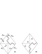
Figure 3. Charts of Harnack smoothings of $y^{4}-x^{3}=0$. The signed topological type in (A) is normalized

One of the aims of this paper is to study to which extent Theorem 6.1 admits a valid formulation in the class of real plane branch singularities. In general the singularities of this class are degenerated with respect to their local Newton polygon, in particular we cannot apply Viro’s method to those cases. Classically smoothing of this type of singularities is constructed using the blow up construction. We present in the following sections an alternative method which applies Viro method at a sequence of certain infinitely near points.

7. A reminder on toric resolutions of real plane branches

We recall the construction of an embedded resolution of singularities of a real plane branch by a sequence of local toric modifications. For details see [A’C-Ok] and [GP2]. See [Od], [Fu] for more on toric geometry and [Ok1], [Ok2], [L-Ok] and [G-T] and for more on toric geometry and plane curve singularities.

A germ $(C,0)$ of real plane curve, defined by $F=0$ for $F\in\mathbf{R}[x,y]$, defines a real plane branch if it is analytically irreducible in $(\mathbf{C}^{2},0)$ and if it admits a real Newton Puiseux parametrization (normalization map):

(13) $$\left\{\begin{array}[]{lcl}x(t)&=&t^{e_{0}},\\ y(t)&=&\sum_{i}\eta_{i}t^{i},\quad\mbox{ with }\eta_{i}\in\mathbf{R}.\end{array}\right.$$

If the coordinate line $x=0$ is not tangent to $(C,0)$ then $e_{0}=\mbox{ord}_{t}(x(t))$ is the multiplicity of $(C,0)$. By (13) and a suitable change of coordinates, we have that $C$ has an equation $F=0$, with

(14) $$F=(y^{n_{1}}-x^{m_{1}})^{e_{1}}+\cdots,$$

such that $\mbox{\rm gcd }(n_{1},m_{1})=1$, the integer $e_{0}:=e_{1}n_{1}$ is the intersection multiplicity with the line, $x=0$, and the terms which are not written have exponents $(i,j)$ such that $in_{1}+jm_{1}>n_{1}m_{1}e_{1}$, i.e., they lie above the compact edge

$$\Gamma_{1}:=[(0,n_{1}e_{1}),(m_{1}e_{1},0)]$$

of the local Newton polygon of $F$.

The vector $\vec{p}_{1}=(n_{1},m_{1})$ is orthogonal to $\Gamma_{1}$ and defines a subdivision of the positive quadrant $\mathbf{R}^{2}_{\geq 0}$, which is obtained by adding the ray $\vec{p}_{1}\mathbf{R}_{\geq 0}$. The quadrant $\mathbf{R}^{2}_{\geq 0}$ is subdivided in two cones, $\tau_{i}:=\vec{e}_{i}\mathbf{R}_{\geq 0}+\vec{p}_{1}\mathbf{R}_{\geq 0}$, for $i=1,2$ and $\vec{e}_{1},\vec{e}_{2}$ the canonical basis of $\mathbf{Z}^{2}$. We define the minimal regular subdivision $\Sigma_{1}$ of $\mathbf{R}^{2}_{\geq 0}$ which contains the ray $\vec{p}_{1}\mathbf{R}_{\geq 0}$ by adding the rays defined by those integral vectors in $\mathbf{R}^{2}_{>0}$, which belong to the boundary of the convex hull of the sets $(\tau_{i}\cap\mathbf{Z}^{2})\backslash\{0\}$, for $i=1,2$. We denote by $\sigma_{1}$ the unique cone of $\Sigma_{1}$ of the form, $\sigma_{1}:=\vec{p}_{1}\mathbf{R}_{\geq 0}+\vec{q}_{1}\mathbf{R}_{\geq 0}$ where $\vec{q}_{1}=(c_{1},d_{1})$ satisfies that:

(15) $$c_{1}m_{1}-d_{1}n_{1}=1.$$

See an example in Figure 4.

Figure 4. The subdivision $\Sigma_{1}$ associated to $F$ in Example 7.1

By convenience we denote $\mathbf{C}^{2}$ by $Z_{1}$. We define in the sequel a sequence of proper birational maps $\Pi_{j}:Z_{j+1}\rightarrow Z_{j}$, for $j=1,\dots,g$ such that the composition $\Pi_{g}\circ\dots\circ\Pi_{1}$ is an embedded resolution of the germ $(C,0)$, i.e., the pull back of the germ $(C,0)$ by $\Pi_{g}\circ\dots\Pi_{1}$ is a normal crossing divisor in the smooth surface $Z_{g+1}$.

In order to describe these maps we denote the coordinates $(x,y)$ by $(x_{1},y_{1})$ and the origin $0\in\mathbf{C}^{2}=\mathbf{Z}_{1}$ by $o_{1}$. We also denote $F$ by $F^{(1)}$ and $C$ by $C^{(1)}$. The subdivision $\Sigma_{1}$ defines a proper birational map $\Pi_{1}:Z_{2}\rightarrow Z_{1}$, which is obtained by gluing maps $\mathbf{C}^{2}(\sigma)\rightarrow\mathbf{C}^{2}$, where $\sigma$ runs through the set of two dimensional cones in $\Sigma_{1}$. For instance, the map $\pi_{1}:\mathbf{C}^{2}(\sigma_{1})\rightarrow\mathbf{C}^{2}$ is defined by

(16) $$\begin{array}[]{lcl}x_{1}&=&u_{2}^{c_{1}}x_{2}^{n_{1}},\\ y_{1}&=&u_{2}^{d_{1}}x_{2}^{m_{1}},\end{array}$$

where $u_{2},x_{2}$ are canonical coordinates for the affine space $\mathbf{C}^{2}(\sigma_{1})$.

It should be noticed that the map $\Pi_{1}$ is a composition of point blow-ups, as many as rays added in $\Sigma_{1}$ to subdivide $\mathbf{R}^{2}_{\geq 0}$. Each ray $\vec{a}\mathbf{R}_{\geq 0}\in\Sigma_{1}$ corresponds bijectively to a projective line $\mathbf{C}P^{1}$, embedded as an irreducible component of the exceptional divisor $\Pi_{1}^{-1}(0)$. We denote by $E_{2}\subset Z_{2}$ the exceptional divisor defined by $x_{2}=0$ in the chart $\mathbf{C}^{2}(\sigma_{1})$, the other exceptional divisor in this chart being defined by $u_{2}=0$. Notice that the point at the infinity of the line $x_{2}=0$, for instance, is the origin of the chart $\mathbf{C}^{2}(\sigma_{1}^{\prime})$, where $\sigma_{1}^{\prime}\in\Sigma_{1}$ is the two dimensional cone adjacent to $\sigma_{1}$ along the ray $\vec{p}_{1}\mathbf{R}_{\geq 0}$.

We have that $\Pi_{1}^{*}(C^{(1)})$ defines a Cartier divisor on $Z_{2}$. For instance, on $\mathbf{C}^{2}(\sigma_{1})$ it is defined by $F\circ\pi_{1}=0$. The term $F\circ\pi_{1}=0$ decomposes as:

(17) $$F^{(1)}\circ\pi_{1}=\mbox{\rm Exc}(F^{(1)},\pi_{1})\bar{F}^{(2)}(x_{2},u_{2}),\mbox{ where }\bar{F}^{(2)}(0,0)\neq 0,$$

and

$$\mbox{\rm Exc}(F^{(1)},\pi_{1}):=y_{1}^{e_{0}}\circ\pi_{1}.$$

The polynomial $\bar{F}^{(2)}(x_{2},u_{2})$ defines the strict transform $C^{(2)}$ of $C^{(1)}$, i.e., the closure of the pre-image by $\pi_{1}^{-1}$ of the punctured curve $C^{(1)}\setminus\{0\}$ on the chart $\mathbf{C}^{2}(\sigma_{1})$. The function $\mbox{\rm Exc}(F^{(1)},\pi_{1})$ defines the exceptional divisor of $\Pi_{1}^{*}(C^{(1)})$ on this chart.

We analyze the intersection of the strict transform with the exceptional divisor on the chart $\mathbf{C}^{2}(\sigma_{1})$: using (14) we find that $\bar{F}^{(2)}(x_{2},0)=1$ and

$$\bar{F}^{(2)}(0,u_{2})=(1-u_{2}^{c_{1}m_{1}-d_{1}n_{1}})^{e_{1}}\stackrel{{\scriptstyle\mbox{ (\ref{ave-i})}}}{{=}}(1-u_{2})^{e_{1}}.$$

By a similar argument on the other charts it follows that $E_{2}$ is the only exceptional divisor of $\Pi_{1}$ which intersects the strict transform $C^{(2)}$ of $C$, precisely at the point $o_{2}$ of the chart $\mathbf{C}^{2}(\sigma_{1})$ with coordinates $x_{2}=0$ and $u_{2}=1$, with intersection multiplicity equal to $e_{1}$. If $e_{1}=1$ then the strict transform is smooth at $o_{2}$ and the intersection with the exceptional divisor $x_{2}=0$ is transversal, hence the divisor $\Pi_{1}^{*}(C)$ has smooth components which intersect transversally. In this case, the map $\Pi_{1}$ is an embedded resolution of the germ $(C,0)$ by definition.

We define a pair of real coordinates $(x_{2},y_{2})$ at the point $o_{2}$, where

(18) $$\xi_{2}y_{2}=1-u_{2}+x_{2}R_{2}(x_{2},u_{2})\mbox{ for some }\xi_{2}\in\mathbf{R}^{*}\mbox{ and }R_{2}\in\mathbf{R}[x_{2},u_{2}],$$

such that $C^{(2)}$ is defined by a polynomial, which we call the strict transform function, of the form:

(19) $$F^{(2)}(x_{2},y_{2})=(y_{2}^{n_{2}}-x_{2}^{m_{2}})^{e_{2}}+\cdots,$$

where $\mbox{\rm gcd}(n_{2},m_{2})=1$, $e_{1}=e_{2}n_{2}$ and the terms which are not written have exponents $(i,j)$ such that $in_{2}+jm_{2}>n_{2}m_{2}e_{1}$, i.e., they lie above the compact edge $\Gamma_{2}$ of the (local) Newton polygon of $F^{(2)}(x_{2},y_{2})$. The result of substituting in $F^{(2)}(x_{2},y_{2})$, the term $y_{2}$ by using (18), is equal to $\bar{F}^{(2)}(x_{2},u_{2})$.

We can iterate this procedure defining for $j>2$ a sequence of toric maps $\Pi_{j-1}:Z_{j}\rightarrow Z_{j-1}$, which are described by replacing the index $1$ by $j-1$ and the index $2$ by $j$ above. In particular, when we refer to a Formula, like (15) at level $j$, we mean after making this replacement.

We denote by $\mbox{\rm Exc}(F^{(1)},\pi_{1}\circ\cdots\circ\pi_{j})$ the exceptional function defining the exceptional divisor of $(\Pi_{1}\circ\cdots\circ\Pi_{j})^{*}(C)$ on the chart $\mathbf{C}^{2}(\sigma_{j})\subset Z_{j}$. We have that

(20) $$\mbox{\rm Exc}(F^{(1)},\pi_{1}\circ\cdots\circ\pi_{j})=(y_{1}^{e_{0}}\circ\pi_{1}\circ\cdots\circ\pi_{j})\cdots(y_{j}^{e_{j-1}}\circ\pi_{j}).$$

Since by construction we have that $e_{j}|e_{j-1}|\cdots|e_{1}|e_{0}$ (for $|$ denoting divides), at some step we reach a first integer $g$ such that $e_{g}=1$ and then the process stops. The composition of blow ups $\Pi_{g}\circ\dots\circ\Pi_{1}$ is an embedded resolution of the germ $(C,0)$. It is minimal, in the number of exceptional divisors required, if one of the coordinate axis $x_{1}=0$ or $y_{1}=0$ is not tangent to $(C,0)$, in particular if $e_{0}$ is the multiplicity of $(C,0)$ (see [A’C-Ok]).

If $x_{1}=0$ is not tangent to $C$ then the sequence of pairs $\{(n_{j},m_{j})\}_{j=1}^{g}$ classifies the embedded topological type of the pair $(C,0)\subset(\mathbf{C}^{2},0)$. This is because the $\{(n_{j},m_{j})\}_{j=1}^{g}$ determine and are determined by the classical characteristic pairs of a plane branch (see [A’C-Ok] and [Ok1]).

Example 7.1.

The embedded resolution of the real plane branch singularity $(C,0)$ defined by $F=(y_{1}^{2}-x_{1}^{3})^{3}-x_{1}^{10}=0$ is as follows.

The morphism $\pi_{1}$ of the toric resolution is defined by

$$\begin{array}[]{lcl}x_{1}&=&u_{2}^{1}x_{2}^{2},\\ y_{1}&=&u_{2}^{1}x_{2}^{3}.\end{array}$$

Let $z_{1}:=y_{1}^{2}-x_{1}^{3}$, then we have $z_{1}\circ\pi_{1}=u_{2}^{2}x_{2}^{6}(1-u_{2})=u_{2}^{2}x_{2}^{6}y_{2}$, where $y_{2}:=1-u_{2}$ defines the strict transform function of $z_{1}$, and together with $x_{2}$ defines local coordinates at the point of intersection $o_{2}$ with the exceptional divisor $x_{2}=0$.

For $F$ we find that:

$$\begin{array}[]{lcl}F\circ\pi_{1}&=&u_{2}^{6}x_{2}^{18}\left((1-u_{2})^{3}-u_{2}^{4}x_{2}^{2}\right).\end{array}$$

Hence $\mbox{\rm Exc}(F,\pi_{1}):=y_{1}^{6}\circ\pi_{1}=u_{2}^{6}x_{2}^{18}$ is the exceptional function associated to $F$, and

$$F^{(2)}=y_{2}^{3}-(1-y_{2})^{4}x_{2}^{2}$$

is the strict transform function.

Notation 7.2.

For $j=1,\dots,g$:

1. Let $\Gamma_{j}=[(m_{j}e_{j},0),(0,n_{j}e_{j})]$, be the unique compact edge of the local Newton polygon of $F^{(j)}(x_{j},y_{j})$ (see (19) at level $j$).

2. Let $\Delta_{j}$ the Newton diagram of $F^{(j)}(x_{j},y_{j})$. We denote by $\Delta_{j}^{-}$ the set $\Delta_{j}^{-}=\Delta_{j}\setminus\Gamma_{j}$.

3. Let $\Xi_{j}=[(0,0),(0,n_{j}e_{j})]$ be the edge of $\Delta_{j}$ which is the intersection of $\Delta_{j}$ with the vertical axis.

4. Let $\omega_{j}:\Delta_{j}\cap\mathbf{Z}^{2}\rightarrow\mathbf{Z}$ be defined by

   (21) $$\omega_{j}(r,s)=e_{j}(e_{j}n_{j}m_{j}-rn_{j}-sm_{j})$$

Notice that (21) is defined analogously as (8).

Figure 5. The Newton diagrams in Notation 7.2

Proposition 7.3.

The following formula for the Milnor number of $(C,0)$ at the origin is deduced in [GP2].

(22) $$\mu(C)_{0}=2\sum_{j=1}^{g}\#(\mbox{{\rm int}}\Delta_{j}\cap\mathbf{Z}^{2})+e_{j}-1.$$

7.1. A set of polynomials defined from the embedded resolution

We associate in this section some polynomials to the elements in $\Delta_{j}^{-}\cap\mathbf{Z}^{2}$. From these polynomials we define a class of deformations which we will study in the following sections.

Lemma 7.4.

If $(r,s)\in\mathbf{Z}^{2}_{\geq 0}$ with $s<e_{j-1}$ there exist $M_{j}(r,s)\in\mathbf{R}[x_{1},y_{1}]$ and integers $k_{2}>0,\dots,k_{j}>0$ such that:

(23) $$\mbox{\rm Exc}(F,\pi_{1}\circ\cdots\circ\pi_{j-1})\,u_{2}^{k_{2}}\cdots u_{j}^{k_{j}}\,x_{j}^{r}\,y_{j}^{s}=M_{j}(r,s)\circ\pi_{1}\circ\cdots\circ\pi_{j-1}.$$

To avoid cumbersome notations we denote simply by $u_{i}$ the term $u_{i}\circ\pi_{i}\circ\cdots\circ\pi_{j-1}$, whenever $j>i$ is clear form the context. For instance we have done this in Formula (23) above. In particular, by (18) at level $\leq j$, the restriction of the function $u_{i}$ to $x_{j}=0$ is equal to:

(24) $$u_{i}=\left\{\begin{array}[]{lcl}1&\mbox{ if }&i<j,\\ 1-\xi_{j}y_{j}&\mbox{ if }&i=j\end{array}\right.$$

Remark 7.5.

The integers $k_{2},\dots,k_{j}$ depend on $(r,s)$ and on the singular type of the branch $(C,0)$. They can be determined algorithmically, and are unique up to certain conditions on the polynomials $M_{j}(r,s)$. The polynomials $M_{j}(r,s)$ are constructed as monomials in $x_{1},y_{1}$ and some Weierstrass polynomials defining curvettes at certain irreducible exceptional divisors of the embedded resolution of $(C,0)$ (see [GP2]). For more details on the construction of these curves and their applications see [PP], [G-T], [Z2] and [A-M].

Example 7.6.

The following table indicates the terms $M_{2}(r,s)$ for $(r,s)\in\Delta_{2}$ corresponding to Example 7.1. The symbol $z_{1}$ denotes the first approximate root $y_{1}^{2}-x_{1}^{3}$.

$(r,s)$	$(0,0)$	$(0,1)$	$(0,2)$	$(1,1)$	$(1,0)$
$M_{2}(r,s)$	$x_{1}^{9}$	$x_{1}^{6}z_{1}$	$x_{1}^{3}z_{1}^{2}$	$x_{1}^{5}y_{1}z_{1}$	$x_{1}^{8}y_{1}$

For instance, we have that $M_{2}(1,1)=x_{1}^{5}y_{1}z_{1}$, since $x_{1}^{5}y_{1}z_{1}\circ\pi_{1}=\mbox{\rm Exc}(F^{(1)},\pi_{1})u_{2}^{2}x_{2}y_{2}$, where $\mbox{\rm Exc}(F^{(1)},\pi_{1})=u_{2}^{6}x_{2}^{18}$ by Example 7.1.

8. Multi-semi-quasi-homogeneous smoothings of a real plane branch

In this Section we introduce a class of deformations of a plane branch $(C,0)$, called multi-semi-quasi-homogeneous (msqh) deformations and we describe their basic properties.

We suppose that $(C,0)$ is a plane branch defined by an equation, $F(x,y)=0$, such that its embedded resolution consists of $g$ toric maps (see Section 7 and Notation 7.2). Consider the following algebraic expressions in terms of the polynomials of Lemma 7.4 as a sequence of deformations of the polynomial $F(x_{1},y_{1})$ defining $C$. We denote by $M_{1}(r,s)$ the monomial $x_{1}^{r}y_{1}^{s}$ and ${\underline{t}}_{j}$ will denote $t_{j},\dots,t_{g}$ for any $1\leq j\leq g$.

(25) $$\left\{\begin{array}[]{ccccccl}P_{{\underline{t}}_{g}}&:=&F&+&\displaystyle{\sum_{(r,s)\in\Delta_{g}^{-}\cap\mathbf{Z}^{2}}}\,A_{r,s}^{(g)}&t_{g}^{\omega_{g}(r,s)}&M_{g}(r,s)\\ P_{{\underline{t}}_{g-1}}&:=&P_{{\underline{t}}_{g}}&+&\displaystyle{\sum_{(r,s)\in\Delta_{g-1}^{-}\cap\mathbf{Z}^{2}}}\,A_{r,s}^{(g-1)}&t_{g-1}^{\omega_{g-1}(r,s)}\,{}_{0\leq s<e_{g-1}}^{0\leq r}\alpha_{g-1,r,s}(\lambda_{g-1})&M_{g-1}(r,s)\\ \dots&\dots&\dots&\dots&\dots&\dots&\dots\\ P_{{\underline{t}}_{1}}&:=&P_{{\underline{t}}_{2}}&+&\displaystyle{\sum_{(r,s)\in\Delta_{1}^{-}\cap\mathbf{Z}^{2}}}\,A_{r,s}^{(1)}&t_{1}^{\omega_{1}(r,s)}&M_{1}(r,s).\end{array}\right.$$

The terms $A_{r,s}^{(j)}$ are some real constants while the $t_{j}$ are real parameters, for $j=1,\dots,g$. For technical reasons we will suppose that $A_{0,0}^{(j)}\neq 0$ for $j=1,\dots,g$ (we need this assumption in Proposition 8.3 and 8.5). The choice of the notation ${\underline{t}}_{j}=(t_{j},\dots,t_{g})$ in the deformation $P_{{\underline{t}}_{j}}$ is related to the fact that the terms $M_{l}(r,s)$ appearing in the expansion of $P_{{\underline{t}}_{j}}$ are expressed in terms of the monomial $x_{l}^{r}y_{l}^{s}$ at the local coordinates of the level $l$ of the embedded resolution of $(C,0)$, for $j\leq l\leq g$. Notice that the polynomial $P_{{\underline{t}}_{1}}$ determines any of the terms $P_{{\underline{t}}_{j}}$ for $1<j\leq g$, by substituting $t_{1}=\dots=t_{j-1}=0$ in $P_{{\underline{t}}_{1}}$. Occasionally, we abuse of notation by denoting $F$ by $P_{{\underline{t}}_{g+1}}$.

Definition 8.1.

A multi-semi-quasi-homogeneous (msqh) deformation of the plane branch $(C,0)$ is a family $C_{{\underline{t}}_{1}}$ defined by, $P_{{\underline{t}}_{1}}=0$ where $P_{{\underline{t}}_{1}}$ is of the form (25), in a Milnor ball of $(C,0)$. We say that $C_{{\underline{t}}_{1}}$ is a msqh-smoothing of $(C,0)$ if the curve $C_{{\underline{t}}_{1}}$ is smooth and transversal to the boundary of a Milnor ball for $0<t_{1}\ll\cdots\ll t_{g}\ll 1$.

Notation 8.2.

We denote by $C_{{\underline{t}}_{l}}$, or by $C_{{\underline{t}}_{l}}^{(1)}$, the deformation of $(C,0)$ defined by $P_{{\underline{t}}_{l}}$ in a Milnor ball of $(C,0)$, for $0<t_{l}\ll\cdots\ll t_{g}\ll 1$ and $l=1,\dots,g$.

We denote by $C_{{\underline{t}}_{l}}^{(j)}\subset Z_{j}$ the strict transform of $C_{{\underline{t}}_{l}}$ by the composition of toric maps $\Pi_{j-1}\circ\cdots\circ\Pi_{1}$ and by $P_{{\underline{t}}_{l}}^{(j)}(x_{j},y_{j})$ (resp. by $\bar{P}_{{\underline{t}}_{l}}^{(j)}(x_{j},u_{j})$) the polynomial defining $C_{{\underline{t}}_{l}}^{(j)}$ in the coordinates $(x_{j},y_{j})$ (resp. $(x_{j},u_{j})$), for $2\leq j\leq l\leq g$.

These notations are analogous to those used for $C$ in Section 7, see (17). In particular, we have that the result of substituting in $P_{{\underline{t}}_{j}}^{(j)}(x_{j},y_{j})$, the term $y_{j}$, by using Formula (18) at level $j$, is $\bar{P}_{{\underline{t}}_{l}}^{(j)}(x_{j},u_{j})$.

Proposition 8.3.

([GP2])

1. If $1\leq j<l\leq g$ the curves $C_{{\underline{t}}_{l}}^{(j)}$ and $C^{(j)}$ meet the exceptional divisor of $\Pi_{j-1}\circ\cdots\circ\Pi_{1}$ only at the point $o_{j}\in E_{j}$ and with the same intersection multiplicity $e_{j-1}$.

2. If $1<j\leq g$ the curves $C_{{\underline{t}}_{j}}^{(j)}$ meet the exceptional divisor of $\Pi_{j-1}\circ\cdots\circ\Pi_{1}$ only at $e_{j}$ points of $E_{j}$, counted with multiplicity.

Remark 8.4.

([GP2])

1. If $1\leq j<l\leq g$ the local Newton polygon of $P_{{\underline{t}}_{l}}^{(j)}(x_{j},y_{j})$ and of $F^{(j)}(x_{j},y_{j})$ coincide.

2. If $1<j\leq g$ then $\Xi_{j}$ is a face of the Newton polygons of $\bar{P}_{{\underline{t}}_{j}}^{(j)}(x_{j},u_{j})$ and of $P_{{\underline{t}}_{j}}^{(j)}(x_{j},y_{j})$ corresponding to those terms which are not divisible by $x_{j}$ (see Notations 7.2).

Proposition 8.5.

(see [GP2]) If $1<j\leq g$ then we have that:

1. The symbolic restriction of $P^{(j)}_{{\underline{t}}_{j+1}}(x_{j},y_{j})$ to the edge $\Gamma_{j}$ of its local Newton polygon is of the form:

   $$\alpha_{j}\prod_{s=1}^{e_{j}}\left(y_{j}^{n_{j}}-(1+\gamma_{s}^{(j)}t_{j+1}^{e_{j+1}m_{j+1}})x_{j}^{m_{j}}\right),$$

   where $\alpha_{j},\gamma_{s}^{(j)}\in\mathbf{C}\setminus\{0\}$, for $s=1,\dots,e_{j}$.

2. The points of intersection of $E_{j+1}$ with $C_{{\underline{t}}_{j+1}}^{(j+1)}$ are those with coordinates $x_{j+1}=0$ and

   (26) $$u_{j+1}=(1+\gamma_{s}^{(j)}t_{j+1}^{e_{j+1}m_{j+1}})^{-1},\mbox{ for }s=1,\dots,e_{j}.$$

Remark 8.6.

It follows from Proposition 8.5 that those peripheral roots of $P^{(j)}_{{\underline{t}}_{j+1}}(x_{j},y_{j})$, which are real, are also positive for $0<t_{j+1}\ll 1$.

When we say that $C_{{\underline{t}}_{l}}^{(j)}$ defines a deformation with parameter $t_{l}$, we mean for $t_{l+1},\dots t_{g}$ fixed. Proposition 8.7 motivates our choice of terminology in this section.

Proposition 8.7.

$C_{{\underline{t}}_{j}}^{(j)}$ is a sqh-deformation with parameter $t_{j}$ of the singularity $(C_{{\underline{t}}_{j+1}}^{(j)},o_{j})$ for $1\leq j\leq g$.

Proof. By Proposition 8.3 the curves $C_{{\underline{t}}_{j+1}}^{(j)}$ and $C_{{\underline{t}}_{j}}^{(j)}$ intersect only the irreducible component $E_{j}$ of the exceptional divisor of $\Pi_{j-1}\circ\dots\circ\Pi_{1}$. By the construction of the toric resolution this intersection is contained in the chart $\mathbf{C}^{2}(\sigma_{j-1})\subset Z_{j}$. By Lemma 7.4 and the definitions in Formula (25), if $C_{{\underline{t}}_{j+1}}^{(j)}$ is defined on the chart $\mathbf{C}^{2}(\sigma_{j-1})$ by $P_{{\underline{t}}_{j+1}}^{(j)}(x_{j},y_{j})$ then $C_{{\underline{t}}_{j}}^{(j)}$ is defined by:

$$P_{{\underline{t}}_{j}}^{(j)}(x_{j},y_{j})=\sum_{(r,s)\in\Delta_{j}^{-}\cap\mathbf{Z}^{2}}A_{r,s}^{(j)}\,t_{j}^{\omega_{j}(r,s)}\underline{u}^{\underline{k}(r,s)}\,x_{j}^{r}\,y_{j}^{s}+P_{{\underline{t}}_{j+1}}^{(j)}(x_{j},y_{j}),$$

where for each $(r,s)$ the term $\underline{u}^{\underline{k}(r,s)}$ denotes the term $u_{1}^{k_{1}}\cdots u_{j}^{k_{j}}$ of (23). The elements $u_{1},\dots,u_{j}$, expanded in terms of $x_{j},y_{j}$, have constant term equal to one by (24). It follows from this that the local Newton polygon of $P_{{\underline{t}}_{j}}^{(j)}(x_{j},y_{j})$, with respect to the variables $x_{j}$, $y_{j}$ and $t_{j}$, has only one compact face of dimension two, which is equal to the graph of $\omega_{j}$ on the Newton diagram $\Delta_{j}$. $\Box$

Notice that the polynomial, $(P_{{\underline{t}}_{j}}^{(j)})^{\hat{\Delta}_{j}}_{t_{j}=1}$, defining the chart of the sqh-smoothing in Proposition 8.7 does not depend on $t_{j}$ (see Notation 3.2). We have that:

(27) $$(P_{{\underline{t}}_{j}}^{(j)})^{\hat{\Delta}_{j}}_{t_{j}=1}=\sum_{(r,s)\in\Delta_{j}^{-}\cap\mathbf{Z}^{2}}A_{r,s}^{(j)}\,x_{j}^{r}\,y_{j}^{s}+(P_{{\underline{t}}_{j+1}}^{(j)})^{\Gamma_{j}},$$

where $(P_{{\underline{t}}_{j+1}}^{(j)})^{\Gamma_{j}}$ is described by Proposition 8.5.

Definition 8.8.

The msqh-deformation $C_{{\underline{t}}_{1}}$ is real non degenerated if the polynomials $(P_{{\underline{t}}_{j}}^{(j)})^{\hat{\Delta}_{j}}_{t_{j}=1}$ in (27) are real non degenerated with respect to the polygon $\Delta_{j}$, for $j=0,\dots,g-1$ (see Notations 3.2).

Proposition 8.9.

If the msqh-deformation $C_{{\underline{t}}_{1}}$ is real non degenerated then $C_{{\underline{t}}_{j}}^{(j)}$ is a msqh-smoothing of the singularity $(C^{(j)},o_{j})$. In particular, $C_{{\underline{t}}_{1}}$ is a msqh-smoothing of $(C,0)$.

Proof. We prove the Proposition by induction on $g$. If $g=1$ then the assertion is a consequence of Definition 5.3. Suppose $g>1$, then by the induction hypothesis $C_{{\underline{t}}_{2}}^{(2)}$ is a msqh-smoothing of $(C^{(2)},o_{2})$. By Proposition 8.5 the polynomial $P_{{\underline{t}}_{2}}(x,y)$, defining the curve $C_{{\underline{t}}_{2}}$, is non degenerated with respect to its local Newton polygon. By Definition 5.3 the deformation $C_{{\underline{t}}_{1}}$ is a sqh-smoothing of $(C_{{\underline{t}}_{2}},0)$ with parameter $t_{1}$. It follows that $C_{{\underline{t}}_{1}}$ defines then a msqh-smoothing of $(C,0)$ for $0<t_{1}\ll\cdots\ll t_{g}\ll 1$. $\Box$

8.1. Gluing the charts of msqh-smoothings

In this Section we describe the patchwork of the charts of $(P_{{\underline{t}}_{j}}^{(j)})^{\hat{\Delta}_{j}}_{t_{j}=1}$ and of $P_{{\underline{t}}_{j+1}}^{(j)}$ at the level $j$ of the toric resolution, under some geometrical assumptions. We begin by some Lemmas for sqh-smoothings.

Lemma 8.10.

Let us consider a semi-quasi-homogeneous smoothing $C_{t}$ defined by $P_{t}(x,y)=0$ of $(C,0)$ (see Notations 5.2). Set $\Lambda_{0}$ for the Newton polygon of $P_{0}$. Suppose that the following statements hold:

1. The chart $\mbox{\rm Ch}_{\Lambda_{0}/\sim}(P_{0})$ is in maximal position with respect to $\tilde{\Gamma}/\sim$.

2. The chart $\mbox{\rm Ch}_{\Delta/\sim}(P^{\hat{\Delta}}_{{1}})$ is in maximal position with respect to $\tilde{\Gamma}/\sim$.

3. The order of the peripheral roots of $P^{\Gamma}$ coincide when viewed in suitable arcs of the charts $\mbox{\rm Ch}_{\Lambda_{0}/\sim}(P_{0})$ and $\mbox{\rm Ch}_{\Delta/\sim}(P^{\hat{\Delta}}_{{1}})$.

We label the peripheral roots $\alpha_{1},\dots,\alpha_{e}\in\tilde{\Gamma}/\sim$ of $P^{\Gamma}$ with the order induced by the arcs the charts in (i) and (ii). We denote by $\mathbf{a}_{{{k}}}{(j,j+1)}$ the arc of the chart in (k), for $k={{i,ii}}$, which joins the peripheral roots $\alpha_{j}$ and $\alpha_{j+1}$, for $j=1,\dots,e-1$. Then exactly one of this two statements is verified:

1. In the patchwork of the charts of $P^{\hat{\Delta}}_{{1}}((x,y))$ and of $P_{0}$ the arcs $\mathbf{a}_{{{i}}}{(j,j+1)}$ and $\mathbf{a}_{{{ii}}}{(j,j+1)}$ glue into an oval intersecting $\tilde{\Gamma}$, for $j=1,\dots,e-1$.

2. In the gluing of the charts of $P^{\hat{\Delta}}_{{1}}(\rho_{\Gamma}(x,y))$ and of $P_{0}$ the arcs $\mathbf{a}_{{{i}}}{(j,j+1)}$ and $\rho_{\Gamma}(\mathbf{a}_{{{ii}}}{(j,j+1)})$ glue into an oval intersecting $\tilde{\Gamma}$, for $j=1,\dots,e-1$.

Proof. If $e=1$ there is nothing to prove, hence we suppose that $e>1$. By forgetting the relation $\sim$, we obtain two symmetric copies of $\alpha_{1},\dots,\alpha_{e}$ in $\tilde{\Gamma}$, by the action of the symmetry $\rho_{\Gamma}$ (see notations of Section 2). We denote by $\mathbf{a}_{k}{(1)}$ (resp. by $\mathbf{a}_{{{k}}}{(e)}$) the arc of chart in (k), for $k=\mbox{{\rm i,ii}}$, which intersects $\mathbf{a}_{{{k}}}{(1,2)}$ at $\alpha_{1}$ (resp. $\mathbf{a}_{{{k}}}{(e-1,e)}$ at $\alpha_{e}$).

By Theorem 5.1 if the arcs $\mathbf{a}_{{{i}}}{(1,2)}$ and $\mathbf{a}_{{{ii}}}{(1,2)}$ glue up in an oval intersecting $\tilde{\Gamma}$ in the gluing of the charts of $P^{\hat{\Delta}}_{{1}}(x,y)$ and of $P_{\Lambda_{0}}$, then the assertion of the Lemma holds for $\rho=Id$, otherwise the assertion of the Lemma holds for $\rho=\rho_{\Gamma}$. $\Box$

The dotted style curve in Figure 6 represents the two possibilities for the chart of $P^{\hat{\Delta}}_{{1}}$ with good oscillation. Cases (A) and (B) correspond to assertion (a) and (b) respectively, where in this case $\rho_{\Gamma}$ is the symmetry $\rho_{\Gamma}(r,s)=(r,-s)$.

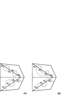
Figure 6. A represents regular intersection of charts

The following terminology is introduced, with a slightly different meaning, in [K-R-S]:

Definition 8.11.

We say that the charts of $P^{\hat{\Delta}}_{{1}}$ and of $P_{0}$, associated with the sqh-smoothing $C_{t}$, have regular intersection along $\Gamma$ if the statement (a) of Lemma 8.10 hold.

Lemma 8.12.

Suppose that in the Lemma 8.10 statement (a) holds. If in addition there exists (resp. there does not exist) a connected component of the chart $\mbox{\rm Ch}^{*}_{\Lambda_{0}}(P_{0})$ bounded by $\alpha_{1}$ and $\alpha_{e}$ then in the gluing of the charts of $P^{\hat{\Delta}}_{{1}}((x,y))$ and of $P_{0}$ the arcs $\mathbf{a}_{{{i}}}{(1)}$, $\mathbf{a}_{{{ii}}}{(1)}$, $\mathbf{a}_{{{i}}}{(e)}$ and $\mathbf{a}_{{{ii}}}{(e)}$ are contained (resp. are not contained) in an oval intersecting $\tilde{\Gamma}$.

Proof. Notice that by construction the arcs $\mathbf{a}_{{{i}}}{(1)}$ glue with $\mathbf{a}_{{{ii}}}{(1)}$ (resp. for $\mathbf{a}_{{{i}}}{(e)}$ and $\mathbf{a}_{{{ii}}}{(e)}$).

The arcs $\mathbf{a}_{{{ii}}}{(1)}$ and $\mathbf{a}_{{{ii}}}{(e)}$ are in the same connected component of the chart $\mbox{\rm Ch}_{\Delta/\sim}(P^{\hat{\Delta}}_{{1}})$ since this chart is compact and hence each connected component is an oval in particular the one which is in maximal position with respect to $\tilde{\Gamma}/\sim$.

The statement follows easily from these observations and the hypothesis. $\Box$

Figures 6 case (A) and 7 represent the two possibilities indicated in Lemma 8.12 when the chart $P^{\hat{\Delta}}_{{1}}$ has good oscillation with respect to $\tilde{\Gamma}/\sim$.

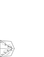
Figure 7. Regular intersection of charts

Denote by ${\Lambda}_{2}$ the Newton polygon of $P_{{\underline{t}}_{2}}(x_{1},y_{1})$. Notice that ${\Lambda}_{2}$ contains the Newton polygon of $F^{(1)}(x_{1},y_{1})$ and shares with it the common edge $\Gamma_{1}$ by Remark 8.4 (i). We denote by $\bar{\Lambda}_{2}^{(2)}$ the Newton polygon of $\bar{P}_{{\underline{t}}_{2}}^{(2)}(x_{2},u_{2})$.

Proposition 8.13.

Let $C_{{\underline{t}}_{1}}$ be a real non degenerated msqh-smoothing of $(C,0)$. If the smoothing $C_{{\underline{t}}_{2}}^{(2)}$ of $(C^{({2})},o_{2})$ is in maximal position (resp. has good oscillation) with respect to the line $E_{2}$ then in a neighborhood of $\tilde{\Gamma}_{{1}}/\sim$, the chart $\mbox{\rm Ch}_{\Lambda_{2}/\sim}(P_{{\underline{t}}_{2}}(x_{1},y_{1}))$ is in maximal position (resp. has good oscillation) with respect to $\tilde{\Gamma}_{{1}}/\sim$.

Proof. By (17) we have that:

$$P_{{\underline{t}}_{2}}\circ\pi_{{1}}=\mbox{{\rm Exc}}(P_{{\underline{t}}_{2}},\pi_{1})\cdot\bar{P}_{{\underline{t}}_{2}}^{(2)}(x_{2},u_{2}),$$

where $\mbox{{\rm Exc}}(P_{{\underline{t}}_{2}},\pi_{1})$ is a monomial in $x_{2}$ and $u_{2}$. Notice that $\bar{P}_{{\underline{t}}_{2}}^{(2)}(0,u_{2})$ is a polynomial of degree $e_{1}$ with non zero constant term by Proposition 8.3 (ii). Denote by $\phi$ the composition of the $\mbox{{\rm SL}}(2,\mathbf{Z})$ transformation corresponding to (16) with the translation induced by the exponent of the monomial $\mbox{{\rm Exc}}(P_{{\underline{t}}_{2}},\pi_{1})$. Then we have that $\phi$ is an isomorphism of triples

(28) $$\left(\bar{\Lambda}_{2}^{(2)},\Xi_{2},\mbox{\rm Ch}_{\bar{\Lambda}_{2}^{(2)}/\sim}(\bar{P}_{{\underline{t}}_{2}}^{(2)}(x_{2},u_{2}))\right)\stackrel{{\scriptstyle\phi}}{{\longrightarrow}}\left({\Lambda}_{2},\Gamma_{{1}},\mbox{\rm Ch}_{{\Lambda}_{2}/\sim}(P_{{\underline{t}}_{2}}(x_{{1}},y_{{1}}))\right).$$

In other terms $\pi_{1}$ induces an isomorphism of the toric surfaces associated to these Newton polygons which maps the one dimensional orbit associated to $\Gamma_{{1}}$ to the orbit associated to $\Xi_{2}$. More precisely, a point of the orbit of $\Gamma_{{1}}$ is defined by the vanishing of $y_{{1}}^{n_{1}}-\theta x_{{1}}^{m_{1}}$ for some $\theta\in\mathbf{C}^{*}$ and then by the computations of Section 7 it corresponds to the point of coordinates $x_{2}=0$ and $u_{2}=\theta^{-1}$, identified with the orbit associated to $\Xi_{2}$. This implies that the following assertions are equivalent:

1. In a neighborhood of the line $\tilde{\Xi}_{2}/\sim$, the chart $\mbox{\rm Ch}_{\bar{\Lambda}_{2}^{(2)}/\sim}(\bar{P}_{{\underline{t}}_{2}}^{(2)}(x_{2},u_{2}))$ is in maximal position (resp. has good oscillation) with respect to the line $\tilde{\Xi}_{2}/\sim$.

2. In a neighborhood of the line, $\tilde{\Gamma}_{{1}}/\sim$, the chart $\mbox{\rm Ch}_{{\Lambda}_{2}/\sim}(P_{{\underline{t}}_{2}}(x_{{1}},y_{{1}}))$ is in maximal position (resp. has good oscillation) with respect to $\tilde{\Gamma}_{{1}}/\sim$.

If the smoothing $C_{{\underline{t}}_{2}}^{(2)}$ is in maximal position (resp. has good oscillation) with respect to the line $E_{2}$ then there is an arc of the smoothing $\mathbf{R}C_{{\underline{t}}_{2}}^{(2)}$ which contains the points $E_{2}\cap C_{{\underline{t}}_{2}}^{(2)}$ and satisfies the geometrical hypothesis with respect to the line $E_{2}$. By Proposition 8.3 this arc does not intersect the coordinate line corresponding to $u_{2}=0$ in the chart. This implies that (a) holds and hence (b) holds. $\Box$

Lemma 8.14.

Let $C_{{\underline{t}}_{1}}$ be a real non degenerated msqh-smoothing of $(C,0)$. Suppose that the charts $\mbox{\rm Ch}^{*}_{\Delta_{1}}(P^{\hat{\Delta}_{1}}_{t_{1}=1}(x_{1},y_{1}))$ and $\mbox{\rm Ch}^{*}_{\Lambda_{2}}(P_{{\underline{t}}_{2}}(x_{1},y_{1}))$ have regular intersection along $\Gamma_{1}$ (see Definition 8.11). If the connected component of $C_{{\underline{t}}_{2}}^{(2)}$ which meets $E_{2}$ is an oval (resp. it is not an oval), then there are precisely $e_{1}$ ovals (resp. $e_{1}-1$ ovals and one non closed component) which intersect $\tilde{\Gamma}_{1}$ in the Patchwork of the charts $\mbox{\rm Ch}^{*}_{\Lambda_{2}}(P_{{\underline{t}}_{2}}^{({1})})$ and of $\mbox{\rm Ch}^{*}_{\Delta_{1}}(P^{\hat{\Delta}_{1}}_{t_{1}=1})$, which describes the smoothing $C_{{\underline{t}}_{1}}$ of $C_{{\underline{t}}_{2}}$. In addition, if the chart $\mbox{\rm Ch}_{{\Lambda}_{2}/\sim}(P_{{\underline{t}}_{2}}(x_{{1}},y_{{1}}))$ has good oscillation) with respect to $\tilde{\Gamma}_{{1}}/\sim$ and if $P^{\hat{\Delta}_{1}}_{t_{1}=1}$ defines a Harnack curve in $Z(\Delta_{1})$, then the signed topological type of the chart of $P^{\hat{\Delta}_{1}}_{t_{1}=1}$ is unique.

Proof. Notice that by hypothesis and Proposition 8.13 the smoothing $C_{{\underline{t}}_{2}}^{(2)}$ is in maximal position with respect to the line $E_{2}$. We have that the chart of $\mbox{\rm Ch}_{\Lambda_{2}/\sim}(P_{{\underline{t}}_{2}})$ is in maximal position with respect to the line $\Gamma_{1}/\sim$. We denote by $\alpha_{1},\dots\alpha_{e_{1}}$ the peripheral roots of $P_{{\underline{t}}_{2}}^{\Gamma_{1}}$, labelled with respect to the order in the charts $\mbox{\rm Ch}_{\Lambda_{2}/\sim}(P_{{\underline{t}}_{2}})$ and $\mbox{\rm Ch}_{\Delta_{1}/\sim}(P^{\hat{\Delta}_{1}}_{t_{1}=1})$. Then there exist $e_{1}-1$ ovals meeting $\tilde{\Gamma}_{1}$ in the patchwork of these charts by Lemma 8.10. In addition, if the connected component of $\mathbf{R}C_{{\underline{t}}_{2}}^{(2)}$ which meets $E_{2}$ is an oval (resp. is not an oval), then the hypothesis of Lemma 8.12 are satisfied and the conclusion follows. For the second statement by Proposition 6.7 we have that there are two possible signed topological types for $P_{\Delta}$ with prescribed symbolic restriction to the face $\Gamma_{1}$. By Lemma 8.10 only one of these two types induces regular intersection along the edge $\Gamma_{1}$. $\Box$

We call the ovals described by Lemma 8.14 mixed ovals of depth $1$. We call ovals of depth $1$, those which appear in the chart of $P^{\hat{\Delta}_{1}}_{t_{1}=1}$ (see (27)) but do not cut $\tilde{\Gamma}_{1}$. In Figure 8 we represent a mixed oval of depth one; the ball $B$ is a Milnor ball for $(C_{{\underline{t}}_{2}},0)$, the segment of the oval in small ball $B^{\prime}$ corresponds to an arc of the chart of $P^{\hat{\Delta}_{1}}_{t_{1}=1}$, while the segment of the oval in $B\setminus B^{\prime}$ corresponds to an arc of the chart $\mbox{\rm Ch}_{\Lambda_{2}/\sim}(P_{{\underline{t}}_{2}})$.

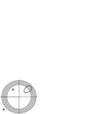
Figure 8. A mixed oval

Definition 8.15.

Let $C_{{\underline{t}}_{1}}$ be a msqh-smoothing of $(C,0)$. An oval $O$ of $C_{{\underline{t}}_{1}}$ is of depth $j$ (resp. a mixed oval of depth $j$) if there exists an oval $O_{j}$ of depth $1$ (resp. a mixed oval of depth $1$) of the smoothing $\mathbf{C}_{{\underline{t}}_{j}}^{(j)}$ of $(C^{(j)},o_{j})$ such that $E_{j}\cap O_{j}=\emptyset$ and such that $O$ arises as a slight perturbation of the oval $\Pi_{1}\circ\cdots\circ\Pi_{j-1}(O_{j})$ of $C_{{\underline{t}}_{j}}$, for $1\leq j\leq g$.

8.2. Maximal, Harnack and multi-Harnack smoothings

We introduce the following notions for a real non degenerated msqh-smoothing $C_{{\underline{t}}_{1}}$ of a real plane branch $(C,0)$. By Proposition 8.9 if $C_{{\underline{t}}_{1}}$ is a non degenerated msqh-smoothing of $(C,0)$ then $C_{{\underline{t}}_{j}}^{(j)}$ is also a non degenerated msqh-smoothing of $(C^{(j)},o_{j})$, for $1\leq j\leq g$.

Definition 8.16.

1. $C_{{\underline{t}}_{1}}$ is a $M$-smoothing if the number of ovals in a Milnor ball of $(C,0)$ is equal to $\frac{1}{2}\mu(C)_{0}$.

2. A $M$-smoothing $C_{{\underline{t}}_{1}}$ is Harnack if it has good oscillation with respect to the coordinate axis.

3. A $M$-smoothing $C_{{\underline{t}}_{1}}$ is multi-Harnack if $C_{{\underline{t}}_{j}}^{(j)}$ is a Harnack $M$-msqh-smoothing of $(C^{(j)},o_{j})$, for $1\leq j\leq g$.

In Definition 8.16 (iii) the Harnack condition is considered with respect to the coordinate lines defined by the coordinates $(x_{j},y_{j})$, see Section 7 for notations.

The following result describes inductively $M$-msqh-smoothings and Harnack msqh-smoothings of $(C,0)$ when $g>1$.

Theorem 8.1.

Let $C_{{\underline{t}}_{1}}$ be a non degenerated msqh-smoothing of the real plane branch $(C,0)$. We introduce the following conditions:

1. $C_{{\underline{t}}_{2}}^{(2)}$ is a $M$-msqh-smoothing of $(C^{(2)},o_{2})$ in maximal position with respect to the exceptional divisor $E_{2}$.

2. $C_{{\underline{t}}_{1}}$ defines a $M$-sqh-smoothing of the singularity $(C_{{\underline{t}}_{2}},0)$ with parameter $t_{1}$.

3. The charts of $P^{\hat{\Delta}_{1}}_{t_{1}=1}$ and of $P_{{\underline{t}}_{2}}$ have regular intersection along $\Gamma_{1}$.

Then, the deformation $C_{{\underline{t}}_{1}}$ is a $M$ (resp Harnack) msqh-smoothing of $(C,0)$ if and only if conditions (i), (ii) and (iii) hold (resp. and in addition $C_{{\underline{t}}_{1}}$ has good oscillation with respect to the coordinate axis).

Proof. We prove first that if conditions (i) and (ii) hold then $C_{{\underline{t}}_{1}}$ is a $M$-msqh-smoothing of $(C,0)$. The number of ovals of the msqh-smoothing $C_{{\underline{t}}_{2}}^{(2)}$ is equal to

(29) $$\frac{1}{2}\mu(C^{(2)})_{o_{2}}\stackrel{{\scriptstyle(\ref{mu-delta-j})}}{{=}}\sum_{j=2}^{g}\left(\#(\mbox{{\rm int}}\Delta_{j}\cap\mathbf{Z}^{2})+e_{j}-1\right).$$

Since $C_{{\underline{t}}_{2}}^{(2)}$ is in maximal position with respect to $E_{2}$ there is only one connected component $A$ of the smoothing $C_{{\underline{t}}_{2}}^{(2)}$ which intersect $E_{2}$ in $e_{1}$ different real points. When we apply the toric morphism $\pi_{1}$ we get a deformation $(C_{{\underline{t}}_{2}},0)$ of $(C,0)$, defined by $P_{{\underline{t}}_{2}}(x,y)$. Notice that $(C_{{\underline{t}}_{2}},0)$ is singular at $0$. By Proposition 8.5 the singularity $P_{{\underline{t}}_{2}}(x,y)=0$ is real non degenerated with respect its local Newton polygon. The image $A^{\prime}$ by $\pi_{1}$ of the component $A$ passes through the origin and is the only connected component of $\mathbf{R}C_{{\underline{t}}_{2}}$ with this property. The deformation $C_{{\underline{t}}_{2}}$ has the same number of ovals as $C_{{\underline{t}}_{2}}^{(1)}$, which are of depth $>1$.

By hypothesis (ii) we have that $C_{{\underline{t}}_{1}}$ is a $M$-sqh-smoothing of $C_{{\underline{t}}_{2}}$ with parameter $t_{1}$ hence it yields $\#(\mbox{{\rm int}}\Delta_{1}\cap\mathbf{Z}^{2})$ ovals of depth $1$. By Proposition 8.13 the chart of $P_{{\underline{t}}_{2}}(x,y)$ with respect to its Newton polygon $\Lambda_{2}$, is in maximal position with respect to $\Gamma_{1}/\sim$. By hypothesis (iii) we are in the situation described by Lemma 8.14: if $A$ is an oval (resp. is not) the image of $A$ in the chart of $P_{{\underline{t}}_{2}}(x,y)$ patchwork with the chart $\mbox{\rm Ch}^{*}_{\Delta_{1}}(P^{\hat{\Delta}_{1}}_{t_{1}=1})$ providing $e_{1}$ mixed ovals of depth $1$ (resp. $e_{1}-1$ mixed ovals of depth $1$). It follows that the msqh-smoothing $C_{{\underline{t}}_{1}}$ has the maximal number of ovals (see (22)).

Conversely, suppose that $C_{{\underline{t}}_{1}}$ is a msqh-smoothing. Since $C_{{\underline{t}}_{1}}$ defines a sqh-smoothing of $(C_{{\underline{t}}_{2}},0)$ with parameter $t_{1}$, there are at most $\#(\mbox{{\rm int}}\Delta\cap\mathbf{Z}^{2})$ ovals of depth $1$.

If there are $r\geq 1$ components of the smoothing $C_{{\underline{t}}_{2}}^{(2)}$ which intersect $E_{2}$ then we prove that the maximal number of ovals of the smoothing $C_{{\underline{t}}_{1}}$is bounded below by:

$$-r+1+\sum_{j=0}^{g-1}\left(\#(\mbox{{\rm int}}\Delta_{j}\cap\mathbf{Z}^{2})+e_{j+1}-1\right).$$

If no component of the smoothing $C_{{\underline{t}}_{2}}^{(2)}$ intersects $E_{2}$ then there is no mixed oval of depth $1$ for the smoothing $C_{{\underline{t}}_{2}}$ and therefore $C_{{\underline{t}}_{1}}$ is not a $M$-msqh-smoothing by (22). Therefore there exist $r\geq 1$ components of the smoothing $C_{{\underline{t}}_{2}}^{(2)}$, each one cutting $E_{2}$ in $s_{r}\geq 1$ real points. We argue as in Lemma 8.14: if such a component is not an oval then it leads to $s_{r}-1$ mixed ovals; if this component is an oval then it contributes with $s_{r}$ mixed ovals, but we also loose one oval of depth $2$. It follows that if $C_{{\underline{t}}_{1}}$ is a $M$-msqh-smoothing then $r=1$ and $s_{1}=e_{1}$, i.e., $C_{{\underline{t}}_{2}}^{(2)}$ is in maximal position with respect to the line $E_{2}$ and assertion (iii) hold. $\Box$

Corollary 8.2.

Let $C_{{\underline{t}}_{1}}$ be a real non degenerated msqh-smoothing of the real plane branch $(C,0)$. We introduce the following conditions:

1. $C_{{\underline{t}}_{2}}^{(2)}$ is a multi-Harnack smoothing of $(C^{(2)},o_{2})$.

2. $C_{{\underline{t}}_{1}}$ defines $M$-sqh-smoothing of the singularity $(C_{{\underline{t}}_{2}},0)$ with parameter $t_{1}$, in maximal position with respect to the coordinate axis.

3. The charts of $P^{\hat{\Delta}_{1}}_{t_{1}=1}$ and of $P_{{\underline{t}}_{2}}$ have regular intersection along $\Gamma_{1}$.

Then the deformation $C_{{\underline{t}}_{1}}$ is a multi-Harnack smoothing of $(C,0)$ if and only if conditions (i), (ii) and (iii) hold.

Proof. It follows by induction on $g$ from Theorem 8.1 and Theorem 6.1. $\Box$

8.3. Existence of multi-Harnack smoothings

In this section we prove the existence of a multi-Harnack smoothing of a real plane branch $(C,0)$. We will use the following observation of Viro.

Remark 8.17.

(see [V4] page 19) If $(C,0)$ is defined by a non degenerated semi-quasi-homogeneous polynomial then any smoothing of $(C,0)$ constructed by patchworking is topologically equivalent, in a stratified sense with respect to the boundary of a Milnor ball and the coordinate axis, to a sqh-smoothing.

Theorem 8.3.

Any real plane branch $(C,0)$ has a multi-Harnack smoothing.

Proof. We construct a multi-Harnack smoothing $C_{{\underline{t}}_{1}}$ of $(C,0)$ by induction on $g$. If $g=1$ by Proposition 6.4 there exists a Harnack smoothing of $(C,0)$ and by Remark 8.17 we construct from this a topologically equivalent sqh-smoothing, which is also Harnack. Suppose the result true for $g-1$. Then by induction hypothesis we have constructed a multi-Harnack smoothing $C_{{\underline{t}}_{2}}^{(2)}$ of $(C^{(2)},o_{2})$. By Proposition 8.7 the deformation $C_{{\underline{t}}_{2}}$ is defined by a sqh-polynomial $P_{{\underline{t}}_{2}}(x,y)$ with peripheral roots of the same sign by Remark 8.6. Then we can apply Proposition 6.4 and Remark 8.17 to construct Harnack sqh-smoothings $C_{{\underline{t}}_{1}}$ of the singularity $(C_{{\underline{t}}_{2}},0)$ with parameter $t_{1}$, such that the charts of $P^{\hat{\Delta}_{1}}_{t_{1}=1}$ and of $P_{{\underline{t}}_{2}}$ have regular intersection along $\Gamma_{1}$, by Lemma 8.10. The result follows by Corollary 8.2. $\Box$

8.4. The topological type of a multi-Harnack smoothing

The definition of the topological type (resp. signed topological type) of a msqh-smoothing $C_{{\underline{t}}_{1}}$ of a real plane branch is the same as in the $1$-parametrical case (see Definition 5.1).

Theorem 8.4.

Let $(C,0)$ be a real branch. The topological type of multi-Harnack smoothings of $(C,0)$ is unique. There is at most two signed topological types of multi-Harnack smoothings of $(C,0)$. These types depend only on the complex equisingularity class of $(C,0)$.

Proof. We prove the result by induction on $g$. For $g=1$ there is a unique topological type of Harnack smoothing and two signed topological types by Theorem 6.1. Suppose $g>1$. We consider a multi-Harnack smoothing $C_{{\underline{t}}_{1}}$ of $(C,0)$. It is easy to see by Corollary 8.2 and induction that $C_{{\underline{t}}_{g}}^{(g)}$ defines a sqh-Harnack smoothing of $(C^{(g)},o_{g})$. By construction the singularity $(C^{(g)},o_{g})$ is non degenerated with respect to its Newton polygon in the coordinates $(x_{g},y_{g})$. Since the smoothing $C_{{\underline{t}}_{g}}^{(g)}$ is Harnack then there is only one topological type and two signed topological types (see Proposition 6.7). We prove that there are at most two signed topological types (resp. exactly one topological type) of multi-Harnack smoothings, each one determined by the equisingularity class of $(C,0)$ and an initial choice for the sign type of the Harnack smoothing $C_{{\underline{t}}_{g}}^{(g)}$: to be normalized or not.

By induction on $g$ we assume that the topological type (resp. the signed topological type) of the msqh-smoothing $C_{{\underline{t}}_{2}}^{(2)}$ of $(C^{(2)},o_{2})$ depends only on the characteristic pairs of $(C^{(2)},o_{2})$ with respect to the coordinates $(x_{2},y_{2})$. Hence it is determined by the complex equisingularity class of $(C,0)$. Since $\Pi_{1}$ is an isomorphism over $\mathbf{C}^{2}\setminus\{0\}$ we deduce that the topological type (resp. the signed topological type) of the msqh-deformation $C_{{\underline{t}}_{2}}$ is determined inside a Milnor ball $B$ of $(C,0)$, for $0<t_{2}\ll\cdots\ll t_{g}\ll 1$. Notice that $C_{{\underline{t}}_{2}}$ is a singular curve with $e_{1}$ branches at the origin. Let $B^{\prime}\subset{B}$ be a Milnor ball for the singularity $(C_{{\underline{t}}_{2}},0)$. The radius of $B^{\prime}$ depends on ${\underline{t}}_{2}$ and $B^{\prime}$ is contained in the interior of $B$. By construction the msqh-smoothing $C_{{\underline{t}}_{1}}$ is built by the patchwork of the charts of $P^{\hat{\Delta}_{1}}_{t_{1}=1}$ and of $P_{{\underline{t}}_{2}}$ described in Section 8.1. By induction hypothesis the topological type (resp. the signed topological type) of $C_{{\underline{t}}_{2}}$ is fixed in $\mathbf{R}B\setminus\mathbf{R}{B}^{\prime}$. We can assume that the embedded topology of the chart $\mbox{Ch}_{\Lambda_{2}}((P_{{\underline{t}}_{2}})_{\Lambda_{2}})$ is determined. By Corollary 8.2 it is enough to prove that there is a unique (resp. signed) topological way to patchwork the chart of $P^{\hat{\Delta}}_{t_{1}=1}$, in such a way that $C_{{\underline{t}}_{1}}$ defines a multi-Harnack smoothing.

Corollary 8.2 (ii) together with Theorem 6.1 implies that $P^{\hat{\Delta}_{1}}_{t_{1}=1}$ defines a Harnack curve in the toric surface $Z(\Delta_{1})$. By Proposition 6.7 there are two possible signed topological types for the chart of $P^{\hat{\Delta}_{1}}_{t_{1}=1}$ (which are related by the symmetry $\rho_{\Gamma_{1}}$). By Corollary 8.2 the charts of $P_{{\underline{t}}_{2}}$ and of $P^{\hat{\Delta}_{1}}_{t_{1}=1}$ have regular intersection along the edge $\Gamma_{1}$. By Lemma 8.12 this condition holds for only one of the two possible signed types of Harnack curves $P^{\hat{\Delta}_{1}}_{t_{1}=1}$.

The signed topological type of the chart of $P^{\hat{\Delta}_{1}}_{t_{1}=1}$ is uniquely determined and it depends only on $\Delta_{1}$. By the induction hypothesis the topological type of $C_{{\underline{t}}_{2}}$ is fixed in $\mathbf{R}B\setminus\mathbf{R}{B}^{\prime}$ hence there is a unique topological type and at most two signed topological of multi-Harnack smoothings of the real plane branch $(C,0)$. The topological type only depend on the sequence of triangles $\Delta_{j}$, hence on the equisingularity class of the branch. $\Box$

8.5. Positions and scales of the ovals of multi-Harnack smoothings

We deduce some consequences on the position in the quadrants of $\mathbf{R}^{2}$ and on the scales of the ovals of a msqh-smoothing , in particular in the multi-Harnack case.

8.5.1. Multi-scaled structure of msqh-smoothings

Let $C_{{\underline{t}}_{1}}$ be a msqh-smoothing of a real plane branch $(C,0)$. Recall that the notion of oval of depth $j$ of $C_{{\underline{t}}_{1}}$ was introduced in Definition 8.15.

Proposition 8.18.

The size of an oval $O$ of depth $j$ in a msqh-smoothing $C_{{\underline{t}}_{1}}$ is equal to $(t_{j}^{e_{1}n_{1}},t_{j}^{e_{1}m_{1}})$.

Proof. By Proposition 5.5 the size of the oval $O$ in the coordinates $(x_{j},y_{j})$ is equal to $(t_{j}^{e_{j}n_{j}},t_{j}^{e_{j}m_{j}})$. The image of $O$ by $\pi_{j-1}$, described by (16), is an oval of $C_{{\underline{t}}_{j}}^{(j-1)}$ of size $(t_{j}^{e_{j}n_{j}n_{j-1}},t_{j}^{e_{j}n_{j}m_{j-1}})$ since the function $u_{j}\sim 1$ on the oval by (18). By definition the oval $\pi_{j-1}(O)$ is not contained in the connected component of $\mathbf{R}C_{{\underline{t}}_{j}}^{(j-1)}$ which passes by $o_{j-1}$. By Proposition 5.5 and Theorem 5.1 the smoothing $C_{{\underline{t}}_{j-1}}^{(j-1)}$ of the singularity $(C_{{\underline{t}}_{j}}^{(j-1)},o_{j-1})$ only performs small perturbations of the ovals of $C_{{\underline{t}}_{j}}^{(j-1)}$ and hence the size of corresponding ovals with respect to the coordinates $(x_{j-1},y_{j-1})$ is the same.

It follows that $\pi_{j-1}(O)$ is slightly deformed into an oval $O_{j-1}$ of $C_{{\underline{t}}_{j-1}}^{(j-1)}$ such that $E_{j-1}\cap O_{j-1}=\emptyset$. By induction we find that the oval $O$ is of size

$$(t_{j}^{e_{j}n_{j}\cdots n_{1}},t_{j}^{e_{j}n_{j}\cdots n_{2}m_{1}})=(t_{j}^{e_{1}n_{1}},t_{j}^{e_{1}m_{1}}).\quad\Box$$

Proposition 8.19.

If $C_{{\underline{t}}_{1}}$ is a msqh-smoothing of the real plane branch $(C,0)$ then any pair of ovals of depth $j,j^{\prime}$ with $j<j^{\prime}$ is not nested.

Proof. By the Definition 8.15 it is enough to prove it when $j=1$. Let $B$ denote a Milnor ball for the singularity $(C,0)$ and $B^{\prime}\subset{B}$ a Milnor ball for the non degenerated singularity $(C_{{\underline{t}}_{2}},0)$. The ball $B^{\prime}$ is contained in the interior of $B$ and the radius of $B^{\prime}$ depends on the parameters. Notice that by Theorem 5.1 the smoothing $C_{{\underline{t}}_{1}}$ of the singularity $(C_{{\underline{t}}_{2}},0)$ is constructed by the patchwork of the charts of $P^{\hat{\Delta}_{1}}_{t_{1}=1}$ and of $P_{{\underline{t}}_{2}}$. We have that topologically in a stratified sense with respect to the coordinate axis and the boundary of $B^{\prime}$, we replace the pair $(\mathbf{R}{B}^{\prime},C_{{\underline{t}}_{2}}\cap\mathbf{R}{B}^{\prime})$ by $(\tilde{\Delta},\mbox{Ch}_{\Delta}(P^{\hat{\Delta}}_{t_{1}=1})$, by identifying $(\mathbf{R}{B}^{\prime},\partial\mathbf{R}{B}^{\prime})$ with $(\tilde{\Delta},\partial\tilde{\Delta})$, while in ${B}\setminus B^{\prime}$ the curves $\mathbf{R}C_{{\underline{t}}_{1}}$ and $\mathbf{R}C_{{\underline{t}}_{2}}$ remain isotopic. This implies that in ${B}\setminus B^{\prime}$ the curve $\mathbf{R}C_{{\underline{t}}_{1}}$ contains arcs of the mixed ovals of depth $1$ and ovals of depth $>1$. $\Box$

Remark 8.20.

A msqh-smoothing of the real plane branch may have nested ovals (see Example 8.27).

8.5.2. The multi-Harnack case

Let $C_{{\underline{t}}_{1}}$ be a multi-Harnack smoothing of the real plane branch $(C,0)$. By the proof of Theorem 8.4, the ovals of $C_{{\underline{t}}_{j}}^{(j)}$ do not cut $E_{j}$ for $j=1,\dots,g$. It follows that each oval of $C_{{\underline{t}}_{j}}^{(j)}$ is either an oval (resp. a mixed oval) of depth $j$ for some $j$. There are precisely $e_{j}-1$ mixed ovals of depth $j$ and $\#\mbox{\rm int}(\Delta_{j}\cap\mathbf{Z}^{2})$ ovals of depth $j$. The ovals of a multi-Harnack smoothing are not nested by Proposition 4.6, Theorem 6.1 and Proposition 8.19. We complement the information on the size of ovals of Section 8.5 by indicating the form of the boxes which contain the mixed ovals of depth $j$. The proof is analogous to that of Proposition 8.18 which indicates the size of ovals of depth $j$ (see Figure 9).

Proposition 8.21.

A mixed oval of depth $j$ of the multi-Harnack smoothing $C_{{\underline{t}}_{1}}$ of $(C,0)$ is contained in a box parallel to the coordinate axis and with two vertices of the form $(\sim t_{j}^{e_{1}n_{1}},\sim t_{j}^{e_{1}m_{1}})$ and $(\sim t_{j+1}^{e_{1}n_{1}},\sim t_{j+1}^{e_{1}m_{1}})$, for $j=1,\dots,g-1$.

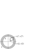
Figure 9. Scale of a mixed oval of depht $j$

Now we describe the positions of the ovals in the quadrants of $\mathbf{R}^{2}$ of a multi-Harnack smoothing $C_{{\underline{t}}_{1}}$ of a real plane branch $(C,0)$.

Definition 8.22.

We say that the signed topological type of a multi-Harnack smoothing $C_{{\underline{t}}_{1}}$ of a real plane branch $(C,0)$ is normalized if the signed topological type of the chart of $P^{\hat{\Delta}_{g}}_{t_{g}=1}$ is normalized (see Definition 6.6).

Proposition 8.23.

Let $C_{{\underline{t}}_{1}}$ be a multi-Harnack smoothing of a real plane branch $(C,0)$. If the signed topological type of the chart of $P_{\Delta_{g}}$ is normalized, then the same happens for the signed topological type of the chart $P^{\hat{\Delta}_{j}}_{t_{j}=1}$, for $j=1,\dots,g-1$.

Proof. The proof is by induction on $g$, using Proposition 8.13 and that $\pi_{1}(\mathbf{R}^{2}_{0,0})\subset\mathbf{R}^{2}_{0,0}$. $\Box$

We assume that the signed type of the smoothing is normalized. By the proof of Theorem 8.4 and the definition an oval of depth $j$ of $C_{{\underline{t}}_{1}}$ arises as a connected component $\Omega_{r,s}^{(j)}$ of the chart $\mbox{Ch}_{\Delta_{j}}(P^{\hat{\Delta}_{j}}_{t_{j}=1})$, for $(r,s)\in\mbox{\rm int}(\Delta_{j})\cap\mathbf{Z}^{2}$ (see Remark 4.6). An arc of a mixed oval of depth $j$ corresponds to a connected component $\Omega_{r,s}^{(j)}$ of the chart $\mbox{Ch}_{\Delta_{j}}(P^{\hat{\Delta}_{j}}_{t_{j}=1})$, for $(r,s)\in\Gamma_{j}\cap\mathbf{Z}^{2}$. Since at each stage the smoothing $C^{(j)}_{{\underline{t}}_{j}}$ of $C^{(j)}$ is multi-Harnack only the non compact component of the smoothing $C^{(j)}_{{\underline{t}}_{j}}$ meets the coordinate axis. Then we have the following:

Proposition 8.24.

If $C_{{\underline{t}}_{1}}$ is a normalized multi-Harnack smoothing of a real plane branch $(C,0)$ then we can label the ovals of depth $j$ (resp. the mixed ovals of depth $j$) by $O_{r,s}^{(j)}$ for $(r,s)\in\mbox{\rm int}(\Delta_{j})\cap\mathbf{Z}^{2}$ (resp. for $(r,s)\in\Gamma_{j}\cap\mathbf{Z}^{2}$). Then we have that $O_{r,s}^{(j)}\subset\mathbf{R}^{2}_{k,l}$ where

$$(k,l)=\left\{\begin{array}[]{ccc}(e_{0}+s,r)&\mbox{ if }&j=1\\ (e_{j-1}+s)n_{1}n_{2}\cdots n_{j-1},(e_{j-1}+s)m_{1}n_{2}\cdots n_{j-1})&if&1<j\leq g.\end{array}\right.$$

Proof. By hypothesis and Proposition 8.23 we have that the signed topological type of the chart of $P^{\hat{\Delta}_{j}}_{t_{j}=1}$ is normalized, for $j=1,\dots,g$. By Remark 6.5 we have that the component $\Omega_{r,s}^{(j)}$ of the chart $\mbox{\rm Ch}^{*}_{\Delta_{j}}(P^{\hat{\Delta}_{j}}_{t_{j}=1})$ is contained in the quadrant $\mathbf{R}^{2}_{e_{j-1}+s,r}$ with respect to the coordinates $(x_{j},y_{j})$. We abuse of notation and denote in the same way the component $\Omega_{r,s}^{(j)}$ of the chart $\mbox{\rm Ch}^{*}_{\Delta_{j}}(P^{\hat{\Delta}_{j}}_{t_{j}=1})$ and the corresponding connected component of the smoothing $C_{{\underline{t}}_{j}}^{(j)}\cap(\mathbf{R}^{*})^{2}$. By construction the oval $O_{r,s}^{(j)}$, which appears as a slight deformation of $\pi_{1}\circ\cdots\circ\pi_{j-1}(O_{r,s}^{(j)})$ of $\Omega_{r,s}^{(j)}$, is contained in the same quadrant $\mathbf{R}^{2}_{k,l}$ as $\pi_{1}\circ\cdots\circ\pi_{j-1}(\Omega_{r,s}^{(j)})$. Notice that on the oval $\pi_{i}\circ\cdots\circ\pi_{j-1}(\Omega_{r,s}^{(j)})$ the function $u_{i}\sim 1$, for $0<t_{i}\ll\cdots\ll t_{g}\ll 1$ by (18), for $1\leq i\leq j$. Then the assertion follows by the definition of the toric maps $\pi_{i}$ in (16). $\Box$

8.6. Examples

Example 8.25.

We consider first the constructions of a multi-Harnack smoothing of the real plane branch $(C,0)$ defined by the polynomial $F=(y^{2}-x^{3})^{3}-x^{10}$ studied in the Example 7.1 and 7.6. The Milnor number is equal to $44$.

The strict transform $C^{(2)}$ of $(C,0)$ is a simple cusp. Then a smoothing $C^{(2)}_{{\underline{t}}_{2}}$ of normalized type is of the form indicated in Figure 1. We indicate the form of the deformation $C_{{\underline{t}}_{2}}$ inside a Milnor ball $B$ for $(C,0)$ in Figure 10; the small circle denotes a Milnor ball $B^{\prime}$ for the singularity obtained. The smoothing $C_{{\underline{t}}_{1}}$ is the result of perturbing this singularity inside its Milnor ball and appears in Figure 11. Notice that the ovals which appear in the smaller ball are infinitesimally smaller than the others. In this example there is only one oval of depth $2$ and two mixed ovals of depth $1$.

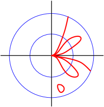
Figure 10. The deformation $C_{{\underline{t}}_{2}}$ inside the Milnor ball

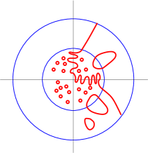
Figure 11. A multi-Harnack smoothing

Example 8.26.

We consider first the constructions of multi-Harnack smoothings of the real plane branch $(C,0)$ defined by the polynomial $F=(y^{2}-x^{3})^{4}-x^{12}y$. The Milnor number is equal to $86$.

By computing as in Section 2 we find that $g=2$, $(n_{1},m_{1})=(2,3)$ and $(n_{2},m_{2})=(4,3)$. It follows that the strict transform $C^{(2)}$ of $(C,0)$ has local Newton polygon with vertices $(0,4)$ and $(3,0)$. Figure 3 shows the signed topological types of a Harnack smoothing $C^{(2)}_{{\underline{t}}_{2}}$ of $(C^{(2)},o_{2})$. Then, the deformation $C_{{\underline{t}}_{2}}$, obtained by Proposition 8.13 is shown in Figure 12 (A) and (B) (notice that all the branches of the singularity at the origin have the same tangent line, the horizontal axis, though this is not represented in the Figure).

Then, if $C_{{\underline{t}}_{2}}$ defines a multi-Harnack smoothing of $(C,0)$ we have that $P^{\hat{\Delta}_{1}}_{t_{1}=1}(x,y)$ has the chart represented in Figure 13. The topology of the multi-Harnack smoothing is shown in Figure 14. Notice that, as stated in Theorem 8.4, the topological type of the resulting msqh-smoothing $C_{{\underline{t}}_{2}}$ is the same in cases (A) and (B) (meanwhile the signed topological types are different). The ovals inside the fist ball are of depth $1$, those intersecting the boundary are mixed ovals of depth $1$ and the ovals in between both balls are of depth $2$.

Example 8.27.

We show a Harnack smoothing of the real plane branch $(C,0)$ defined by the polynomial $F=(y^{2}-x^{3})^{7}-x^{24}$ which is not multi-Harnack.

By computing as in Section 2 we find that $g=2$, $(n_{1},m_{1})=(2,3)$ and $(n_{2},m_{2})=(7,6)$ and $\mu(C)_{0}=296$. It follows that the strict transform $C^{(2)}$ of $(C,0)$ has local Newton polygon with vertices $(0,7)$ and $(6,0)$.

We exhibit first a smoothing $C^{(2)}_{{\underline{t}}_{2}}$, defined by a degree seven curve with Newton polygon equal to $\Delta_{2}$. The construction begins by perturbing a degree four curve, composed of a smooth conic $C_{2}$ and two lines $L$ and $L^{\prime}$ in Figure 15 (a), with four lines, shown in grey, intersecting the conic in two real points (see [V3] for a summary of construction of real curves by small perturbations). The result is a smooth quartic $C_{4}$, as in Figure 15 (b), where we have indicated in gray the reference lines $L$ and $L^{\prime}$ with the conic $C_{2}$. Then we perturb the union of $C_{2}$ and $C_{4}$, by taking six lines, as in Figure 15 (c). The result is a $M$-sextic in maximal position with respect to the line $L$. The union of both curves is a degree seven curve $C_{7}$, as shown in Figure 15(d), where we indicate also the reference lines $L^{\prime}$ and $L^{\prime\prime}$. Notice that in Figures 15 (c) and (d). the line at infinity changes. See also the construction of curves corresponding to Figure 13 and 14 of [V3]. The result of a suitable perturbation of the singularities of $C_{7}$ is the $M$-degree seven curve shown in Figure 16 (e). Notice that this curve, which we call also $C_{7}$, is in maximal position with respect to the line $L^{\prime}$ and has maximal intersection multiplicity with the line $L$ at the point $L\cap L^{\prime\prime}$. It follows that a polynomial defining $C_{7}$, with respect to affine coordinates $(x,y)$ such that $x=0$ defines the line $L$, $y=0$ defines $L^{\prime}$ and $L^{\prime\prime}$ is the line at infinity, has generically Newton polygon with vertices $(0,0)$, $(7,0)$ and $(0,6)$, since $C_{7}$ passes by the point $L\cap L^{\prime\prime}$. The chart of $C_{7}$, with respect to its Newton polygon, is shown in Figure 16 (f).

We construct from the curve $C_{7}$ a sqh-smoothing $C^{(2)}_{{\underline{t}}_{2}}$ of $(C^{(2)},o_{2})$. By Proposition 8.13 the topology of the deformation $C_{{\underline{t}}_{2}}$ can be seen from the chart associated to $C_{{\underline{t}}_{2}}$ (compare Figures 16 (f) and 17 (g), where we have indicated by the same number the corresponding peripheral roots) We define then a msqh-Harnack smoothing $C_{{\underline{t}}_{1}}$ of $C_{{\underline{t}}_{2}}$ by gluing together the chart of $C_{{\underline{t}}_{2}}$ with the chart of a suitable Harnack smoothing of $(C_{{\underline{t}}_{2}},0)$ (see Theorem 6.1) . The topology of the msqh-Harnack smoothing $C_{{\underline{t}}_{1}}$ is shown in Figure 17 (h).

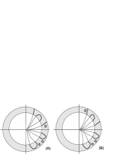
Figure 12. Figure (A) corresponds to the normalized case

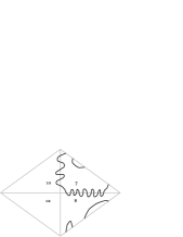
Figure 13. The numbers indicate the ovals to be added in the corresponding region

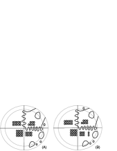
Figure 14.

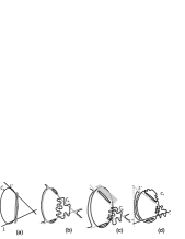
Figure 15.

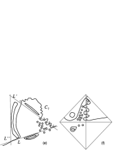
Figure 16.

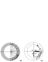
Figure 17.

Acknowledgement. The authors are grateful to Erwan Brugallé for suggesting example 8.27.

References

- [A’C-Ok] A’Campo, N., Oka, M.: Geometry of plane curves via Tschirnhausen resolution tower, Osaka J. Math., 33, (1996), 1003-1033.
- [A-M] Abhyankar, S.S., Moh, T.: Newton-Puiseux Expansion and Generalized Tschirnhausen Transformation I-II, J.Reine Angew. Math., 260. (1973), 47-83; 261. (1973), 29-54.
- [Ar] Arnold, V.I.: Some open problems in theory of singularities, Proc. Sobolev Seminar Novosibirsk; English transl., Singularities, Proc. Symp. Pure Math. (P.Orlik, ed.) vol 40, Part 1, Amer. Math. Soc. , Providence, RI, 1983, 57-69.
- [B] Bihan, F.: Viro method for the construction of real complete intersections, Adv. Math. 169 (2002), no. 2, 177-186.
- [Br] Brusotti, L.: Curve generatrici e curve aggregate nella costruzione di curve piane d’ordine assegnato dotate del massimo numero di circuiti, Rend. Circ. Mat. Palermo 42 (1917), 138-144.
- [Fu] Fulton, W.: Introduction to toric varieties, Annals of Mathematics Studies, 131. Princeton University Press, Princeton, NJ, 1993.
- [F-P-T] Forsberg, M., Passare, M., Tsikh, A.: Laurent determinants and arrangements of hyperplane amoebas, Adv. Math. 151 (2000), no. 1, 45–70.
- [GB-T] García Barroso, E., Teissier, B.: Concentration multi-échelles de courbure dans des fibres de Milnor Comment. Math. Helv. 74 (1999), 398-418.
- [GP1] González Pérez P.D.: Singularités quasi-ordinaires toriques et polyèdre de Newton du discriminant, Canadian J. Math. 52 (2), 2000, 348-368.
- [GP2] González Pérez, P.D.: Approximate roots, toric resolutions and deformations of a plane branch, Manuscript 2008.
- [GP] González Pérez, P.D.: Toric embedded resolutions of quasi-ordinary hypersurface singularities. Ann. Inst. Fourier (Grenoble) 53, 6, (2003), 1819–1881.
- [G-T] Goldin, R., Teissier, B.: Resolving singularities of plane analytic branches with one toric morphism, Resolution of Singularities, A research textbook in tribute to Oscar Zariski. Edited by H. Hauser, J. Lipman, F.Oort and A. Quiros. Progress in Mathematics No. 181, Birkhäuser-Verlag, 2000, 315-340.
- [G-K-Z] Gel’fand, I.M., Kapranov, M.M. Zelevinsky, A.V.: Discriminants, Resultants and Multi-Dimensional Determinants, Birkhäuser, Boston, 1994.
- [I-V] Itenberg, I., Viro, O.Ya.: Patchworking algebraic curves disproves the Ragsdale conjecture, Math. Intelligencer 18 (1996), no. 4, 19–28.
- [I1] Itenberg, I.: Amibes de variétés algébriques et dénombrement de courbes (d’après G. Mikhalkin), Asterisque 921, (2003), 335–361.
- [I2] Itenberg, I.: Viro’s method and T-curves, Algorithms in Algebraic Geometry and its applications (Santander 1994), 177-192, Prog. Math. 143, Birkhäuser Basel 1996.
- [K-O-S] Kharlamov, V. M., Orevkov, S. Yu., Shustin, E. I.: Singularity which has no -smoothing, The Arnoldfest (Toronto, ON, 1997), 273-309, Fields Inst. Commun., 24, Amer. Math. Soc., Providence, RI, 1999.
- [K-R] Kharlamov, V. M., Risler, J-J.: Blowing-up construction of maximal smoothings of real plane curve singularities, Real analytic and algebraic geometry (Trento, 1992), 169–188, de Gruyter, Berlin, 1995.
- [K-R-S] Kharlamov, V., Risler, J-J., Shustin, E.: Maximal smoothings of real plane curve singular points, Topology, ergodic theory, real algebraic geometry, 167–195, Amer. Math. Soc. Transl. Ser. 2, 202, Amer. Math. Soc., Providence, RI, 2001.
- [Kou] Kouchnirenko, A.G.: Polyèdres de Newton et nombres de Milnor, Invent. Math., 32, (1976), 1-31.
- [Kh] Khovanskii, A.C.: Newton polyhedra and the genus of complete intersections, Funktsional Anal. i Prilozhen 12 (1978), no.1, 51-61; English transl. Functional Anal. Appl. 12 (1978), no. 1, 38-46.
- [L-Ok] Lê D.T., Oka, M.: On resolution complexity of plane curves, Kodai Math. J. 18 (1995), no. 1, 1–36.
- [Mil] Milnor, J.: Singular points of complex hypersurfaces, Annals of Mathematics Studies, No. 61 Princeton University Press, Princeton, N.J. 1968
- [M] Mikhalkin, G.: Real algebraic curves, the moment map and amoebas, Ann. of Math. (2) 151 (2000), no. 1, 309-326.
- [M-R] Mikhalkin, G., Rullgard, H.: Amoebas of maximal area, Internat. Math. Res. Notices, 2001, no. 9, 441-451.
- [Od] Oda, T.: Convex Bodies and Algebraic Geometry, Annals of Math. Studies (131), Springer-Verlag, 1988.
- [Ok1] Oka, M.: Geometry of plane curves via toroidal resolution, Algebraic Geometry and Singularities, Progress in Mathematics No. 139, Birkhäuser, Basel, 1996.
- [Ok2] Oka, M.: Non-degenerate complete intersection singularity, Actualités Mathematiques, Hermann, Paris, 1997.
- [P-R] Passare, M., Rullgard, H.: Amoebas, Monge-Ampère measures, and triangulations of the Newton polytope, Duke Math. J., 121 (2004), no. 3, 481-507.
- [PP] Popescu-Pampu, P.: Approximate roots, Valuation theory and its applications, Vol. II (Saskatoon, SK, 1999), Fields Inst. Commun., 33, Amer. Math. Soc., Providence, RI, 2003, 285-321.
- [R1] Risler, J-J.: Construction d’hypersurfaces réelles (d’après Viro), Séminaire Bourbaki, Vol. 1992/93. Astérisque No. 216 (1993), Exp. No. 763, 3, 69-86.
- [R2] Risler, J-J.: Un analogue local du théorème de Harnack, Invent. Math., 89 (1987), no. 1, 119-137.
- [St] Sturmfels, B.: Viro’s theorem for complete intersections, Ann. Scuola Norm. Sup. Pisa Cl. Sci. (4) 21 (1994), no. 3, 377-386.
- [V1] Viro, O.Ya.: Gluing of algebraic hypersurfaces, smoothing of singularities and construction of curves (in Russian), Proceedings of the Leningrad Internacional Topological Conference (Leningrad 1982) , Nauka, Leningrad, 1983, 149-197.
- [V2] Viro, O.Ya.: Gluing of plane real algebraic curves and constructions of curves of degrees and , Topology (Leningrad, 1982), Lecture Notes in Math., 1060, Springer, 1984, 187-200.
- [V3] Viro, O.Ya.: Real plane algebraic curves: constructions with controlled topology, Leningrad Math. J. 1 (1990), no. 5, 1059-1134.
- [V4] Viro, O.Ya.: Patchworking real algebraic varieties, U.U.D.M. Report 1994, 42, Uppsala University, 1994.
- [Z2] Zariski, O.: Le problème des modules pour les branches planes, Hermann, Paris, 1986.