Optical realization of a quantum beam splitter

R. Mar-Sarao and H. Moya-Cessa INAOE, Apdo. Postal 51 y 216, 72000, Puebla, Pue., Mexico
Abstract

We show how the quantum process of splitting light may be modelled in classical optics. A second result is the possibility to engineer specific forms of a classical field.

.1 Introduction

The modelling of quantum mechanical systems with classical optics is a topic that has attracted interest recently. Along these lines Man’ko et al. have proposed to realize quantum computation by quantum like systems Mank and Crasser et al. Sch have pointed out the similarities between quantum mechanics and Fresnel optics in phase space. Following these cross-applications, here we would like to show how a quantum beam splitter may be modelled in classical optics. The possibility of generating specific forms (engineering) of the propagated field is also studied.

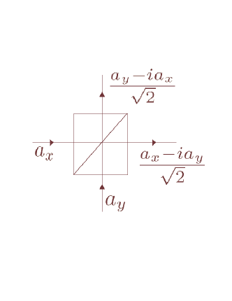
A beam splitter is an optical component that combines two propagating modes into two other propagating modes. Fig. 1 shows the setup that produces this effect for a 50:50 beam splitter. Two fields $a_{x}$ and $a_{y}$ enter the beam splitter and two fields exit it, that correspond to a combination of the entering ones. In quantum optics the beam splitter is modelled by the interaction of two fields Villas with the Hamiltonian given by

H=Ο‰x​ax†​ax+Ο‰y​ay†​ay+χ​(ay†​ax+ax†​ay)𝐻subscriptπœ”π‘₯superscriptsubscriptπ‘Žπ‘₯†subscriptπ‘Žπ‘₯subscriptπœ”π‘¦superscriptsubscriptπ‘Žπ‘¦β€ subscriptπ‘Žπ‘¦πœ’superscriptsubscriptπ‘Žπ‘¦β€ subscriptπ‘Žπ‘₯superscriptsubscriptπ‘Žπ‘₯†subscriptπ‘Žπ‘¦H=\omega_{x}a_{x}^{\dagger}a_{x}+\omega_{y}a_{y}^{\dagger}a_{y}+\chi(a_{y}^{\dagger}a_{x}+a_{x}^{\dagger}a_{y}) (1)

where the $\omega$’s are the field frequencies, $\chi$ is the interaction constant and $a_{j}$ and aj†superscriptsubscriptπ‘Žπ‘—β€ a_{j}^{\dagger} ($j=x,y$) are the annihilation and creation operators of the field modes.

If we consider equal field frequencies, we can obtain the beam splitter operator Campos

B=eβˆ’i​θ​(ay†​ax+ax†​ay)𝐡superscriptπ‘’π‘–πœƒsuperscriptsubscriptπ‘Žπ‘¦β€ subscriptπ‘Žπ‘₯superscriptsubscriptπ‘Žπ‘₯†subscriptπ‘Žπ‘¦B=e^{-i\theta(a_{y}^{\dagger}a_{x}+a_{x}^{\dagger}a_{y})} (2)

with $\theta=\chi t$. Note that

B​ax​B†=cos⁑(ΞΈ)​ax+i​sin⁑(ΞΈ)​ay,𝐡subscriptπ‘Žπ‘₯superscriptπ΅β€ πœƒsubscriptπ‘Žπ‘₯π‘–πœƒsubscriptπ‘Žπ‘¦\displaystyle Ba_{x}B^{\dagger}=\cos(\theta)a_{x}+i\sin(\theta)a_{y},
B​ay​B†=cos⁑(ΞΈ)​ay+i​sin⁑(ΞΈ)​ax𝐡subscriptπ‘Žπ‘¦superscriptπ΅β€ πœƒsubscriptπ‘Žπ‘¦π‘–πœƒsubscriptπ‘Žπ‘₯\displaystyle Ba_{y}B^{\dagger}=\cos(\theta)a_{y}+i\sin(\theta)a_{x} (3)

such that $\cos(\theta)$ and $\sin(\theta)$ may be related directly with the transmission and reflection coefficients. One feature present in the quantum beam splitter is that, if there is only one field entering by one of the arms of the beam splitter, one has to consider always a vacuum field entering by the other arm. It is well known that this system produces entanglement Kim ; Scheel , for instance, if we consider the 50:50 beam splitter, i.e. we set $\theta=\pi/4$, (see Fig. 1) and in each of the arms the first excited number state, namely the state $|\psi_{I}\rangle=|1\rangle_{x}|1\rangle_{y}$ as initial state, we have as final state

$$|\psi_{F}\rangle=\frac{i}{\sqrt{2}}(|2\rangle_{x}|0\rangle_{y}+|0\rangle_{x}|2\rangle_{y}),$$ (4)

this is an entangled state that tells that both photons travel together.

.2 Modelling field-field interaction

We consider the paraxial propagation of a field, that has the equation form (see for instance Chavez

$$2ik_{0}\frac{\partial E}{\partial z}=\nabla_{\perp}^{2}E+k^{2}(x,y)E$$ (5)

where $k_{0}=2\pi n_{0}/\lambda$ is the wavenumber with $\lambda$ the wavelength of the propagating lightbeam, $n_{0}$ is the homogeneous refractive index. The function $k^{2}(x,y)$ describes the inhomogeneity of a medium responsible for the waveguiding of an optical field $E$. It has been recently shown that by using an astigmatic and slightly tilted probe beam, it produces a GRIN like medium, with an extra cross term $\chi xy$ Chavez . Taking into account such inhomogeneity the paraxial wave equation is written as

$\displaystyle i\frac{\partial E}{\partial z}=\frac{\nabla_{\perp}^{2}}{2k_{0}}E$ (6)
$\displaystyle+$ $\displaystyle\left(k_{0}/2-\frac{1}{2}(k_{0}\tilde{\alpha}_{x}^{2}x^{2}+k_{0}\tilde{\alpha}_{y}^{2}y^{2})+\chi xy\right)E,$

with $k_{0}\tilde{\alpha}_{q}^{2},\qquad q=x,y$ inhomogeneity parameters related to the generated GRIN medium Chavez .

.3 Optical realization of the quantum beam splitter

Let us define the ladder operators Arfken

$\displaystyle a_{q}=\sqrt{\frac{k_{0}\tilde{\alpha}_{q}}{2}}q+\frac{1}{\sqrt{2k_{0}\tilde{\alpha}_{q}}}\frac{d}{dq},$
aq†=k0​α~q2​qβˆ’12​k0​α~q​dd​q,superscriptsubscriptπ‘Žπ‘žβ€ subscriptπ‘˜0subscript~π›Όπ‘ž2π‘ž12subscriptπ‘˜0subscript~π›Όπ‘žπ‘‘π‘‘π‘ž\displaystyle a_{q}^{\dagger}=\sqrt{\frac{k_{0}\tilde{\alpha}_{q}}{2}}q-\frac{1}{\sqrt{2k_{0}\tilde{\alpha}_{q}}}\frac{d}{dq}, (7)

with $q=x,y$. These operators are also called creation and annihilation operators in quantum optics because the action of $a_{x}$ on a function

$$u_{m}(x)=\left(\frac{k_{0}\tilde{\alpha}_{x}}{\pi}\right)^{1/4}\frac{1}{\sqrt{2^{m}m!}}H_{m}(\sqrt{k_{0}\tilde{\alpha}_{x}}x)e^{-k_{0}\tilde{\alpha}_{x}x^{2}/2}$$ (8)

where $H_{m}(x)$ are Hermite polynomials, gives

$$a_{x}u_{m}(x)=\sqrt{m}u_{m-1}(x)$$ (9)

and

$$a_{x}^{\dagger}u_{m}(x)=\sqrt{m+1}u_{m+1}(x).$$ (10)

The above equations are also valid for the $y$ coordinate simply making the change $y\rightarrow x$. Furthermore, note that $[a_{x},a_{x}^{\dagger}]=1$. We can rewrite (6) using (7) as

$\displaystyle i\frac{\partial E}{\partial z}=\left(\tilde{\alpha}_{x}(n_{x}+\frac{1}{2})+\tilde{\alpha}_{y}(n_{y}+\frac{1}{2})+\chi xy+\frac{k_{0}}{2}\right)E,$ (11)

with nj=aj†​ajsubscript𝑛𝑗superscriptsubscriptπ‘Žπ‘—β€ subscriptπ‘Žπ‘—n_{j}=a_{j}^{\dagger}a_{j} for $j=x,y$ the so-called number operator. We transform (11) to get rid of the constant terms, via $\psi=\exp[-iz(\tilde{\alpha}_{x}+\tilde{\alpha}_{y}+k_{0})/2]E$, and we assume $\chi\ll\tilde{\alpha}_{x},\tilde{\alpha}_{y}$ so we can perform the so-called rotating wave approximation (see for instance Moya ) to finally obtain

iβ€‹βˆ‚Οˆβˆ‚z=(Ξ±~x​nx+Ξ±~y​ny+Ο‡~​(ax​ay†+ax†​ay))β€‹Οˆ,π‘–πœ“π‘§subscript~𝛼π‘₯subscript𝑛π‘₯subscript~𝛼𝑦subscript𝑛𝑦~πœ’subscriptπ‘Žπ‘₯superscriptsubscriptπ‘Žπ‘¦β€ superscriptsubscriptπ‘Žπ‘₯†subscriptπ‘Žπ‘¦πœ“i\frac{\partial\psi}{\partial z}=\left(\tilde{\alpha}_{x}n_{x}+\tilde{\alpha}_{y}n_{y}+\tilde{\chi}(a_{x}a_{y}^{\dagger}+a_{x}^{\dagger}a_{y})\right)\psi, (12)

with $\tilde{\chi}=\frac{\chi}{2k_{0}\sqrt{\tilde{\alpha_{x}}\tilde{\alpha_{y}}}}$. This equation is equivalent to the field-field interaction in quantum optics Dutra .

Refer to caption
Figure 1: Configuration of the beam splitter (50:50) operation.

We do a last transformation $\phi=\exp[-iz\tilde{\alpha}_{x}(n_{x}+n_{y})]\psi$ and obtain

iβ€‹βˆ‚Ο•βˆ‚z=[Δ​ny+Ο‡~​(ax​ay†+ax†​ay)]​ϕ≑H​ϕ,𝑖italic-ϕ𝑧delimited-[]Ξ”subscript𝑛𝑦~πœ’subscriptπ‘Žπ‘₯superscriptsubscriptπ‘Žπ‘¦β€ superscriptsubscriptπ‘Žπ‘₯†subscriptπ‘Žπ‘¦italic-ϕ𝐻italic-Ο•i\frac{\partial\phi}{\partial z}=[\Delta n_{y}+\tilde{\chi}(a_{x}a_{y}^{\dagger}+a_{x}^{\dagger}a_{y})]\phi\equiv H\phi, (13)

with $\Delta=\tilde{\alpha}_{y}-\tilde{\alpha}_{x}$. It is useful to define ”normal-mode” operators by Dutra

$${A_{1}}=\delta a_{x}+\gamma a_{y},\qquad A_{2}=\gamma a_{x}-\delta a_{y},$$ (14)

with

$$\delta=\frac{2\tilde{\chi}}{\sqrt{2\Omega(\Omega-\Delta)}},\qquad\gamma=\sqrt{\frac{\Omega-\Delta}{2\Omega}},\qquad\delta^{2}+\gamma^{2}=1$$ (15)

with $\Omega=\sqrt{\Delta^{2}+4\tilde{\chi}^{2}}$ the Rabi frequency. ${A_{1}}$ and $A_{2}$ are annihilation operators just like $a$ and $b$ and obey the commutation relations

$$[{A_{1}},{A_{1}}^{\dagger}]=[A_{2},A_{2}^{\dagger}]=1,$$ (16)

moreover, the normal-mode operators commute with each other

$$[{A_{1}},A_{2}]=[{A_{1}},A_{2}^{\dagger}]=0.$$ (17)

In terms of these operator $H$ in (13) becomes

$$H=\mu_{1}A_{1}^{\dagger}{A_{1}}+\mu_{2}{A}_{2}^{\dagger}{A}_{2},$$ (18)

with $\mu_{1,2}=(\Delta\pm\Omega)/2$. In order to have a way of transforming functions from one basis to the other, we note that the lowest functions $u_{0}(x)u_{0}(y)$ are also eigenfunctions of the normal-mode operators

$$A_{m}u_{0}(x)u_{0}(y)=0,\qquad m=1,2,$$ (19)

i.e. they are the lowest states, up to a phase, in the new basis Dutra

$$u_{0}(x)u_{0}(y)=U_{0}^{1}(x,y)U_{0}^{2}(x,y).$$ (20)

.3.1 Initial function $u_{1}(x)u_{1}(y)$

If we consider

$$\phi(z=0;x,y)=u_{1}(x)u_{1}(y)$$ (21)

the propagated function reads

ϕ​(z;x,y)=eβˆ’i​z​(ΞΌ1​A1†​A1+ΞΌ2​A2†​A2)​ax†​ay†​u0​(x)​u0​(y),italic-ϕ𝑧π‘₯𝑦superscript𝑒𝑖𝑧subscriptπœ‡1superscriptsubscript𝐴1†subscript𝐴1subscriptπœ‡2superscriptsubscript𝐴2†subscript𝐴2subscriptsuperscriptπ‘Žβ€ π‘₯subscriptsuperscriptπ‘Žβ€ π‘¦subscript𝑒0π‘₯subscript𝑒0𝑦\phi(z;x,y)=e^{-iz(\mu_{1}A_{1}^{\dagger}{A_{1}}+\mu_{2}{A}_{2}^{\dagger}{A}_{2})}a^{\dagger}_{x}a^{\dagger}_{y}u_{0}(x)u_{0}(y), (22)

by writing the creation operators in terms of creation operators for the normal-modes, (14), we obtain

ϕ​(z;x,y)=eβˆ’i​z​μ1​A1†​A1​eβˆ’i​z​μ2​A2†​A2​(δ​A1†+γ​A2†)​(γ​A1β€ βˆ’Ξ΄β€‹A2†)​U01​(x,y)​U02​(x,y).italic-ϕ𝑧π‘₯𝑦superscript𝑒𝑖𝑧subscriptπœ‡1superscriptsubscript𝐴1†subscript𝐴1superscript𝑒𝑖𝑧subscriptπœ‡2superscriptsubscript𝐴2†subscript𝐴2𝛿subscriptsuperscript𝐴†1𝛾subscriptsuperscript𝐴†2𝛾subscriptsuperscript𝐴†1𝛿subscriptsuperscript𝐴†2superscriptsubscriptπ‘ˆ01π‘₯𝑦superscriptsubscriptπ‘ˆ02π‘₯𝑦\phi(z;x,y)=e^{-iz\mu_{1}A_{1}^{\dagger}{A_{1}}}e^{-iz\mu_{2}{A}_{2}^{\dagger}{A}_{2}}(\delta A^{\dagger}_{1}+\gamma A^{\dagger}_{2})(\gamma A^{\dagger}_{1}-\delta A^{\dagger}_{2})U_{0}^{1}(x,y)U_{0}^{2}(x,y). (23)

Now we use the properties $e^{-iz\mu_{j}A_{j}^{\dagger}{A_{j}}}A^{\dagger}_{j}e^{iz\mu_{j}A_{j}^{\dagger}{A_{j}}}=A^{\dagger}_{j}e^{-iz\mu_{j}}$ and $e^{-iz\mu_{j}A_{j}^{\dagger}{A_{j}}}U^{j}_{0}(x,y)=U^{j}_{0}(x,y)$ to obtain

$$\phi(z;x,y)=(\delta A^{\dagger}_{1}e^{-iz\mu_{1}}+\gamma A^{\dagger}_{2}e^{-iz\mu_{2}})(\gamma A^{\dagger}_{1}e^{-iz\mu_{1}}-\delta A^{\dagger}_{2}e^{-iz\mu_{2}})U_{0}^{1}(x,y)U_{0}^{2}(x,y),$$ (24)

that in the old basis reads

ϕ​(z;x,y)=[η​(z)​β​(z)​ax†2+ϡ​(z)​β​(z)​ay†2+(Ξ²2​(z)+ϡ​(z)​η​(z))​ax†​ay†]​u0​(x)​u0​(y),italic-ϕ𝑧π‘₯𝑦delimited-[]πœ‚π‘§π›½π‘§subscriptsuperscriptπ‘Žβ€ absent2π‘₯italic-ϡ𝑧𝛽𝑧subscriptsuperscriptπ‘Žβ€ absent2𝑦superscript𝛽2𝑧italic-Ο΅π‘§πœ‚π‘§subscriptsuperscriptπ‘Žβ€ π‘₯subscriptsuperscriptπ‘Žβ€ π‘¦subscript𝑒0π‘₯subscript𝑒0𝑦\phi(z;x,y)=[\eta(z)\beta(z)a^{\dagger 2}_{x}+\epsilon(z)\beta(z)a^{\dagger 2}_{y}+(\beta^{2}(z)+\epsilon(z)\eta(z))a^{\dagger}_{x}a^{\dagger}_{y}]u_{0}(x)u_{0}(y), (25)

with $\eta(z)=\delta^{2}e^{-iz\mu_{1}}+\gamma^{2}e^{-iz\mu_{2}}$, $\beta(z)=\gamma\delta(e^{-iz\mu_{1}}-e^{-iz\mu_{2}})$ and $\epsilon(z)=\delta^{2}e^{-iz\mu_{2}}+\gamma^{2}e^{-iz\mu_{1}}$. The term that multiplies ax†​ay†subscriptsuperscriptπ‘Žβ€ π‘₯subscriptsuperscriptπ‘Žβ€ π‘¦a^{\dagger}_{x}a^{\dagger}_{y} may be written as

$$e^{-i\Delta z}[(\gamma^{2}-\delta^{2})^{2}+4\gamma^{2}\delta^{2}\cos(\Omega z)],$$

oscillates crossing zero periodically. By looking at the propagated field at one of these zeros (at $z_{0}$), a state of the form (4) is obtained, i.e.

$$\phi(z_{0};x,y)=\eta(z_{0})\beta(z_{0})u_{2}(x)u_{0}(y)+\epsilon(z_{0})\beta(z_{0})u_{0}(x)u_{2}(y).$$ (26)

.3.2 SU(2) coherent state

One can engineer functions in the form of determined superpositions of the functions (8). For instance, one can engineer the so-called SU(2) coherent state by setting the functions $u_{m}(x)$ and $u_{0}(y)$ at the plane $z=0$

$$\phi(z=0;x,y)=u_{m}(x)u_{0}(y)=\frac{a_{x}^{\dagger m}}{\sqrt{m!}}u_{0}(x)u_{0}(y),$$ (27)

that after application of the propagator $e^{-iz(\mu_{1}A_{1}^{\dagger}{A_{1}}+\mu_{2}{A}_{2}^{\dagger}{A}_{2})}$ gives

ϕ​(z;x,y)=(η​(z)​ax†+β​(z)​ay†)mm!​u0​(x)​u0​(y),italic-ϕ𝑧π‘₯𝑦superscriptπœ‚π‘§superscriptsubscriptπ‘Žπ‘₯†𝛽𝑧superscriptsubscriptπ‘Žπ‘¦β€ π‘šπ‘šsubscript𝑒0π‘₯subscript𝑒0𝑦\phi(z;x,y)=\frac{(\eta(z)a_{x}^{\dagger}+\beta(z)a_{y}^{\dagger})^{m}}{\sqrt{m!}}u_{0}(x)u_{0}(y), (28)

that may be rewritten as the SU(2) coherent state Buzek ; Wod

$$\phi(z;x,y)=\sum_{n=0}^{m}\left(\begin{array}[]{l}m\\ n\end{array}\right)^{1/2}\eta^{m-n}(z)^{n}\beta(z)u_{m-n}(x)u_{n}(y).$$ (29)

.3.3 Gaussian function

Consider now that at $z=0$ we have a displaced Gaussian function as a function of $x$ and a function $u_{0}(y)$,

$$\phi(z=0;x,y)=\left(\frac{k_{0}\tilde{\alpha}_{x}}{{\pi}}\right)^{1/4}{e^{-{(\alpha-x\sqrt{\frac{k_{0}\tilde{\alpha}_{x}}{2}})^{2}}}}u_{0}(y)\equiv e^{-\frac{\alpha^{2}}{2}}\sum_{n}^{\infty}\frac{\alpha^{n}}{\sqrt{n!}}u_{n}(x)u_{0}(y),$$ (30)

by using the Glauber displacement operatorGlauber , this function may be rewritten as

$$\phi(z=0;x,y)=D_{a_{x}}(\alpha)u_{0}(x)u_{0}(y),$$ (31)

with Dax​(Ξ±)=exp⁑[α​(axβ€ βˆ’ax)]subscript𝐷subscriptπ‘Žπ‘₯𝛼𝛼superscriptsubscriptπ‘Žπ‘₯†subscriptπ‘Žπ‘₯D_{a_{x}}(\alpha)=\exp[\alpha(a_{x}^{\dagger}-a_{x})]. After application of the propagator operator, the propagated field reads

$$\phi(z;x,y)=D_{a_{x}}[\alpha\eta(z)]u_{0}(x)D_{a_{y}}[\alpha\beta(z)]u_{0}(y).$$ (32)

The electromagnetic field then will be displaced Gaussians in $x$ and $y$ dimensions, the initial Gaussians at $z=0$ will exchange displacement, i.e. the displaced Gaussian (that depends on $x$) will periodically diminish its displacement and back, while the one centered at $y=0$ will periodically be displaced and back to the origin.

.4 Conclusions

We have shown how to model a quantum beam splitter by propagating electromagnetic fields. Specific electromagnetic fields may be engineered by using this modelling, in particular we have shown how SU(2) coherent functions may be realized.

References

  • (1) M. A. Man’ko, V. I. Man’ko and R. Vilela Mendes, β€œQuantum computation by quantumlike systems,” Phys. Lett. A 288, 132-138 (2001).
  • (2) O. Crasser, H. Mack, and W. P. Schleich, β€œCould Fresnel optics be quantum mechanics in phase space?,” Fluctuation and Noise Letters 4, L43-L51 (2004).
  • (3) F. O. Prado, N. G. de Almeida, M. H. Y. Moussa, and C. J. Villas-BΓ΄as, ”Bilinear and quadratic Hamiltonians in two-mode cavity quantum electrodynamics,” Phys. Rev. A 73, 043803 (2008).
  • (4) R.A. Campos, B.E.A. Saleh, and M. C. Teich, ”Quantum-mechanical lossless beam splitter: SU(2) symmetry and photon statistics,” Phys. Rev. A 40, 1371-1384 (1989).
  • (5) M.S. Kim, W. Son, V. Buzek, and P.L. Knight, ”Entanglemenrt by a beam splitter: Nonclassicality as a prerequisite for entanglement” Phys. Rev. A 65, 032323 (2002).
  • (6) S. Scheel and D.-G- Welsch, ”Entanglement generation and degradation by passive optical devices,” Phys. Rev. A 64, 063811 (2001).
  • (7) S. Chavez-Cerda, J.R. Moya-Cessa, and H. Moya-Cessa, ”Quantumlike systems in classical optics: applications of quantum optical methods,” J. Opt. Soc. Am. B 24, 404-407 (2007).
  • (8) G. Arfken, Mathematical methods for physicists, (Academic Press, Inc. 1985), p. 720.
  • (9) H. Moya-Cessa, ”Decoherence in atom-field interactions: A treatment using superoperator techniques,” Phys. Rep. 432, 1-41 (2006).
  • (10) S.M. Dutra, P.L. Knight and H. Moya-Cessa, ”Discriminating Field Mixtures from Macroscopic Superpositions,” Phys. Rev. A 48, 3168-3173 (1993).
  • (11) V. Buzek and T. Quang, ”Generalized coherent state for bosonic realization of SU(2) Lie algebra,” J. Opt. Soc. Am. B 6, 2447 (1989).
  • (12) K. Wodkiewicz and J. H. Eberly, ”Coherent states, squeezed fluctuations, and the SU(2) and SU(1,1) groups in quantum-optics applications,” J. Opt. Soc. Am. B 3, 458 (1985).
  • (13) R.J. Glauber, ”Coherent and incoherent states of the radiation field,” Phys. Rev. 131, 2766-2788 (1963).