DMT of Multi-hop Cooperative Networks - Part I: Basic Results

Abstract

In this two-part paper, the DMT of cooperative multi-hop networks is examined. The focus is on single-source single-sink (ss-ss) multi-hop relay networks having slow-fading links and relays that potentially possess multiple antennas. In this first part, some basic results that help in determining the DMT of cooperative networks as well as in characterizing the two end-points of the DMT for arbitrary full-duplex networks is established. In the companion paper, two families of half-duplex networks are studied.

The present paper examines the two end-points of the DMT of ss-ss networks. In particular, the maximum achievable diversity of arbitrary multi-terminal wireless networks is shown to be equal to the min-cut between the corresponding source and the sink. The maximum multiplexing gain (MMG) of arbitrary full-duplex ss-ss networks is shown to be equal to the min-cut rank, using a new connection to a deterministic network for which the capacity was recently found. This connection is operational in the sense that a capacity-achieving scheme for the deterministic network can be converted into a MMG-achieving scheme for the original network.

We also prove some basic results including a proof that the colored noise encountered in AF protocols for cooperative networks can be treated as white noise for DMT computations. We derive lower bounds for the DMT of triangular channel matrices, which are subsequently utilized to derive alternative, and often simpler proofs of several existing results. The DMT of a parallel channel with independent MIMO links is also computed here. As an application of these basic results, we prove that a linear tradeoff between maximum diversity and maximum multiplexing gain is achievable for arbitrary, ss-ss single-antenna, directed-acyclic networks equipped with full-duplex relays.

All protocols in this paper are explicit and rely only upon amplify-and-forward (AF) relaying. Explicit codes for all protocols introduced here are included in the companion paper.

I Introduction

In fading relay networks, cooperative diversity provides a means of operating the network efficiently. While much of the work in the literature on cooperative diversity is based on two-hop networks, the attention here is on multi-hop networks.

I-A Prior Work

The concept of user cooperative diversity was introduced in [2]. Cooperative diversity protocols were first discussed in [3] for the two-hop, single-relay network (Fig.1(a)). Zheng and Tse [4] proposed the Diversity-Multiplexing gain Tradeoff (DMT) as a means of evaluating point-to-point, multiple-antenna schemes in the context of slow-fading channels.

I-A1 Two-hop Networks

The DMT was also used as a tool to compare various protocols for half-duplex two-hop cooperative networks in [5, 6]. As noted in [9], the DMT is simple enough to be analytically tractable and powerful enough to compare different cooperative-relay-network protocols. For any network, an upper bound on the achievable DMT is given by the cut-set bound [49, 9]. A fundamental question in this area is whether the cut-set bound on DMT can be achieved. While this question has been studied extensively for the two-hop cooperative wireless system in Fig.1(a), the question still remains open even for this class of network (see [10], [12] for a detailed comparison of existing achievable regions).

In [5], the selection-decode-and-forward protocol is analyzed for an arbitrary number of relays, where the authors give upper and lower bounds on the DMT of the protocol. In these protocols, the relays and the source node participate for equal time instants and the maximum multiplexing gain $r$ achieved is equal to $0.5$.

(a) General two-hop relay network

(b) Single relay network

Figure 1: Two-hop cooperative relay networks

In [6], Azarian et al. analyze the class of Non Orthogonal, Amplify-and-Forward (NAF) protocols, introduced earlier by Nabar et al. in [7] and establish the improved DMT of the NAF protocol in comparison to the class of Orthogonal-Amplify-and-Forward (OAF) protocols considered in [5]. It has been shown in [10], that the DMT of the NAF protocol can be obtained via the OAF protocol as well using appropriate unequal slot lengths for source and relay transmissions.

The authors of [6] also introduce the Dynamic Decode-and-Forward (DDF) protocol wherein the time duration for which the relays listen to the source depends on the source-relay channel gain. They show that for the single-relay case, the DMT of the DDF protocol achieves the cut-set bound (also known as the transmit-diversity bound) for $r\leq 0.5$, beyond which the DMT falls below the bound. An enhanced DDF protocol is proposed in [12] that improves upon DDF. However the DMT of this protocol also falls short of the transmit bound for $r\geq 0.5$.

Yang and Belfiore consider a class of protocols called Slotted-Amplify-And-Forward (SAF) protocols in [19] for the two-hop network with direct link, and show that these improve upon the performance of the NAF protocol [6] for the case of two relays. Under the assumption of relay isolation, the naive SAF scheme proposed in [19] is shown to achieve the cut-set bound. It is also conjectured in [19] that SAF protocol is optimal even when the relays are not isolated.

Yuksel and Erkip in [9] have considered the DMT of the DF and compress-and-forward (CF) protocols. They show that the CF protocol achieves the transmit-diversity bound for the case of a single relay. We note, however, that in the CF protocol, the relays are assumed to know all the fading coefficients in the system. The authors also translate cut-set upper bounds in [49] for mutual information into the DMT framework for a general multi-terminal network.

Jing and Hassibi [8] consider cooperative communication protocols for the two-hop network without a direct link between source and destination. They study protocols where the relay nodes apply a linear transformation to the received signal and analyze their BER performance. The authors consider the case when the source and the relays transmit for an equal number of channel uses and the relays perform a unitary transformation on the input symbols before transmitting it. Rao and Hassibi [28] consider two-hop half-duplex multi-antenna cooperative networks without direct link and provide an AF scheme and compute the DMT achieved by the scheme. Their scheme incurs a rate loss of a factor of two compared to the cut-set bound. In a parallel work [30], the DMT of the two-hop network without direct link is proved to be equal to the cut-set bound.

I-A2 Multi-hop Networks

Yang and Belfiore in [18] consider AF protocols for a family of MIMO multi-hop networks (which are termed as multi-antenna layered networks in the current paper). They derive the optimal DMT for the Rayleigh-product channel which they prove is equal to the DMT of the AF protocol applied to this channel. They also propose AF protocols to achieve the optimal diversity of these multi-antenna layered networks.

Oggier and Hassibi [40] have proposed distributed space time codes for multi-antenna layered networks that achieve diversity gain equal to the minimum number of relay nodes among the hops. Recently, Vaze and Heath [41] have constructed distributed space time codes based on orthogonal designs that achieve the optimal diversity of the multi-antenna layered network with low decoding complexity. In [42], the same authors study the circumstances under which full diversity can be achieved without coding in a layered network in the presence of partial CSIT.

Borade, Zheng and Gallager in [27] consider AF schemes on a class of multi-hop layered networks where each layer has the same number of relays (termed as regular networks in the current paper). They show that AF strategies are optimal in terms of multiplexing gain. They also compute lower bounds on the DMT of the product Rayleigh channel.

I-A3 Capacity

There has been a recent interest in determining approximations to the capacity of wireless networks. The pre-log coefficient of the capacity, termed as the degrees-of-freedom (DOF) of wireless multi-antenna networks is studied in [45] [46]. The DOF for the $N$ user interference channel was derived in [35], for the MIMO X networks in [36, 37] and the DOF of single-source single-sink (ss-ss) layered networks was obtained in [27].

In a different direction, the capacity of ss-ss and multi-cast deterministic wireless networks has been characterized in [31].

Intuition drawn from the deterministic wireless networks was used to identify capacity to within a constant for some example networks in [32]. Very recently, the capacity of single-antenna gaussian relay networks has been characterized to within a constant number of bits in [33]. This result also easily extends to give the approximate compound-channel capacity for full-duplex single-antenna networks. The results in [33] can also be used to show that for half duplex networks, under any fixed schedule of operation, the best possible rate can be achieved (to within a constant number of bits). However the determination of optimal schedules that achieve the maximum possible DMT remains open, which we solve for certain classes of networks in the companion paper.

In [34], given a wireline network code, a scheme for wireless gaussian relay channel is obtained where each relay computes linear transformations of its input signals and the achievable rate region for the scheme is characterized.

I-A4 Codes

Cyclic Division Algebras (CDA) were first used to construct space-time codes in [20]. The notion of space-time codes having a non-vanishing determinant (NVD) was introduced in [11]. Subsequently, it was shown in [14] that CDA-based ST codes with NVD achieve the DMT of the Rayleigh-fading channel and minimal-delay codes with NVD were constructed for all $n_{t}$. From the results in [13], these codes are moreover, approximately universal, i.e., DMT optimal for every statistical characterization of the fading channel.

These codes were tailored to suit the structure of various static protocols for two-hop cooperation and proved to be DMT optimal for certain protocols in [10]. For the DDF protocol, DMT optimal codes were constructed for arbitrary number of relays with multiple antennas in [15]. For the specific case of single-relay single-antenna DDF channel, codes were constructed recently in [16], which are not only DMT optimal, but also have probability of error close to the outage probability. Codes for the multi-antenna two-hop network under the NAF protocol were presented in [17]. CDA-based ST codes construction for the rayleigh parallel channel were provided in [43, 44]. This construction was shown to be approximately universal for the class of MIMO parallel channels in [15]. In this paper, we present a DMT optimal code design for all proposed protocols based on the approximately universal codes in [14] and [15].

I-A5 Other Work

Cooperative networks with asynchronous transmissions have also been studied in the literature [54],[55],[56]. However, we consider networks in which relays are synchronized. Codes for two-hop cooperative networks having low decoding complexity and full diversity are studied in [57], [56] and [58]. While decoding complexity is not the primary focus of the present paper, we do provide a successive-interference-cancellation technique to reduce the code length and thereby, the complexity.

I-B Setting and Channel Model

I-B1 Network Representation by a Graph

Unless otherwise stated, all networks considered possess a single source and a single sink and we will apply the abbreviation ss-ss to denote these networks. Any wireless network can be associated with a directed graph, with vertices representing nodes in the network and edges representing connectivity between nodes. If an edge is bidirectional, we will represent it by two edges, one pointing in either direction. An edge in a directed graph is said to be live at a particular time instant if the node at the head of the edge is transmitting at that instant. An edge in a directed graph is said to be active at a particular time instant if the node at the head of the edge is transmitting and the tail of the edge is receiving at that instant.

A wireless network is characterized by broadcast and interference constraints. Under the broadcast constraint, all edges connected to a transmitting node are simultaneously live and transmit the same information. Under the interference constraint, the symbol received by a receiving end is equal to the sum of the symbols transmitted on all incoming live edges. We say that a protocol avoids interference if only one incoming edge is live for all receiving nodes.

In wireless networks, the relay nodes operate in either half or full-duplex mode. In case of half-duplex operation, a node cannot simultaneously listen and transmit, i.e., an incoming edge and an outgoing edge of a node cannot simultaneously be active.

In this paper, we use uppercase letters to denote matrices and lowercase letters to denote vectors/scalars. Vectors and scalars are differentiated only through the context. Irrespective of whether a particular random entity is a scalar, vector or a matrix, the entity will be represented using boldface letters.

Between any two adjacent nodes $v_{x}$, $v_{y}$ of a wireless network, we assume the following channel model.

$$\mathbb{y}\ =\mathbb{H{x}+{w}}\ ,$$ (1)

where $\mathbb{y}$ corresponds to the received signal at node $v_{y}$, $\mathbb{w}$ is the noise vector, $\mathbb{H}$ is a matrix and $\mathbb{x}$ is the vector transmitted by the node $v_{x}$.

I-B2 Assumptions

We follow the literature in making the assumptions listed below. Our description is in terms of the equivalent complex-baseband, discrete-time channel.

1. All channels are assumed to be quasi-static and to experience Rayleigh fading and hence all fade coefficients are i.i.d., circularly-symmetric complex gaussian $\mathbb{C}\mathcal{N}(0,1)$ random variables.

2. The additive noise at each receiver is also modelled as possessing an i.i.d., circularly-symmetric complex gaussian $\mathbb{C}\mathcal{N}(0,1)$ distribution.

3. Each receiver (but none of the transmitters) is assumed to have perfect channel state information of all the upstream channels in the network.

I-C Results

In this paper, we characterize maximum diversity, maximum multiplexing gain and achievable DMT for arbitrary cooperative networks. Some of these results were presented in conference versions of this paper [22, 21, 23, 24] (see also [25, 26]). Special classes of networks are considered in the second part of this two-part paper, [1]. Optimal code design for all proposed protocols in both parts of the paper can also be found there.

The principal results established in this paper are the following (see Table I for a tabular of results).

1. The maximum diversity of a multi-antenna multi-terminal network is equal to the value of the min-cut between the source and the destination.

2. The maximum multiplexing gain for a ss-ss full-duplex multi-antenna network is equal to the minimum rank of any cut between the source and the destination.

3. A DMT which is linear between the maximum diversity and maximum multiplexing gain is achievable for full-duplex single-antenna relay networks.

We also prove the following general results, that are useful in computing the DMT of cooperative networks

1. The colored noise encountered in cooperative networks can be treated as white for DMT computations.

2. We provide a lower bound on the DMT of triangular matrices.

3. We compute the DMT of a parallel MIMO channel in terms of the DMT of the component MIMO links.

TABLE I: Principal Results Summary

Network	No of	No of	FD/	Direct	Upper bound on	Achievable	Is upper bound	Reference
	sources/	antennas	HD	Link	Diversity/DMT	Diversity/DMT	achieved?
	sinks	in nodes			$d_{\text{bound}}(r)$	$d_{\text{achieved}}(r)$
Arbitrary	Multiple	Multiple	FD/HD	$\checkmark$	$d(0)=$ Min-cut	$d(0)=$ Min-cut	$\checkmark$	Theorem III.1
							($d_{\max}$ achieved)
Arbitrary	Multiple	Multiple	FD/HD	$\times$	$d(0)=$ Min-cut	$d(0)=$ Min-cut	$\checkmark$	Theorem III.1
							($d_{\max}$ achieved)
Arbitrary	Single	Multiple	FD	$\checkmark$	$r_{\max}$ = Rank of	$r_{{\max}}$ = Rank of	$\checkmark$	Theorem III.4
					Min-cut	Min-cut	($r_{max}$ achieved)
Arbitrary	Single	Single	FD	$\checkmark$	Concave	$d_{\max}(1-r)^{+}$	A linear DMT	Theorem IV.1
Directed					in general		between $d_{\max}$ and
Acyclic							$r_{\max}$ is achieved
Networks

I-D Relation to Existing Literature

1. Proof of a Conjecture by Rao and Hassibi:

   The results in Example 5 in Section II-E1 prove Conjecture 1 of [28] and [29].

2. Lower bound on the DMT of various AF Protocols: Certain results in this paper can be used to recover existing results on the DMT of AF protocols in a simpler, concise and more intuitive manner.

   NAF Protocol: We compute a lower bound on the DMT of the NAF protocol, which turns out to be tight, as proved in [6].

   SAF Protocol: We compute a lower bound on the DMT of the Slotted Amplify-and-Forward (SAF) protocol under the relay-isolation assumption [19] in Example 2 of Section II-E1. From the results in [19], this lower bound is in fact tight.

   N-Relay MIMO NAF Channel Appearing in [17]:

   In Example 5 of Section II-E1, we prove an improved lower bound on the DMT for the MIMO NAF protocol for a two-hop multi-antenna network with a direct link compared to the bound in [17].

3. The diversity of arbitrary cooperative networks.

   As noted earlier, we characterize completely the maximum diversity order attainable for arbitrary cooperative networks and it is shown that an amplify-and-forward scheme is sufficient to achieve this. Special cases of these were derived for the MIMO two-hop relay channel in [17], under a certain condition on the number of antennas (See  Corollary 1 in that paper). Also, the diversity order of layered networks using amplify-and-forward networks is characterized in [18]. The same result is obtained using lower-complexity codes in [41] and [42]. For arbitrary ss-ss networks, upper bounds on the diversity order of ss-ss networks are derived in [53], however, no achievability results are given there. Very recently, [30] have characterized the diversity of general ss-ss networks. It must be noted that this result can be obtained as a special case of our result for multi-terminal networks, which appeared in [21], although the achievability strategy is different in [30].

4. DMT of single-antenna full-duplex networks As a consequence of the compound channel results in [33], the optimal DMT of full-duplex single-antenna networks can be proved to be equal to the cut-set bound. While most of the results in the current paper focus on either multi-antenna or half-duplex networks, it must be noted that the schemes presented in [33] involve long random coding arguments in contrast to the short block-length, explicit schemes presented in the present paper.

5. Maximum multiplexing gain of cooperative relay networks The maximum multiplexing gain for single-antenna full-duplex relay networks can be readily obtained from the results in [33] and it is potentially possible to extend these results to the multiple antenna case. We adopt however, a different approach here, and utilize a conversion from the deterministic wireless network to the fading network in order to determine the MMG. The conversion is operational in the sense that a capacity achieving strategy on deterministic network can be converted into a MMG-achieving strategy for the fading network.

6. The DMT of the parallel channel in closed form is obtained in Lemma II.5. A special case of this result is derived in [18] where the authors characterize the parallel channel DMT for the case when all the individual channels have the same DMT.

I-E Outline

In Section II, we present basic results and techniques which will be of use in studying the DMT of multi-hop networks. In this section, we introduce the information-flow diagram (i-f diagram), and prove a lower bound on the DMT of lower triangular matrices. In Section III, we characterize the extreme points of the optimal DMT of arbitrary ss-ss networks. We provide a lower bound to the DMT of arbitrary ss-ss networks with single-antenna, full-duplex relays in Section IV.

In the sequel to the present paper, we will make use of the basic results and techniques introduced here, to characterize the optimal DMT of certain classes of networks. The second part will also provide code designs for all the protocols proposed in both parts of the paper.

II Basic Results for Cooperative Networks

We begin by reviewing the notion of DMT in point-to-point channels and then go on to explain how the DMT becomes a meaningful tool in the study of cooperative wireless networks. Later in this section, we develop general techniques, which will prove useful in deriving results on the optimal DMT of ss-ss networks.

II-A Background

II-A1 Diversity-Multiplexing Gain Tradeoff

Let $R$ denote the rate of communication across the network in bits per network use. Let $\wp$ denote the protocol used across the network, not necessarily an AF protocol. Let $r$ denote the multiplexing gain associated to rate $R$ defined by

$$R = r\log(\rho).$$

The probability of outage for the network operating under protocol $\wp$, i.e., the probability of outage of the induced channel in (2) is then given by

$$P_{\text{out}}(\wp,R)=$$

$$\inf_{\Sigma_{x}\ \geq\ 0,\ \text{Tr}\ (\Sigma_{x})\ \leq\ n\rho}\Pr(I(\mathbb{x};\mathbb{y})\ <\ nR|\mathbb{H(\wp)}=H(\wp)),$$

where $\mathbb{H(\wp)}$ denotes the collection of all random variables associated with the induced channel of the protocol $\wp$. Let the outage exponent $d_{\text{out}}(\wp,r)$ be defined by

$$d_{\text{out}}(\wp,r) = -\lim_{\rho\rightarrow\infty}\frac{P_{\text{out}}(\wp,R)}{\log(\rho)},$$

and we will indicate this by writing

$$\rho^{-d_{\text{out}}(\wp,r)} \doteq P_{\text{out}}(\wp,R).$$

The symbols $\dot{\geq}$, $\dot{\leq}$ are similarly defined.

The outage exponent $d_{\text{out}}(r)$ of the network associated to multiplexing gain $r$ is then defined as the supremum of the outages taken over all possible protocols, i.e.,

$$d_{\text{out}}(r) = \sup_{\wp}d_{\text{out}}(\wp,r).$$

A distributed space-time code (more simply, a code) operating under a protocol $\wp$ is said to achieve a diversity gain $d(\wp,r)$ if

$$P_{e}(\wp,\rho)\doteq\rho^{-d(\wp,r)}\ ,$$

where $P_{e}(\rho)$ is the average error probability of the code $C(\rho)$ under maximum likelihood decoding. Using Fano’s inequality, it can be shown (see [4]) that for a given protocol,

$$d(\wp,r) \leq d_{\text{out}}(\wp,r).$$

The DMT $d(r)$ of the network associated to a multiplexing gain $r$ is then defined as the supremum of all achievable diversity gains across all possible protocols and codes.

We will refer to the outage exponent $d_{\text{out}}(r)$ of a protocol in this paper as the DMT $d(r)$ of the protocol, since for every protocol discussed in this paper, we shall identify a corresponding coding strategy that achieves $d(\wp,r)$ in the sequel [1] to the present paper.

Definition 1

Given a random matrix $\mathbb{H}$ of size $m\times n$, we define the DMT of the matrix $\mathbb{H}$ as the DMT of the associated channel $\mathbb{y=Hx+w}$ where $\mathbb{x}$ and $\mathbb{y}$ are column vectors of size $(n\times 1)$ and $(m\times 1)$ respectively, and where $\mathbb{w}$ is a $\mathcal{CN}(0,I)$ column vector. We denote the DMT of the matrix $\mathbb{H}$ by $d_{H}(.)$

II-A2 Cut-Set bound on DMT

On any network, the cut-set upper-bound on mutual information of a general multi-terminal network [49] translates into an upper bound on the DMT. This was formalized in [9] as follows:

Lemma II.1

Let $r\log(\rho)$ be the rate of communication between the source and the sink. Given a cut $\omega$ between source and destination, let $\mathbb{H}_{\omega}$ denote the transfer matrix between nodes on the source-side of the cut and those on the sink-side, and let $d_{\omega}(r)$ be the DMT of $\mathbb{H}_{\omega}$. Then the DMT of communication between source and destination is upper bounded by

$$d({r})\leq\min_{\omega\in\Lambda}\{d_{\omega}(r)\},$$

where $\Lambda$ is the set of all cuts between the source and the destination.

An example of the dominating min-cut is shown in Fig. 2.

Figure 2: Cuts in a network. Here, the min-cut is $\Omega_{1}$.

II-A3 Amplify and Forward Protocols

By an AF protocol $\wp$, we will mean a protocol $\wp$ in which each node in the network operates in an amplify-and-forward fashion. Such protocols induce a linear channel model between source and sink of the form:

$$\mathbb{y}\ =\mathbb{H(\wp){x}+{w}}\ ,$$ (2)

where $\mathbb{y}\in\mathbb{C}^{m}$ denotes the signal received at the sink, $\mathbb{w}$ is the noise vector, $\mathbb{H(\wp)}$ is the $(m\times n)$ induced channel matrix and $\mathbb{x}\in\mathbb{C}^{n}$ is the vector transmitted by the source. We impose the following energy constraint on the vector $\mathbb{x}$ transmitted by the source,

$$\text{Tr}\ (\Sigma_{x})\ :=\ \text{Tr}\ (\mathbb{E}\{\mathbb{x}\mathbb{x}^{\dagger}\}) \leq n\rho,$$

where Tr denotes the trace operator. We will assume a symmetric energy constraint at the relays as well as the source. Assuming the noise power spectral density to be equal to $1$, $\rho$ corresponds to the SNR for any individual link. We consider both half and full-duplex operation at the relay nodes.

Our attention here will be restricted to amplify-and-forward (AF) protocols since as we shall see, this class of protocols can often achieve the DMT of a network. More specifically, our protocol will require the links in the network to operate according to a schedule which determines the time slots during which a node listens as well as the time slots during which it transmits. When we say that a node listens, we will mean that the node stores the corresponding received signal in its buffer. When a node does transmit, the transmitted signal is simply a scaled version of the most recent received signal contained in its buffer, with the scaling constant chosen to meet a transmit power constraint. In particular, nodes in the network are not required to decode and then re-encode. It turns out [6] that the value of the scaling constant does not affect the DMT of the network operating under the specific AF protocol. Without loss of accuracy therefore, we will assume that this constant is equal to $1$. It follows that, for any given network, we only need specify the schedule to completely specify the protocol. This will create a virtual MIMO channel of the form ${\bf y}\ =\ {\bf H}{\bf x}\ +\ {\bf w}$ where ${\bf H}$ is the effective transfer matrix and ${\bf w}$ is the noise vector, which is in general colored.

In following subsections of this section, we will develop techniques to handle colored noise as well as establish results on the DMT of some elementary network connections. We will also establish lower bounds on the DMT of lower triangular matrices, which will be useful later in computing the DMT of certain protocols. We will also establish the maximum multiplexing gain for channel matrices possessing certain structure.

II-B White in the Scale of Interest

In this section, we provide two results that will be extensively used in all future sections: Theorem II.3, which states that noise, even though correlated, can be treated as white in the scale of interest and Lemma II.4, which proves that i.i.d. gaussian inputs are sufficient to attain the outage exponent of any channel of the form ${\bf y}={\bf Hx}+{\bf w}$.

If $\mathbb{h}$ is a Rayleigh random variable, then it is very easy to see that, for any given $\epsilon$ and $\rho$,

$$Pr\{|\mathbb{h}|^{2}>\rho^{\epsilon}\}\leq\exp(-\rho^{\epsilon}).$$

Interestingly, a similar statement holds even when we replace $h$ by a polynomial in several Rayleigh random variables.

Lemma II.2

Let $\{\mathbb{h}_{1},\mathbb{h}_{2},...,\mathbb{h}_{M}\}$ be a collection of i.i.d. Rayleigh random variables. Let $f\in\mathbb{C}[X_{1},X_{2},...,X_{M}]$ be a polynomial in the variables $X_{i}$ without a constant term. Then there exists $A>0,B>0,d>0,\delta>0$ such that

$$Pr\{|f(\mathbb{h}_{1},\mathbb{h}_{2},...,\mathbb{h}_{M})|^{2}>k\} \leq A\exp(-Bk^{\frac{1}{d}}),\forall\ k\geq\delta,$$

where the constants $A,B,d,\delta$ are independent of k.

Proof:

See Appendix A ∎

We are now ready to establish that if the noise covariance matrix has a certain structure, then it can be considered as white noise for the purpose of DMT computation.

Theorem II.3

Consider a channel of the form $\mathbb{y}=\mathbb{Hx}+\mathbb{z}$. Let $\mathbb{h}_{1},\mathbb{h}_{2},...,\mathbb{h}_{L}$ be $L$ i.i.d., Rayleigh random variables. Let $\mathbb{G}_{i},i=1,2,..,M$ be $N\times N$ matrices in which each entry is a polynomial function of the random variables $\mathbb{h}_{1},\mathbb{h}_{2},...,\mathbb{h}_{L}$. Let $\mathbb{z}=\mathbb{z}_{0}+\sum_{i=1}^{M}\mathbb{G}_{i}\mathbb{z}_{i}$ be the noise vector for a channel of the form ${\bf y=Hx+w}$. Let $\{\mathbb{z}_{i}\}$ be independent $\mathbb{C}\mathcal{N}(\underline{0},I)$ random vectors. Let the random matrix $\mathbb{H}$ be a function of the random variables $\mathbb{h_{i}}$. Then the noise vector $\mathbb{z}$ is white in the scale of interest, i.e., the DMT of the channel ${\bf y=Hx+z}$ is the same as the DMT of the channel ${\bf y=Hx+w}$ with ${\bf w}$ being a $\mathbb{C}\mathcal{N}(\underline{0},I)$ random vector.

Proof:

See Appendix B. ∎

Lemma II.4

[4] For any channel that is of the form $\mathbb{y}=\mathbb{Hx}+\mathbb{w}$ with ${\bf w}$ being white gaussian noise, i.i.d. gaussian inputs are sufficient to attain the best possible outage exponent of the channel.

Proof:

While a complete proof is available in [4], we provide a sketch of the same proof for the sake of completeness. The outage probability is given by,

$$P_{\text{out}}(R) = \inf_{\Sigma_{x}:\ \text{Tr}\ (\Sigma_{x})\leq\mathbb{P}}\Pr\{I(\mathbb{x};\mathbb{y}\mid\mathbb{H}=H)<R\}$$

The mutual information is a function of the channel realization and the distribution of the input. Nevertheless, without loss of optimality, the distribution can be chosen to be gaussian, leading to

$$P_{\text{out}}(R) = \inf_{\Sigma_{x}:\ \text{Tr}\ (\Sigma_{x})\leq\mathbb{P}}\Pr\{\log\det(I+\rho\mathbb{H}\Sigma_{x}\mathbb{H}^{\dagger})<R\}.$$

By bounding the eigenvalues of $\Sigma_{x}$, the outage probability can be bounded below and above as,

$$\Pr\{\log\det(I+\frac{\rho}{m}\mathbb{H}\mathbb{H}^{\dagger})\leq R\}$$

$$\geq P_{\text{out}}(R)\geq\Pr\{\log\det(I+\rho{\mathbb{H}}{\mathbb{H}}^{\dagger})\leq R\}.$$

As $\rho$ $\rightarrow$ $\infty$, it can be shown that the two bounds converge so that we get Equation (9) in [4]),

$$P_{\text{out}}(R) \doteq P(\log\det(I+\rho\mathbb{H}\mathbb{H}^{\dagger})<R).$$ (3)

∎

The noise that we deal with in this paper will always satisfy the conditions in Theorem II.3. Hence we will make the two assumptions appearing below throughout the paper:

• the transmitted signal has an i.i.d. gaussian distribution

• the noise is white in the scale of interest.

II-C DMT of Elementary Network Connections

II-C1 Parallel Network

Figure 3: The Parallel channel with M sub-channels

The lemma below presents an expression for the DMT of a parallel channel in terms of the DMT of the individual links.

Lemma II.5

Consider a parallel channel with $M$ links, with the $i$th link having representation ${\bf y_{i}}=\mathbb{H_{i}}{\bf x_{i}}+\mathbb{w_{i}}$, and let $d_{i}(\cdot)$ denote the corresponding DMT. Then the DMT of the overall parallel channel is given by

$$d(r)=\inf_{(r_{1},r_{2},\cdots,r_{M}):\ \sum_{i=1}^{M}r_{i}=r}\ \sum_{i=1}^{M}{d_{i}(r_{i})}.$$ (4)

Proof:

See Appendix E. ∎

The following lower and upper bounds on the outage exponent are immediate from (4):

$$d(r) \leq \sum_{i=1}^{M}{d_{i}\left(\frac{r}{K}\right)}$$ (5)

$$d(r) \geq \sum_{i=1}^{M}{d_{i}(r)}$$ (6)

To determine the DMT of the parallel channel when all component channels are identically distributed with a DMT that is a convex function of the rate, we will make use of the following Lemma from the theory of majorization [48]:

Lemma II.6

[48] If $f(.)$ is a symmetric function in variables $r_{1},r_{2},\ldots,r_{N}$ and is convex in each of the variables $r_{i},i=1,2,\ldots,N$, then,

$$\inf_{(r_{1},r_{2},\cdots,r_{N}):\ \sum_{i=1}^{N}r_{i}=r}\ f(r_{1},r_{2},...,r_{N})=f\left(\frac{r}{N},\frac{r}{N},...,\frac{r}{N}\right)$$ (7)

The corollary below follows as a result.

Corollary II.7

The DMT of a parallel channel with all the individual channels being identical and having a convex DMT is given by:

$$d(r) = Md_{1}\left(\frac{r}{M}\right).$$ (8)

The result in Corollary II.7 was also obtained in [17].

II-C2 Parallel Channel with Repeated Coefficients

Lemma II.8

Consider a parallel channel with $M$ links and repeated channel matrices. More precisely, let there be $N$ distinct channel matrices $H^{(1)},H^{(2)},...,H^{(N)}$, with $H^{(i)}$ repeating in $n_{i}$ sub-channels, such that $\sum_{i=1}^{N}n_{i}=M$.

Then the DMT of such a parallel channel is given by,

$$d(r)=\inf_{(r_{1},r_{2},\cdots,r_{M}):\ \sum_{i=1}^{N}\ n_{i}r_{i}=r}\ \sum_{i=1}^{N}{d_{i}(r_{i})}.$$ (9)

Proof:

The proof is along the lines of the proof of Lemma II.5, and is given in Appendix F. ∎

II-D Maximum Multiplexing gain

In this section, we derive the maximum multiplexing gain (MMG) of a MIMO channel matrix with each entry of the matrix being a polynomial function of certain Rayleigh random variables. We begin by deriving certain properties of polynomial functions of gaussian random variables and we will later use these characteristics to obtain the MMG.

Lemma II.9

Let $p\in\mathbb{R}[X]$ be any non-constant polynomial, and let its degree be $d$. Consider the set ${\cal R}$ of all $x\in\mathbb{R}$ over which the following two conditions are satisfied:

$$|p(x)|\leq k,$$ (10)

$$|p^{\prime}(x)|\geq m.$$ (11)

This subset ${\cal R}$ of $\mathbb{R}$ can be expressed as the union

$${\cal R}\ =\ \cup_{i=1}^{L}R_{i}$$ (12)

of disjoint intervals $R_{i}\ =\ [a_{i},b_{i}]$. Furthermore, $L\ \leq\ 2d$.

Proof:

See Appendix C ∎

Lemma II.10

Let $\{\mathbb{x}_{1},\mathbb{x}_{2},...,\mathbb{x}_{N}\}$ be a collection of independent gaussian random variables. Let $f\in\mathbb{R}[X_{1},X_{2},...,X_{N}]$ be a polynomial in the variables $X_{i}$. Then there exists constants $A>0,d>0,K>0$ such that

$$\Pr\{|f(\mathbb{x}_{1},\mathbb{x}_{2},...,\mathbb{x}_{N})|<\delta\} \leq A{\delta}^{\frac{1}{d}},\ \ \forall\ 0\leq\delta<K,$$

where the constants $A,d,K$ depend only on $f$ and not on $\delta$.

Proof:

See Appendix D ∎

We will proceed to utilize this lemma to obtain the MMG.

Definition 2

Given a random matrix $\mathbb{H}$, which is a function of random variables $\mathbb{h}_{1},\mathbb{h}_{2},\ldots,\mathbb{h}_{N}$, we define the structural rank of $\mathbb{H}$ as the maximum rank attained by $\mathbb{H}$, where the maximum is computed over all possible realizations of the $\{\mathbb{h}_{i}\}$. We denote the structural rank of a random matrix $\mathbb{H}$ by $\mathrm{\mathbb{R}ank}(\mathbb{H})$.

Theorem II.11

Consider a channel of the form $\mathbb{y}=\mathbb{Hx+w}$, where $\mathbb{H}\in\mathbb{C}^{N\times N}$ is a random matrix, and $\mathbb{x},\mathbb{y},\mathbb{w}$ are $N$-length column vectors representing the transmitted signal, received signal and the noise vector respectively, with the noise being white in the scale of interest. If the entries of ${\bf H}$ are polynomial functions of certain underlying Rayleigh random variables, then the maximum multiplexing gain $D$ of the channel is given by,

$$D=\mathrm{\mathbb{R}}\text{ank}(\mathbb{H}).$$

Proof:

We will prove that the MMG of the channel is equal to the structural rank $\mathrm{\mathbb{R}ank}(\mathbb{H})=:m$ of $\mathbb{H}$. Clearly, for any given ${\bf H}$, the MMG is upper-bounded by the rank of ${\bf H}$, which is lesser than $m$. Therefore the upper-bound of $m$ on the MMG is clear. Next, we will show that a MMG of $m$ is achievable, i.e., for any $\delta>0$, a multiplexing gain of $(m-\delta)$ yields a non-zero diversity gain.

Consider transmission at a multiplexing gain of $r=m-\delta$. Since ${\bf H}$ is of structural rank $m$, there is a $m\times m$ sub-matrix $H_{m}$ of structural rank $m$. Then ${\bf H}_{m}{\bf H}_{m}^{\dagger}$ is a principal sub-matrix of ${\bf H}{\bf H}^{\dagger}$. Using the inclusion principle (Theorem $4.3.15$ in [50]) and the fact that only $m$ eigenvalues of ${\bf H}$ are non-zero, we obtain that,

$$\log\det(I+\rho{\bf H}{\bf H}^{\dagger})\geq\log\det(I+\rho{\bf H}_{m}{\bf H}_{m}^{\dagger}).$$

Therefore, we get the outage exponent for rate $r=m-\delta$ as

$$\rho^{-d_{out}(r)} = \Pr\{\log\det(I+\rho{{\bf H}}{{\bf H}^{\dagger}})<(r)\log\rho\}$$

$$\leq \Pr\{\log\det(I+\rho{{\bf H}_{m}}{{\bf H}_{m}^{\dagger}})<(r)\log\rho\}$$

$$\rho^{-d_{out}(m-\delta)} \leq \Pr\{\det(I+\rho{{\bf H}_{m}}{{\bf H}_{m}^{\dagger}})<\rho^{(m-\delta)}\}$$

$$\leq \Pr\{\det(\rho{{\bf H}_{m}}{{\bf H}_{m}^{\dagger}})<\rho^{(m-\delta)}\}$$

$$= \Pr\{\det({{\bf H}_{m}}{{\bf H}_{m}^{\dagger}})<\rho^{-\delta}\}$$

$$= \Pr\{|\det({\bf H}_{m})|^{2}<\rho^{-\delta}\}.$$

Let the random matrix ${\bf H}$, and thereby its sub-matrix ${\bf H}_{m}$, be a function of the Rayleigh random variables $\mathbb{h}_{1},\mathbb{h}_{2},\ldots,\mathbb{h}_{N}$. Let us denote the real and imaginary parts of this collection of Rayleigh random variables by $\mathbb{x}_{1},\mathbb{x}_{2},\ldots,\mathbb{x}_{N}$, where $N=2M$. Now $\mathbb{x}_{i}$ are i.i.d. gaussian random variables, i.e., they are distributed as $\mathcal{N}(0,1)$. Then $|\det(\mathbb{H}_{m})|^{2}$ is a non-zero real polynomial $p(\mathbb{x}_{1},\mathbb{x}_{2},\ldots,\mathbb{x}_{N})$ in $\mathbb{x}_{i}$. Since $p=|\det(\mathbb{H}_{m})|^{2}$ is positive, $|p(\mathbb{x}_{1},\mathbb{x}_{2},\ldots,\mathbb{x}_{N})|=p(\mathbb{x}_{1},\mathbb{x}_{2},\ldots,\mathbb{x}_{N})$.

We can now use Lemma II.10 to obtain that

$$\Pr\{|\det(\mathbb{H}_{m})|^{2}<\rho^{-\delta}\} = \Pr\{|p(\mathbb{x}_{1},\mathbb{x}_{2},\ldots,\mathbb{x}_{N})|<\rho^{-\delta}\}$$ (13)

$$\leq A\rho^{-\delta/d},$$

for some positive constants $A,d,K$ with $\rho^{-\delta}<K$. Let $\rho_{0}^{-\delta}=K$. Then we can see that (13) is valid for all $\rho>\rho_{0}$.

This leads to,

$$\rho^{-d_{out}(m-\delta)} \leq A\rho^{-\delta/d},\ \ \forall\rho>\rho_{0}$$

$$\Rightarrow\rho^{-d_{out}(m-\delta)} \dot{\leq} \rho^{-\delta/d}$$

$$\Rightarrow d_{out}(m-\delta) \geq {\delta}/{d}$$

$$> 0.$$

Thus a MMG of $m$ is achievable and this concludes the proof.

∎

II-E A Lower Bound on the DMT of Block-Lower-Triangular Matrices

In this section, we give a lower bound on the DMT of “block-lower-triangular”(blt) matrices, that are defined below. In many situations, the matrices induced by AF protocols in a ss-ss network will turn out to posses block-lower-triangular structure.

Definition 3

Consider a set of $N_{i}\times N_{j}$ matrices $A_{ij},j=1,2,...,N,i\geq j$. Let $A$ be the blt matrix comprised of the block matrices $A_{ij}$ in the $(i,j)$th position and zeros elsewhere, i.e.,

$$A = \left[\begin{array}[]{cccc}A_{11}&0&\ldots&0\\ A_{21}&A_{22}&\ldots&0\\ \vdots&&\ddots&\vdots\\ A_{N1}&A_{N2}&\ldots&A_{NN}\\ \end{array}\right].$$

We define the $l$-th sub-diagonal matrix, $A^{(\ell)}$ of such a blt matrix $A$ as the matrix comprising only of the entries $A_{{\ell}1},A_{({\ell}+1)2},...,A_{({\ell}+N-1)N}$ with zeros everywhere else i.e.,

$$(A^{(\ell)})_{ij} = \left\{\begin{array}[]{c}A_{ij}\ \text{ if }\ i-j=l-1,\\ 0_{N_{i}\times N_{j}}\ \text{ otherwise. }\end{array}\right.$$

The last sub-diagonal matrix of $A$ is defined as the sub-diagonal matrix $A^{(\ell)}$ of $A$, where $\ell$ is the largest integer for which $A^{(\ell)}$ is non-zero. Thus, for example, the matrix whose only nonzero terms are the diagonal entries of $A$ corresponds to $A^{(\ell)}$ with $\ell=0$ and the matrix whose only nonzero entry is $A_{N1}$ corresponds to $A^{(\ell)}$ with $\ell=(N-1)$.

The theorem below establishes lower bounds on the DMT of channel matrices which have a blt structure.

Theorem II.12

Consider a random blt matrix $\mathbb{H}$ having component matrices $\mathbb{H}_{ij}$ of size $N_{i}\times N_{j}$. Let $M:=\sum_{i=1}^{N}N_{i}$ be the size of the square matrix $\mathbb{H}$.

Let $\mathbb{H}^{(0)}$ be the diagonal part of the matrix $\mathbb{H}$ and $\mathbb{H}^{(\ell)}$ denote the last sub-diagonal matrix of $\mathbb{H}$, as given by Definition 3. Then,

1. $d_{H}(r)\geq d_{H^{(0)}}(r)$.

2. $d_{H}(r)\geq d_{H^{(\ell)}}(r)$.

3. In addition, if the entries of $H^{(\ell)}$ are independent of the entries in $H^{(0)}$, then $d_{H}(r)\geq d_{H^{(0)}}(r)+d_{H^{(\ell)}}(r)$.

(a) The i-f diagram

(b) Showing only the direct links

(c) Showing only cross links.

Figure 4: The i-f diagram for the block lower triangular matrix and its decomposition.

Proof:

The channel is given by $\mathbb{y}=\mathbb{H}\mathbb{x}+\mathbb{w}$. Since the noise is white in the scale of interest, by Theorem II.3, the DMT of this channel is the same as that of a channel with the noise distributed as $\mathbb{CN}(0,I)$. Therefore, without loss of generality, we assume that $\mathbb{w}$ is distributed as $\mathbb{CN}(0,I)$.

For any given matrix $H$, the outage probability exponent[4] is given by

$$\rho^{-d_{H}(r)} \doteq \inf_{\Sigma_{x}:\text{Tr}\ (\Sigma_{x})\leq\mathbb{P}}\Pr\{I(\mathbb{x};\mathbb{y}:\mathbb{H}=H)\leq r\log\rho\}.$$

To estimate this exponent, we begin by identifying lower bounds on the mutual information. Note that by Lemma II.4, for the purposes of computing outage exponent, we may assume without loss of optimality that the input $\mathbb{x}$ is distributed as $\mathbb{C}\mathcal{N}(0,I)$. We will make this assumption.

Due to the fact that the last sub-diagonal matrix is given by the ${\ell}$-th sub-diagonal matrix, we have,

$$\mathbb{y}_{i}=\mathbb{H}_{ii}\mathbb{x}_{i}+\mathbb{H}_{i(i-1)}\mathbb{x}_{i-1}+...+\mathbb{H}_{i(i-{\ell})}\mathbb{x}_{i-{\ell}}+\mathbb{w}_{i}.$$

Starting with the mutual information term, we have,

$$I(\mathbb{x};\mathbb{y}|\mathbb{H}=H)=\sum_{i=1}^{M}I(\mathbb{x}_{i}\mathbb{y}|\mathbb{H}=H,\mathbb{x}_{1}^{i-1}).$$ (16)

Consider next, the following series of inequalities for all $i=1,\ldots,N$:

$$I(\mathbb{x}_{i};\mathbb{y}|\mathbb{H}=H,\mathbb{x}_{1}^{i-1})$$

$$\geq I(\mathbb{x}_{i};\mathbb{y}_{i}|\mathbb{H}=H,\mathbb{x}_{1}^{i-1})$$

$$= I(\mathbb{x}_{i};\mathbb{H}_{ii}\mathbb{x}_{i}+\mathbb{H}_{i(i-1)}\mathbb{x}_{i-1}$$

$$+\ldots+\mathbb{H}_{i(i-{\ell})}\mathbb{x}_{i-{\ell}}+\mathbb{w}_{i}|\mathbb{H}=H,\mathbb{x}_{1}^{i-1})$$

$$= I(\mathbb{x}_{i};H_{ii}\mathbb{x}_{i}+H_{i(i-1)}\mathbb{x}_{i-1}$$

$$+\ldots+H_{i(i-{\ell})}\mathbb{x}_{i-{\ell}}+\mathbb{w}_{i}|\mathbb{H}=H,\mathbb{x}_{1}^{i-1})$$

$$= I(\mathbb{x}_{i};H_{ii}\mathbb{x}_{i}+H_{i(i-1)}\mathbb{x}_{i-1}$$

$$+\ldots+H_{i(i-{\ell})}\mathbb{x}_{i-{\ell}}+\mathbb{w}_{i}|\mathbb{x}_{1}^{i-1})$$

$$= I(\mathbb{x}_{i};H_{ii}\mathbb{x}_{i}+\mathbb{w}_{i}|\mathbb{x}_{1}^{i-1})$$

$$= I(\mathbb{x}_{i};H_{ii}\mathbb{x}_{i}+\mathbb{w}_{i}).$$

The last step follows since $\{\mathbb{x_{i}}\}$ are independent under the assumed $\mathbb{C}\mathcal{N}(0,I)$ distribution. We thus have,

$$I(\mathbb{x};\mathbb{y}|\mathbb{H}=H) \geq \sum_{i=1}^{M}I(\mathbb{x}_{i};H_{ii}\mathbb{x}_{i}+\mathbb{w}_{i})$$

$$\geq I(\mathbb{x};\mathbb{H^{(0)}x+w}|\mathbb{H^{(0)}}=H^{(0)}).$$

In the above, as is customary, whenever a variable with a negative index is encountered, it should be interpreted as if the variable were not present. From (LABEL:eq:main_diagonal_bound), it follows that

$$\rho^{-d_{H}(r)} \dot{=} \Pr\{I(\mathbb{x};\mathbb{y}|\mathbb{H}=H)\leq r\log\rho\}$$

$$\leq \Pr\{I(\mathbb{x};\mathbb{H}^{(0)}\mathbb{x}+\mathbb{w}|\mathbb{H}^{(0)}=H^{(0)})\leq r\log\rho\}$$

$$\dot{=} \rho^{-d_{H^{(0)}}(r)},$$

i.e.,

$$d_{H}(r) \geq d_{H^{(0)}}(r).$$ (19)

In the “information-flow diagrams” appearing in Fig. 4, the lower bounding of the mutual information by replacing the matrix $H$ by the diagonal $H^{(0)}$ can be seen to correspond to a pruning of the graph shown in Fig. 4(a) resulting in the figure in Fig. 4(b).

Similarly, we have a second set of inequalities which correspond effectively to replacing the matrix $H$ by the last sub-diagonal matrix $H^{(\ell)}$. This corresponds to the pruned graph appearing in Fig. 4(c).

$$I(\mathbb{x}_{i-{\ell}};\mathbb{y}|\mathbb{H}=H,\hbox to0.0pt{$\displaystyle\mathbb{x}_{i-{\ell}+1}^{N})$\hss}$$

$$\geq I(\mathbb{x}_{i-{\ell}};\mathbb{y}_{i}|\mathbb{H}=H,\mathbb{x}_{i-{\ell}+1}^{N})$$

$$= I(\mathbb{x}_{i-{\ell}};\mathbb{H}_{ii}\mathbb{x}_{i}+\mathbb{H}_{i(i-1)}\mathbb{x}_{i-1}+\ldots+$$

$$\mathbb{H}_{i(i-{\ell})}\mathbb{x}_{i-{\ell}}+\mathbb{w}_{i}|\mathbb{H}=H,\mathbb{x}_{i-{\ell}+1}^{N})$$

$$= I(\mathbb{x}_{i-{\ell}};H_{ii}\mathbb{x}_{i}+H_{i(i-1)}\mathbb{x}_{i-1}+\ldots+$$

$$H_{i(i-{\ell})}\mathbb{x}_{i-{\ell}}+\mathbb{w}_{i}|\mathbb{H}=H,\mathbb{x}_{i-{\ell}+1}^{N})$$

$$= I(\mathbb{x}_{i-{\ell}};H_{ii}\mathbb{x}_{i}+H_{i(i-1)}\mathbb{x}_{i-1}+\ldots+$$

$$H_{i(i-{\ell})}\mathbb{x}_{i-{\ell}}+\mathbb{w}_{i}|\mathbb{x}_{i-{\ell}+1}^{N})$$

$$= I(\mathbb{x}_{i-{\ell}};H_{i(i-{\ell})}\mathbb{x}_{i-{\ell}}+\mathbb{w}_{i}|\mathbb{x}_{i-{\ell}+1}^{N})$$

$$= I(\mathbb{x}_{i-{\ell}};H_{i(i-{\ell})}\mathbb{x}_{i-{\ell}}+\mathbb{w}_{i})$$

$$\Rightarrow\hbox to0.0pt{$\displaystyle I(\mathbb{x};\mathbb{y}|\mathbb{H}=H)$\hss}$$ (20)

$$= \sum_{i=N}^{1}I(\mathbb{x}_{i};\mathbb{y}|\mathbb{H}=H,\mathbb{x}_{i+1}^{N})$$

$$\geq \sum_{i=N}^{l+1}I(\mathbb{x}_{i-{\ell}};\mathbb{y}|\mathbb{H}=H,\mathbb{x}_{i-{\ell}+1}^{N})$$

$$\geq \sum_{i=N}^{l+1}I(\mathbb{x}_{i-{\ell}};H_{i(i-{\ell})}\mathbb{x}_{i-{\ell}}+\mathbb{w}_{i})$$

$$= I(\mathbb{x};\mathbb{H}^{(\ell)}x+\mathbb{w}|\mathbb{H}^{(\ell)}=H^{(\ell)}).$$

Thus

$$\rho^{-d_{H}(r)} \dot{=} \Pr\{I(\mathbb{x};\mathbb{y}|\mathbb{H}=H)\leq r\log\rho\}$$

$$\leq \Pr\{I(\mathbb{x};\mathbb{H}^{(\ell)}\mathbb{x}+\mathbb{w}|\mathbb{H}^{(\ell)}=H^{(\ell)})\leq r\log\rho\}$$

$$\dot{=} \rho^{-d_{H^{(\ell)}}(r)}$$

$$\Rightarrow\ d_{H}(r) \geq d_{H^{(\ell)}}(r).$$ (22)

It follows therefore, from (LABEL:eq:main_diagonal_bound) and (20) that

$$I(\mathbb{x};\mathbb{y}|\mathbb{H}=H)$$ (23)

$$\geq \max(I(\mathbb{x};\mathbb{H_{d}x+w}|\mathbb{H_{d}}=H_{d}),$$

$$I(\mathbb{x};\mathbb{H^{(\ell)}x+w}|\mathbb{H^{(\ell)}}=H^{(\ell)})).$$

This leads to

$$\rho^{-d_{H}(r)} \dot{=} \Pr\{I(\mathbb{x};\mathbb{y}:\mathbb{H}=H)\leq r\log\rho\}$$

$$\leq \Pr\{\max\{I(\mathbb{x};\mathbb{H}^{(0)}\mathbb{x}+\mathbb{w}|\mathbb{H}^{(0)}=H^{(0)}),$$

$$I(\mathbb{x};\mathbb{H}^{(\ell)}\mathbb{x}+\mathbb{w}|\mathbb{H}^{(\ell)}=H^{(\ell)})\}\leq r\log\rho\}$$

$$= \Pr\{I(\mathbb{x};\mathbb{H}^{(0)}\mathbb{x}+\mathbb{w}|\mathbb{H}^{(0)}=H^{(0)})\leq r\log\rho,$$

$$I(\mathbb{x};\mathbb{H}^{(\ell)}\mathbb{x}+\mathbb{w}|\mathbb{H}^{(\ell)}=H^{(\ell)}))\leq r\log\rho\}$$

$$= \Pr\{I(\mathbb{x};\mathbb{H}^{(0)}\mathbb{x}+\mathbb{w}|\mathbb{H}^{(0)}=H^{(0)})\leq r\log\rho\}$$

$$.\ \Pr\{I(\mathbb{x};\mathbb{H}^{(\ell)}\mathbb{x}+\mathbb{w}|\mathbb{H}^{(\ell)}=H^{(\ell)})\leq r\log\rho\}$$

$$\dot{=} \rho^{-d_{H^{(0)}}(r)}\rho^{-d_{H^{(\ell)}}(r)}$$

$$\dot{=} \rho^{-d_{H^{(0)}}(r)+d_{H^{(\ell)}}(r)}$$

$$\Rightarrow\ d_{H}(r) \geq d_{H^{(0)}}(r)+d_{H^{(\ell)}}(r).$$ (24)

where the first step comes about because of the independence of the entries in $\mathbb{H^{(0)}}$ and $\mathbb{H^{(\ell)}}$, which is indeed the case. ∎

Remark 1

The following two matrix inequalities can be deduced from the proof of Theorem II.12, with $\mathbb{H}^{(0)}$ and $\mathbb{H}^{(\ell)}$ defined as in the theorem:

$$\det(I+\rho\mathbb{H}\mathbb{H}^{\dagger}) \geq \det(I+\rho\mathbb{H}^{(0)}\mathbb{H}^{(0)\dagger})$$ (25)

$$\det(I+\rho\mathbb{H}\mathbb{H}^{\dagger}) \geq \det(I+\rho\mathbb{H}^{(\ell)}\mathbb{H}^{(\ell)\dagger}).$$ (26)

Remark 2

Although the result is derived for lower triangular matrices, it also applies in a slightly more general setting. Consider a band matrix of the form given below,

$$\mathbb{H} = \left[\begin{array}[]{cccccc}\ast&&\ast&&&\\ &\ast&&\ast&&\\ \ast&&\ast&&\ast&\\ &\ast&&\ast&&\ast\\ &&\ast&&\ast&\\ &&&\ast&&\ast\\ \end{array}\right],$$

where there are bands of non-zero entries, denoted by sequence of $\ast$. Let $\mathbb{H}_{ub}$ and $\mathbb{H}_{lb}$ denote matrices derived from $\mathbb{H}$, constituting of only the uppermost band and lowermost band respectively. They will be, respectively of the form,

$$\mathbb{H}_{ub}=\left[\begin{array}[]{cccccc}&&\ast&&&\\ &&&\ast&&\\ &&&&\ast&\\ &&&&&\ast\\ &&&&&\\ &&&&&\\ \end{array}\right],\ \ \mathbb{H}_{lb}=\left[\begin{array}[]{cccccc}&&&&&\\ &&&&&\\ \ast&&&&&\\ &\ast&&&&\\ &&\ast&&&\\ &&&\ast&&\\ \end{array}\right].$$

Without affecting the DMT, the matrix $\mathbb{H}$ can be transformed to a blt matrix of larger size, by adding an appropriate number of all-zero rows at the top and all-zero columns to the right. Then the uppermost band of the $\mathbb{H}$ belongs the diagonal, and the lowermost band belongs to the last sub-diagonal of the new matrix. By invoking Theorem II.12 for the new matrix, we get

1. $d_{H}(r)\geq d_{H_{ub}}(r)$.

2. $d_{H}(r)\geq d_{H_{\ell{b}}}(r)$.

If the entries of $\mathbb{H}_{{\ell}b}$ and $\mathbb{H}_{ub}$ are independent of each other, then we further have,

$$d_{H}(r)\geq d_{H_{ub}}(r)+d_{H_{\ell{b}}}(r).$$

II-E1 Example Applications of the DMT Lower bound

In this subsection, we derive lower bounds to the DMT of two-hop networks under the operation of various existing AF protocols. One lower bound proves a conjecture by Rao and Hassibi [28], while a second is tighter than lower bounds known earlier. In the remaining instances, although the results do not add to what is already known, the derivations presented here are surprisingly simple and provide some intuitive explanation as to how these protocols achieve the DMT.

Example 1: Single relay, NAF protocol

Consider the relay network in Fig.1(b). Let $\mathbb{g}_{d}$, $\mathbb{g}_{1}$, $\mathbb{h}_{1}$ denote the channel coefficients along the links from source to the sink, source to the relay and relay to the sink respectively. The induced channel under the NAF protocol is given by,

$$\left[\begin{array}[]{c}\mathbb{y}_{1}\\ \mathbb{y}_{2}\end{array}\right] = \left[\begin{array}[]{cc}\mathbb{g}_{d}&0\\ \mathbb{g}_{1}\mathbb{h}_{1}&\mathbb{g}_{d}\end{array}\right]\left[\begin{array}[]{c}\mathbb{x}_{1}\\ \mathbb{x}_{1}\end{array}\right]+\left[\begin{array}[]{c}\mathbb{w}_{1}\\ \mathbb{w}_{2}\ +\ h_{1}\mathbb{v}\end{array}\right]$$ (36)

Since two time instants are used in order to obtain the equivalent channel matrix, $\mathbb{H}$, we have a rate loss by a factor of 2, and hence $d(r)=d_{H}(2r)$. It can be checked that the noise is white in the scale of interest. Now it is sufficient to study the DMT of the matrix $H$. Let

$$\mathbb{H}^{(0)} = \left[\begin{array}[]{cc}\mathbb{g}_{d}&0\\ 0&\mathbb{g}_{d}\end{array}\right],\text{ and}$$

$$\mathbb{H}^{(\ell)} = \left[\begin{array}[]{cc}0&0\\ \mathbb{g}_{1}\mathbb{h}_{1}&0\end{array}\right].$$

The fading coefficients $\mathbb{g}_{d}$, $\mathbb{g}_{1}$, $\mathbb{h}_{1}$ are independent and therefore $\mathbb{H}^{(0)}$ is independent of $\mathbb{H}^{(\ell)}$. Invoking Theorem II.12 we obtain:

$$d_{H}(r) \geq d_{H^{(0)}}(r)+d_{H^{(\ell)}}(r)$$

The diversity gains $d_{H^{(0)}}(r)$ and $d_{H^{(\ell)}}(r)$ are easily evaluated as,

$$d_{H^{(0)}}(r) = \left(1-\frac{r}{2}\right)^{+},$$

$$d_{H^{(\ell)}}(r) = (1-{r})^{+}.$$

$$\text{ This leads to }d_{H}(r) \geq \left(1-\frac{r}{2}\right)^{+}+(1-{r})^{+}.$$

This leads to the following estimate of the DMT $d(r)$ of the protocol:

$$d(r) = d_{H}(2r)$$

$$\Rightarrow d(r) \geq (1-{r})^{+}+(1-2r)^{+}.$$

From [6] we know that this bound is indeed tight.

Remark 3

For the case of NAF protocol used with $N$ relays, it can be shown that Theorem II.12 can be used to obtain a lower bound on the DMT of NAF protocol as

$$d(r) \geq (1-{r})^{+}+N(1-2r)^{+}.$$ (40)

This lower bound is proved to be tight for the $N$-relay case as well in [6].

Example 2: Multiple relays, SAF

Consider the network in Fig.1(a) with $N$ relays. We employ an M-slot AF protocol termed the Slotted Amplify-and-Forward (SAF) protocol and introduced in [19]. We assume that the relays are isolated from each others’ transmissions (see [19] for a description). Each symbol transmitted by the source reaches the sink through the direct link, as well as through precisely one relayed path. For this relay-isolated case, the induced channel matrix for a $M$-slot protocol is given by a $M\times M$ matrix ${\bf H}$, with $\mathbb{g}_{d}$, the fading coefficient of the direct link, appearing along the diagonal, and with $\mathbb{g}_{1},\ldots,\mathbb{g}_{N}$, the product coefficients on the different relay paths, appearing in repeated cyclic fashion along the first sub-diagonal. Let $M=kN+1$ denote the slot length, for a positive integer $k$.

For example, in the $M=5$, $N=2$, $k=2$ case, the induced channel matrix ${\bf H}$ is given by,

$$\mathbb{H} = \left[\begin{array}[]{ccccc}\mathbb{g}_{d}&0&0&0&0\\ \mathbb{g}_{1}&\mathbb{g}_{d}&0&0&0\\ 0&\mathbb{g}_{2}&\mathbb{g}_{d}&0&0\\ 0&0&\mathbb{g}_{1}&\mathbb{g}_{d}&0\\ 0&0&0&\mathbb{g}_{2}&\mathbb{g}_{d}\\ \end{array}\right].$$

Since the channel is used for $M$ time slots, we have the relation $d(r)=d_{H}(Mr)$ between the DMT of the protocol, $d(r)$, and the DMT of the matrix $d_{H}(r)$. We next proceed to find a lower bound on the DMT of the matrix. As before, we use $\mathbb{H}^{(0)}=\mathbb{g}_{d}I$ to denote the diagonal matrix associated to $\mathbb{H}$. Similarly, let $\mathbb{H}^{(\ell)}$ denote the last sub-diagonal matrix corresponding to $\mathbb{H}$. This matrix contains $\mathbb{g}_{1},\ldots,\mathbb{g}_{N}$ repeated $k$ times cyclically along the first sub-diagonal. By Theorem II.12, the DMT of $\mathbb{H}$ can be lower bounded as,

$$d_{H}(r) \geq d_{H^{(0)}}(r)+d_{H^{(\ell)}}(r)$$

$$\Rightarrow d(r) \geq d_{H^{(0)}}(Mr)+d_{H^{(\ell)}}(Mr).$$

The DMT of the matrices $\mathbb{H^{(0)}}$ and $\mathbb{H^{(\ell)}}$ can be easily derived as, $d_{H^{(0)}}(r)=\left(1-\frac{r}{M}\right)^{+}$ and $d_{H^{(\ell)}}(r)=N\left(1-\frac{r}{M-1}\right)^{+}$ leading to:

$$d(r) \geq (1-r)^{+}+N\left(1-\frac{M}{M-1}r\right)^{+}.$$

The right hand side is in fact shown to be equal to the DMT of the SAF protocol in [19] under the assumption that relays are isolated.

Example 3: Multiple-Antenna, Single-Relay, NAF protocol

Consider a single-relay network with the source, the relay and sink equipped with multiple antennas given by $n_{s}$, $n_{r}$ and $n_{d}$ respectively. We follow [17] and assume operation under the NAF protocol introduced in [6] for the single-antenna case. The channel matrix turns out to be given by,

$$\mathbb{H} = \left[\begin{array}[]{cc}\mathbb{H}_{d}&0\\ \mathbb{H}_{r}&\mathbb{H}_{d}\end{array}\right],$$ (44)

where $\mathbb{H_{d}}$ is the $n_{d}\times n_{s}$ fading matrix between source and the sink, $\mathbb{H_{r}}$ is the product fading matrix of an $n_{r}\times n_{s}$ Rayleigh fading matrix between the source and the relay and an $n_{d}\times n_{r}$ Rayleigh fading matrix between relay and sink. Proceeding in the same manner as in Example 1, we get

$$d(r) \geq d_{H_{d}}(r)+d_{H_{r}}(2r).$$

This lower bound appears as Theorem 1 in [17].

Example 4: Multiple Antenna, Multiple relays, NAF protocol We consider a $N$-relay network with each node in the network having multiple antennas. Let $n_{s}$,$n_{i}$ and $n_{d}$ denote the number of antennas with the source, $i$th relay and the destination respectively.

The NAF protocol was proposed in [6] for the case of $N$ relays, with all nodes possessing single antennas. The protocol can be viewed as using the NAF protocol for each relay separately (the protocol comprises of two slots, with the source transmitting to the relay and destination in the first slot and the relay and the source transmitting to the destination in the second slot) and then cycling through all the relays. The same protocol was used in the case of multiple antenna relays in [17]. However it is not clear that this is the optimal thing to do if each relay has different number of antennas. In that case, we might want to use the relay with more antennas more frequently in order to get a better performance.

Therefore, in this example, we consider a generalization of the NAF protocol for multiple antenna relays, where we cycle through all the relays for unequal periods of time. Specifically, we use a NAF protocol for relay $i$ for $m_{i}$ cycles. When we say we use a NAF protocol for relay $i$, it means that the source will first transmit to the relay during the first time instant and then in the second time instant the source and the relay will transmit to the destination. Thus a NAF protocol operated for a single relay for one cycle will take up $2$ time instants. Let $M:=\sum m_{i}$. Then the protocol operates for $2M$ time slots and the induced channel matrix $\mathbb{H}$ of size $2M\times 2M$ between source and destination will contain the direct link fading matrix $\mathbb{H}_{d}$ repeated along the diagonal and the first sub-diagonal will have the product matrix $\mathbb{H}_{i}$ corresponding to relay $i$ repeated for $2m_{i}$ times.

More precisely, the relay matrix $\mathbb{H}_{i}$ is the product of the Rayleigh fading matrix $\mathbb{F}_{i}$ between the source and the $i$th relay and the Rayleigh fading matrix $\mathbb{G}_{i}$ between the $i$th relay and the destination. Then the DMT $d_{i}(r)$ of the product matrix $\mathbb{H}_{i}$ can be computed using the Rayleigh product channel DMT in [18].

This induces an effective channel matrix between the source and the destination, which will be of the form:

$$\mathbb{H} = \left[\begin{array}[]{cc}\mathbb{H}_{D}&0\\ \mathbb{H}_{R}&\mathbb{H}_{D}\end{array}\right],$$ (47)

where $\mathbb{H}_{D}=I_{T}\otimes\mathbb{H}_{d}$ , with $I_{T}$ denoting the identity matrix of size $T$, $\otimes$ denoting the tensor product and $\mathbb{H}_{d}$ denoting the $n_{s}\times n_{d}$ fading matrix corresponding to the direct link between the source and the destination. $\mathbb{H}_{R}$ is now a block diagonal matrix with the matrix $\mathbb{H}_{i}$ appearing along the diagonal for $m_{i}$ times. Now the DMT of the protocol is given by

$$d(r)=d_{H}(2Mr)\geq d_{H^{(0)}}(2Mr)+d_{H^{(\ell)}}(2Mr)$$

by Theorem II.12. Since $\mathbb{H}^{(0)}$ contains the diagonal element as $H_{d}$ repeated $2M$ times, $d_{H^{(0)}}(2Mr)=d_{H_{d}}(r)$. Also $d_{H^{(\ell)}}(2Mr)=d_{H_{R}}(2Mr)$.

The DMT of the matrix $H_{R}$ can be computed using the DMT of parallel channel with repeated coefficients (Lemma II.8). This gives us

$$d_{H_{R}}(Mr) = \inf_{(r_{1},r_{2},\cdots,r_{N}):\ \sum_{i=1}^{N}\ f_{i}r_{i}=r}\ \sum_{i=1}^{N}{d_{i}(r_{i})},$$

where $f_{i}=\frac{m_{i}}{M}$.

Thus a lower bound on $d(r)$ can be computed as

$$d(r)\geq d_{H_{d}}(r)+\inf_{(r_{1},r_{2},\cdots,r_{N}):\ \sum_{i=1}^{N}\ f_{i}r_{i}=2r}\ \sum_{i=1}^{N}{d_{i}(r_{i})}.$$

Now since the activation durations $\{f_{i}\}$ for the relays are arbitrary, we can optimize the DMT over all possible $\{f_{i}\}$ such that $\sum f_{i}=1$.

Thus we get

$$d(r)\geq\ d_{H_{d}}(r)+$$ (52)

$$\sup_{\begin{array}[]{c}\{(f_{1},f_{2},\cdots,f_{N}):\\ \sum_{i=1}^{N}\ f_{i}=1\}\end{array}}\ \inf_{\begin{array}[]{c}\{(r_{1},r_{2},\cdots,r_{N}):\\ \sum_{i=1}^{N}\ f_{i}r_{i}=2r\}\end{array}}\sum_{i=1}^{N}{d_{i}(r_{i})}.$$

The scheme in [17] is now a special case of this protocol where all the relays are used for a equal duration of time, i.e., $f_{i}=1/N$ for all $i$. After substituting $\theta_{i}:=\frac{r_{i}}{2Nr}$, we get

$$d(r)\geq d_{H_{d}}(r)+\inf_{(\theta_{1},\theta_{2},\cdots,\theta_{K}):\ \sum_{i=1}^{K}\ \theta_{i}=1}\ \sum_{i=1}^{K}{d_{i}(2N\theta_{i}r)}$$

which is indeed the formula in Theorem 2 of [17]. However the lower bound on DMT that we have in  (LABEL:eq:MIMO_NAF_improved) is better than the lower bound in Theorem 2 of [17] since we allow for arbitrary periods of activation which is a more general approach.

Example 5: Multiple-Antenna, Multiple-Relay, Generalized NAF protocol

Let us now consider a $N$-relay network with the source and destination having $n_{s}$ and $n_{d}$ antennas and the relays having a single antenna each. For this network, the generalized NAF protocol was proposed in [28], where during the first $T$ time instants, the source transmits to the $N$ relays. Over the next $T$ time slots, the relays transmit a linear transformation of the vector received over the prior $T$ time slots. This induces an effective channel matrix between the source and the destination, which will be of the form:

$$\mathbb{H} = \left[\begin{array}[]{cc}\mathbb{H}_{D}&0\\ \mathbb{H}_{R}&\mathbb{H}_{D}\end{array}\right],$$ (56)

where $\mathbb{H}_{D}=I_{T}\otimes\mathbb{H}_{d}$, with $I_{T}$ denoting the identity matrix of size $T$, $\otimes$ denoting the tensor product and $\mathbb{H}_{d}$ denoting the $n_{s}\times n_{d}$ fading matrix corresponding to the direct link between the source and the destination. $\mathbb{H}_{R}$ is a $Tn_{d}\times Tn_{s}$ matrix which depends not only on the channel fading coefficients, but also on the linear transformations employed at the relays corresponding to the relaying path, which we is the effective relaying matrix.

Now, $\mathbb{H}$ is blt and therefore, we invoke Theorem II.12 to get, $d_{H}(r)\geq d_{H^{(0)}}(r)+d_{H^{(\ell)}}(r)$. Now the matrix $\mathbb{H}^{(0)}$ corresponds to a block-diagonal matrix with $\mathbb{H}_{D}$ repeated twice along the diagonal or effectively, $\mathbb{H}_{d}$ repeated $2T$ times along the diagonal and clearly $\mathbb{H}^{(\ell)}=\mathbb{H}_{R}$. Therefore $d_{H^{(0)}}(r)=d_{H_{d}}(\frac{r}{2T})$.

The protocol utilizes $2T$ time instants to induce the effective channel matrix $\mathbb{H}$ and therefore the DMT of the protocol $d(r)$ can be given in terms of the DMT of the matrix $\mathbb{H}$ as $d(r)=d_{H}(2Tr)$. Thus,

$$d(r) = d_{H}(2Tr)$$ (57)

$$\geq d_{H^{(0)}}(2Tr)+d_{H^{(\ell)}}(2Tr)$$

$$= d_{H^{(0)}}(2Tr)+d_{H_{R}}(2Tr)$$

$$= d_{H_{d}}(r)+d_{H_{R}}(2Tr).$$

We will now present this DMT inequality in the language of [28]. In [28], the DMT of the effective relaying matrix, $\mathbb{H}_{R}$ is computed after compensating for only a rate loss of $T$ time instants and let us call this as $d_{R}(r)$, i.e., $d_{R}(r):=d_{H_{R}}(Tr)$. Let us call the DMT of the direct link as $d_{D}(r):=d_{H_{d}}(r)$. Now (57) can be re-written as

$$d(r)\geq d_{D}(r)+d_{R}(2r),$$ (58)

which thus proves Conjecture 1 in [28].

III Characterization of Extreme Points of DMT of Arbitrary Networks

In this section, we move on to considering multi-hop networks. We show that the min-cut is equal to the diversity for arbitrary multi-terminal networks with multi-antenna nodes irrespective of whether the relays operate under the half-duplex constraint or not. We also show for ss-ss full-duplex networks that the maximum multiplexing gain is equal to the min-cut rank. These two results put together characterize the two end-points of the DMT of full-duplex ss-ss networks.

III-A Representation of Multi-Antenna Networks

In Section I, we described how a network is represented as a graph. The graph-representation of a network described in Section I does not differentiate between the case with single-antenna nodes and that with multiple-antenna nodes. We make this distinction in a new representation of network, described below. We will use this representation throughout this section.

Consider a ss-ss wireless network with nodes potentially having multiple antennas. Every terminal in the network is represented by a super-node and every antenna attached to the terminal is represented by a small node associated with the super-node. There are edges drawn between small nodes of distinct super-nodes, representing communication channel between antennas of different terminals. Thus every edge is associated with a scalar fading coefficient. Since we are dealing with wireless networks, we assume that the broadcast and interference constraints hold. In effect the vector $\mathbb{y}_{i}$ received by a super-node $i$ with $m_{i}$ antennas can be given in terms of the transmitted vectors $\mathbb{x}_{i}$ by

$${\bf y_{i}}=\sum_{j\ \in\ \text{In}(i)}H_{ij}{\bf x_{j}}+{\bf w_{i}},$$

where ${\bf y_{i}}$ and ${\bf w_{i}}$ are $m_{i}$ length column column vectors, ${\bf x_{j}}$ is a $m_{j}$ length vector and $H_{ij}$ is a $m_{i}\times m_{j}$ transfer matrix between the super-node $i$ and super-node $j$, containing entries with $\mathbb{C}\mathcal{N}(0,1)$ distribution. Every cut $\omega$ in the network is associated with a channel matrix, which we will denote by ${\bf H}_{\omega}$. Fig. 6 illustrates this representation for the case of a single source $S$, two relays $R_{1}$ and $R_{2}$ and a sink $D$.

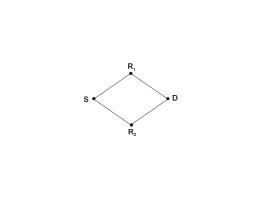
(a) Original network with multiple antenna nodes

(b) Equivalent network with single antenna nodes

Figure 5: Source and sink have $2$ antennas each, relays have $3$ each

It must be noted that even wireline networks can be converted into the above model of wireless networks. This can be done by adding as many number of small nodes in a super node as the number of edges emanating from or arriving at a node. Then, by making the coefficients of chosen edges to zero (or equivalently by removing corresponding edges from the representation), the broadcast and interference constraints can be nullified. Thus the class of wireline networks are naturally embedded in the class of wireless networks in the above representation.

III-B Min-cut equals Diversity

Theorem III.1

Consider a multi-terminal fading network with nodes having multiple antennas with edges connecting antennas on two different nodes having i.i.d. Rayleigh-fading coefficients. The maximum diversity achievable for any flow is equal to the min-cut between the source of the flow and the corresponding sink. Each flow can achieve its maximum diversity simultaneously.

Proof:

We first consider the case where there is only a single source-sink pair. We will handle the case of single and multiple-antenna nodes separately.

Case I: Network with single antenna nodes

Let the source be $S_{i}$ and sink be $D_{j}$. Let $\Lambda_{ij}$ denote the set of all cuts between $S_{i}$ and $D_{j}$.

From the cut-set upper bound on DMT (see Lemma II.1),

$$d(r) \leq \min_{\Omega\in\Lambda_{ij}}d_{\Omega}(r)$$

$$\Rightarrow d(0) \leq \min_{\Omega\in\Lambda_{ij}}d_{\Omega}(0)$$

$$=: \min_{\Omega\in\Lambda_{ij}}m_{\omega},$$

where $m_{\omega}$ is the number of edges crossing from the source side to the sink side in the cut $\omega$. So, now $d(0)\leq m$, where $m:=\min_{\omega}m_{\omega}$ is the min-cut.

It suffices to prove that a diversity order equal to $m$ is achievable. We know from Menger’s theorem in graph theory (see for eg.  [51]), that the number of edges in the min-cut is equal to the maximum number of edge-disjoint paths between source and the sink. Schedule the network in such a way that each edge in a given edge-disjoint path is activated one by one. The same is repeated for all the edge-disjoint paths. Let the number of edges in the $i$th edge-disjoint path be $n_{i}$. The $j$th edge in the the $i$th edge-disjoint path is denoted by $e_{ij}$ and the associated fading coefficient be $\mathbb{h}_{ij}$. Now define $\mathbb{h}_{i}:=\prod_{j=1}^{n_{i}}\mathbb{h}_{ij},i=1,2,...,m$. So the activation schedule will be as follows: $e_{11}$, $e_{12}$, $\cdots$, $e_{1(n_{1})}$, $e_{21}$, $\cdots$, $e_{2(n_{2})}$, $\cdots$, $e_{m1}$, $e_{m2}$, $\cdots$, $e_{m(n_{m})}$, where each edge is activated one at a time. The total number of time slots required for the protocol is $N:=\Sigma_{i=1}^{m}n_{i}$. This in effect creates a parallel channel between the source $S_{i}$ and destination $D_{j}$. The parallel channel contains $m$ links, with the fading coefficients $\mathbb{h}_{i}$ on the link $i$. With this protocol in place, the equivalent channel seen by a symbol is

$$\mathbb{H} = \left[\begin{array}[]{cccccc}\mathbb{h}_{1}&0&\ldots&&&0\\ 0&\mathbb{h}_{2}&0&&&0\\ \vdots&&\vdots&\ddots&&\\ 0&\ldots&\ldots&&&\mathbb{h}_{m}\end{array}\right].$$

This is a parallel channel with all the channels being independent of each other and the DMT of the channels being identical. Therefore we can use Corollary II.7 and obtain the DMT of the parallel channel as

$$d_{H}(r) = (m-r)^{+}.$$ (60)

This DMT can be achieved by using a DMT optimal parallel channel code.

The protocol utilizes $N$ time instants to induce this effective channel matrix, and therefore, the DMT of the protocol can be given in terms of the DMT of the channel matrix as

$$d(r) = d_{H}(Nr)$$ (61)

$$= (m-Nr)^{+}.$$ (62)

Hence the maximum achievable diversity is $m$.

Case II: Network with multiples antenna nodes

In the multiple antenna case, we pass on to the new representation described in Section III-A. We regard any link between a $n_{t}$ transmit and $n_{r}$ receive antenna as being composed of $n_{t}n_{r}$ links, with one link between each transmit and each receive antenna. Note that it is possible to selectively activate precisely one of the $n_{t}n_{r}$ Tx-antenna-Rx-antenna pairs by appropriately transmitting from just one antenna and listening at just one Rx antenna. As is to be expected, in this modified representation, a cut is defined as separating super-nodes into two sets since super-nodes represent distinct terminals. With this modification, the same strategy as in the single antenna case can then be applied to achieve a diversity equal to the min-cut in the network.

(a) Original network with multiple antenna nodes

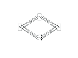
(b) Equivalent network with single antenna nodes

Figure 6: Illustration: $n_{S}=n_{D}=2,n_{1}=n_{2}=3$

Fig. 6 illustrates this conversion for the case of a single source $S$, two relays $R_{1}$ and $R_{2}$ and a sink $D$. Having converted the multiple antenna network into one with single antenna nodes, Case II follows from Case I. For the example shown in the figure, the min-cut and therefore the diversity is equal to $12$.

Thus the proof is complete for the single flow from $S_{i}$ to $D_{j}$.

When there are multiple flows in the network, we simply schedule the data of all the flows in a time-division manner. This will entail a rate loss - however, since we are interested only in the diversity, we can still achieve each flow’s maximum diversity simultaneously. ∎

III-C Maximum Multiplexing Gain equals Minimum Rank

In this section, we determine the maximum multiplexing gain (MMG) for multi-antenna ss-ss networks to be equal to the min-cut rank (which will be formally defined later). For ss-ss networks with single-antennas, the MMG is lesser than one, because the source has a single antenna and the cut with source at one side and the rest of the nodes on the other side will yield an upper bound on MMG as one. It is possible to attain the optimal MMG of $1$ by activating one path between the source to the destination either using amplify-and-forward or a decode-and-forward strategy. However, the MMG-optimal strategy becomes unclear when the number of antennas is greater than $1$.

We use results from a recent work on deterministic wireless networks [32] to arrive at strategies for achieving the maximum multiplexing gain of a fading network. The achievability strategies for deterministic wireless networks are lifted to fading networks using simple algebraic techniques. We begin with discussing a new representation for ss-ss networks, potentially having multiple antenna nodes, which will be used in this section.

III-C1 Linear Deterministic Wireless networks

In defining deterministic wireless networks, we follow [31]. Every terminal in the network is represented by a super-node and each node possesses $q$ small nodes associated with the super-node. All operations take place over a fixed finite field $\mathbb{F}_{p}$. There are edges drawn between small nodes of distinct super-nodes, representing communication channel between antennas of different terminals. Since we are dealing with deterministic wireless networks, we assume that the broadcast and interference constraints hold. In effect the vector ${\bf y}_{i}$ received by a super-node $i$ can be given in terms of the transmitted vectors ${\bf x}_{j}$ of various nodes by

$${\bf y_{i}}=\sum_{j\ \in\ \text{In}(i)}G_{ij}{\bf x_{j}},$$

where ${\bf y_{i}}$ and ${\bf x_{j}}$ are $q$ length column column vectors in $\mathbb{F}_{p}$, and $G_{ij}$ is a $m_{i}\times m_{j}$ transfer matrix between the super-node $i$ and super-node $j$, taking values in $\mathbb{F}_{p}$. Every cut $\omega$ in the deterministic network is associated with a channel matrix, which we will denote by ${G}_{\omega}$.

The network model of linear deterministic networks thus described has close similarities with representation of ss-ss fading networks described in Section III-A with the multiple antennas taking the place of small nodes in the case of fading networks. The difference between the two are only that deterministic network has noise-free links in comparison to the noisy links in the fading case, and that every edge coefficient is a finite field element in the deterministic network, in place of complex fading coefficient. In deterministic networks, each node transmits a $q$-tuple over the finite field. The theorem below from [31], computes the capacity of a ss-ss linear deterministic wireless network.

Theorem III.2

[31] Given a linear deterministic ss-ss wireless network over any finite field $\mathbb{F}_{p}$, $\forall\ \epsilon>0$, the capacity $C$ of such a relay network is given by,

$$C=\min_{\omega\ \in\ \Omega}\text{rank}(G_{\omega}),$$

where the capacity is specified in terms of the number of finite field symbols per unit time. A strategy utilizing only linear transformations over $\mathbb{F}_{p}$ at the relays is sufficient to achieve this capacity.

The capacity-achieving strategy in [31] utilizes matrix transformations of the input vector received over a period of $T$ time slots at each relay. This process continues for $L$ blocks, therefore the total number of time instants required for the scheme is $M:=LT$. The achievability shows the existence of relay matrices $A_{i}$ at each relay node $i\in|\mathcal{V}|$, where $\mathcal{V}$ is the set of vertices in the graph. $A_{i}$ is of size $qT\times qT$, and it represents the transformation between the received vector of size $qT$ to the vector of size $qT$ that is transmitted.

The multi-cast version of TheoremIII.2 is reproduced below:

Theorem III.3

[31] Given a linear deterministic single-source $D$-sink multi-cast wireless network, $\forall\ \epsilon>0$, the capacity $C$ of such a network is given by,

$$C=\min_{j=1,2,..,D}\ \min_{\omega\in\ \Omega_{j}}\text{rank}(G_{\omega}).$$

where $\Omega$ is the set of all cuts between the source and destination $j$. A strategy utilizing only linear transformations at the relays is sufficient to achieve this capacity.

III-C2 MMG of ss-ss networks

The main result of this section is given below.

Theorem III.4

Given a ss-ss multi-antenna wireless network, with Rayleigh fading coefficients, the MMG of the network is given by

$$D=\min_{\omega\ \in\ \Omega}\mathbb{R}\mathrm{ank}(\mathbb{H_{\omega}}).$$

An amplify-and-forward strategy utilizing only linear transformations at the relays (that do not depend on the channel realization) is sufficient to achieve this MMG.

Proof:

(Outline) The proof proceeds as follows:

1. First, a converse for the MMG is provided using simple cut-set bounds.

2. Then, we convert the fading network into a deterministic network with the property that the cut-set bound on MMG for the fading network is the same as the cut-set bound on the capacity of the deterministic network.

3. We then characterize the zero-error capacity of the linear deterministic wireless network.

4. Finally, we convert a capacity-achieving scheme for the deterministic network into a MMG-achieving scheme for the fading network, which matches the converse.

∎

The outline of the proof given above is detailed below. A converse on the degrees of freedom of a ss-ss fading network is immediate and is formalized in the following lemma.

Lemma III.5

Given a ss-ss fading network with i.i.d. Rayleigh fading coefficients, the MMG, $D$, is upper bounded by the MMG of every cut:

$$D \leq \min_{\omega\ \in\ \Lambda}\mathbb{R}\mathrm{ank}(\mathbb{H_{\omega}}),$$ (63)

where $\Lambda$ denotes the set of all cuts in the network, and $\mathbb{H_{\omega}}$ is the matrix corresponding to the cut $\omega\in\Lambda$.

Next we proceed to the achievability part of the proof. First, we convert the wireless fading network into a derived linear deterministic network. The construction of the derived deterministic network is described below. We will show that the zero-error capacity of this derived deterministic network is lower bounded by the upper-bound on the MMG of the fading network.

Let the number of edges in the fading network be $N$. Fading coefficients associated with edges of the network are denoted by $\mathbb{h}_{1},\mathbb{h}_{2},...,\mathbb{h}_{N}$. To construct the derived deterministic network, consider a deterministic network with the same topology as that of the original fading network. We take $q$, the vector length in the deterministic network to be equal to the maximum number of antennas of any node in the fading network. For nodes with number of antennas less than $q$, we leave the remaining nodes unconnected. We still need to decide the finite field size, $p$, and finite field coefficients on all edges to completely characterize the equivalent finite-field deterministic network. We shall denote these finite-field coefficients by $\xi_{i},\ i=1,2,\ldots,N$. We shall consider $\{\xi_{i}\}$ as indeterminates, before values are assigned to them.

For determining the field size $p$ and $\{\xi_{i},\ i=1,2,\ldots,N\}$, we will impose further conditions. In particular, we will ensure that the deterministic network will have at least the same capacity as the upper bound on MMG for the fading network. Due to the similarity between the expression for capacity in Theorem III.2 and MMG terms in Lemma III.5, above condition can be met by making sure that, cut-by-cut, the rank of the transfer matrix $(G_{\omega})$ in the deterministic network is at least as large as the structural rank of the transfer matrix $\mathbb{H}_{\omega}$, i.e., $\text{rank}(G_{\omega})\geq\mathbb{R}\mathrm{ank}(\mathbb{H}_{\omega})$.

Let us fix a cut $\omega$, and let $r_{\omega}:=\mathbb{R}\mathrm{ank}(\mathbb{H}_{\omega})$ be the structural rank of the transfer matrix of the cut in the fading network. Then, there exists a $r_{\omega}\times r_{\omega}$ sub-matrix (say $\mathbb{H}^{{}^{\prime}}_{\omega}$) of $\mathbb{H}_{\omega}$, which has structural rank $r_{\omega}$. Consider the same cut on the deterministic network and find the corresponding $r_{\omega}\times r_{\omega}$ sub-matrix $G^{{}^{\prime}}_{\omega}$ of the transfer matrix $G_{\omega}$. Now consider the determinant of the matrix $G^{{}^{\prime}}_{\omega}$. The determinant is a polynomial in several variables $\xi_{i},i=1,2,..,N$ with rational integer coefficients. Let us call this polynomial as $f_{\omega}(\xi_{1},\xi_{2},..,\xi_{N})$. This polynomial is not identically a zero polynomial over $\mathbb{Q}$. This is because if it had been, then the substitution of $\xi_{i}=h_{i}$ will also yields zero irrespective of the choice of $h_{i}$, making the determinant zero even for the gaussian case, leading to a contradiction. Therefore, $f_{\omega}$ is a non-zero polynomial. We also observe that the degree of $f_{\omega}$ in each of the variable $\xi_{i}$ is at most one. The lemma below, easily proved using elementary algebra, shows that it is possible to identify a finite field $\mathbb{F}_{p}$ and an allocation to $\{\xi_{i}\}$ with numbers from $\mathbb{F}_{p}$ such that $f_{\omega}$ does not vanish.

Lemma III.6

Given a polynomial $f(\xi_{1},\xi_{2},...,\xi_{N})$ with integer coefficients, which is not identically zero, there exists a prime field $\mathbb{F}_{p}$ with $p$ large enough, such that the polynomial evaluates to a non-zero value at least for one assignment of field values to the formal variables.

However we want ensure the above condition for every cut in the network. To do so, consider the polynomial

$$f(\xi_{1},\xi_{2},..,\xi_{N}):=\prod_{\omega\in\Omega}f_{\omega}(\xi_{1},\xi_{2},..,\xi_{N}).$$ (64)

Now, the polynomial $f$ is non-zero since it is a product of non-zero polynomials $f_{\omega}$ and the degree of $f$ in any of the variables is at-most $|\Omega|$. We want a field $\mathbb{F}_{p}$ and an assignment for $\xi_{i}$ from the field such that $f$ is nonzero. Using Lemma III.6, such an assignment exists. Let us choose that $p$ and the assignment that makes $f$ non-zero. Thus we have a deterministic wireless network whose capacity is guaranteed to be greater than or equal to the MMG upper bound, given in (63).

Next, we prove that the zero error capacity, $C_{ZE}$, of a linear deterministic network is equal to its $\epsilon$-error capacity.

Definition 4

[39] The zero error capacity of a channel is defined as the supremum of all achievable rates across the channels such that the probability of error is exactly zero.

Theorem III.7

The zero error capacity of a ss-ss deterministic wireless network is equal to

$$C_{ZE} = \min_{\omega\ \in\ \Omega}\mathrm{rank}(G_{\omega})$$

This capacity can be achieved using a linear code and linear transformations in all relays.

Proof:

We will prove this theorem using the $\epsilon$-error capacity result from Theorem III.2. Let the ss-ss deterministic network be composed of $M$ relay nodes. From the achievability result in the proof of Theorem III.2, given any $\epsilon>0$ and rate $r<C$, there exists a block length $T$, number of blocks $L$, set of linear transformations $A_{j},j=1,2,...,M$ of size $qT\times qT$ used by all relays and a code book $\mathcal{C}$ for the source, such that the average probability of error, $P_{e}$, is less than or equal to $\epsilon$. Each codeword $x_{i}\in\mathcal{C}$ is a $qT\times 1$ vector that specifies the entire transmission from the source. Let $x_{1},...,x_{|\mathcal{C}|}$ be the codewords.

Let us assume that the sink listens for $L^{{}^{\prime}}\geq L$ blocks in general to account for the presence of paths of unequal lengths in the network between source and sink, (for large $L$, we would have $\frac{L^{{}^{\prime}}}{L}\rightarrow 1$, so this does not affect rate calculations). Let $M:=LT$ and $M^{{}^{\prime}}:=L^{{}^{\prime}}T$. The transfer equation between the source and the destination vectors are specified by, $\mathbb{y}=G\mathbb{x}$ since all transformations in the network are linear. Here $G$ is a $qM^{{}^{\prime}}\times qM$ matrix, $\mathbb{x}$ is the $M$-length transmitted vector, and $\mathbb{y}$ is the $M^{{}^{\prime}}$-length received vector.

Given the transmitted vector $\mathbb{x}_{i}$ corresponding to a message $m_{i}$ at the source, the decoder either makes an error always or never makes an error. This is because the channel is a deterministic linear map, and error is only due to the fact that $x_{i}$ and $x_{j}$ are mapped to the same vector at the decoder. Let $P_{e}^{i}$ be the probability of error, conditioned on the fact that the $i$-th codeword, $\mathbb{x}_{i}$ is transmitted. Then $P_{e}^{i}\in\{0,1\}$ according to the argument above and the average codeword error probability

$$P_{e}=\frac{1}{|\mathcal{C}|}\sum_{i=1}^{|\mathcal{C}|}P_{e}^{i}\ \leq\ \epsilon \Rightarrow \sum_{i=1}^{|\mathcal{C}|}P_{e}^{i}\leq\epsilon|\mathcal{C}|.$$

This means that at least $(1-\epsilon)|\mathcal{C}|$ codewords have zero probability of error. Therefore if we choose only these $(1-\epsilon)|\mathcal{C}|$ codewords as an expurgated code $\mathcal{C}^{{}^{\prime}}$, then the code has zero probability of error under the same relay matrices and decoding rule. The rate of the code is however $\bar{r}=r-\frac{\log\{(1-\epsilon)^{-1}\}}{M}$. Let $\delta=\frac{\log\{(1-\epsilon)^{-1}\}}{M}$ be the rate loss and therefore, the expurgated code has negligible rate loss as $M$ becomes large. Now, we have established a zero error code of rate $r-\delta$. By choosing $r$ arbitrarily close to $C$ and $M$ large, we get $C_{ZE}=C$.

The code ${\cal C}$, as given in [31] is non-linear, and so is the case of ${\cal C}^{{}^{\prime}}$. However, we can obtain a linear code with zero probability of error. Since there exists a zero error code for rate $\bar{r}$ with block length $T$ and number of blocks $L$, it means that the transfer matrix $G$ between the source and the sink has rank at least $\bar{r}M$. Hence $G$ has a sub-matrix $G^{{}^{\prime}}$ of size $\bar{r}M\times\bar{r}M$, which is of full rank. By activating appropriate nodes, we can obtain the effective transfer matrix to be $G^{{}^{\prime}}$. In that case, a linear code of rate $\bar{r}$ which communicates only on the $\bar{r}M$ subspaces can be used to achieve zero error. ∎

Thus, for a given fading network, we have constructed an equivalent deterministic network. In the equivalent network, we also have a zero-error achievable rate $\bar{r}$ using a linear code of block length $T$ and $L$ blocks with linear strategies at the relays. This achievable rate is related to the MMG of the original fading network as follows:

$$\bar{r}+\delta = C_{ZE}$$

$$= \min_{\omega\ \in\ \Omega}\mathrm{rank}(G_{\omega})$$

$$\geq \min_{\omega\ \in\ \Omega}\mathbb{R}\mathrm{ank}(\mathbb{H_{\omega}})$$

Further, the positive constant $\delta$ can be made as small as possible as we wish by increasing the block length $T$. Now, when we use the zero-error scheme detailed above, the transfer matrix $G$ of size $qM\times qM$ between the input and the output vectors $\mathbb{x}$ and $\mathbb{y}$ is at least of rank $\bar{r}M\approx CM$.

Finally, we lift the achievability strategy of zero-error capacity in the equivalent deterministic networks to arrive at an achievable strategy for MMG in corresponding fading network.

In the reduced deterministic network of a fading network, to achieve the zero-error capacity, the relays perform matrix operations $A_{i}$ on received vectors for $T$ time durations. Since each received vector is of size $q$, the matrix $A_{i}$ is of size $qT\times qT$. Now we use the same strategy for the fading network, i.e., all relays use the same matrices $A_{i}$, that are obtained via the zero-error strategy in the reduced deterministic network. Though the entries of $A_{i}$ belong to $\mathbb{F}_{p}$, they can be treated as integers by identifying the elements of $\mathbb{F}_{p}$ with the integers $0,1,,...,(p-1)$. Therefore the matrices $A_{i}$ can also be interpreted as matrices over $\mathbb{C}$. By using linear maps $A_{i}$ at relays in the fading network, we get an induced channel matrix ${\bf H}$, and effective channel would be of the form, ${\bf y}\ =\ {\bf H}{\bf x}+{\bf w}$. As is shown in Theorem II.11, MMG offered by this channel is equal to $\mathbb{R}\mathrm{ank}(\mathbb{H})$. We shall prove that MMG offered by this induced channel is greater than or equal to $\bar{r}M$, i.e., to show that $\mathbb{R}\mathrm{ank}(\mathbb{H})\geq\bar{r}M$. That is equivalent to show that there exists an assignment of $\mathbb{h}_{i}=h_{i}$ in the fading network such that $\text{rank}(H)\geq\bar{r}M$.

In the proof of Theorem III.7, we restricted the operation of the derived deterministic network to create a transfer matrix $G$ of size $qM\times qM$ with rank greater than or equal to $\bar{r}M$. Now we have a similar transfer matrix $\mathbb{H}$ in the fading network. If we assign the underlying random variables $\mathbb{h}_{i}$ to be equal to $\xi_{i}$, again by identifying the elements of $\mathbb{F}_{p}$ with the integers $0,1,,...,(p-1)$, we have an assignment of $\mathbb{H}$ that has rank at least $\bar{r}M$. Since the strucutral rank is the maximum possible rank under any assignment, we get that,

$$\mathbb{R}\text{ank}(\mathbb{H}) \geq \text{rank}(G)\geq\bar{r}M.$$

The induced channel therefore has a MMG equal to $\bar{r}M$ by Theorem II.11. Since the network is operated for $M=LT$ time slots in order to obtain a MMG greater than or equal to $\bar{r}M$, the MMG of the network per time slot is greater than or equal to $\bar{r}$. By increasing the block length $T$ and the number of blocks $L$, the achievable MMG can be made arbitrarily close to $C_{ZE}$. Thus the upper bound given in Lemma III.5 is achieved, and hence MMG of ss-ss fading network is given by

$$D = \min_{\{\omega\ \in\ \Lambda\}}\mathbb{R}\mathrm{ank}(\mathbb{H}_{\Lambda}).$$

III-D MMG for Multi-casting

In this section, we extend the result on MMG to the multi-casting scenario.

Theorem III.8

Given a single-source $D$-sink multi-cast gaussian wireless network, with Rayleigh fading coefficients, the MMG of the network is given by

$$D=\min_{\{j=1,2,...,D\}}\ \min_{\omega\ \in\ \Omega_{j}}\mathbb{R}\mathrm{ank}(\mathbb{H}_{\omega}).$$ (65)

An amplify-and-forward strategy utilizing only linear transformations at the relays is sufficient to achieve this MMG.

Proof:

The proof uses Theorem III.3, goes in the similar lines of that of Theorem III.4 and is omitted here for brevity. ∎

IV DMT Bounds for Single Antenna Relay Networks

In this section, we consider ss-ss networks equipped with full-duplex single-antenna nodes. We provide a lower bound to the DMT of such a network by exploiting Menger’s theorem.

Definition 5

Consider a network $N$ and a path $P$ from source to sink. This path $P$ is said to have a shortcut if there is a single edge in $N$ connecting two non-consecutive nodes in $P$.

Theorem IV.1

Consider a ss-ss full-duplex network with single antenna nodes. Let the min-cut of the network be $M$. Let the network satisfy either of the two conditions below:

1. The network has no directed cycles, or

2. There exist a set of $M$ edge-disjoint paths between source and sink such that none of the $M$ paths have shortcuts.

Then, a linear DMT $d(r)=M(1-r)^{+}$ between a maximum multiplexing gain of $1$ and maximum diversity $M$ is achievable.

Proof:

Given that the network has min-cut $M$, there are $M$ edge-disjoint paths from source to sink by Menger’s theorem [51]. Let us label the edge-disjoint paths $e_{1},e_{2},...,e_{M}$. Let the product of the fading coefficients along the path $e_{i}$ be $g_{i}$. Let $D_{i}$ be the delay of each path. Let $D=\max D_{i}$. We add delay $D-D_{i}$ to the path $e_{i}$ such that all paths now are of equal delay. We activate the edges as follows:

1. Activate all edges in the edge-disjoint path $e_{1}$ simultaneously for a period $T$, where $T>>D$. The source, on the first $T-D$ activations, will transmit $(T-D)$ coded information symbols, followed by a sequence of $D$ zero symbols. The reason for this will become clear shortly. The net effect will be to create a $((T-D)\times(T-D)$ transfer matrix ${\bf H}_{1}$ from the $(T-D)$ source symbols to the last $(T-D)$ symbols received by the destination (the first $D$ symbols received by the destination are all zero).

   The matrix ${\bf H}_{1}$ will be either upper-triangular or lower-triangular, with the elements along the diagonal all equal to the path gain ${\bf g}_{1}$ on path $e_{1}$, according to whether the condition $1$ or condition $2$ of the theorem is satified. First, we explain the case when the graph has no directed cycles. In this case, off-diagonal terms above the diagonal can arise due to the presence of short-cuts. However, off-diagonal terms below the diagonal would constitute a directed cycle and will thus not appear. Therefore the matrix will be upper-triangular in this case. Next, for the case when the graph has no shortcuts, off-diagonal terms below the diagonal can arise due to the presence of cycles in the graph. However, no terms above the diagonal will be present because of the presumed absence of shortcuts. Thus the induced matrix will be lower-triangular in structure.

2. Repeat Step 1 for all edge-disjoint paths $e_{2},...,e_{M}$. The net transfer matrix ${\bf H}$ will be block diagonal of the form

   $${\bf H} = \left[\begin{array}[]{cccc}{\bf H}_{1}&&&\\ &{\bf H}_{2}&&\\ &&\ddots&\\ &&&{\bf H}_{M}\end{array}\right].$$ (70)

   composed of $M$ blocks along the diagonal, one corresponding to each path, and either all of them are upper triangular or all are lower triangular by the argument above.

Now, if $d(r)$ is the DMT of the network operating under the protocol given above, then

$$d(r) = d_{H}(MTr),$$ (71)

since $MT$ time instants were used up by the protocol in order to obtain the indcued channel matrix $\mathbb{H}$. We next proceed to lower bound $d_{H}(r)$. By Theorem II.12, we have the lower bound

$$d_{H}(r) \geq d_{H^{(0)}}(r)$$ (72)

where ${\bf H}^{(0)}$ is the matrix corresponding to the diagonal terms in ${\bf H}$. Next, we observe that ${\bf H}^{(0)}$ corresponds to a parallel channel with $M$ fading coefficients ${\bf g}_{1},{\bf g}_{2},\cdots,{\bf g}_{M}$, each of them repeated $T-D$ times. We can compute the DMT of this parallel channel using Lemma II.8. Thus we get,

$$d_{H^{(0)}}(r) = M\left(1-\frac{r}{M(T-D)}\right)^{+}$$ (73)

$$\Rightarrow d(r) = d_{H}(MTr)\geq d_{H^{(0)}}(MTr)$$ (74)

$$d(r) = M\left(1-\frac{MTr}{M(T-D)}\right)^{+}.$$ (75)

For $T$ tending to $\infty$, we get $d(r)\geq M(1-r)^{+}$. ∎

Appendix A Proof of Lemma II.2

Let the multinomial $f$ be written as a sum of $S$ monomials $f(X_{1},X_{2},...,X_{M}):=\sum_{i=1}^{S}c_{i}f_{i}(X_{1},X_{2},...,X_{M}$), where for every $i$, $c_{i}$ is a constant and $f_{i}$ is a monomial, i.e., is comprised only of product of powers of $X_{i}$. Then for every assignment, $X_{i}=h_{i}$,

$$|f(h_{1},h_{2},...,h_{M})|\leq\sum_{i}|c_{i}||f_{i}(h_{1},h_{2},...,h_{M})|.$$

Now we have,

$$\Pr\{|f(\mathbb{h}_{1},\mathbb{h}_{2},...,\mathbb{h}_{M})|^{2}>k\}$$

$$= \Pr\{|f(\mathbb{h}_{1},\mathbb{h}_{2},...,\mathbb{h}_{M})|>k^{\frac{1}{2}}\}$$

$$\leq \Pr\{\sum_{i}|c_{i}||f_{i}(\mathbb{h}_{1},\mathbb{h}_{2},...,\mathbb{h}_{M})|>k^{\frac{1}{2}}\}$$

$$\leq \Pr\left\{\bigcup_{i}\left(|c_{i}||f_{i}(\mathbb{h}_{1},\mathbb{h}_{2},...,\mathbb{h}_{M})|>\frac{k^{\frac{1}{2}}}{S}\right)\right\}$$

$$\leq \sum_{i}\Pr\left\{|c_{i}|^{2}|f_{i}(\mathbb{h}_{1},\mathbb{h}_{2},...,\mathbb{h}_{M})|^{2}>\frac{k}{S^{2}}\right\}$$

$$\leq \sum_{i}\Pr\left\{|f_{i}(\mathbb{h}_{1},\mathbb{h}_{2},...,\mathbb{h}_{M})|^{2}>\frac{k}{c_{max}S^{2}}\right\},$$ (77)

where $c_{max}$ is the maximum over all $\{|c_{i}|^{2}\}$. Now $|f_{i}(h_{1},h_{2},...,h_{M})|^{2}$ is a monomial in $|h_{i}|^{2}$ as well. Define, $\mathbb{u}_{j}:=|\mathbb{h}_{j}|^{2}$. Then $\mathbb{u}_{j}$ is the squared norm of a $\mathbb{C}\mathcal{N}(0,1)$ random variable $\mathbb{h}_{j}$, and therefore has an exponential distribution. We will regard $|f_{i}(\mathbb{h}_{1},\mathbb{h}_{2},...,\mathbb{h}_{M})|^{2}$ as a monomial $g_{i}(\mathbb{u}_{1},\mathbb{u}_{2},...,\mathbb{u}_{M})$ in $\{\mathbb{u}_{j}\}$. Thus

$$g_{i}(\mathbb{u}_{1},\mathbb{u}_{2},\ldots,\mathbb{u}_{M})=\prod_{j=1}^{M}{\mathbb{u}_{j}}^{a_{ij}},$$

where $0\leq a_{ij}\leq D$ is an integer, where $D$ is the maximum degree of any of the monomials $g_{i}$ in any of the variables $\mathbb{h}_{i}$.

Now gathering a single term in the summation in RHS of (77), we have,

$$\Pr\left\{|f_{i}(\mathbb{h}_{1},\mathbb{h}_{2},...,\mathbb{h}_{M})|^{2}>\frac{k}{c_{max}S^{2}}\right\}$$

$$= \Pr\left\{g_{i}(\mathbb{u}_{1},\mathbb{u}_{2},\ldots,\mathbb{u}_{M})>\frac{k}{c_{max}S^{2}}\right\}$$

$$\leq \Pr\left\{\bigcup_{j}\left({\mathbb{u}_{j}}^{a_{ij}}>\left(\frac{k}{c_{max}S^{2}}\right)^{\frac{1}{M}}\right)\right\}$$

$$\leq \sum_{j}\Pr\left\{{\mathbb{u}_{j}}^{a_{ij}}>\left(\frac{k}{c_{max}S^{2}}\right)^{\frac{1}{M}}\right\}$$

$$= \sum_{j}\Pr\left\{{\mathbb{u}_{j}}>\left(\frac{k}{c_{max}S^{2}}\right)^{\frac{1}{Ma_{ij}}}\right\}$$

$$\leq \sum_{j}\Pr\left\{{\mathbb{u}_{j}}>\left(\frac{k}{c_{max}S^{2}}\right)^{\frac{1}{MD}}\right\}$$

$$= M\ \Pr\left\{{\mathbb{u}_{j}}>\left(\frac{k}{c_{max}S^{2}}\right)^{\frac{1}{MD}}\right\}$$

$$= M\ \exp\left(-\left(\frac{k}{c_{max}S^{2}}\right)^{\frac{1}{MD}}\right).$$ (79)

Equation (A) follows if

$${k} \geq {c_{max}S^{2}}.$$

We get this condition by setting $\delta:={c_{max}S^{2}}>0$, since by the hypothesis of the lemma, we have $k\geq\delta$.

Combining (77) and (79), we get, for $k\geq\delta$,

$$\Pr\{|f(\mathbb{h}_{1},\mathbb{h}_{2},...,\mathbb{h}_{M})|^{2}>k\}$$

$$\leq MS\ \exp\left(-\left(\frac{k}{c_{max}S^{2}}\right)^{\frac{1}{MD}}\right)$$

$$= A\ \exp\left(-Bk^{\frac{1}{d}}\right)\$$

where $A:=MS$, $B:=\left({\frac{1}{c_{max}S^{2}}}\right)^{\frac{1}{MD}}$, $\delta={c_{max}S^{2}}$ and $d:=MD$.

Appendix B Proof of Theorem II.3

$$Pr(\log\det(I+\rho\mathbb{H}\mathbb{H}^{\dagger}\Sigma^{-1})\leq r\log\rho)$$

$$\doteq Pr(\log\det(I+\rho\mathbb{H}\mathbb{H}^{\dagger})\leq r\log\rho).$$

Let the correlation matrix of the noise vector be denoted by $\mathbb{\Sigma}$. The noise covariance matrix $\mathbb{\Sigma}$ depends on the channel realization and is therefore a random matrix, given by,

$$\mathbb{\Sigma} = \mathbb{E}_{\bf z}[{\bf z}{{\bf z}^{\dagger}}]$$ (80)

$$= I+\sum_{i=1}^{M}\mathbb{G}_{i}\mathbb{G}_{i}^{\dagger}.$$

Let $\lambda_{i}(A)$, $\lambda_{max}(A)$ and $\lambda_{min}(A)$ denote the $i^{\text{th}}$ largest, maximum and minimum eigenvalues of a positive semi-definite matrix $A$. If the context is clear, we may avoid specifying the matrix, and just use $\lambda_{i}$, $\lambda_{max}$ and $\lambda_{min}$ respectively.

To prove the lemma, we will use the Amir-Moez bound on the eigen values of the product of Hermitian, positive-definite matrices [52]. By this bound, for any two positive definite $n\times n$ Hermitian matrices $A,B$:

$$\lambda_{i}(A)\lambda_{min}(B)\leq \lambda_{i}(AB) \leq\lambda_{i}(A)\lambda_{max}(B).$$

So we get,

$$\det(I+\rho AB) = \prod_{i}(1+\rho\lambda_{i}({AB}))$$

$$\leq \prod_{i}(1+\rho\lambda_{i}(A)\lambda_{{\max}}(B))$$

$$= \det(I+\rho\lambda_{{\max}}(B)A).$$

Similarly,

$$\det(I+\rho AB) \geq \det(I+\rho\lambda_{\min}(B)A).$$

Therefore, for any two positive definite $n\times n$ Hermitian matrices $A,B$,

$$\det(I+\rho\lambda_{\min}(B)A)$$

$$\leq\det(I+\rho AB)\leq\ \det(I+\rho\lambda_{\max}(B)A).$$ (81)

Applying (81) to $A=\mathbb{H}\mathbb{H}^{\dagger}$ and $B=\mathbb{\Sigma}^{-1}$, we get

$$\Rightarrow\hbox to0.0pt{$\displaystyle\det(I+\rho{\bf H}{\bf H}^{\dagger}\lambda_{min}(\mathbb{\Sigma}^{-1}))$\hss}$$ (83)

$$\leq\det(I+\rho{\bf H}{\bf H}^{\dagger}\mathbb{\Sigma}^{-1})$$

$$\leq\det(I+\rho{\bf H}{\bf H}^{\dagger}\lambda_{max}(\mathbb{\Sigma}^{-1})).$$

Continuing from (83) and (83), we have

$$\Pr\{\log(\det(I+\rho{H}{H}^{\dagger}\lambda_{min}(\mathbb{\Sigma}^{-1})))<r\log\rho\}$$

$$\geq\Pr\{\log\det(I+\rho{H}{H}^{\dagger}\mathbb{\Sigma}^{-1})<r\log\rho\}$$

$$\geq\Pr\{\log(\det(I+\rho{H}{H}^{\dagger}\lambda_{max}(\mathbb{\Sigma}^{-1})))<r\log\rho\}.$$

In the following, we will prove that both the bounds coincide as $\rho$ $\rightarrow$ $\infty$. We begin with the bounds on $\lambda_{min}(\mathbb{\Sigma})$ and $\lambda_{max}(\mathbb{\Sigma})$. In order to show that the lower and the upper bounds on the expression converge to the value $\Pr\{\log(\det(I+\rho{H}{H}^{\dagger}))<r\log\rho\}$, we need to provide a lower bound for each $\lambda_{i}(\mathbb{\Sigma})$. Let $e_{i}$ be the eigen vector corresponding to $\lambda_{i}({\Sigma})$ for every realization $\Sigma$ of $\mathbb{\Sigma}$. Then,

$${\lambda_{i}(\Sigma)}\parallel{e_{i}}\parallel^{2} = {e_{i}}^{\dagger}\Sigma{e_{i}}$$

$$= {e_{i}}^{\dagger}\left(I+\sum_{i=1}^{M}\mathbb{G}_{i}\mathbb{G}_{i}^{\dagger}\right){e_{i}}$$

$$= \parallel{e_{i}}\parallel^{2}+{e_{i}}^{\dagger}{\left(\sum_{i=1}^{M}\mathbb{G}_{i}\mathbb{G}_{i}^{\dagger}\right)}{e_{i}}$$

$$\geq \parallel{e_{i}}\parallel^{2}$$

$$\Rightarrow{\lambda_{i}(\bf\Sigma)} \geq 1\ \ \forall i$$

$$\Rightarrow\lambda_{min}(\bf\Sigma) \geq 1$$ (85)

$$\Rightarrow\lambda_{max}(\bf\Sigma^{-1}) \leq 1$$

Hence, $$\Pr\{\log\det(I+\rho\mathbb{H}\mathbb{H}^{\dagger}{\bf\Sigma}^{-1})<r\log\rho\}$$ (86)

$$\geq \Pr\{\log\det(I+\rho\mathbb{H}\mathbb{H}^{\dagger}\lambda_{max}({\bf\Sigma}^{-1}))<r\log\rho\}$$

$$\geq \Pr\{\log\det(I+\rho\mathbb{H}\mathbb{H}^{\dagger})<r\log\rho\}$$

$$\doteq \rho^{d_{out}(r)}.$$ (87)

Now we proceed to get an upper bound on $\lambda_{max}(\mathbb{\Sigma})$:

$$\lambda_{max}({\bf\Sigma}) = \lambda_{max}(I+\sum_{i=1}^{M}{\bf G}_{i}{\bf G}_{i}^{\dagger})$$

$$= 1+\lambda_{max}(\sum_{i=1}^{M}\mathbb{G}_{i}\mathbb{G}_{i}^{\dagger})$$

i.e.,

$$\lambda_{max}({\bf\Sigma}) \leq 1+\text{Tr}\ (\sum_{i=1}^{M}\mathbb{G}_{i}\mathbb{G}_{i}^{\dagger})$$ (88)

$$= 1+\sum_{i=1}^{M}\text{Tr}\ (\mathbb{G}_{i}\mathbb{G}_{i}^{\dagger})$$

$$= 1+\sum_{i=1}^{M}{||\mathbb{G}_{i}||^{2}}_{F}$$

$$= 1+\sum_{i=1}^{M}\sum_{j=1}^{N^{2}}|f_{ij}|^{2},$$

where $f_{ij}$ represents a polynomial entry of the matrix $G_{i}$. Let $\mathbb{x}_{1},\mathbb{x}_{2},...,\mathbb{x}_{2L}$ denote in some order, the real and imaginary parts of $\mathbb{h}_{1},\mathbb{h}_{2},...,\mathbb{h}_{L}$. Then, the right hand side in (88) is a polynomial in the variables, $\mathbb{x}_{i},i=1,2,...,2L$.

This leads to the following inequality,

$$\lambda_{max}(\mathbb{\Sigma})\leq g(\mathbb{x}_{1},\mathbb{x}_{2},\ldots,\mathbb{x}_{2L})+1,$$ (89)

where $g(x_{1},x_{2},\ldots,x_{2L})$ is a polynomial without constant term in the variables $\{x_{i}\}$. Let us invoke Lemma II.2 for the polynomial $g$ which does not possess any constant term. The lemma is valid for all $k\geq\delta$, where $\delta$ depends on $g$. Let us choose $\rho_{0}$ such that $\rho_{0}^{\epsilon}-1\geq\delta$ and therefore $\forall\rho>\rho_{0}$, we have that $\rho^{\epsilon}-1\geq\delta$. Now, $\forall\rho>\rho_{0}$, we can invoke Lemma II.2 and get,

$$\Pr\{\lambda_{max}(\mathbb{\Sigma})>\rho^{\epsilon}\} \leq \Pr\{g(\mathbb{x}_{1},\mathbb{x}_{2},\ldots,\mathbb{x}_{S})>{\rho}^{\epsilon}-1\}$$ (90)

$$\leq A\exp(-B{(\rho^{\epsilon}-1)}^{\frac{1}{d}}),$$

for some constants $A$, $B$, $d>0$.

Let $\mathcal{H}$ denote the set of all the fading coefficients in the network, and let $\hbar\in\mathcal{H}$ denote a realization of the fading coefficients. Thus $\hbar$ will be a vector specifying $h_{i},i=1,2,...,L$. Clearly, once a $\hbar$ is given, the values of the matrices $H$ and $G_{i}$ are all well defined, since all of them depend only on $h_{i}$.

Let ${A}=\{\hbar\in\mathcal{H}\mid\log\det(I+{\rho}HH^{\dagger}\Sigma^{-1})<{\rho}^{r}\}$ and $B=\{\hbar\in\mathcal{H}\mid\lambda_{max}(\Sigma)>{\rho}^{\epsilon}\}$ be two events. Then,

$$\Pr(A) = \Pr(A\cap B^{c})+\Pr(A\cap B)$$ (91)

$$\leq \Pr(A\cap B^{c})+\Pr(B)$$

$$\dot{\leq} \Pr(A\cap B^{c})+A\exp(-B{(\rho^{\epsilon}-1)}^{\frac{1}{d}})$$

$$\text{Now, }A = \{\hbar\in\mathcal{H}\mid\log\det(I+{\rho}HH^{\dagger}\Sigma^{-1})<{\rho}^{r}\}$$

$$\subset \{\hbar\in\mathcal{H}\mid\log\det(I+{\rho}HH^{\dagger}\lambda_{min}(\Sigma^{-1}))<{\rho}^{r}\}$$

$$= \{\hbar\in\mathcal{H}\mid\log\det(I+{\rho}HH^{\dagger}{(\lambda_{max}(\Sigma))}^{-1})<{\rho}^{r}\}$$

$$A\cap B^{c} \subset \{\hbar\in\mathcal{H}\mid\log\det(I+{\rho}^{1-\epsilon}HH^{\dagger})<{\rho}^{r}\}.$$ (92)

Substituting (92) and (90) in (91), taking logarithms and dividing by $\log\rho$ on both sides, we have,

$$\frac{\log\Pr(A)}{\log\rho}$$ (93)

$$\leq \frac{\log[\Pr(A\cap B^{c})+\Pr(B)]}{\log\rho}$$

$$\dot{\leq} \frac{1}{\log\rho}\ .\ \log\ [\ \Pr\{\hbar\in\mathcal{H}\mid\log\det(I+{\rho}^{1-\epsilon}HH^{\dagger})<{\rho}^{r}\}$$

$$\ \ \ \ \ \ \ \ \ \ \ \ \ \ \ \ +\ \ A\exp(-B{(\rho^{\epsilon}-1)}^{\frac{1}{d}})\ ].$$

$$\lim_{\rho\rightarrow\infty}\frac{\log\Pr(A)}{\log\rho}$$

$$\dot{\leq} \lim_{\rho\rightarrow\infty}\frac{\log[\Pr\{\hbar\in\mathcal{H}\mid\log\det(I+{\rho}^{1-\epsilon}HH^{\dagger})<{\rho}^{r}\}]}{\log\rho}.$$

The last equation follows from (93), since the first term in the RHS of (93) varies inversely with an exponent of $\rho$ whereas the second term is exponential in $\rho$, and therefore the sum is dominated by the first term. After making the variable change, $\rho^{{}^{\prime}}=\rho^{1-\epsilon}$ and replacing $\rho$ by $\rho^{{}^{\prime}}$, we get

$$\Rightarrow\lim_{\rho\rightarrow\infty}\frac{\log\Pr\{\log\det(I+{\rho}\mathbb{H}\mathbb{H}^{\dagger}\mathbb{\Sigma}^{-1})<{\rho}^{r}\}}{\log\rho}$$ (94)

$$\dot{\leq} (1-\epsilon)$$

$$\lim_{\rho\rightarrow\infty}\frac{\log\Pr\{\log\det(I+{\rho}\mathbb{H}\mathbb{H}^{\dagger})<{\rho}^{(\frac{r}{1-\epsilon})}\}}{\log\rho}$$

$$\doteq (1-\epsilon)\rho^{d_{out}\left(\frac{r}{1-\epsilon}\right)}.$$

In (94), $\epsilon$ is arbitrary, and we let it tend to zero. Hence, by (94) and (87), the exponents for both the bounds in (LABEL:eq:outage_bound) coincide and we obtain,

$$\Pr\{\log\det(I+\rho\mathbb{H}\mathbb{H}^{\dagger}\Sigma^{-1})<r\log\rho\}$$

$$\doteq \Pr\{\log\det(I+\rho\mathbb{H}\mathbb{H}^{\dagger})<r\log\rho\}.$$

This proves the assertion of the theorem.

Appendix C Proof of Lemma II.9

Consider any two intervals $R_{1},R_{2}\in{\cal R}$. If we are not able to find two such intervals, then clearly $L\leq 1$, and we are done. Let $R_{1}=[a,b]$ and $R_{2}=[c,d]$, and without loss of generality assume that $a<b<c<d$, since they are, by hypothesis, disjoint. First, we claim that there exists a point $b\leq x_{0}\leq c$, such that either $p^{\prime}(x_{0})=0$, or $p^{\prime\prime}(x_{0})=0$. We now proceed to prove this claim.

Clearly, either of the two conditions (10) or (11) is violated just to the right of the point $x=b$, else, the interval would extend beyond $b$. We consider two cases.

Case 1: $|p(b)|\geq k$.

Condition (10) is violated in the region in the immediate right of the interval $[a,b]$. This implies that the absolute value of the evaluation of polynomial function, $|p(x)|$, has to be greater than $k$ in the beginning of the interval $[b,c]$. Also, we know that within $[a,b]$ and $[c,d]$, $|p(x)|$ is strictly less than $k$. This can happen in two ways, as shown in Fig. 7 (the other possibility is that the polynomial can be the negative of that shown in the figure, in which case the same argument holds). In either of these ways, the function has to go through $-k$ value twice in $[b,c]$. Therefore, by Rolle’s theorem, $p^{\prime}(x_{0})=0$, for some $b\leq x_{0}\leq c$.

(a) Case 1(a)

(b) Case 1(b)

Figure 7: Condition (10) is violated in $[b,c]$

(a) Case 2(a)

(b) Case 2(b)

Figure 8: Condition (11) is violated in $[b,c]$.

Case 2: Condition (11) is violated at the end of interval $[a,b]$

This implies that the absolute value of the evaluation of the derivative of $p(x)$, i.e.,$|p^{\prime}(x)|$, diminishes below $m$ in the beginning of the interval $[b,c]$. Also, we know that within $[a,b]$ and $[c,d]$, $|p^{\prime}(x)|$ is greater than or equal to $m$. This can happen only in two ways, as shown in Fig. 8. In the first case, $p^{\prime}(x_{0})=0$, for some $b\leq x_{0}\leq c$. In the second case, the function $p^{\prime}(x)$ takes the same value $+m$ twice in $[b,c]$, and hence by Rolle’s theorem, $p^{\prime\prime}(x_{0})=0$, for some $b\leq x_{0}\leq c$.

By the above claim, for any two arbitrary intervals in ${\cal R}$, there exists real root of $p^{\prime}(x)$ or $p^{\prime\prime}(x)$ between those two intervals. Since the number of roots of a polynomial is bounded by its degree, there will be only finitely many such intervals. In particular, the number of intervals $L$ is bounded by $2d$, which is an upper bound on the total number of zeros of $p(x)$ and $p^{{}^{\prime}}(x)$.

Appendix D Proof of Lemma II.10

For any polynomial $f$ in several gaussian random variables, we have that

$$\Pr\{f(\mathbb{x}_{1},\mathbb{x}_{2},...,\mathbb{x}_{N})\neq 0\} = 1.$$

This follows since letting

$$\underline{y} = (x_{1},x_{2},\cdots,x_{N-1})$$

$$S = \{x_{N}\mid f(x_{1},x_{2},\cdots,x_{N})=0\},$$

we see that

$$\Pr\{f(\mathbb{x}_{1},\mathbb{x}_{2},...,\mathbb{x}_{N})=0\} =$$

$$\int_{-\infty}^{\infty}\cdots\int_{-\infty}^{\infty}f(\underline{y})\int_{x_{N}\in S}f(x_{N}/\underline{y})dx_{N}d\underline{y} = 0,$$

because the innermost integral equals zero as $S$ is finite given a particular assignment of y, i.e.,

$$\int_{x_{N}\in S}f(x_{N}/\underline{y})dx_{N}\ =\ 0.$$ (95)

Let $\mathbb{x}:=\{\mathbb{x}_{1},\mathbb{x}_{2},...,\mathbb{x}_{N}\}$. Let us define an indicator function $I_{\delta}(\mathbb{x})$ as follows:

$$I_{\delta}(\mathbb{x}) := \left\{\begin{array}[]{ccc}1,&&\ |f(\mathbb{x}_{1},\mathbb{x}_{2},...,\mathbb{x}_{N})|<\delta\\ 0,&&\ \text{else}\\ \end{array}\right\}.$$

Then

$$\Pr\{|f(\mathbb{x}_{1},\mathbb{x}_{2},...,\mathbb{x}_{N})|^{2}<\delta\}$$

$$= \mathbb{E}_{\mathbb{x}}\ I_{k}(\mathbb{x})$$

$$= \mathbb{E}_{\mathbb{x}_{1},\mathbb{x}_{2},...,\mathbb{x}_{N-1}}\ \mathbb{E}_{\mathbb{x}_{N}}\{I_{k}(\mathbb{x})\ |\ \mathbb{x}_{1}^{N-1}\}$$

$$= \mathbb{E}_{\mathbb{x}_{1},\mathbb{x}_{2},...,\mathbb{x}_{N-1}}\ \Pr\ \{|f({x}_{1},{x}_{2},...,{x}_{N-1},\mathbb{x}_{N})|^{2}<\delta\}.$$

Let $f(\mathbb{x_{N}}):=f({x}_{1},{x}_{2},...,{x}_{N-1},\mathbb{x}_{N})$, where the dependence of $f$ on the first $N-1$ variables is made implicit. Let

$$f(\mathbb{x}_{N})=\sum_{k=0}^{d_{N}}b_{k}\mathbb{x}_{N}^{k},$$

where $d_{N}$ is the degree of the polynomial $f$ in the variable $x_{N}$. Since $b_{d_{N}}$ is a polynomial in the variables $x_{1}^{N-1}$, it follows from the lemma above that with probability one, $b_{d_{N}}\neq 0$.

Let

$$g(x_{N})=\frac{\partial f(x_{N})}{\partial x_{N}}$$

be the partial derivative of $f(x_{N})$ with respect to $x_{N}$. Then we can write

$$\Pr\ \{|f({x}_{1},{x}_{2},...,{x}_{N-1},\mathbb{x}_{N})|<\delta\}$$ (100)

$$= \Pr\ \{|f(\mathbb{x}_{N})|<\delta,|g(\mathbb{x}_{N})|\geq\delta^{1/2}\}$$

$$+\Pr\ \{|f(\mathbb{x}_{N})|<\delta,|g(\mathbb{x}_{N})|<\delta^{1/2}\}$$

$$\leq \Pr\ \{|f(\mathbb{x}_{N})|<\delta,|g(\mathbb{x}_{N})|\geq\delta^{1/2}\}$$

$$+\Pr\ \{|g(\mathbb{x}_{N})|<\delta^{1/2}\}.$$

Figure 9: f(x) in a region $R_{i}$

Let us consider the first term on the RHS. The region ${\cal R}:=\{|f({x}_{N})|<\delta,|g({x}_{N})|\geq\delta^{1/2}\}$ is described by two conditions $|f({x}_{N})|<\delta$ and $|g({x}_{N})|\geq\delta^{1/2}$. It is shown in Lemma II.9 that the set of all values of $x_{N}$ satisfying both conditions can be expressed as the union of $L$ pairwise-disjoint intervals $R_{i},i=1,2,...,L$ with $L<2d_{N}$. Now $\Pr(x_{N}\in R)=\sum_{i=1}^{L}\Pr(\mathbb{x}_{N}\in R_{i})$. We will now proceed to upper-bound the probability $\mathbb{x}_{N}\in R_{i}$. To do so, consider Fig. 9. Let $\Delta x_{n}$ be the width of the interval $R_{i}$ and $\Delta f(x_{n})$ be the height (equal to the difference in maximum and minimum values of $f(.)$ in $R_{i}$). Since the slope of the curve $g(x)$ is greater than $\delta^{1/2}$ throughout $R_{i}$, we have that

$$\left|\frac{\Delta f(x_{n})}{\Delta x_{n}}\right| \geq \delta^{1/2}.$$

For our purposes, we can assume without loss of generality that

$$\frac{\Delta f(x_{n})}{\Delta x_{n}} \geq \delta^{1/2},$$

which gives us

$$\Delta x_{n} \leq \frac{\Delta f(x_{n})}{\delta^{1/2}}\ .$$

However in any contiguous region, $\Delta f(x_{n})\leq 2\delta$. This implies that

$$x_{n} \leq \frac{2\delta}{\delta^{1/2}}=2\delta^{1/2}.$$

Since $\mathbb{x}_{n}$ is a $\mathcal{N}(0,1)$ random variable, we have that $\Pr\{\Delta\mathbb{x}_{n}\leq a\}\leq ca$, where $c$ is the maximum value of the gaussian pdf.

Therefore,

$$\{\mathbb{x}\in R_{i}\} \subset \{\mathbb{x}_{n}\leq 2\delta^{1/2}\}$$

$$\Pr\{\mathbb{x}\in R_{i}\} \leq \Pr\{\mathbb{x}_{n}\leq 2\delta^{1/2}\}$$

$$\leq 2c\delta^{1/2}.$$

Using

$$\Pr\{\mathbb{x}\in R\} = \sum_{i=1}^{L}\Pr\{\mathbb{x}\in R_{i}\},$$

we obtain

$$\Pr\ \{|f({\mathbb{x}}_{N})|<\delta,|g({\mathbb{x}}_{N})|\geq\delta^{1/2}\} \leq L2c\delta^{1/2}=C\delta^{1/2}.$$

Plugging (LABEL:eq:poly_first_term) into (100) yields

$$\Pr\ \{|f({\mathbb{x}}_{N})|<\delta\} \leq C\delta^{1/2}+\Pr\ \{|g({\mathbb{x}}_{N})|<\delta^{1/2}\}.$$

Since $g(x)$ is of lower degree than $f(x)$, the process can be continued to yield

$$\Pr\ \{|f({\mathbb{x}}_{N})|<\delta\} \leq C\delta^{1/2}+C\delta^{1/4}+...+C\delta^{1/{2^{d_{N}-1}}}$$ (103)

$$+\Pr\{d_{N}!\ {b}_{d_{N}}\leq\delta^{1/{2^{d_{N}}}}\}.$$

Only the last term involving $b_{d_{N}}$ is a function of the remaining variables $x_{1},x_{2},...,x_{N-1}$. We next substitute (103) into (LABEL:eq:poly_exp_vars) and take the expectation over the remaining variables. This yields

$$\Pr\{|f(\mathbb{x}_{1},\mathbb{x}_{2},...,\mathbb{x}_{N})|<\delta\}$$ (105)

$$\leq C\delta^{1/2}+C\delta^{1/4}+...+C\delta^{1/{2^{d_{N}-1}}}$$

$$+\mathbb{E}_{\mathbb{x}_{1},\mathbb{x}_{2},...,\mathbb{x}_{N-1}}\ I_{\{d_{N}!\ \mathbb{b}_{d_{N}}\leq\delta^{1/{2^{d_{N}}}}\}}.$$

The last term is identical to that in the right hand side of (D), except that the polynomial $d_{N}!\ b_{d_{N}}$ involves $(N-1)$ or fewer variables and hence this procedure can be continued. Eventually, we will be left with the probability that a constant coefficient $J$ is greater than $\delta^{1/s}$ for some integer $s$. Choosing the constant $K$ appearing in the statement of the lemma to equal $J^{s}$, we obtain that this probability is equal to the probability that $K\leq\delta$. But by hypotheses, $K>\delta$ and hence this probability is equal to zero. This allows us to rewrite the bound on probability appearing in (105) as

$$\Pr\{|f(\mathbb{x}_{1},\mathbb{x}_{2},...,\mathbb{x}_{N})|<\delta\}$$

$$\ \leq\ C_{1}(\delta^{1/2}+\delta^{1/4}+...+\delta^{1/{2^{e}}})$$

for a suitable constant $C_{1}$ and some integer $e$.

Choosing $K\leq 1$ forces $\delta<1$ since by hypotheses, $\delta<K$. In this case

$$\delta^{1/2}+\delta^{1/4}+...+\delta^{1/{2^{e}}} \leq e\delta^{1/{2^{e}}}$$

With $A:=eC_{1}$ and $d:=2^{e}$, we get

$$\Pr\{|f(\mathbb{x}_{1},\mathbb{x}_{2},...,\mathbb{x}_{N})|<\delta\} \leq A\delta^{1/d}$$ (106)

as desired.

Appendix E Proof of Lemma II.5

Let ${\bf x},{\bf y},{\bf H}$ denote the concatenated input and output vectors and channel matrix respectively, i.e., ${\bf x=[x_{1},x_{2},\ldots,x_{M}]}^{T},{\bf y=[y_{1},y_{2},\ldots,y_{M}]}^{T}$ and

$${\bf H}=\left[\begin{array}[]{cccc}{\bf H}_{1}&&&\\ &{\bf H}_{2}&&\\ &&\ddots&\\ &&&{\bf H}_{M}\\ \end{array}\right].$$ (111)

Then the input-output relation of the parallel channel is given by ${\bf y=Hx+w}$. We now proceed to determine the probability of outage. We have:

$$I(\mathbb{x};\mathbb{y}|\mathbb{H}=H)$$ (112)

$$= h(\mathbb{y}|\mathbb{H}=H)-\sum_{i=1}^{M}h(\mathbb{y}_{i}|\mathbb{y}_{1}^{i-1},\mathbb{x},\mathbb{H}=H)$$

$$= h(\mathbb{y}|\mathbb{H}=H)-\sum_{i=1}^{M}h(\mathbb{y}_{i}|\mathbb{x}_{i},\mathbb{H}=H)$$

$$\leq \sum_{i=1}^{M}h(\mathbb{y}_{i}|\mathbb{H}=H)-\sum_{i=1}^{M}h(\mathbb{y}_{i}|\mathbb{x}_{i},\mathbb{H}=H)$$

$$= \sum_{i=1}^{M}[h(\mathbb{y}_{i}|\mathbb{H}=H)-h(\mathbb{y}_{i}|\mathbb{x}_{i},\mathbb{H}=H)]$$

$$= \sum_{i=1}^{M}[h(\mathbb{y}_{i}|\mathbb{H}_{i}=H_{i})-h(\mathbb{y}_{i}|\mathbb{x}_{i},\mathbb{H}_{i}=H_{i})]$$

$$= \sum_{i=1}^{M}I(\mathbb{x}_{i};\mathbb{y}_{i}|\mathbb{H}_{i}=H_{i}).$$

$$\Rightarrow\hbox to0.0pt{$\displaystyle\Pr\{I(\mathbb{x};\mathbb{y}\mid\mathbb{H}=H)\leq r\log\rho\}$\hss}$$

$$\geq \Pr\{\sum_{i=1}^{M}I(\mathbb{x}_{i};\mathbb{y}_{i}|\mathbb{H}_{i}=H_{i})\leq r\log\rho\}$$

Equality in the equation above holds if all the $\mathbb{x}_{i}$ are independent. So we will choose the $\mathbb{x}_{i}$ to be independent, for the rest of the discussion, since this maximizes the mutual information and hence minimizes the outage probability. Define $\mathbb{Z}_{i}:=I(\mathbb{x}_{i};\mathbb{y}_{i}|\mathbb{H}_{i}=H_{i})$. Thus $\mathbb{Z}_{i}$ is a function of the channel realization $H_{i}$ and is therefore a random variable. Since $\{\mathbb{H}_{i}\}$ are independent by the hypothesis of the lemma and $\mathbb{x}_{i}$ are independent by the argument above, $\{\mathbb{Z}_{i}\}$ are also independent.

Let $R=r\ \log(\rho)$ and $R_{i}=r_{i}\ \log(\rho)$ for $i=1,2,\ldots,M$. Our next goal is to evaluate $\Pr\{\ \sum_{i=1}^{M}\mathbb{Z}_{i}\leq r\log(\rho)\ \}$. To do this, we first consider the case when $M=2$ and we evaluate $\Pr\{\ \mathbb{Z}_{1}+\mathbb{Z}_{2}\leq r\log(\rho)\ \}$. Then we extend this to general $M$ by induction. We define

$$F_{Z_{i}}(R_{i}) := \Pr\{\mathbb{Z}_{i}<R_{i}\}\$$

$$f_{Z_{i}}(R_{i}) := \frac{d}{d{R_{i}}}F_{Z_{i}}(R_{i})$$

$$\text{Let }F_{Z_{i}}(R_{i}) \doteq \rho^{-d_{i}(r_{i})}$$

$$\text{Then }f_{Z_{i}}(R_{i}) \doteq \frac{d}{d{r_{i}\ \log(\rho)}}\rho^{-d_{i}(r_{i})}$$

$$\doteq \rho^{-d_{i}(r_{i})}(-1)\frac{d}{d{r_{i}}}d_{i}(r_{i})$$

$$\doteq \rho^{-d_{i}(r_{i})}.$$

The last equation follows since $d_{i}(r_{i})$ is a decreasing function making $-\frac{d}{dr_{i}}$ positive.

$$\Pr(\mathbb{Z}_{1}+\mathbb{Z}_{2}\leq R) = \rho^{-d(r)}$$

$$= \int_{0}^{\infty}\ {f_{Z_{1}}(R_{1})F_{Z_{2}}(R-R_{1})d{R_{1}}}$$

$$\doteq \int_{0}^{\infty}\ \rho^{-d_{1}(r_{1})}\ \rho^{-d_{2}(r-r_{1})}\log(\rho)d(r_{1}).$$

By Varadhan’s Lemma[47], the SNR exponent of the integral is given by

$$d(r) = \inf_{r_{1}\geq 0}{d_{1}(r_{1})}+d_{2}(r-r_{1})$$

$$= \inf_{(r_{1},r_{2}):\ r_{1}+r_{2}=r}\ \sum_{i=1}^{2}{d_{i}(r_{i})}.$$

Proceeding by induction, we get for the general case with $M$ parallel channels where

$$\rho^{-d(r)} \doteq \Pr\{\ \sum_{i=1}^{M}Z_{i}\leq r\log(\rho)\ \}$$

that

$$d(r) = \inf_{(r_{1},r_{2},\cdots,r_{M}):\ \sum_{i=1}^{M}r_{i}=r}\ \sum_{i=1}^{M}{d_{i}(r_{i})}.$$

Appendix F Proof of Lemma II.8

Following the same line of reasoning as in the proof of Lemma II.5, we choose $\mathbb{x_{i}}$ to be independent. For computing the DMT, we know from Lemma II.4 that the inputs can in fact be independent and identically distributed with a $\mathbb{C}\mathcal{N}(0,I)$ distribution. So we have

$$I(\mathbb{x};\mathbb{y}|\mathbb{H}=H)$$

$$=\sum_{i=1}^{M}I(\mathbb{x}_{i};\mathbb{y}_{i}|\mathbb{H}_{i}=H_{i})$$

$$\Pr\{I(\mathbb{x};\mathbb{y}|\mathbb{H}=H)\leq r\log{\rho}\}$$

$$=\Pr\{\sum_{i=1}^{M}I(\mathbb{x}_{i};\mathbb{y}_{i}|\mathbb{H}_{i}=H_{i})\leq r\log{\rho}\}$$

$$=\Pr\{\sum_{i=1}^{N}\ n_{i}I(\mathbb{x}_{i};\mathbb{y}_{i}|\mathbb{H}_{i}=H_{i})\leq r\log{\rho}\}$$

Now, define $Z_{i}:=n_{i}I(\mathbb{x}_{i};\mathbb{y}_{i}|\mathbb{H}_{i}=H_{i})$. Also let

$$\rho^{-\tilde{d}_{i}(r)} \doteq \Pr\{Z_{i}<{r}\log(\rho)\}$$

$$= \Pr\{I(\mathbb{x}_{i};\mathbb{y}_{i}|\mathbb{H}_{i}=H_{i})<\left(\frac{r}{n_{i}}\right)\log(\rho)\}$$

$$= \rho^{-d_{i}\left(\frac{r}{n_{i}}\right)}$$

$$\text{where, }\rho^{-d_{i}(r)} \doteq \Pr\{I(\mathbb{x}_{i};\mathbb{y}_{i}|\mathbb{H}_{i}=H_{i})<r\log(\rho)\}.$$

Using the same convolution argument in the proof of Lemma II.5,

$$d(r) = \inf_{(r_{1},r_{2},\cdots,r_{N}):\ \sum_{i=1}^{N}r_{i}=r}\ \sum_{i=1}^{N}{\tilde{d}_{i}(r)}$$

$$= \inf_{(r_{1},r_{2},\cdots,r_{N}):\ \sum_{i=1}^{N}r_{i}=r}\ \sum_{i=1}^{N}{d_{i}\left(\frac{r_{i}}{n_{i}}\right)}$$

$$= \inf_{(r_{1},r_{2},\cdots,r_{N}):\ \sum_{i=1}^{N}\ n_{i}r_{i}=r}\ \sum_{i=1}^{N}{d_{i}(r_{i})}.$$

References

- [1] K. Sreeram, S. Birenjith, and P. V. Kumar, “DMT of multi-hop cooperative networks - Part II: Half-duplex networks with full-duplex performance,” submitted to IEEE Trans. Inform. Theory.
- [2] A. Sendonaris, E. Erkip, and B. Aazhang, “User cooperation diversity–Part I: System description,” IEEE Trans. Commun., vol. 51, no.11, pp. 1927–1938, Nov. 2003.
- [3] J. N. Laneman and G. W. Wornell, “Distributed space-time-coded protocols for exploiting cooperative diversity in wireless networks,” IEEE Trans. Inform. Theory, vol. 49, no. 10, pp. 2415–2425, Oct. 2003.
- [4] L. Zheng and D. Tse, “Diversity and multiplexing: A fundamental tradeoff in multiple-antenna channels,” IEEE Trans. Inform. Theory, vol. 49, no. 5, pp. 1073–1096, May 2003.
- [5] J. N. Laneman, D. Tse, and G. W. Wornell, “Cooperative diversity in wireless networks: efficient protocols and outage behavior,” IEEE Trans. Inform. Theory, vol. 50, no. 12, pp. 3062 -3080, Dec. 2004.
- [6] K. Azarian, H. El Gamal, and P. Schniter, “On the achievable diversity–multiplexing tradeoff in half–duplex cooperative channels,” IEEE Trans. Inform. Theory, vol. 51, no. 12, pp. 4152–4172, Dec. 2005.
- [7] R. U. Nabar, H. Bolcskei, and F. W. Kneubuhler, “Fading relay channels: performance limits and space–time signal design,” IEEE Jour. Selected Areas in Commun., Vol. 22, No. 6, pp. 1099- 1109, Aug. 2004.
- [8] Y. Jing, and B. Hassibi, “Distributed space–time coding in wireless relay networks,” IEEE Trans. Wireless Commun. , Vol. 5, No. 12, pp. 3524-3536, Dec. 2006.
- [9] M. Yuksel and E. Erkip, “Multiple–antenna cooperative wireless systems: A diversity- multiplexing tradeoff perspective”, IEEE Trans. Inform. Theory , vol 53, no.10, pp. 3371-3393, Oct. 2007.
- [10] P. Elia, K. Vinodh, M. Anand, and P. V. Kumar, “D-MG tradeoff and optimal codes for a class of AF and DF cooperative communication protocols,” IEEE Trans. Inform. Theory, accepted for publication pending revision. Available Online: http://arxiv.org/abs/cs/0611156 , Nov. 2006.
- [11] J.-C. Belfiore, G. Rekaya, and E. Viterbo, ”The golden code: a 2 x 2 full-rate space-time code with non-vanishing determinants,” IEEE Trans. Inform. Theory, Vol. 51, No. 4, pp. 1432-1436, Apr. 2005.
- [12] N. Prasad and M. K. Varanasi, “High performance static and dynamic cooperative communication protocols for the half duplex fading relay channel,” Proc. IEEE Globecom, Nov. 2006.
- [13] S. Tavildar and P. Viswanath, “Approximately universal codes over slow-fading channels” IEEE Trans. Inform. Theory, vol. 52, no. 7, pp. 3233–3258, July 2006.
- [14] P. Elia, K. Raj Kumar, S. A. Pawar, P. V. Kumar, and H-F. Lu, “Explicit, minimum-delay space-time codes achieving the diversity-multiplexing gain tradeoff,” IEEE Trans. Inform. Theory, vol. 52, no. 9, pp. 3869–3884, Sept. 2006.
- [15] P. Elia and P. V. Kumar, “Approximately–universal space–time codes for the parallel, multi–block and cooperative dynamic–decode–and–forward channels,” Available Online: http://arxiv.org/abs/0706.3502 , June 2007.
- [16] K. R. Kumar and G. Caire, “Coding and decoding for the dynamic decode and forward relay protocol, ” submitted to IEEE Trans. on Inform. Theory, Available Online: http://arxiv.org/abs/0801.2588 , Jan. 2008.
- [17] S. Yang and J.-C. Belfiore, “Optimal space–time codes for the MIMO amplify-and-forward cooperative channel,” IEEE Trans. Inform. Theory, vol. 53, Issue 2, pp 647-663, Feb. 2007.
- [18] S. Yang and J.-C. Belfiore, “Diversity of MIMO multihop relay channels,” submitted to IEEE Trans. on Inform. Theory, Available Online: http://arxiv.org/abs/0708.0386, Aug. 2007.
- [19] S. Yang and J.-C. Belfiore, “Towards the optimal amplify–and–forward cooperative diversity scheme,” IEEE Trans. Inform. Theory, vol. 53, Issue 9, pp 3114-3126, Sept. 2007.
- [20] B. A. Sethuraman, B. Sundar Rajan, and V. Shashidhar, “Full–diversity, high–rate, space–time block codes from division algebras,” IEEE Trans. Inform. Theory, vol. 49, no. 10, pp. 2596–2616, Oct. 2003.
- [21] K. Sreeram, S. Birenjith, and P. V. Kumar, “Multi–hop cooperative wireless networks: Diversity multiplexing tradeoff and optimal code design,” Proceedings of Information Theory and Applications Workshop, UCSD, Feb. 2008.
- [22] K. Sreeram, S. Birenjith, K. Vinod, M. Anand, and P. V. Kumar “On the throughput, DMT and optimal code construction of the K-parallel-path cooperative wireless fading network,” Proc. 10th Int. Symp. Wireless Personal Multimedia Commun., Dec. 2007.
- [23] K. Sreeram, S. Birenjith, and P. V. Kumar, “DMT of multi–hop cooperative networks–Part I: K–parallel–path–networks” Proc. IEEE Int. Symp. Inform. Theory, Toronto, July 6-11, 2008.
- [24] K. Sreeram, S. Birenjith, and P. V. Kumar, “Diversity and degrees of freedom of cooperative wireless networks,” Proc. IEEE Int. Symp. Inform. Theory, Toronto, July 6-11, 2008.
- [25] K. Sreeram, S. Birenjith, and P. V. Kumar, “Multi–hop cooperative wireless networks: Diversity multiplexing tradeoff and optimal code design,” Available Online : http://arxiv.org/pdf/0802.1888 , Feb. 2008.
- [26] K. Sreeram, S. Birenjith, and P. V. Kumar, “On the throughput, DMT and optimal code construction of the K–parallel–path cooperative wireless fading network,” USC CSI Technical Report, CSI-2007-06-07, June 2007.
- [27] S. Borade, L. Zheng, and R. Gallager, “Amplify and forward in wireless relay networks: Rate, diversity and network size,” IEEE Trans. Inform. Theory, vol 53, no.10, pp 3302-3318, Oct. 2007.
- [28] C. Rao and B. Hassibi, “Diversity-multiplexing gain trade-off of a MIMO system with relays,” Proc. IEEE Inform. Theory Workshop, Norway, July 2007.
- [29] C. Rao, “Asymptotic analysis of wireless systems with rayleigh fading,” Phd Thesis, California Institute of Technology, Mar. 2007.
- [30] S. O. Gharan, A. Bayesteh, and A. K. Khandani, “On the diversity-multiplexing tradeoff in multiple-relay network,” submitted to IEEE Trans. Inform. Theory, April 2008.
- [31] A. S. Avestimehr, S. N. Diggavi, and D. Tse, “Wireless network information flow,” Proc. Forty-fifth Allerton Conf. Commun. Contr. Comput., Illinois, Sep 2007.
- [32] A. S. Avestimehr, S. N. Diggavi, and D. Tse, “A deterministic approach to wireless relay networks,” Proc. Forty-fifth Allerton Conf. Commun. Contr. Comput., Illinois, Sep 2007.
- [33] A. S. Avestimehr, S. N. Diggavi, and D. Tse, “Approximate capacity of gaussian relay networks ,” Proc. IEEE Int. Symp. Inform. Theory, Toronto, July 6-11, 2008.
- [34] B. Nazer and M. Gastpar, “ The Case for Structured Random Codes in Network Capacity Theorems,” European Trans. Telecom., Special Issue on New Directions in Inform. Theory, to appear Spring 2008.
- [35] V. R. Cadambe and S. A. Jafar, “Interference alignment and the degrees of freedom for the K user interference channel,” IEEE Trans. Inform. Theory, vol. 54, no. 8, pp.3425-3441, Aug. 2008.
- [36] S. A. Jafar and S. Shamai, “Degrees of freedom region for the MIMO X channel,” IEEE Trans. Inform. Theory, Vol. 54, No. 1, pp:151-170, Jan. 2008.
- [37] M. A. Maddah-Ali, A. S. Motahari, and A. K. Khandani, “Communication over mimo x channels: Interference alignment, decomposition, and performance analysis,” IEEE Trans. Inform. Theory, vol. 54, no. 8, pp.3457-3470, Aug. 2008.
- [38] V. R. Cadambe, S. A. Jafar, and S. Shamai, “Interference alignment on the deterministic channel and application to fully connected AWGN interference networks,” Available Online: http://arxiv.org/abs/0711.2547 , Nov. 2007.
- [39] C. E. Shannon, “The zero-error capacity of a noisy channel,” IEEE Trans. Inform. Theory, vol. 2, no. 3, pp. 8–19, Sep 1956.
- [40] F. Oggier and B. Hassibi, “Code design for multihop wireless relay networks,” accepted for publication in EURASIP Journal on Advances in Signal Processing . Available Online: http://www.hindawi.com/journals/asp/raa.457307.html, Nov. 2007.
- [41] R. Vaze and R. W. Heath Jr., “Maximizing reliability in multi-hop wireless networks with cascaded space-time codes ,” Proc. Inform. Theory and Appln. Workshop, UCSD, Feb. 2008.
- [42] R. Vaze and R. W. Heath Jr., “To code or not to code in multi-hop relay channels ,” Available Online: http://arxiv.org/abs/0805.3164
- [43] Hsiao-feng Lu, “Explicit construction of multi-block space-time codes that acheive the diversity-multiplexing gain tradeoff,” Proc. IEEE Int. Symp. Inform. Theory, Seattle, USA , 2006 .
- [44] S. Yang, J.-C. Belfiore and G. Rekaya, “Perfect space-time block codes for parallel MIMO channels,” Proc. IEEE Int. Symp. Inform. Theory, Seattle, USA , 2006.
- [45] M. Godavarti, and A. O. Hero III, “Diversity and degrees of freedom in wireless communications,”Proc. IEEE ICASSP, May 2002, vol. 3, pp. 2861–2854.
- [46] A. Host-Madsen and A. Nosratinia, “The multiplexing gain of wireless networks,” Proc. IEEE Int. Symp. Inform. Theory, Adeliade, 2005.
- [47] A. Dembo and O. Zeitouni, Large deviations techniques and applications, 2nd edition, Springer-Verlag, New York, 1998.
- [48] A. W. Marshall and I. Olkin, Inequalities: Theory of majorization and its applications, Academic Press, New York, 1979.
- [49] T. M. Cover and J. A. Thomas, Elements of information theory, 2nd Edition, John Wiley and Sons, New York, 2006.
- [50] R. A. Horn and C. R. Johnson, Matrix analysis, Cambridge University Press, New York, 1985.
- [51] D. B. West, Introduction to Graph Theory, Prentice Hall, New Jersey, 2000.
- [52] A. R. Amir-Moez, “Extreme properties of eigenvalues of a hermitian transformation and singular values of the sum and product of linear transformations,” Duke Math. J., Volume 23, Number 3, 1956, pp 463-476.
- [53] J. Boyer, D. D. Falconer, and H. Yanikomeroglu, “Diversity order bounds for wireless relay networks,” Proc. of Wireless Commun. and Networking Conf., Mar. 2007.
- [54] S. Wei, “Diversity multiplexing tradeoff of asynchronous cooperative diversity in wireless networks, ” IEEE Trans. Inform. Theory, Vol. 53, No. 11, pp. 4150-4172, Nov. 2007.
- [55] Z. Li and X.-G. Xia, “A simple alamouti space-time transmission scheme for asynchronous cooperative systems,” to appear in IEEE Signal Processing Letters, vol. 15, No. 1, pp. 804-807, Jan. 2008.
- [56] G. S. Rajan and B. S. Rajan, “Multi-group ML decodable collocated and distributed space time block codes,” submitted to IEEE Trans. Inform. Theory. Available Online: http://arxiv.org/abs/0712.2384 , Dec. 2007.
- [57] Y. Jing and H. Jafarkhani, “Using orthogonal and quasi-orthogonal designs in wireless relay networks,” Proc. IEEE Globecom, Dec. 2006.
- [58] Z. Yi and Il-Min Kim, “Single-symbol ML decodable distributed STBCs for cooperative networks,” IEEE Trans. Inform. Theory, Vol. 53, No. 8, pp. 2977-2985, Aug. 2007.