Abstract

We derive the thermodynamic curvature of a two dimensional ideal anyon gas of particles obeying fractional statistics. The statistical interactions of anyon gas can be attractive or repulsive. For attractive statistical interactions, thermodynamic curvature is positive and for repulsive statistical interactions, it is negative, which indicates a more stable anyon gas. There is a special case between the two where the thermodynamic curvature is zero. Small deviations from the classical limit will also be explored.

PACS number(s): 05.20.-y, 67.10.Fj

1 Introduction

In 1979, Ruppeiner introduced a Riemannian metric structure representing thermodynamic fluctuation theory, which was related to the second derivatives of the entropy [1, 2]. One of the most significant aspects of his theory was the introduction of the Riemannian thermodynamic curvature as a qualitatively new tool for the study of fluctuation phenomena. On a purely phenomenological level, it was initiated by Weinhold who introduced a sort of Riemannian metric into the space of thermodynamic parameters [3]. However, it turned out that the two metrics introduced by Weinhold and Ruppeiner were conformally equivalent [4, 5]. It is natural to calculate the thermodynamic curvature for models whose thermodynamics is exactly known. This has been done by several authors [6, 7, 8, 9, 10, 11, 12, 13, 14, 15, 16, 17]. Janyszek and Mrugała worked out the thermodynamic curvature for ideal Fermi and Bose gases and reported that the sign of the thermodynamic curvature is always different for ideal Fermi and Bose gases. It was argued that the scalar curvature could be used to show that fermion gases were more stable than boson gases [9].

For a two dimensional system, the statistical distribution may interpolate between bosons and fermions when there is no mutual statistics and that respects a fractional exclusion principle. Anyons constitute such a physical system and in the present paper, we investigate the Ruppeiner geometry of an ideal anyon gas and its stability.

The outline of this paper is as follows. In Section 2, the thermodynamic properties of anyons is summarized and the internal energy for the anyon gas is derived . In Section 3, the Ruppeiner metric of the parameter space of this system is obtained and, finally, the thermodynamic curvature of the anyon gas in the classical limit is evaluated. As we will see, the sign of the thermodynamic curvature is not constant and a stability condition can be introduced. In Section 4, the Ruppeiner curvature for small deviations from the classical limit is considered.

2 Thermodynamic properties of ideal gas of fractional statistical particles

The concept of ”anyons” or particles with fractional statistics in two-dimensional systems [18, 19] has found applications in the theory of fractional quantum Hall effect [20]. Therefore, such particles and their thermodynamic properties have been the subject of research by a number of authors [21, 22, 23, 24, 25]. The statistical weight of $N$ identical particles occupying a group of $G$ states for bosons or fermions is, respectively, given by

$$W_{b}=\frac{(G+N-1)!}{N!(G-1)!}\>\>\>\>\>\>or\>\>\>\>\>\>W_{f}=\frac{G!}{N!(G-N)!}$$ (1)

A simple interpolating function which implies fractional exclusion is

$$W=\frac{[G+(N-1)(1-\alpha)]!}{N![G-\alpha N-(1-\alpha)]!}$$ (2)

with $\alpha=0$ corresponding to bosons, $\alpha=1$ to fermions, and $0<\alpha<1$ to intermediate statistics. Haldane [21] defined the statistical interactions $\alpha_{ij}$ through the linear relation

$$\Delta d_{i}=-\sum_{i}\alpha_{ij}\Delta N_{j},$$ (3)

where $\{\Delta N_{j}\}$ is a set of changes allowed to occur in the particle number. $W(\{N_{i}\})$, the number of system configuration corresponding, to the set of occupation number $\{N_{i}\}$, is given by

$$W(\{N_{i}\})=\prod_{i}\frac{[G_{i}+N_{i}-1-\sum_{j}\alpha_{ij}(N_{j}-\delta_{ij})]!}{N_{i}![G_{i}-1-\sum_{j}\alpha_{ij}(N_{ij}-\delta_{ij}))]!}$$ (4)

The parameter $\alpha_{ij}$ is rational. We call $\alpha_{ij}$ for $i\neq j$ mutual statistics. The above equation applies to the usual Bose or Fermi ideal gas with $i$ labeling single particle energy levels. So with an extension of the meaning of species, this definition allows different species indices to refer to particles of the same kind but with different quantum numbers.

Under the constraint of fixed particle number and energy,

$$N=\sum_{i}N_{i},$$

$$E=\sum_{i}\epsilon_{i}N_{i},$$ (5)

the grand partition function $Z$ is determined by Haldane and Wu [21, 22] who state the counting rule as follows

$$Z=\sum_{\{N_{i}\}}W(\{N_{i}\})\exp\{\sum_{i}N_{i}(\mu_{i}-\epsilon_{i})/kT\},$$ (6)

where, $\mu$ and $T$ are the Lagrange multipliers incorporating the constraints of fixed particle number and energy, respectively.

The stationary condition of the grand partition function $Z$ with respect to $N_{i}$ gives the statistical distribution $n_{i}\equiv\frac{N_{i}}{G_{i}}$ of an ideal gas of fractional statistically identical particles with the same chemical potential $\mu=\mu_{i}$, $\alpha_{ij}=\alpha\delta_{ij}$ and temperature $T$ as derived by Wu,

$$n_{i}=\frac{1}{\textit{w}(e^{(\epsilon_{i}-\mu)/kT})+\alpha}$$ (7)

where, the function $\textit{w}(\zeta)$ satisfies the functional equation

$$\textit{w}(\zeta)^{\alpha}[1+\textit{w}(\zeta)]^{1-\alpha}=\zeta\equiv e^{(\epsilon-\mu)/kT}$$ (8)

Equation (7) yields the correct solutions for the familiar bosons $(\alpha=0)$, $\textit{w}(\zeta)=\zeta-1$ and fermions $(\alpha=1)$, $\textit{w}(\zeta)=\zeta$. Some exact solutions of Equation (7) in the special case of $\alpha$ have been presented in Aoyama [23]. But in the classical limit $\exp[(\epsilon-\mu)/kT]\gg 1]$,

$$\textit{w}(\zeta)=\zeta+\alpha-1,$$ (9)

$$n_{i}=\frac{1}{e^{(\epsilon_{i}-\mu)/kT}+2\alpha-1}.$$ (10)

we may evaluate the internal energy and particle number within this limit,

$$U=\sum_{i}n_{i}\epsilon_{i}=\sum_{i}\frac{\epsilon_{i}}{e^{(\epsilon_{i}-\mu)/kT}+2\alpha-1}$$ (11)

$$N=\sum_{i}n_{i}=\sum_{i}\frac{1}{e^{(\epsilon_{i}-\mu)/kT}+2\alpha-1}$$ (12)

In the thermodynamic limit and two dimensional momentum space of non-relativistic anyons with a mass $m$, the summation can be replaced by the integral,

$$\sum_{i}\longrightarrow\frac{V}{h^{2}}2\pi m\int_{0}^{\infty}d\epsilon$$ (13)

and, finally, the internal energy and particle number will be

$$U=\frac{2\pi Vm}{h^{2}(1-2\alpha)}\int_{0}^{\infty}\frac{\epsilon d\epsilon}{[(1-2\alpha)e^{\mu/kT}]^{-1}e^{\beta\epsilon}-1},$$ (14)

$$N=\frac{2\pi Vm}{h^{2}(1-2\alpha)}\int_{0}^{\infty}\frac{d\epsilon}{[(1-2\alpha)e^{\mu/kT}]^{-1}e^{\beta\epsilon}-1},$$ (15)

Or, in a more compact form,

$$U=\frac{V}{1-2\alpha}\Lambda^{-2}\beta^{-1}g_{2}(y),$$ (16)

$$N=\frac{V}{1-2\alpha}\Lambda^{-2}g_{1}(y),$$ (17)

where, $\Lambda=\frac{h}{\sqrt{2\pi mkT}}$ is the mean thermal wavelength of the particle, $\beta=1/kT$,

$$g_{l}(y) = \frac{1}{\Gamma(l)}\int_{0}^{\infty}\frac{x^{l-1}dx}{y^{-1}e^{x}-1}$$ (18)

$$= \sum_{n=1}^{\infty}\frac{y^{n}}{n^{l}}$$

$\Gamma(l)$ here denotes the Gamma function, $y=(1-2\alpha)z$, and fugacity is $z=e^{-\gamma}=e^{\mu/kT}$ [26].

3 Thermodynamic curvature of the anyon gas

Ruppeiner geometry is based on the entropy representation, where we denote the extended set of $n+1$ extensive variables of the system by $X=(U,N^{1},...,V,...,N^{r})$, while Weinhold worked in the energy representation in which the extended set of $n+1$ extensive variables of the system were denoted by $Y=(S,N^{1},...,V,...,N^{r})$. These variables are identical to the extended set of extensive variables in the entropy representation, except in the first slot where the entropy, rather than the internal energy, appears. The corresponding conjugate intensive parameters

$$P^{i}=\frac{\partial U}{\partial Y^{i}}$$ (19)

are $P=(T,\mu^{1},...,-p,...,\mu^{r}).$ Then, the metrics of Weinhold and Ruppeiner geometry are given by

$$d{s^{2}}_{R}=\partial_{i}\partial_{j}S\ dX^{i}dX^{j},$$ (20)

and

$$d{s^{2}}_{W}=-\partial_{i}\partial_{j}U\ dY^{i}dY^{j}.$$ (21)

In 1984, Mrugała[4] and Salamon et al. [5] proved that these two metrics are conformally equivalent with the inverse of the temperature, $\beta$, as the conformal factor

$$d{s^{2}}_{R}=\beta\ d{s^{2}}_{W}.$$ (22)

One can work in any thermodynamic potential representation that is the legendre transform of the entropy or the internal energy. The metric of this representation may be the second derivative of the thermodynamic potential with respect to intensive variables; for example, the thermodynamic potential $\Phi$ which is defined as,

$$\Phi=\Phi(\{F^{i}\})$$ (23)

where, $F=(1/T,-\mu^{1}/T,...,P/T,...,-\mu^{r}/T)$. $\Phi$ is the Legendre transform of entropy with respect to the extensive parameter $X^{i}$,

$$F^{i}=\frac{\partial S}{\partial X^{i}}.$$ (24)

The metric in this representation is given by

$$g_{ij}=\frac{\partial^{2}\Phi}{\partial F^{i}\partial F^{j}}.$$ (25)

Janyszek and Mrugała used the partition function to introduce the metric geometry of the parameter space [9],

$$g_{ij}=\frac{\partial^{2}\ln Z}{\partial\beta^{i}\partial\beta^{j}}$$ (26)

where $\beta^{i}=F^{i}/k$.

According to Equations (16) and (17), the parameter space of an ideal anyon gas is $(1/kT,-\mu/kT)$ or equivalently $(\beta,\gamma)$. For computing the thermodynamic metric, V is selected as the constant system scale. We can evaluate the elements of the metric by the relevant definition in Equation (26),

$$g_{\beta\beta}=\frac{\partial^{2}\ln Z}{\partial\beta^{2}}=-(\frac{\partial U}{\partial\beta})_{\gamma}=\frac{2B}{(1-2\alpha)}\beta^{-3}g_{2}(y),$$

$$g_{\beta\gamma}=g_{\gamma\beta}=\frac{\partial^{2}\ln Z}{\partial\beta\partial\gamma}=-(\frac{\partial U}{\partial\gamma})_{\beta}=\frac{2B}{(1-2\alpha)}\beta^{-2}g_{1}(y),$$ (27)

$$g_{\gamma\gamma}=\frac{\partial^{2}\ln Z}{\partial\gamma^{2}}=-(\frac{\partial N}{\partial\gamma})_{\beta}=\frac{B}{(1-2\alpha)}\beta^{-1}g_{0}(y).$$

where, $B=\frac{2m\pi V}{h^{2}}$ and $y=(1-2\alpha)z=(1-2\alpha)e^{-\gamma}.$ From Equation (18), one gets an important relation

$$\frac{\partial g_{l}(y)}{\partial y}=\frac{1}{y}g_{l-1}(y),$$ (28)

It is easy to show that

$$\frac{\partial g_{l}(y)}{\partial\gamma}=-g_{l-1}(y).$$ (29)

We consider systems with two thermodynamic degrees of freedom and, therefore, the dimension of the thermodynamic surface or parameter space is equal to two ($D=2$). Thus, the scalar curvature is given by

$$R=\frac{2}{\det g}R_{1212.}$$ (30)

Janyszek and Mrugała demonstrated [10] that if the metric elements are written purely as the second derivatives of a certain thermodynamic potential, the thermodynamic curvature may then be written in terms of the second and the third derivatives. The sign convention for $R$ is arbitrary, so $R$ may be either positive or negative for any case. Our selected sign convention is the same as that of Janyszek and Mrugał [9], but the different from [2]. In two dimensional spaces, the formula for $R$ may be written as

$$R=\frac{2\left|\begin{array}[]{ccc}g_{\beta\beta}&g_{\gamma\gamma}&g_{\beta\gamma}\\ g_{\beta\beta,\beta}&g_{\gamma\gamma,\beta}&g_{\beta\gamma,\beta}\\ g_{\beta\beta,\gamma}&g_{\gamma\gamma,\gamma}&g_{\beta\gamma,\gamma}\\ \end{array}\right|}{{\left|\begin{array}[]{cc}g_{\beta\beta}&g_{\beta\gamma}\\ g_{\beta\gamma}&g_{\gamma\gamma}\\ \end{array}\right|}^{2}}.$$ (36)

Using the following equations

$$g_{\beta\beta,\beta}=\frac{-6B}{(1-2\alpha)}\beta^{-4}g_{2}(y),$$

$$g_{\beta\beta,\gamma}=g_{\beta\gamma,\beta}=\frac{-2B}{(1-2\alpha)}\beta^{-3}g_{1}(y),$$

$$g_{\gamma\gamma,\beta}=g_{\beta\gamma,\gamma}=\frac{-B}{(1-2\alpha)}\beta^{-2}g_{0}(y),$$

$$g_{\gamma\gamma,\gamma}=\frac{-B}{(1-2\alpha)}\beta^{-1}g_{-1}(y).$$ (37)

we get

$$R=\frac{4\beta\Lambda^{2}}{V}(1-2\alpha)\{\frac{g_{0}(y){g_{1}}^{2}(y)-2g_{2}(y){g_{0}}^{2}(y)+g_{1}(y)g_{2}(y)g_{-1}(y)}{[2g_{2}(y)g_{0}(y)-{g_{1}}^{2}(y)]^{2}}\}.$$ (38)

In Table 1, we have collected some numerical values of $R$ computed by Maple. $R$ is given in units of $\frac{4\beta\Lambda^{2}}{V}$ and $1/kT=constant$, i.e. for an isotherm.

	$z=0.001$	$z=0.005$	$z=0.01$	$z=0.1$
$\alpha=0.0$	0.2500144897	0.2500699315	0.2501403817	0.2515411180
$\alpha=0.1$	0.2000094605	0.2000447381	0.2000895695	0.2009653621
$\alpha=0.2$	0.1500051368	0.1500250813	0.1500503648	0.1505316710
$\alpha=0.3$	0.1000016230	0.1000111807	0.1000223691	0.1002314415
$\alpha=0.4$	0.0500012375	0.0500028979	0.0500055903	0.0500566821
$\alpha=0.5$	0.0	0.0	0.0	0.0
$\alpha=0.6$	-0.0499987375	-0.0499971990	-0.0499944358	-0.0499455377
$\alpha=0.7$	-0.0999977160	-0.0999888716	-0.0999778088	-0.0997863640
$\alpha=0.8$	-0.1499951380	-0.1499750132	-0.1499502686	-0.1495285050
$\alpha=0.9$	-0.1999909479	-0.1999556176	-0.1999117788	-0.1991775621
$\alpha=1.0$	-0.2499859954	-0.2499310365	-0.2498624835	-0.2487388188

Table 1: Scalar thermodynamic curvature $R$ for chosen value of the fugacity (in classical limit) and various value of $0\leq\alpha\leq 1$ for anyon gas.

It is evident from Table 1 that for $\alpha<\frac{1}{2}$, the thermodynamic curvature $R$ is always positive while it is always negative for $\alpha>\frac{1}{2}$. This result indicates that the anyon gas is more stable when $\alpha>\frac{1}{2}$. For $\alpha=\frac{1}{2}$, the thermodynamic curvature is zero. So, the sign of $R$ changes at $\alpha=\frac{1}{2}$. In the Calssical limit, it has been shown that [22],

$$PV=NkT[1-(1-2\alpha)N\Lambda^{2}/4V],$$ (39)

So the ”statistical interactions” are attractive or repulsive depending on whether $\alpha<\frac{1}{2}$ or $\alpha>\frac{1}{2}.$ Therefore, the thermodynamic curvature is positive for attractive statistical interactions and it is negative for repulsive statistical interactions. Our interpretation of stability is, therefore, consistent with bosonic and fermionic gases. This interpretation measures the looseness of the system to fluctuations and does not refer to the fact that the metric is definitely positive. For $\alpha=\frac{1}{2}$, the equation of state is like that of an ideal classical gas where its thermodynamic curvature is zero.

4 Beyond the classical limit

In the last section, the thermodynamic curvature was evaluated in the classical limit. In what follows, we will first investigate a small deviation from the classical limit and its results for the thermodynamic curvature. Deviations from the classical limit and a more general solution of Eq. (8) is given by the following function:

$$\textit{w}(\zeta)=\zeta+\alpha-1+\frac{c_{1}}{\zeta}+\frac{c_{2}}{\zeta^{2}}+\frac{c_{3}}{\zeta^{3}}+\cdots,$$ (40)

where the constant coefficients $c_{1}$, $c_{2}$, $\cdots$ can be evaluated on the condition that at each order of $\zeta$, the $\textit{w}(\zeta)$ satisfies (8) and so we get,

$$c_{1} = \frac{1}{2}\alpha(1-\alpha),$$

$$c_{2} = \frac{1}{3}\alpha(1-\alpha)(1-2\alpha),$$ (41)

$$c_{3} = \frac{1}{8}\alpha(1-\alpha)(1-3\alpha)(2-3\alpha),$$

The other coefficient can be evaluated along the same lines. For a small deviation from the classical limit, we may use only the first correction in (35) which leads to the following form for Eq. (7):

$$n_{i}=\frac{1}{\zeta+2\alpha-1+\frac{c_{1}}{\zeta}}.$$ (42)

By expanding about the classical value of $n_{i}$, we can find a correction up to the leading order:

$$n_{i}=\frac{1}{\zeta+2\alpha-1}-\frac{c_{1}}{\zeta^{3}}.$$ (43)

Now, we can easily evaluate the internal energy and particle number as well as the thermodynamic metric along the lines set in the previous section so that finally, the thermodynamic curvature could be worked out numerically. The results are represented in Fig. (1).

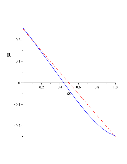
Figure 1: The thermodynamic curvature as a function of $\alpha$. The dash-dot line corresponds to the thermodynamic curvature for the classical limit for an isotherm and $z=0.01$. The solid line corresponds to the small deviation from the classical limit and represents the thermodynamic curvature at $z=0.3$.

It can be seen that the values of the thermodynamic curvature are different from the classical limit. It is interesting that the zero point of the thermodynamics curvature is shifted from $\alpha=\frac{1}{2}$ (classical limit) to the lower numbers. This means that quantum corrections change the value of $\alpha$ where we have a free non-interacting gas. This is the basic result of this paper.

The thermodynamic curvature for $\alpha=\frac{1}{2}$ can be worked out in the full physical range. For this special case, Eq. (8) becomes a quadratic equation which can be easily solved to give:

$$n_{i}=\frac{1}{\sqrt{\frac{1}{4}+\zeta^{2}}}.$$ (44)

Thus, the internal energy and particle number can be obtained,

$$U = \frac{8\pi Vmz\beta^{2}}{\hbar^{2}}\,{{}_{3}F_{2}}\left(\frac{1}{2},\frac{1}{2},\frac{1}{2};\frac{3}{2},\frac{3}{2};-\frac{z^{2}}{4}\right)$$

$$N = \frac{4\pi Vm\beta}{\hbar^{2}}{\it arcsinh}\left(\frac{z}{2}\right).$$ (45)

Calculation of the thermodynamic curvature is straightforward and the result is represented in Fig. (2). It shows that for $\alpha=\frac{1}{2}$, the thermodynamic curvature is zero only at the classical limit.

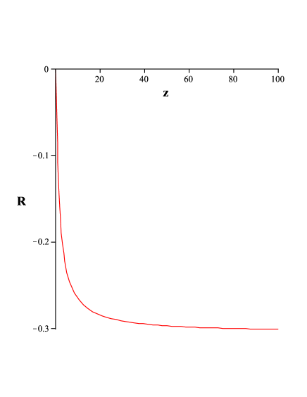
Figure 2: The thermodynamic curvature as a function of z (fugacity) for $\alpha=\frac{1}{2}$ and an isotherm in the full physical range.

5 Conclusion

The ideal anyonic gas in the Calssical limit has two different behaviour depending on whether $\alpha<\frac{1}{2}$ or $\alpha>\frac{1}{2}.$ For $\alpha<\frac{1}{2}$, the statistical interaction is attractive and the scalar thermodynamic curvature is positive. Thus, we may call the ideal anyonic gas in this case ”Bose-like”. Along these lines, the statistical interaction is repulsive for $\alpha<\frac{1}{2}$ and the scalar thermodynamic curvature is negative. Thus, the ideal anyonic gas in this case is ”Fermi-like”. As shown in [9, 27], we may consider the thermodynamic curvature as a measure of the stability of the system: the bigger the value of $R$, the less stable is the system. Therefore, the ideal anyonic gas in a Fermi-like case ($\alpha>\frac{1}{2}$) is more stable than in the Bose-like case ($\alpha<\frac{1}{2}$). Deviations from the classical limit move the zero point of the thermodynamic curvature from $\alpha=\frac{1}{2}$ to the lower values.

References

- [1] G. Ruppeiner, Phys. Rev. A 20, 1608 (1979).
- [2] G. Ruppeiner, Rev. Mod. Phys. 67, 605 (1995).
- [3] F. Weinhold, J. Chem. Phys. 63, 2479 (1975).
- [4] R. Mrugała, Physica A 125, 631 (1984).
- [5] P. Salamon, J. D. Nulton and E. Ihrig, J. Chem. Phys. 80, 436 (1984).
- [6] J. D. Nulton and P. Salamon, Phys. Rev. A 31, 2520 (1985).
- [7] G. Ruppeiner and C. Davis, Phys. Rev. A 41, 2200 (1990).
- [8] G. Ruppeiner, Phys. Rev A 44, 3583 (1991).
- [9] H. Janyszek and R. Mrugała, J. Phys. A: Math. Gen. 23, 467-476 (1990).
- [10] H. Janyszek and R. Mrugała, Phys. Rev. 39, 6515 (1989).
- [11] D. Brody and N. Rivier, Phys. Rev. E 51, 1006 (1995).
- [12] K. Kaviani and A. Dalafi-Rezaie, Phys. Rev. E 60, 3520 (1999).
- [13] D.A. Johnston, W. Janke and R. Kenna, Acta Phys. polon. B 34, 4923 (2003).
- [14] W. Janke, D.A. Johnston and R. Kenna, Phsica A 336, 181 (2004).
- [15] G. Ruppeiner, Phys. Rev. E 72, 016120 (2005).
- [16] G. Ruppeiner, Phys. Rev. D 75, 024037 (2007).
- [17] B. Mirza and M. Zamani-Nasab, JHEP 06, 059 (2007).
- [18] J. M. Leinaas and J. Myrheim, Nuovo Cimento 37B, 1 (1997).
- [19] F. Wilczek, Phys. Rev. Lett. 49, 957 (1982).
- [20] B. I. Halperin, Phys. Rev. Lett. 52, 1583 (1984).
- [21] F.D.M. Haldane, Phys. Rev. Lett. 67, 937 (1991).
- [22] Y.-S. Wu, Phys. Rev. Lett. 73, 922 (1994).
- [23] T. Aoyama, Eur. Phys. J. B 20, 123 (2001).
- [24] W.H. Huang, Phys. Rev B 53, 15842 (1996).
- [25] W.H. Huang, Phys. Rev E 51, 3729 (1995).
- [26] I. S. Gradshteyn and I. M. Ryxhik, Table of Inegrals, Series and Products (Fifth Edition), Academic Press, Inc. (1994).
- [27] H. Janyszek, J. Phys. A: Math. Gen. 23, 477-490 (1990).