Complexifications of Morse functions and the directed Donaldson-Fukaya category

Abstract.

Let $N$ be a closed four dimensional manifold which admits a self-indexing Morse function $f:N\longrightarrow\mathbb{R}$ with only 3 critical values $0$, $2$, $4$, and a unique maximum and minimum. Let $g$ be a Riemannian metric on $N$ such that $(f,g)$ is Morse-Smale. We construct from $(N,f,g)$ a certain six dimensional exact symplectic manifold $M$, together with some exact Lagrangian spheres $V_{4}$, $V_{2}^{j}$, $V_{0}$ in $M$, $j=1,\ldots,k$. These spheres correspond to the critical points $x_{4}$, $x_{2}^{j}$, $x_{0}$ of $f$, where the subscript indicates the Morse index. (In a companion paper we explain how $(M,V_{4},\{V_{2}^{j}\},V_{0})$ is a model for the regular fiber and vanishing spheres of the complexification of $f$, viewed as a Lefschetz fibration on the disk cotangent bundle $D(T^{*}N)$.) Our main result is a computation of the Lagrangian Floer homology groups

$$HF(V_{4},V_{2}^{j}),\,HF(V_{2}^{j},V_{0}),\,HF(V_{4},V_{0})$$

and the triangle product

$$\mu_{2}:HF(V_{4},V_{2}^{j})\otimes HF(V_{2}^{j},V_{0})\longrightarrow HF(V_{4},V_{0})$$

in terms of the Morse theory of $(N,f,g)$. The outcome is that the directed Donaldson-Fukaya category of $(M,V_{4},\{V_{2}^{j}\},V_{0})$ is isomorphic to the flow category of $(N,f,g)$.

1. Introduction

This paper is a natural sequel to [J09A], although it does not rely on the results there. In that paper we consider the following problem. Suppose that $N$ is a real analytic manifold and $f:N\longrightarrow\mathbb{R}$ is a real analytic Morse function. Then, in local charts on $N$, $f$ is represented by some convergent power series with real coefficients; if we complexify these local power series to get complex analytic power series (with the same coefficients) we obtain a complex analytic map on the disk bundle of $T^{*}N$ of some small radius,

$$f_{\mathbb{C}}:D(T^{*}N)\longrightarrow\mathbb{C},$$

called the complexification of $f$. In favorable circumstances, $f_{\mathbb{C}}$ can be regarded as a symplectic Lefschetz fibration. (Obviously this description is a little imprecise, but for us $f_{\mathbb{C}}$ will only be used for motivation; one possibility for a precise version is given in [HK08].)

Problem.

Describe the generic fiber of $f_{\mathbb{C}}$ as a symplectic manifold $M$, and describe its vanishing spheres as Lagrangian spheres in $M$.

Implicit in this problem is the more informal question: To what extent is the Morse theory of $f$ reflected in the complex geometry of $f_{\mathbb{C}}$? Problems of this type have been considered for some time in various fields, see for example [K78], [LS91], [AMP05], [AC99]. In fact we draw a great deal of inspiration from the last mentioned paper, which solves the above problem when $f:\mathbb{R}^{2}\longrightarrow\mathbb{R}$ is a real polynomial.

Our approach in [J09A] is as follows. We first take a Riemannian metric $g$ such that $(f,g)$ is Morse-Smale and we only assume $(N,f,g)$ is smooth, not necessarily real analytic. Then, given the corresponding handle decomposition of $N$, we construct an exact symplectic manifold $M$ of dimension $2\,\textup{dim}N-2$ together with some exact Lagrangian spheres $V_{1},\ldots,V_{m}\subset M,$ one for each critical point of $f$. (See §2 for the construction of $(M,V_{1},\ldots,V_{m})$ in the simple case $N=\mathbb{R}P^{2}$; see also §4a, 4b for a sketch of the four dimensional case.) Given $(M,V_{1},\ldots,V_{m})$, there is a unique (up to deformation) symplectic Lefschetz fibration $\pi:E\longrightarrow\mathbb{C}$, with regular fiber $M=\pi^{-1}(b)$ and vanishing spheres $V_{1},\ldots,V_{m}$ (see [S08, §16e]). Theorem $A$ below shows that $(E,\pi)$ and $(D(T^{*}N),f_{\mathbb{C}})$ have the same salient features. In this sense $(E,\pi)$ is a good model for $(D(T^{*}N),f_{\mathbb{C}})$ and $(M,V_{1},\ldots,V_{m})$ is very likely a correct answer to the above problem. In any case, for this paper and other applications (see [J09A] and below) we need not use $f_{\mathbb{C}}$; instead we will always use $(E,\pi)$.

Theorem A ([J09A]).

Assume $N$ is a smooth closed manifold and $f:N\longrightarrow\mathbb{R}$ is self-indexing Morse function with either two, three, or four critical values: $\{0,n\}$, $\{0,n,2n\}$, or $\{0,n,n+1,2n+1\}$. Let $(M,V_{1},\ldots,V_{m})$ be the data from the construction we discussed above (which depends in addition on a Riemannian metric $g$ on $N$ such that $(f,g)$ is Morse-Smale). Let $\pi:E\longrightarrow\mathbb{C}$ be the corresponding symplectic Lefschetz fibration with fiber $M$ and vanishing spheres $(V_{1},\ldots,V_{m})$. Then,

• $N$ embeds in $E$ as an exact Lagrangian submanifold;

• all the critical points of $\pi$ lie on $N$, and in fact $Crit(\pi)=Crit(f)$; and,

• $\pi|N=f:N\longrightarrow\mathbb{R}$ (up to reparameterizing $N$ and $\mathbb{R}$ by diffeomorphisms).

The hypotheses on $f$ ensure that the construction of $M$ is relatively easy. If there are five or more critical values then constructing $M$ becomes more complicated, so that is postponed for later treatment. In [J09A] we also sketch a proof that $E$ is homotopy equivalent to $N$, and we explain why $E$ is expected to be conformally exact symplectomorphic to $D(T^{*}N)$.

In this paper we consider the simplest nontrivial case, where $f$ is self-indexing and takes only three critical values $0$, $n$, $2n$, with a unique maximum and minimum. Furthermore, we focus on the case $\textup{dim}N=4$, firstly for the sake of concreteness and secondly because the stock of examples is most rich in that dimension (see [J09A] and the references there). (Everything in this paper can be done in an arbitrary dimension $\textup{dim}N=2n$ in a completely analogous way, see §4i for a sketch.) Thus, we assume $f$ has critical points $x_{4}$, $x_{2}^{j}$, $x_{0}$, $j=1,\ldots,k$, where the subscript indicates the Morse index, and we choose a Riemannian metric $g$ such that $(f,g)$ is Morse-Smale.

Using $(N,f,g)$ we will construct $M$ and $V_{4}$,$V_{2}^{j}$,$V_{0}$, $j=1,\ldots,k$ in a self-contained way (see §5 and §6). Then the purpose of this paper is to compute, for each $j$, the Lagrangian Floer homology groups

(1.1) $$HF(V_{4},V_{2}^{j}),\,HF(V_{2}^{j},V_{0}),\,HF(V_{4},V_{0})$$

and the triangle product (defined by counting holomorphic triangles in $M$ with boundary on $V_{4},V_{2}^{j},V_{0}$):

(1.2) $$\mu_{2}:HF(V_{4},V_{2}^{j})\otimes HF(V_{2}^{j},V_{0})\longrightarrow HF(V_{4},V_{0}).$$

To carry out these calculations we do not need to know that $M$ and $V_{4}$, $V_{2}^{j}$, $V_{0}$ can be viewed as the fiber and vanishing spheres of a Lefschetz fibration satisfying the conditions in Theorem $A$. Nevertheless, this viewpoint is very helpful for understanding why we would want to compute (1.1) and (1.2). Before discussing that, we first explain what the answer is; not surprisingly, it can be expressed nicely in terms of the Morse theory of $(N,f,g)$. Given $x,y\in Crit(f)$, let $Flow^{\,\circ}(x,y)$ be the space of unparameterized $(f,g)$-gradient trajectories from $x$ to $y$, and let $Flow(x,y)$ denote its compactification, which is obtained by allowing broken trajectories (possibly broken many times). This can be viewed a manifold with corners (see [HWZ06]) and for any $x,y,z\in Crit(f)$ with decreasing Morse indices, $Flow(x,y)\times Flow(y,z)$ embeds into $Flow(x,z)$ as a boundary face. The flow category of $(N,f,g)$, which first appeared in [CJS95], is defined as follows:

• The objects are the critical points of $f$.

• The morphism space from $x$ to $y$ is $H_{*}(Flow(x,y))$.

• Composition $\mu^{Flow}:H_{*}(Flow(x,y))\otimes H_{*}(Flow(y,z))\longrightarrow H_{*}(Flow(x,z))$ is induced by the inclusion $Flow(x,y)\times Flow(y,z)\subset Flow(x,z)$ combined with the Künneth isomorphism.

In our case it is not difficult to explicitly compute the flow category of $(N,f,g)$ (see §3). The main result of this paper of this paper is then as follows.

Theorem B.

Let $(N,f,g)$ and $(M,V_{4},\{V_{2}^{j}\},V_{0})$ be as above. Then

$$HF(V_{4},V_{2}^{j})\cong H_{*}(Flow(x_{4},x_{2}^{j})),\phantom{bbb}HF(V_{2}^{j},V_{0})\cong H_{*}(Flow(x_{2}^{j},x_{0})),$$

$$HF(V_{4},V_{0})\cong H_{*}(Flow(x_{4},x_{0})),$$

and, under this correspondence, the triangle product

$$\mu_{2}:HF(V_{4},V_{2}^{j})\otimes HF(V_{2}^{j},V_{0})\longrightarrow HF(V_{4},V_{0})$$

coincides with the composition in the Flow category

$$\mu^{Flow}:H_{*}(Flow(x_{4},x_{2}^{j}))\otimes H_{*}(Flow(x_{2}^{j},x_{0}))\longrightarrow H_{*}(Flow(x_{4},x_{0})).$$

See §2 for an explanation of this theorem in the case $N=\mathbb{R}P^{2}$; see also §4h for a sketch of the four dimensional case.

Let us now return to the question of why we would want to compute (1.1) and (1.2), and why Theorem $B$ is a useful answer. To this end, we make a brief digression and explain some of the results in Seidel’s recent book [S08]. One of the main results [S08, Corollary 18.25 plus Proposition 18.14] says that, for any Lefschetz fibration $\pi:E\longrightarrow\mathbb{C}$, the Lefschetz thimbles $\Delta_{1},\ldots,\Delta_{m}\subset E$ in a certain sense generate the whole Fukaya category $Fuk(E)$. In other words, each exact Lagrangian submanifold $L\subset E$ can be expressed as a certain algebraic combination of $\Delta_{1},\ldots,\Delta_{m}\subset E$ (intuitively, $L$ is geometrically obtained from $\Delta_{1},\ldots,\Delta_{m}\subset E$ by surgery theoretic operations; see [J09A]). We will refer to this informally as the Seidel decomposition of $L$. This generating property highlights the importance of the sub-category with objects $\Delta_{1},\ldots,\Delta_{m}$ and morphisms $CF(\Delta_{i},\Delta_{j})$. Now, the Lefschetz thimbles only intersect one another in a fixed regular fiber $M$ at points in the corresponding vanishing spheres $V_{1},\ldots,V_{m}\subset M$. Therefore, we expect $CF(\Delta_{i},\Delta_{j})$ (which is computed in $E$) to be equal to $CF(V_{i},V_{j})$ (which is computed in $M$). However, because $\Delta_{1},\ldots,\Delta_{m}$ are not closed one needs to choose some perturbation convention in the definition of $CF(\Delta_{i},\Delta_{j})$. The standard choice involves a natural ordering on $\Delta_{1},\ldots,\Delta_{m}$ given by the counter clock-wise ordering of the vanishing paths (see [S08B, §2] for further informal discussion about this). The upshot is that, in fact, $\Delta_{1},\ldots,\Delta_{m}$ form a directed sub-category, with morphisms

(1.3) $$CF(\Delta_{i},\Delta_{j})\cong\left\{\begin{matrix}CF(V_{i},V_{j})&\hbox{ if }i>j\\ \mathbb{K}&\hbox{ if }i=j\\ 0&\hbox{ if }i<j\end{matrix}\right.$$

where $\mathbb{K}$ is the base ring and we think of $CF(\Delta_{i},\Delta_{i})\cong\mathbb{K}$ as generated by an identity element $e$. So, we can forget about the Lefschetz thimbles if we wish, and define the directed Fukaya category of $(M,V_{1},\ldots,V_{m})$ to be the $A_{\infty}$ category with objects $V_{1},\ldots,V_{m}$ and morphisms $Hom(V_{i},V_{j})$ given by the right-hand side of (1.3); this is denoted $Fuk^{\rightarrow}(M,V_{1},\ldots,V_{m})$, and it is also known as the Seidel-Fukaya category (see [S00A, S08B, S08] for more about this).

Thus, what we are computing in Theorem $B$ is the directed Fukaya category of $(M,V_{4},\{V_{2}^{j}\},V_{0})$, but at the level of homology; we call this the directed Donaldson-Fukaya category, and denote it $H(Fuk^{\rightarrow}(M,V_{4},\{V_{2}^{j}\},V_{0}))$. (Here there are only three levels in the ordering, corresponding to the three critical values $0,2,4$; thus all $V_{2}^{1},\ldots,V_{2}^{k}$ are on equal footing.) So we can re-formulate Theorem $B$ as follows:

Theorem $B\,^{\prime}$.

The directed Donaldson-Fukaya category of $(M,V_{4},\{V_{2}^{j}\},V_{0})$ is isomorphic to the flow category of $(N,f,g)$.

This result was essentially conjectured by Seidel in [S00B, §8]. For an arbitrary Lefschetz fibration it is not realistic to hope for an explicit computation of (1.1) and (1.2) because the regular fiber and vanishing spheres are often hard to describe. But in our case we have a simple explicit model $(M,V_{4},V_{2}^{j},V_{0})$ for these, and the vanishing spheres $V_{4},V_{2}^{j},V_{0}\subset M$ are also highly symmetric; this is what makes Theorem $B$ or $B^{\prime}$ feasible.

Remark 1.1.

In our situation, the directed Donaldson-Fukaya category, given by (1.1) and (1.2), is actually very close to the chain level version. This is because there are only two products: $\mu_{1}$ (the Floer differential), and $\mu_{2}$; all higher order products $\mu_{3},\mu_{4},\ldots$ are zero, because there are only three levels in the directed category.

Thus, Theorem $B$ or $B^{\prime}$ has a certain amount of intrinsic interest, as it provides a simple description of an important invariant attached to some natural Lefschetz fibrations on cotagent bundles (assuming $E\cong D(T^{*}N)$ in Theorem $A$ for simplicity). The answer moreover reflects the expected close relationship between the complex geometry of $(E,\pi)$ and the Morse theory of $(N,f,g)$ (recall $\pi$ is a model for the complexification of $f$). In the larger scheme it fits in with many other results relating Floer theoretic invariants of cotangent bundles $T^{*}N$ to more classical invariants of the base $N$, as in [F89, FO97, AS06, V98, N07, NZ07].

On a more practical level there are a couple of reasons why this explicit answer in terms of the flow category is of interest as well. The most immediate application we have in mind is to use Seidel’s decomposition (which we discussed above) in combination with Theorems $A$ and $B$ to study Lagrangian submanifolds in $T^{*}N$. One basic goal is to prove that any closed exact Lagrangian $L\subset T^{*}N$ is Floer theoretically equivalent to $N$. This means in particular that $HF(L,L)\cong HF(N,N)$, so that $H^{*}(L)\cong H^{*}(N)$, and $HF(L,T_{x}^{*}N)\cong HF(N,T_{x}^{*}N)$, so that $deg(L\longrightarrow N)=\pm 1$. Of course, results of this kind have been obtained for arbitrary spin manifolds $N$ in [FSS08, FSS07] and [N07] (for simply-connected $N$). We want to consider a slightly different approach along the lines of the quiver-theoretic approach for the case $N=S^{n}$ in [S04]. Because this approach is more explicit it is expected to yield somewhat more refined results. For example, we should be able to remove one significant assumption on $L$, namely that it has vanishing Maslov class $\mu_{L}\in H^{1}(L)$.

Here is a concrete example which illustrates how Theorem $B$ makes Seidel’s decomposition very explicit. Take $N=\mathbb{C}P^{2}$ with its standard handle-decomposition, corresponding to a Morse-Smale pair $(f,g)$, where $f$ has three critical points $x_{0},x_{2},x_{4}$, with Morse indices $0,2,4$. Then the flow category of $(N,f,g)$ is relatively easy to compute (see §3); it is given by the following quiver with relations:

(1.6)

$$b_{1}a_{1}=0,\,b_{0}a_{0}=c_{0},\,b_{0}a_{1}-b_{1}a_{0}=c_{1}$$

By Theorem $A$, there is a Lefschetz fibration $(E,\pi)$ corresponding to $(N,f,g)$, which models the complexification of $f$ on $D(T^{*}N)$. By construction, $\pi$ comes with an explicit regular fiber $M$ and vanishing spheres $V_{0},V_{2},V_{4}\subset M$. Theorem $B$ or $B^{\prime}$ says that the directed Donaldson Fukaya category of $(M,V_{4},V_{2},V_{0})$ is represented by the exact same quiver (1.6), except we replace the labels $x_{4},x_{2},x_{0}$ on the vertices by $V_{4},V_{2},V_{0}$:

(1.9)

$$b_{1}a_{1}=0,\,b_{0}a_{0}=c_{0},\,b_{0}a_{1}-b_{1}a_{0}=c_{1}$$

Now, let $L\subset T^{*}N$ be any closed exact Lagrangian submanifold. Theorem $A$ also says we have an exact Lagrangian embedding $N\subset E$. Consequently there is an exact Weinstein embedding $D(T^{*}N)\subset E$. By rescaling $L\leadsto\epsilon L$ by some small $\epsilon>0$, we get an exact Lagrangian embedding $L\subset E$. Now the Seidel decomposition applied to $L\subset E$ says that $L$ can be expressed in terms of the Lefschetz thimbles of $\pi$, say $\Delta_{4},\Delta_{2},\Delta_{0}\subset E$. But as we discussed earlier, this is equivalent to saying that $L$ can be expressed in terms of the directed Fukaya category of the corresponding vanishing spheres $V_{4},V_{2},V_{0}$, given by the quiver (1.9). In our example this has the following concrete meaning: $L$ is represented by a certain quiver representation of (1.9):

(1.12)

$$B_{1}A_{1}=0,\,B_{0}A_{0}=C_{0},\,B_{0}A_{1}-B_{1}A_{0}=C_{1}$$

Here, a quiver representation, such as (1.12), is just a choice of vector-spaces $W_{4}$, $W_{2}$, $W_{0}$ at each vertex, and a choice of linear maps $A_{0},A_{1},B_{0},B_{1},C_{0},C_{1}$ satisfying the given relations (the particular quiver representation (1.12) corresponding to $L$ is determined by $W_{i}=HF(L,\Delta_{i})$ and the triangle products $W_{i}\otimes HF(\Delta_{i},\Delta_{j})\longrightarrow W_{j}$). To show $L$ is Floer theoretically equivalent to $N$ in $T^{*}N$ is equivalent to showing that the representation (1.12) is necessarily isomorphic to the representation

$$W_{4}=W_{2}=W_{0}=\mathbb{C},\,A_{0}=B_{0}=C_{0}=id,\,A_{1}=B_{1}=C_{1}=0.$$

(Of course, this is the representation corresponding to $N\subset T^{*}N$.) The analogous problem for $N=S^{n}$ was solved in [S04].

To round off the discussion we mention one other potential application which stems from the close relationship between the Flow category of $N$ and the category of constructible sheaves on $N$. Our aim is to describe the relationship between two recent successful approaches for analyzing the Fukaya category of cotagent bundles (see [FSS07] for a detailed comparison). One approach, due to Fukaya, Seidel, and Smith [FSS08], is based on Lefschetz fibrations and Picard-Lefschetz theory, as in [S08]. The other approach, due to Nadler and Zaslow [NZ07, N07], relates Lagrangian submanifolds in $T^{*}N$ to constructible sheaves on $N$, and is based on the characteristic cycle construction of Kashiwara-Shapira [KS94]. (There is also a third approach in progress, based on a Leray-Serre type spectral sequence, see [FSS07], and above we discussed a fourth quiver-theoretic approach which expands on [S04].) Now, if $N$ is real analytic, the flow category of $N$ (more precisely, the derived category of the chain level version) is expected to be equivalent to the derived category of constructible sheaves on $N$ (constructible with respect to the stratification by unstable manifolds of $f$), see [S00B, Remark 7.1]. This conjecture of Seidel combined with Theorem $B^{\prime}$ (extended slightly to the chain level as in remark 1.1) leads to a direct way of comparing the two viewpoints [FSS08] and [NZ07, N07] described above. More precisely, we have the following (commutative) diagram, where each arrow is either an isomorphism or an equivalence (below the $D$’s are for derived categories).

Here, $Fuk_{NZ}(T^{*}N)$ and $Fuk_{S}(T^{*}N)$ denote two versions of the Fukaya category of $T^{*}N$, due to Nadler-Zaslow and Seidel respectively. The difference lies in the choice of noncompact Lagrangians they allow (see [FSS07]). It is believed that their derived categories are equivalent, but to the author’s knowledge no proof has been nailed down yet (this equivalence is of interest in particular for applications to the homological mirror symmetry conjecture [FLTZ09, FLTZ09]). One consequence of the above diagram is this desired equivalence (the top dotted arrow), though it may be easier and more enlightening to find a direct correspondence. Assuming the existence of such a natural correspondence, and replacing the dotted arrow by that, it is also interesting to ask if the above diagram commutes; the diagram represents a parallelism between Picard-Lefschetz theory and the characteristic cycle functor.

Overview and organization

In this paper our focus is on giving a precise proof of Theorem B (see Proposition 7.4 and Theorem 10.1). The crucial point is that $V_{4}$,$V_{2}^{j}$,$V_{0}$ have a certain rotational symmetry, and this allows us to compute the moduli space of holomorphic triangles explicitly. On the other hand, this means we cannot perturb $V_{4}$,$V_{2}^{j}$,$V_{0}$ to make them transverse, as one usually does to compute Floer homology, and therefore the whole calculation must be done in the context of Morse-Bott Floer homology. In that theory the Lagrangian submanifolds are allowed to intersect in a Morse-Bott fashion along submanifolds, and the Floer complex is generated by cycles in the intersection components. We use Morse cycles as in [PSS94], [S98], [F04], since that is the cleanest known approach. In the interest of brevity we do not treat signs and gradings for Morse-Bott Floer homology in this paper. Consequently, Theorem B is limited for the moment to $\mathbb{Z}/2$ coefficients and ungraded Floer groups.

The paper is basically split into three parts. The first part (§2–4) outlines the main lines of argument in two warm-up sections: §2 treats the simple case $N=\mathbb{R}P^{2}$, and §4 outlines the paper in detail in the case $N=\mathbb{C}P^{2}$. In §3 we compute the flow category of $(N,f,g)$ under the assumptions of Theorem $B$. From these (especially §4) the reader can get a very good idea of the proof of Theorem $B$, including all the pitfalls one has to watch for. The rest of the paper gives the complete details. The second part (§5–10) contains the main line of argument. Along the way we refer to the third part (§11–13), which is where the main technical work is done: In §11 we prove that the relevant moduli spaces of holomorphic strips are in 1-1 correspondence with the gradient flow lines of certain functions; in §12 we explicitly describe the moduli space of holomorphic triangles (inside a Weinstein neighborhood $D(T^{*}V_{2}^{j})\subset M$ of each $V_{2}^{j}$). In §13 we provide an appendix which explains the definition and main features of Morse-Bott Floer homology in some special cases sufficient for our purposes. The paper is basically written in the intended order of reading, with the exception of the last section, which should be referred to as necessary. Some Floer theory notation and conventions are in sections 13a, 13b. We use the notation $\nu^{*}K\subset T^{*}N$ for the conormal bundle of $K\subset N$.

Acknowledgements

The results of this paper are based on my Ph.D. thesis, carried out at the University of Chicago from 2003-2006 under the supervision of Paul Seidel. Of course, this paper owes much to him. Thanks also go to Frédéric Bourgeois, Kenji Fukaya, Kaoru Ono, and Helmut Hofer for help with Fredholm theory in Morse-Bott Floer homology, to Felix Schmäschke for pointing out several notational mistakes in an earlier draft, and to Urs Frauenfelder for patiently answering many questions about Morse-Bott homology. An extra big thanks goes to Peter Albers for frequent sanity checks and many helpful discussions about Floer theory.

2. A simple example: $N=\mathbb{R}P^{2}$

To illustrate the main ideas of this paper, we first consider the two dimensional example $N=\mathbb{R}P^{2}$, where we take the self-indexing standard Morse function $f:\mathbb{R}P^{2}\longrightarrow\mathbb{R}$ which has 3 critical points $x_{2},x_{1},x_{0}$, with the standard flow lines as in figure 2. In this section we will explain several things in this simple example. First, we explain a natural construction of the complexification of $f$ on the disk cotangent-bundle of $D(T^{*}\mathbb{R}P^{2})$ from elementary algebraic geometry; it is quite different from the construction we give for $(E,\pi)$ in [J09A, Theorem A], but it gives a useful additional viewpoint. (In most examples this approach would not work.) After that we explain the construction of $(M,V_{2},V_{1},V_{0})$ (see figure 3) using the topological method we will use in this paper (and in [J09A]). We also briefly explain how the construction relates to Morse theory, and we explain roughly why the vanishing spheres are defined as they are. We note that $(M,V_{2},V_{1},V_{0})$ is isomorphic to the regular fiber and vanishing spheres of algebreo-geometrically constructed Lefschetz fibration from before. Finally, we sketch the proof of Theorem $B$ in this simple low-dimensional case by inspecting $(M,V_{2},V_{1},V_{0})$ and the flow lines of $f$ on $\mathbb{R}P^{2}$.

2a. An algebreo-geometric construction of the complexification

The complexification $f_{\mathbb{C}}:D(T^{*}\mathbb{R}P^{2})\longrightarrow\mathbb{C}$ can be viewed as the restriction of a well-known Lefschetz pencil in algebraic geometry. Namely, in [A03, p. 19] (or [S00B, p.7,27], or [AS04, p. 39]) one finds the example of a Lefschetz pencil on $\mathbb{C}P^{2}$ formed by two homogeneous degree 2 polynomials $\sigma_{0},\sigma_{1}$ with real coefficients. The base locus $B=\{\sigma_{0}=\sigma_{1}=0\}$ consists of four points. If we delete a neighborhood $U$ of the fiber at infinity $\{\sigma_{0}=0\}$ (we assume $\sigma_{0}$ has no zeros on $\mathbb{R}P^{2}$) we will in particular delete this base locus from every fiber. Thus we obtain a Lefschetz fibration

$$\pi=\sigma_{1}/\sigma_{0}:\mathbb{C}P^{2}\setminus U\longrightarrow\mathbb{C}.$$

Because $\sigma_{0},\sigma_{1}$ have degree 2, the regular fiber of the pencil is a 2-sphere. When we delete a neighborhood of the base locus the regular fiber becomes $S^{2}$ with four small disks removed; this is the regular fiber of $\pi=\sigma_{1}/\sigma_{0}$ on $\mathbb{C}P^{2}\setminus U$. There are three singular fibers each of which consists of a pair of 2-spheres which touch at a single point; each of the two 2-spheres contains two of the four base points. The three singular fibers correspond to the three ways of splitting up the four base into pairs. Thus, there are three vanishing spheres in the regular fiber, which divide the four holes in the fiber into pairs in all three possible ways, see figure 1 (see also [A03, p. 19] or [AS04, p. 39]).

Figure 1. The regular fiber of the pencil $\pi=\sigma_{1}/\sigma_{0}$ (with the four base points deleted) and the three vanishing spheres.

To see that $\pi$ is a complexification, consider

$$f=\pi|\mathbb{R}P^{2}:\mathbb{R}P^{2}\longrightarrow\mathbb{R}.$$

If $\sigma_{0}$, $\sigma_{1}$ are chosen suitably then the critical points of $\pi$ lie on $\mathbb{R}P^{2}$ and $f$ isotopic to the standard Morse function with three critical points. Furthermore one can show using the Liouville flow that there is a Weinstein tubular neighborhood of $\mathbb{R}P^{2}\subset\mathbb{C}P^{2}$ which fills out all of $\mathbb{C}P^{2}\setminus U$; thus $\mathbb{C}P^{2}\setminus U\cong D(T^{*}\mathbb{R}P^{2})$ and $\pi$ is the complexification of $f$.

2b. Topological construction of $M$

Take a Riemannian metric $g$ on $\mathbb{R}P^{2}$ such that $(f,g)$ is a Morse-Smale pair, where $f$ has 3 critical points $x_{2},x_{1},x_{0}$, with the standard flow lines as in figure 2.

Figure 2. The flow lines of $(f,g)$ on $\mathbb{R}P^{2}$.

To define $M$, let $V_{0}=V_{1}=S^{1}$. Then take the unit disk bundles with respect to the standard metrics on the cotangent bundles, $D(T^{*}V_{0})$ and $D(T^{*}V_{1})$. The short answer to constructing $M$ is to take two copies of $S^{0}$, say $K_{0}\subset V_{0}$ and $K_{1}\subset V_{1}$ and plumb $D(T^{*}V_{0})$ and $D(T^{*}V_{1})$ together so that $V_{0}$ and $V_{1}$ meet along $S^{0}\cong K_{0}\cong K_{1}$. As usual, plumbing means we identify neighborhoods of $K_{0}$ and $K_{1}$ in $D(T^{*}V_{0})$ and $D(T^{*}V_{1})$ by identifying the fiber direction in one with the base direction in the other. More precisely, we take tubular neighborhoods of $K_{0},K_{1}$, say $S^{0}\times D^{1}\subset V_{0}$, $S^{0}\times D^{1}\subset V_{1}$ and we trivialize the disk bundles $D(T^{*}V_{0})$ and $D(T^{*}V_{1})$ over these neighborhoods

$$D(T^{*}V_{0})|_{(S^{0}\times D^{1})},\,D(T^{*}V_{1})|_{(S^{0}\times D^{1})}\cong S^{0}\times D^{1}\times D^{1}.$$

Then we glue $D(T^{*}V_{0})$ to $D(T^{*}V_{1})$ along $D(T^{*}V_{0})|_{S^{0}\times D^{1}}$ and $D(T^{*}V_{1})|_{S^{0}\times D^{1}}$ using the map $(x,y)\mapsto(-y,x):D^{1}\times D^{1}\longrightarrow D^{1}\times D^{1}.$ (We have a minus sign to ensure this map is symplectic.)

Depending on the orientations of the identifications

(2.13) $$D(T^{*}V_{0})|_{S^{0}\times D^{1}},\,D(T^{*}V_{1})|_{S^{0}\times D^{1}}\cong S^{1}\times D^{1}\times D^{1},$$

there may be twists (like a Möbius strip) in $D(T^{*}V_{0})$ or $D(T^{*}V_{1})$ after we plumb them together. For $N=\mathbb{R}P^{2}$ it turns out that there should be no twists in $D(T^{*}V_{0})$ or $D(T^{*}V_{1})$. (See below for how (2.13) is determined by Morse theory.) Thus $M$ is homeomorphic to $S^{2}$ with four small open disks removed (see figure 3). We say homeomorphic, rather than symplectomorphic, because $M$ has some corners. To remedy that, one can alternatively construct $M$ so that it has smooth contact type boundary by attaching two 1-handles to the boundary $D(T^{*}V_{0})$ using Weinstein’s technique [W91]. In this case the 1-handles should be attached to $\partial D(T^{*}V_{0})$ along the boundary of the disk conormal bundle $\partial D(\nu^{*}K_{0})\subset\partial D(T^{*}V_{0})$.

Let us now explain the connection to Morse theory. Above, $V_{0}$ and $V_{1}$ represent the vanishing spheres of $f_{\mathbb{C}}$ corresponding to $x_{0}$ and $x_{1}$. Let us assume that $f$ is self-indexing so that it has two regular level sets $f^{-1}(1/2)$ and $f^{-1}(3/2)$. The first step in relating the Picard-Lefschetz data to the Morse theory data is to identify

$$V_{0}=f^{-1}(1/2)\cong S^{1}.$$

Now $(f,g)$ determines the standard handle-decomposition of $\mathbb{R}P^{2}$ with three handles of index $0,1,2$. The 1-handle has an attaching sphere

$$K_{0}=S^{0}\subset S^{1}\cong f^{-1}(1/2)=V_{0}.$$

Moreover, we have a tubular neighborhood of $K_{0}\subset V_{0}$

$$\phi:S^{0}\times[-1,1]\longrightarrow S^{1}$$

determined up to isotopy by the framing we use to attach the 1-handle. Then $\phi$ in turn determines an exact symplectic identification

(2.14) $$\widehat{\phi}:D(T^{*}V_{0})_{(S^{0}\times[-1,1])}\longrightarrow S^{0}\times D^{1}\times D^{1},$$

where $D^{1}\times D^{1}\subset(\mathbb{R}^{2},dy\wedge dx)$, and the coordinates are $(x,y)\in\mathbb{R}^{2}$. On the other hand $V_{1}=S^{1}\subset\mathbb{R}^{2}$ has two standard $S^{0}$’s

$$K_{+}^{1}=\{(\pm 1,0)\}\text{ and }K_{-}^{1}=\{(0,\pm 1)\}.$$

($K_{-}^{1}$ will be used in the construction of $M$; $K_{+}^{1}$ will be used in the construction of $V_{2}$.) We take the canonical orientation preserving tubular neighborhood of $K_{-}^{1}$, $S^{0}\times[-1,1]\subset S^{1}$ and the corresponding exact symplectic trivialization

$$D(T^{*}V_{1})|_{(S^{0}\times[-1,1])}\cong S^{0}\times D^{1}\times D^{1}$$

which we use to plumb $D(T^{*}V_{0})$ and $D(T^{*}V_{1})$ together. The main point we wanted to make was, first, that the $S^{0}$ corresponds precisely to the intersection of the unstable manifold $U(x_{1})$ with the level set $V_{0}=f^{-1}(1/2)$, and second that the framing of the corresponding 1-handle determines the trivialization (2.14). (On the other hand, the corresponding trivialization for $D(T^{*}V_{1})$ is always the same; this is analogous to the set up in a handle attachment.)

2c. Construction of the vanishing spheres

We have already defined $V_{0},V_{1}$. We now explain how to define $V_{2}$ (see figure 3). The method we present here is the same as the one that we use in general. Let $\Phi$ denote the time $\pi/2$ geodesic flow on $D(T^{*}V_{1})$ (which is Hamiltonian). Consider the disk conormal bundle $D(\nu^{*}K_{+}^{1})\subset D(T^{*}V_{1})$ and set $H=\Phi(D(\nu^{*}K_{+}^{1}))$. Since $\Phi$ fixes points in the zero section, and moves covectors $v$ of length 1 a distance $\pi/2$ in the direction of $v$, we have $\partial H=\partial D(\nu^{*}K_{-}^{1})$ and $H\cap V_{1}=K_{+}^{1}$. Now tweak $\Phi$ slightly to get a new Hamiltonian diffeomorphism $\widetilde{\Phi}$ such that $\widetilde{H}=\widetilde{\Phi}(D(\nu^{*}K_{+}^{1}))$ agrees with $D(\nu^{*}K_{-}^{1})$ in a neighborhood of $\partial D(\nu^{*}K_{-}^{1})$. Then we define

$$V_{4}=(V_{0}\setminus D(\nu^{*}K_{-}^{1}))\cup\widetilde{H}.$$

See figure 3.

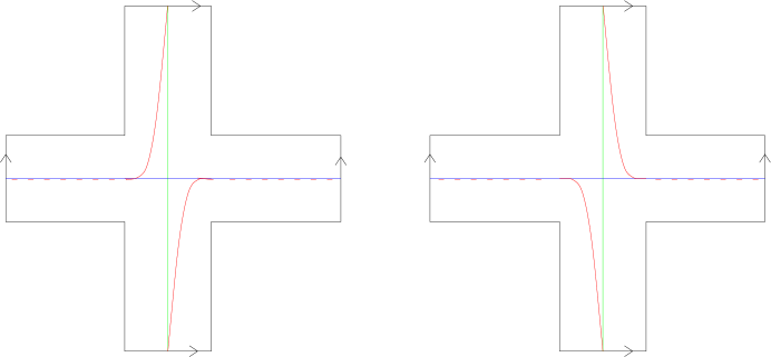
Figure 3. The fiber $M$ and vanishing spheres $V_{2}$ (red) $V_{1}$ (green), $V_{0}$ (blue) for $(\mathbb{R}P^{2},f,g)$. The edges labeled by letters ($a,b,c,d$) are identified according to the indicated orientations. The other labels correspond to generators in Floer homology $A_{1},A_{2}\in HF(V_{2},V_{1})$, $B_{1},B_{2}\in HF(V_{1},V_{0})$, $C_{1},C_{2}\in HF(V_{2},V_{0})$.

Notice that $V_{4}$ is obtained by surgery on $V_{0}$ along the framed attaching sphere $K_{0}\subset V_{0}$, just as $f^{-1}(3/2)$ is obtained by surgery on $f^{-1}(1/2)$. This is not a coincidence, as we now explain.

In this simple example it is worth giving a brief sketch of where the construction of fiber and vanishing spheres come from (see [J09A] for details). One should consider $M$ as being a model for the regular fiber of $f_{\mathbb{C}}:D(T^{*}N)\longrightarrow\mathbb{C}$ at the base point $b=1/2$. And one should think of $(V_{0},V_{1},V_{2})$ as being a model for the vanishing spheres in $M$ relative to the vanishing paths $\gamma_{0},\gamma_{1},\gamma_{2}$, as in figure 4. Namely, $\gamma_{0}$ parameterizes $[0,1/2]$, $\gamma_{1}$ parameterizes $[1/2,1]$, and $\gamma_{2}$ goes around the critical value $1$, by a half loop in the lower half plane, and then continues along the interval $[3/2,2]$.

Figure 4. The three vanishing paths $\gamma_{0},\gamma_{1},\gamma_{2}$.

The fact that $\gamma_{0}$ and $\gamma_{1}$ are straight line segments is reflected in the simplicity of $V_{0}$ and $V_{1}$. Also the identification of $V_{0}$ with $f^{-1}(1/2)$ makes sense in view of the fact the stable manifold of $x_{0}$ over $[0,1/2]$ is all of $f^{-1}([0,1/2])$ and so $f^{-1}([0,1/2])$ coincides with the Lefschetz thimble over $[0,1/2]$. On the other hand the half loop in $\gamma_{2}$ accounts for the twist in $V_{2}$. Indeed, if instead of $b=1/2$ we had the base point at $b^{\prime}=3/2$, with $\gamma_{2}^{\prime}$ parameterizing $[3/2,2]$, then the corresponding vanishing sphere $V_{2}^{\prime}$ would be identified with $f^{-1}(3/2)\subset f_{\mathbb{C}}^{-1}(3/2)$ and the Lefschetz thimble would be the unstable manifold $f^{-1}([3/2,1])$. Thus, $V_{2}^{\prime}\subset f_{\mathbb{C}}^{-1}(3/2)$ would look similar to $V_{0}$. But because $V_{2}\subset f_{\mathbb{C}}^{-1}(1/2)$ is actually obtained from $V_{2}^{\prime}\subset f_{\mathbb{C}}^{-1}(3/2)$ by parallel transport along the half loop, $V_{2}$ is twisted by something like a “half Dehn twist”.

We conclude this section by pointing out that since $V_{2}$,$V_{1}$,$V_{0}$ divide the four holes of $M$ into pairs in all three possible ways, the fiber and vanishing spheres we have constructed are equivalent to those of the algebreo-geometric example above.

2d. Comparing the Flow category and the directed Fukaya category

In the case $N=\mathbb{R}P^{2}$ Theorem $B$ was explained already in [S00B, p. 9,27]. The flow category of $(\mathbb{R}P^{2},f,g)$ has three objects $x_{2},x_{1},x_{0}$ and the space of morphisms from $x_{i}$ to $x_{j}$, for every $i>j$, is generated by two elements (both in degree 0). For example, from figure 2 one sees that $Flow(x_{2},x_{0})$ is diffeomorphic to the disjoint union of two closed intervals $I_{1},I_{2}$, where the gradient flow lines corresponding to $I_{1}$ (resp. $I_{2}$) fill out the top half (resp. bottom half) of the disk in figure 2. Let $A_{1},A_{2}$, $B_{1},B_{2}$, $C_{1},C_{2}$ denote the generators as labeled in figure 2. Thus the boundary of $I_{1}$ corresponds to the broken trajectories $B_{2}\circ A_{2}$ and $B_{1}\circ A_{1}$, and similarly $\partial I_{2}\cong\{B_{1}\circ A_{2},\,B_{2}\circ A_{1}\}$. Thus $B_{1}\circ A_{2}$ is homologous to $B_{2}\circ A_{1}$ in $Flow(x_{2},x_{0})$, and similarly $B_{2}\circ A_{2}\backsim B_{1}\circ A_{1}$. Therefore the flow category can be described as the following quiver with relations:

$$B_{2}A_{2}=B_{1}A_{1}=C_{1},\,\,B_{1}A_{2}=B_{2}A_{1}=C_{2}.$$

On the other hand, the directed Donaldson-Fukaya category of $(M,V_{2},V_{1},V_{0})$ has objects $V_{2},V_{1},V_{0}$ and the Floer homology groups are also each generated by two elements (of degree 0). (Indeed, the intersection of any two $V_{i}$’s is either a pair of points or a pair of intervals; to be more formal one should isotope $V_{2}$ so that the two intervals become two points.) By counting triangles in $M$ with boundary on $V_{2},V_{1},V_{0}$ one finds precisely the same quiver with relations as above. For example, in figure 3 one has four such triangles; the right-most one has vertices corresponding to $A_{1},B_{2},C_{2}$, and it gives rise to the relation $B_{2}A_{1}=C_{2}$ (see also [AS04, p. 39]).

3. Computing the flow category

Fix a closed 4-manifold $N$ which admits a self-indexing Morse function $f:N\longrightarrow[0,4],$ with critical values $0,2,4$ and with a unique maximum and minimum. Let $g$ be Riemannian metric such that $(f,g)$ is Morse-Smale. In this section we compute the flow category of $(N,f,g)$ in this case (see the introduction for the definition).

Let $L_{-}=f^{-1}(1)\cong S^{3}\text{ and }L_{+}=f^{-1}(3)\cong S^{3}.$ For each $j=1,\ldots,k$ we have two knots

$$K_{-}^{j}=U(x_{2}^{j})\cap L_{-}\cong S^{1}\text{ and }K_{+}^{j}=S(x_{2}^{j})\cap L_{+}\cong S^{1}.$$

Here $U(x)$ is the unstable manifold and $S(x)$ is the stable manifold. The handle decomposition of $N$ coming from $(f,g)$ has $k$ 2-handles with attaching spheres $K^{1}_{-}$, $\ldots,$ $K^{k}_{-}$. Let $\phi_{j}:S^{1}\times D^{2}\longrightarrow U_{j}$ denote the attaching map for the $j$th 2-handle where $U_{j}\subset L_{-}$ is a tubular neighborhood of $K_{-}^{j}$ in $L_{-}$. Set $U=\cup_{j=1}^{j=k}U_{j}$, $K_{\pm}=\cup_{j}K_{\pm}^{j}.$ The first step in the computation is to note the following result.

Lemma 3.1.

There are diffeomorphisms $Flow(x_{4},x_{2}^{j})\cong K_{+}^{j}$, $Flow(x_{2}^{j},x_{0})\cong K_{-}^{j}$, and $Flow(x_{4},x_{0})\cong L_{-}\setminus\textup{Int\,}(U)$.

Proof.

For the first two diffeomorphisms we use the map which associates to a trajectory $\gamma$ the corresponding intersection point in $\gamma\cap L_{-}\in L_{-}$ or $\gamma\cap L_{+}\in L_{+}$. For the second diffeomorphism, note first that

$$Flow^{\circ}(x_{4},x_{0})\cong L_{+}\setminus K_{+}\cong L_{-}\setminus K_{-}$$

by the same map. Now take the compactification $Flow(x,y)$ and delete an open collar neighborhood of the boundary to obtain an diffeomorphic manifold

$$\widetilde{Flow}(x,y)\cong Flow(x,y),\text{ with }\widetilde{Flow}(x,y)\subset Flow^{\circ}(x,y).$$

Now consider $L_{-}\setminus\textup{Int\,}(U)\subset L_{-}\setminus K_{-}$. Under the correspondence

$$Flow^{\circ}(x,y)\cong L_{-}\setminus K_{-},$$

$L_{-}\setminus\textup{Int\,}(U)$ also corresponds to $F(x,y)$ minus some collar neighborhood of the boundary, just like $\widetilde{Flow}(x,y)$. But any two complements of a collar neighborhood are diffeomorphic, so $Flow(x,y)\cong\widetilde{Flow}(x,y)\cong L_{-}\setminus\textup{Int\,}(U).$ ∎

For $H_{*}(K_{\pm}^{j})$ take the generators $[K_{\pm}^{j}]$, $[p_{\pm}^{j}]$, where $p_{\pm}^{j}\in K_{\pm}^{j}$. For $H_{*}(\partial U_{j})$ take the generators $[\partial U_{j}],\,\lambda_{j},\,\mu_{j},\,[q_{j}],$ where $q_{j}\in\partial U_{j}$ and $\lambda_{j},\,\mu_{j}\in H_{1}(\partial U_{j})$ satisfy

$$\ell k(\lambda_{j},K_{-}^{j})=1,\,\ell k(\mu_{j},K_{-}^{j})=0.$$

Here, $\ell k(\cdot,\cdot)$ is the linking number. Then $H_{*}(L_{-}\setminus\textup{Int\,}(U))$ is generated by

$$[\partial U_{j}],\,\lambda_{j},\,\mu_{j},\,[q_{j}],\,j=1,\ldots,k,$$

and the relations are:

(3.15) $$\Sigma_{j}[\partial U_{j}]=0,\,[q_{1}]=\ldots=[q_{k}],$$

$$\lambda_{j}=\Sigma_{i\neq j}\ell k(K_{-}^{j},K_{i}^{-})\mu_{i},\,j=1,\ldots,k.$$

(To see the last relation, take a Seifert surface $\Sigma_{j}$ bounding $K_{j}$, and cut away a neighborhood of $K_{j}$ and each $K_{i}$, $i\neq j$.)

Recall that each $2-$handle is a copy of $D^{2}\times D^{2}$, and to attach it to $D^{4}$ we glue

$$S^{1}\times D^{2}=\partial D^{2}\times D^{2}\subset D^{2}\times D^{2}\text{ to }U_{j}\subset L_{-}$$

using $\phi_{j}$. Now take $\widetilde{\lambda},\widetilde{\mu}\in H_{1}(S^{1}\times\partial D^{2})$ to be the homology classes of $S^{1}\times\{q\}$ and $\{p\}\times\partial D^{2}$ respectively, where $p\in S^{1}$, $q\in\partial D^{2}$. Then $\phi_{j}$ induces a map

$$(\phi_{j})_{*}:H_{1}(S^{1}\times\partial D^{2})\longrightarrow H_{1}(\partial U_{j})$$

which satisfies

(3.16) $$(\phi_{j})_{*}(\widetilde{\lambda})=\lambda_{j}+m_{j}\mu_{j},\,(\phi_{j})_{*}(\widetilde{\mu})=\mu_{j}$$

for some $m_{j}\in\mathbb{Z}$ (called the framing coefficient). Denote the composition in the flow category by

$$\mu^{Flow}:H_{*}(Flow(x_{4},x_{2}^{j}))\otimes H_{*}(Flow(x_{2}^{j},x_{0}))\longrightarrow H_{*}(Flow(x_{4},x_{0})).$$

Proposition 3.2.

In terms of the identifications in lemma 3.1, $\mu^{Flow}$ is given by:

$$\mu^{Flow}([K_{+}^{j}],[p_{-}^{j}])=\mu_{j},\,\mu^{Flow}([p_{+}^{j}],[K_{-}^{j}])=\lambda_{j}+m_{j}\mu_{j}$$

$$\mu^{Flow}([K_{+}^{j}],[K_{-}^{j}])=[\partial U_{j}],\,\mu^{Flow}([p_{+}^{j}],[p_{-}^{j}])=[q_{j}].$$

(All other products are zero.) In view of (3.15), the relations among the products are therefore

$$\Sigma_{j}\mu^{Flow}([K_{+}^{j}],[K_{-}^{j}])=0,\,\mu^{Flow}([p_{+}^{1}],[p_{-}^{1}])=\ldots=\mu^{Flow}([p_{+}^{k}],[p_{-}^{k}]),$$

$$\mu^{Flow}([p_{+}^{j}],[K_{-}^{j}])=m_{j}\mu^{Flow}([K_{+}^{j}],[p_{-}^{j}])+\Sigma_{i\neq j}\,L_{ji}\mu^{Flow}([K_{+}^{i}],[p_{i}^{-}]),$$

where $L_{ji}=\ell k(K_{-}^{j},K_{-}^{i})$ and $m_{j}$ is the framing coefficient of $K_{-}^{j}$.

Proof.

The $\mu_{2}([p_{+}^{j}],[p_{-}^{j}])$ product is very simple, so we omit that. The products $\mu^{Flow}([K_{+}^{j}],[K_{-}^{j}])$, $\mu^{Flow}([p_{+}^{j}],[K_{-}^{j}])$ and $\mu^{Flow}([K_{+}^{j}],[p_{-}^{j}])$ are cycles in $Flow(x_{4},x_{0})$, which are respectively represented by the following submanifolds

$$C=\{\gamma\in Flow(x_{4},x_{0}):\gamma\cap L_{+}\in K_{+}^{j},\gamma\cap L_{-}\in K_{-}^{j}\}.$$

$$C^{\prime}=\{\gamma\in Flow(x_{4},x_{0}):\gamma\cap L_{+}=p_{+}^{j},\gamma\cap L_{-}\in K_{-}^{j}\}.$$

$$C^{\prime\prime}=\{\gamma\in Flow(x_{4},x_{0}):\gamma\cap L_{+}\in K_{+}^{j},\gamma\cap L_{-}=p_{-}^{j}\}.$$

(We remind the reader that each $\gamma\in Flow(x_{4},x_{0})$ could be either broken (at some $x_{2}^{j}$) or not broken; in either case $\gamma\cap L_{\pm}$ makes sense.)

Let’s look at how we can represent these submanifolds inside the fixed handle $H_{j}=D^{2}\times D^{2}$. The parts of $L_{-}$ and $L_{+}$ in $H_{j}$ are respectively

$$H_{-}=\partial D^{2}\times D^{2}\text{ and }H_{+}=D^{2}\times\partial D^{2},$$

and $K_{+}^{j}$, $K_{-}^{j}$ correspond respectively to

$$K_{-}=\partial D^{2}\times\{0\}\text{ and }K_{+}=\{0\}\times\partial D^{2}.$$

Now if we view $C\cap H_{j}$, $C^{\prime}\cap H_{j}$ and $C^{\prime\prime}\cap H_{j}$ as families of broken trajectories in $H_{j}$ then

$$C\cap L_{+}=K_{+},\,C\cap L_{-}=K_{-}$$

$$C^{\prime}\cap L_{+}=\{p_{+}\},\,C^{\prime}\cap L_{-}=K_{-}$$

$$C^{\prime\prime}\cap L_{+}=K_{+},\,C^{\prime\prime}\cap L_{-}=\{p_{-}\}$$

where $p_{\pm}\in K_{\pm}$ corresponds to $p_{\pm}^{j}\in K_{\pm}^{j}$. We represent the negative gradient flow in $H_{j}$ by the map

$$\Phi:(D^{2}\setminus\{0\})\times\partial D^{2}\longrightarrow\partial D^{2}\times(D^{2}\setminus\{0\}),\phantom{bbb}\Phi(x,y)=(\frac{x}{|x|},|x|y).$$

Then $\Phi$ maps $H_{+}\setminus K_{+}$ diffeomorphically onto $H_{-}\setminus K_{-}$ and it fixes $\partial D^{2}\times\partial D^{2}$ point-wise, since that is in both $H_{+}$ and $H_{-}$. Let $0<\epsilon<1$, and let $D^{2}_{\epsilon}\subset D^{2}$ denote the smaller disk of radius $\epsilon$. Set

$$T_{+}=T_{-}=\partial D^{2}\times\partial D^{2},$$

$$\lambda_{-}=\partial D^{2}\times\{q_{-}\}\text{ for some }q_{-}\in\partial D^{2}_{\epsilon},$$

$$\mu_{-}=\{r_{-}\}\times\partial D^{2}_{\epsilon}\text{ for some }r_{-}\in\partial D^{2}.$$

Similarly, set

$$\lambda_{+}=\{r_{+}\}\times\partial D^{2}\text{ for }r_{+}=\epsilon r_{-}\in\partial D^{2}_{\epsilon},$$

$$\mu_{+}=\partial D^{2}_{\epsilon}\times\{q_{+}\}\text{ for }q_{+}=\frac{q_{-}}{|q_{-}|}\in\partial D^{2}.$$

Then

(3.17) $$\Phi(T_{+})=T_{-},\,\Phi(\lambda_{+})=\mu_{-},\,\Phi(\mu_{+})=\lambda_{-}.$$

Now, returning to $C,C^{\prime},C^{\prime\prime}$, we apply the map which retracts $Flow(x_{4},x_{0})$ onto

$$\widetilde{Flow}(x_{4},x_{0})\subset Flow^{\circ}(x_{4},x_{0})$$

to obtain new submanifolds $\widetilde{C},\widetilde{C}^{\prime},\widetilde{C}^{\prime\prime}$ which are homologous in $Flow(x_{4},x_{0})$ to $C,C^{\prime},C^{\prime\prime}$ respectively (here $\widetilde{Flow}(x_{4},x_{0})$ is as in the last lemma). If $\widetilde{Flow}(x_{4},x_{0})$ is chosen suitably then $\widetilde{C},\widetilde{C}^{\prime},\widetilde{C}^{\prime\prime}$ will satisfy

$$\widetilde{C}\cap L_{+}=T_{+},\,\widetilde{C}\cap L_{-}=T_{-},$$

$$\widetilde{C}^{\prime}\cap L_{+}=\mu_{+},\,\widetilde{C}^{\prime}\cap L_{-}=\lambda_{-},$$

$$\widetilde{C}^{\prime\prime}\cap L_{+}=\lambda_{+},\,\widetilde{C}^{\prime\prime}\cap L_{-}=\mu_{-}.$$

(Note that $\Phi(\lambda_{+})=\mu_{-},\,\Phi(\mu_{+})=\lambda_{-}$ is consistent with the fact that $\widetilde{C}$ is a collection of unbroken gradient trajectories, so $\Phi(\widetilde{C}\cap L_{+})$ should be equal to $\widetilde{C}\cap L_{-}$, and similarly for $\widetilde{C}^{\prime}$, $\widetilde{C}^{\prime\prime}$.)

Now we return to what happens in $N$. Recall we wish to represent our cycles $C,C^{\prime},C^{\prime\prime}$ as cycles in $H_{*}(\partial U_{j})$, using the identification

$$\widetilde{Flow}(x_{4},x_{0})\cong S^{3}\setminus(\cup_{j}\textup{Int\,}(U_{j})).$$

We have already represented $\widetilde{C},\widetilde{C}^{\prime},\widetilde{C}^{\prime\prime}$ as submanifolds in $H_{j}\cap L_{+}$ and $H_{j}\cap L_{-}$. In fact since $\widetilde{C},\widetilde{C}^{\prime},\widetilde{C}^{\prime\prime}$ are families of unbroken trajectories, one only needs the representation in $H_{j}\cap L_{-}$ since one can use the gradient flow to recover the representation in $H_{j}\cap L_{+}$. To view $T_{-},\lambda_{-},\mu_{-}\subset H_{j}\cap L_{-}$ as cycles in $\partial U_{j}$, we first replace $\lambda_{-}$ and $\mu_{-}$ respectively by the homologous cycles $\lambda,\mu\subset\partial D^{2}\times D^{2}$ from before. Then we simply apply the map

$$(\phi_{j})_{*}:H_{1}(\partial D^{2}\times\partial D^{2})\longrightarrow H_{*}(\partial U_{j})$$

to each of $T_{-},\lambda,\mu$ and (3.16) implies

$$(\phi_{j})_{*}(T_{-})=[\partial U_{j}],\,(\phi_{j})_{*}(\widetilde{\lambda})=\lambda_{j}+m_{j}\mu_{j},(\phi_{j})_{*}(\widetilde{\mu})=\mu_{j}.$$

Since $\widetilde{C},\widetilde{C}^{\prime},\widetilde{C}^{\prime\prime}$ correspond respectively to $T_{-},\lambda,\mu$, the formula for $\mu_{2}$ follows. ∎

4. An outline of the paper in the case $N=\mathbb{C}P^{2}$

In this section we will give a fairly detailed outline of the the main lines of argument in this paper. We focus on the technical aspects for the most part, but we suppress details about Morse-Bott Floer homology.

Fix a closed four manifold $N$ and let $(f,g)$ be a Morse function and Riemannian metric on $N$ such that the gradient flow is Morse-Smale. To keep the notation simple in this section we assume that $f$ has just three critical points, say $x_{0},x_{2},x_{4}$, with Morse index $0,2,4$. (For example, we could take $N=\mathbb{C}P^{2}$ with its standard handle-decomposition.)

Below we will sketch the construction of the fiber $M$, based on $(N,f,g)$, and we will construct the vanishing spheres $V_{4}$, $V_{2}$, $V_{0}$ in $M$. Then we will sketch the computation of the Floer homology groups and the triangle product. The crucial ingredient in the paper is the following: We will see that (parts of) $V_{4}$, $V_{2}$, $V_{0}$ have a nice rotational symmetry, and we will leverage this to find a simple explicit description of all the holomorphic triangles in $M$ (with respect to some natural almost complex structure). The demands of this one argument are responsible for most of the technical aspects of this paper: First, it necessitates the use of Morse-Bott Floer homology (as we mentioned at the end of the introduction). Second, while we start with a simple version of the vanishing spheres, we must repeatedly replace these by more complicated versions which are exact isotopic to the original ones; each version resolves a particular technical problem. (There are four versions in all, but always the crucial rotational symmetry will be preserved.) Here is a very rough outline of the whole argument, arranged according to the subsections below:

• We sketch the construction of the fiber $M$.

• (Vanishing spheres version I) We define a simple version of the vanishing spheres in $M$ which we denote $L_{0}$, $L_{2}$, $L_{4}$. (Figure 5 below shows $L_{0}$, $L_{2}$, $L_{4}$ intersected with a certain 2 dimensional slice in $M$.)

• We sketch the core argument of the paper: We classify the holomorphic triangles in a certain Weinstein neighborhood of $L_{2}$, say $D(T^{*}L_{2})\subset M$, using the rotational symmetry of $L_{0}$, $L_{2}$, $L_{4}$.

• (Vanishing spheres version II) We point out the main technical problem with the argument in §4c and we correct it by replacing $L_{0}$, $L_{2}$, $L_{4}$ by some new exact isotopic versions $V_{0}$, $V_{2}$, $V_{4}$ (see figure 6).

• (Vanishing spheres version III) We sketch the computation of the Floer homology groups. To do this we have to modify $V_{0}$, $V_{2}$, $V_{4}$ very slightly: we locate certain graphs of exact 1-forms $df$, which are subsets of $V_{0}$, $V_{2}$, $V_{4}$, and we replace these by $\frac{1}{n}df$ for some large fixed $n\geq 1$; then we patch these back into $V_{0}$, $V_{2}$, $V_{4}$. The basic shape of $V_{0}$, $V_{2}$, $V_{4}$ is unchanged, and we keep the same notation.

• (Vanishing spheres version IV) We complete our sketch of the classification of holomorphic triangles in $M$. To do this we replace $V_{0}$, $V_{2}$, $V_{4}$ one final time by new exact isotopic versions denoted $\widetilde{V}_{0}$, $\widetilde{V}_{2}$, $\widetilde{V}_{4}$. The main point of $\widetilde{V}_{0}$, $\widetilde{V}_{2}$, $\widetilde{V}_{4}$ is to shrink the size of the four triangles in figure 6 so that their areas are small (see figure 7). This ensures that any holomorphic triangle in $M$ must lie in the region $D(T^{*}L_{2})$ from §4c. In addition, $\widetilde{V}_{0}$, $\widetilde{V}_{2}$, $\widetilde{V}_{4}$ make the boundary of the four triangles in figure 7 real analytic, which fixes one last problem in §4c.

• We compute certain continuation maps,

  $$\phi:HF(V_{i},V_{j})\longrightarrow HF(\widetilde{V}_{i},\widetilde{V}_{j}).$$

  This relates the Floer groups $HF(V_{i},V_{j})$ from §4e to the Floer groups $HF(\widetilde{V}_{i},\widetilde{V}_{j})$, which are compatible with our classification of triangles in §4f. The groups $HF(V_{i},V_{j})$ have some particularly nice generators and relations which correspond perfectly to the ones we found in our flow category calculation in §3. We therefore prove that $\phi$ fixes these generators. Once this is known it is easy to compute the triangle product for $\widetilde{V}_{0}$, $\widetilde{V}_{2}$, $\widetilde{V}_{4}$ (using our explicit classification of holomorphic triangles), and we can compare easily with the Flow category calculation (using the above generators and relations for $HF(\widetilde{V}_{i},\widetilde{V}_{j})$).

• We change gears and give an intuitive argument for why we expect Theorem $B$ to be true; this ignores all the technical difficulties we have attended to up until this point. We work in the full generality of Theorem $B$ (so $f$ has any number of index 2 critical points $x_{2}^{j}$), but we use the simple vanishing spheres $L_{0}$, $L_{2}^{j}$, $L_{4}$. This illustrates the essential structure of the actual calculation, which can be found in the proof of Theorem 10.1.

4a. Construction of the fiber $M$

Set $L_{0}=L_{2}=S^{3}$ and take the disk cotangent bundles $D(T^{*}L_{0})$ and $D(T^{*}L_{2})$ with respect to some metrics. Let $K_{0}\subset L_{0}$ and $K_{2}\subset L_{2}$ be two embedded copies of $S^{1}$ (i.e. knots) with chosen trivializations of their normal bundles. Then, roughly speaking, to construct $M$ we will do a version of plumbing (see [GS99]) where we glue $D(T^{*}L_{0})$ and $D(T^{*}L_{2})$ together along neighborhoods of $K_{0}\subset D(T^{*}L_{1})$ and $K_{2}\subset D(T^{*}L_{2})$ in such a way that $K_{0}$ is identified with $K_{2}$. Moreover, there is a tubular neighborhood of $K_{0}$ in $L_{0}$, say $U_{0}\cong S^{1}\times D^{2}$, which is identified with the disk conormal bundle $D(\nu^{*}K_{2})\subset D(T^{*}L_{2})$, and vice-versa. Earlier in §2 we saw the plumbing construction in the two dimensional case, see figure 3. For a schematic picture of the higher dimensional case near the plumbing region see figure 8 in §5. (In §5 we call the plumbing $M_{0}$, and $M$ will denote a slightly larger space where the boundary has been smoothed.)

To specify $K_{0}\subset L_{0}$ we look at the handle decomposition of $N$ induced by $(f,g)$; this determines a knot $K_{0}\subset S^{3}=L_{0}$, and a parameterization of a tubular neighborhood of $K_{0}$ (determined up to isotopy), say $S^{1}\times D^{2}\cong U_{0}\subset S^{3}$. Define $K_{2}\subset L_{2}$ to be the following unknot in $L_{2}$ (whose normal bundle has an obvious trivialization):

$$K_{2}=K_{-}^{2}=\{(0,0,x_{3},x_{4})|x_{3}^{2}+x_{4}^{2}=1\}.$$

When we define the Lagrangian submanifolds we will use the following related knot:

$$K_{+}^{2}=\{(x_{1},x_{2},0,0)|x_{1}^{2}+x_{2}^{2}=1\}.$$

4b. Construction of the vanishing spheres $L_{0}$, $L_{2}$, $L_{4}$ (version I)

We describe a simple version of the vanishing spheres, which we denote $L_{0}$, $L_{2}$, $L_{4}$ (only $L_{4}$ is new). Roughly speaking, $L_{4}$ is defined as the (Morse-Bott) Lagrangian surgery of $L_{0}$ and $L_{2}$. More precisely, recall that when $D(T^{*}L_{2})$ is plumbed onto $D(T^{*}L_{0})$, $D(\nu^{*}K_{2})=D(\nu^{*}K_{-}^{2})$ is identified with a tubular neighborhood of $K_{0}$ in $L_{0}$, say $U_{0}$. To simplify things, assume $D(T^{*}L_{2})$ is the unit disk bundle with respect to the standard round metric. Now let $\Phi:D(T^{*}L_{2})\longrightarrow D(T^{*}L_{2})$ denote the time $\pi/2$ geodesic flow, which is Hamiltonian. Recall that we also have the complementary unknot $K_{+}^{2}\subset L_{2}$ and consider its disk conormal bundle $D(\nu^{*}K_{+}^{2})$. The effect of $\Phi$ on $D(\nu^{*}K_{+}^{2})$ is to fix vectors of zero length (i.e. points in $K_{+}^{2}$) and map the unit vectors $S(T^{*}K_{+}^{2})$ diffeomorphically onto $S(T^{*}K_{-}^{2})$, while vectors of intermediate length interpolate between these extremes. Now tweak $\Phi$ slightly to get a new Hamiltonian diffeomorphism $\widetilde{\Phi}$ so that $\widetilde{\Phi}(D(\nu^{*}K_{+}^{2}))$ agrees with $D(\nu^{*}K_{-}^{2})$ in a small neighborhood of $\partial D(\nu^{*}K_{-}^{2})=S(T^{*}K_{-}^{2})$. Figure 5 below depicts the analogous two dimensional case, where $\widetilde{\Phi}(D(\nu^{*}K_{+}^{2}))$ corresponds to the two red curves. Then we define

$$H=\widetilde{\Phi}(D(\nu^{*}K_{+}^{2}))\text{ and }L_{4}=(L_{0}\setminus U_{0})\cup H.$$

Thus $L_{4}$ is obtained from $L_{0}$ by a surgery along $K_{0}$. In §2 we made an analogous definition, where $V_{2}$ was the Lagrangian surgery of $V_{0}$ and $V_{1}$; see figure 3.

4c. Classification of holomorphic triangles in $D(T^{*}L_{2}^{j})$

We first explain how to visualize the parts of $L_{0}$, $L_{2}$, $L_{4}$ in $D(T^{*}L_{2})$ using their rotational symmetry. For each $e\in K_{+}^{2}$ and $f\in K_{-}^{2}$, consider the great circle $K_{ef}\subset L_{2}$ passing through $e,f$. There is a natural embedding $T^{*}K_{ef}\subset T^{*}L_{3}$ based on the standard identification $T^{*}S^{3}=TS^{3}$. The rotational symmetry of $L_{4}$, $L_{2}$, $L_{0}$ in $D(T^{*}L_{2})$ can be characterized by noting that $L_{4}$, $L_{2}$, $L_{0}$ intersect each slice $D(T^{*}K_{ef})$ in exactly the same way as $e,f$ vary. In figure 5 we have identified $D(T^{*}K_{ef})$ with $\mathbb{R}/2\pi\mathbb{Z}\times[-1,1]$ and the intersection of $L_{4}$, $L_{2}$, $L_{0}$ with $D(T^{*}K_{ef})$ are indicated respectively by the two red curves, the horizontal green line, and the two vertical blue lines.

Figure 5. Simple version of vanishing spheres $\Gamma_{4}^{s}$ (red), $\Gamma_{2}^{s}$ (green), $\Gamma_{0}^{s}$ (blue) in $\mathbb{R}/2\pi\mathbb{Z}\times[-1,1]$.

In the figure the green curve of course corresponds to $K_{ef}\subset L_{2}$. The two intersection points of the blue and green curves correspond to the points $\pm f$, and the two intersection points of the red and green curves correspond to $\pm e$.

We now sketch how to give a complete description of the moduli space of all holomorphic triangles (with finite symplectic area) in $D(T^{*}L_{2})$ with boundary on $L_{0}\cap D(T^{*}L_{2})$, $L_{2}\cap D(T^{*}L_{2})$, $L_{4}\cap D(T^{*}L_{2})$, with respect to some suitable almost complex structure. Later, it will not be too hard to arrange things so that any holomorphic triangle in $M$ must necessarily lie in $D(T^{*}L_{2})$. For the rest of §4, we will often omit the phrase ”with finite symplectic area” when talking about holomorphic strips and triangles.

First, we identify $T^{*}L_{2}=T^{*}S^{3}$ with $\{z\in\mathbb{C}^{4}:\Sigma_{j}z_{j}^{2}=1\}$ as exact symplectic manifolds and let $J_{\mathbb{C}}$ denote the complex structure which comes from that identification. In figure 5 we see the there are four obvious triangles in $D(T^{*}K_{ef})$ corresponding to $\pm e$ and $\pm f$. Let $V$ denote the disk in $\mathbb{C}$ with three boundary punctures removed. Then, using the Riemann mapping theorem, it is easy to construct a $J_{\mathbb{C}}-$holomorphic map

$$w_{ef}:V\longrightarrow D(T^{*}K_{ef})\subset D(T^{*}L_{2})$$

with image equal to the triangle with the two base vertices corresponding to $e$, $f$ for each $e$, $f$. Our goal is to prove that any $J_{\mathbb{C}}$-holomorphic triangle $w:V\longrightarrow D(T^{*}L_{2})$ must coincide with one of these standard ones. Note that this is intuitively plausible on the grounds that holomorphic disks are minimal surfaces (however, we will pursue another line of argument).

To exploit the rotational symmetry of $L_{0}\cap D(T^{*}L_{2})$, $L_{2}\cap D(T^{*}L_{2})$, $L_{4}\cap D(T^{*}L_{2})$, we introduce a certain $J_{\mathbb{C}}$-holomorphic map on the target,

$$P:T^{*}L_{2}\longrightarrow\mathbb{C},\phantom{123}P(z_{1},z_{2},z_{3},z_{4})=z_{1}^{2}+z_{2}^{2}-z_{3}^{2}-z_{4}^{2}.$$

Here, $P$ is invariant under the rotational symmetry of $T^{*}L_{2}$ which moves the slices $T^{*}K_{ef}$ into one another. Because of this invariance, $P$ maps the three Lagrangians $L_{0}\cap D(T^{*}L_{2})$, $L_{2}\cap D(T^{*}L_{2})$, $L_{4}\cap D(T^{*}L_{2})$ onto three curves in the plane which bound a triangle $T\subset\mathbb{C}$. (Each of the four triangles in figure 5 is mapped by $P$ onto $T$.) The crucial property of $P$ is that $P|_{P^{-1}(T)}$ can be holomorphically trivialized over $T$ with fiber $T^{*}K_{+}^{2}\times T^{*}K_{-}^{2}$. Now let $w:V\longrightarrow D(T^{*}L_{2})$ be any $J_{\mathbb{C}}$-holomorphic triangle. By applying the maximum principle to $P\circ w$, one sees that $P(w(V))=T$. From this it follows that any such $w$ can be viewed as a holomorphic section of $P|_{P^{-1}(T)}$,

$$s:T\longrightarrow P^{-1}(T)\cong T\times(T^{*}K_{+}^{2}\times T^{*}K_{-}^{2}),$$

where the three boundary conditions of $w$ all correspond to the same Lagrangian boundary condition for $s$ in the fiber, namely $K_{+}^{2}\times K_{-}^{2}\subset T^{*}K_{+}^{2}\times T^{*}K_{-}^{2}$. Each standard holomorphic triangle $w_{ef}$ of course corresponds to the constant map with value $(e,f)$. But it is easy to see that the energy of any holomorphic section must be zero, hence constant. (This follows from Stokes’ theorem, because the canonical one form $\theta$ on $T^{*}K_{2}^{\pm}$ satisfies $\theta|_{K_{2}^{\pm}}=0$.) Thus $w=w_{ef}$ for some $e$, $f$. This yields the classification of holomorphic triangles in $D(T^{*}L_{2})$ we wanted.

4d. Construction of $V_{4}$, $V_{2}$, $V_{0}$ (version II): Main correction to §4c

The most immediate problem with the above argument in §4c is that $P$ is singular along $K_{-}^{2}$ and $K_{+}^{2}$ (indeed, $P$ is the complexification of a Morse-Bott function on $L_{2}=S^{3}$ with maximum at $K_{+}^{2}$ and minimum at $K_{-}^{2}$). This is a problem because each $\pm e\in K_{-}^{2}$, $\pm f\in K_{+}^{2}$ correspond to the bottom vertices of the four basic triangles $w_{\pm e,\pm f}$ in $D(T^{*}K_{ef})$ in figure 5, and we recall that each of these four triangles are mapped onto $T$; thus, $P$ cannot quite be trivialized over the whole of $T$, because it is singular over the two vertices of $T$ corresponding to $\pm e$ and $\pm f$. (Incidentally, we must trivialize $P$ over the whole of $T$, and not just $T^{*}$, the triangle with its vertices deleted. This is because we need to work with the continuous extensions of holomorphic triangles $w$ to the closed disk $\overline{w}:D^{2}\longrightarrow D(T^{*}L_{2})$ and the corresponding sections $\overline{s}:T\longrightarrow P^{-1}(T)$; this is necessary in order to conclude that the symplectic area of $s$ is finite, which we need for the Stoke’s theorem argument at the end of §4c.)

To avoid this difficulty we deform $L_{4}$, $L_{2}$, $L_{0}$ to some new exact Lagrangian spheres $V_{4}$, $V_{2}$, $V_{0}$. For now we focus on defining the parts of $V_{4}$, $V_{2}$, $V_{0}$ in $D(T^{*}L_{2})$. Let $\Gamma_{4}^{s}$, $\Gamma_{2}^{s}$, $\Gamma_{0}^{s}$ denote the three curves in figure 5 corresponding to $L_{4}$, $L_{2}$, $L_{0}$ ($s$ is for simple). Now we choose some new curves $\Gamma_{4}$, $\Gamma_{2}$, $\Gamma_{0}$ in $\mathbb{R}/2\pi\mathbb{Z}\times[-1,1]$ (with $\Gamma_{2}=\Gamma_{2}^{s}$) as in figure 6 (the dotted rectangles are not relevant for now), which are exact isotopic to the old ones (because the signed area between them is zero).

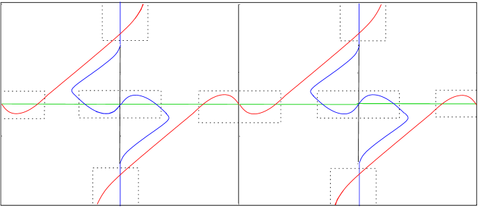
Figure 6. $\Gamma_{4}$ (red), $\Gamma_{2}$ (green), $\Gamma_{0}$ (blue) in $\mathbb{R}/2\pi\mathbb{Z}\times[-r,r]$.

Then we define $V_{4}\cap D(T^{*}L_{2})$, $V_{2}\cap D(T^{*}L_{2})$, $V_{0}\cap D(T^{*}L_{2})$ to be the unique 3 dimensional submanifolds in $D(T^{*}L_{2})$ whose intersection with every $D(T^{*}K_{ef})$ are given by $\Gamma_{4}$, $\Gamma_{4}$, $\Gamma_{4}$. Thus $V_{4}\cap D(T^{*}L_{2})$, $V_{2}\cap D(T^{*}L_{2})$, $V_{0}\cap D(T^{*}L_{2})$ are rotationally symmetric in the same sense as before. It is easy to see they are Lagrangian, and exact isotopic to $L_{4}\cap D(T^{*}L_{2})$, $L_{2}\cap D(T^{*}L_{2})$, $L_{0}\cap D(T^{*}L_{2})$.

What this deformation accomplishes is the following. There are still four triangles in $D(T^{*}K_{ef})$ with boundary on $V_{4}$, $V_{2}$, $V_{0}$, but now the vertices of these triangles do not lie on any of the four points $\pm e,\pm f\in K_{ef}\cap K_{2}^{\pm}$, where $P:T^{*}L_{2}\longrightarrow\mathbb{C}$ is singular. This ensures that $P$ can be trivialized over $T$ in the argument we discussed in §4c. (In addition $\Gamma_{4}$ and $\Gamma_{0}$ now intersect transversely, which will be useful when we compute Floer homology groups below.)

We complete the definition of $V_{0}$ by making it coincide with $L_{0}$ outside of $D(T^{*}L_{2})$. $V_{4}$ is extended outside of $D(T^{*}L_{2})$ in a similar way except we must take it to be the graph of an exact 1-form $df$ in $D(T^{*}L_{0})$ defined over $L_{0}\setminus U_{0}$ such that $df$ matches up with the part of $V_{4}$ near the boundary of $D(T^{*}L_{2})$; see §4e below for more details.

4e. Modification of $V_{4}$, $V_{2}$, $V_{0}$ (version III): Computing the Floer homology groups

Usually to compute Lagrangian Floer homology one takes an exact isotopy of one of the Lagrangians which makes it transverse to the other. We cannot do that because it would disrupt the symmetry of $V_{4}$, $V_{2}$, $V_{0}$ and ruin our argument in §4c. However, there is a variant of Floer homology (isomorphic to the usual one) which works for Lagrangians which only intersect cleanly (i.e. in Morse-Bott fashion); we call it Morse-Bott Floer homology.

The old Lagrangians $L_{4}$, $L_{2}$, $L_{0}$ did not even intersect cleanly, because $L_{4}$ and $L_{0}$ intersected in a closed manifold with boundary, namely $L_{0}$ minus a small neighborhood of $K_{0}$. (This was partially visible in figure 5: $\Gamma_{4}^{s}$ and $\Gamma_{0}^{s}$ intersect in four closed intervals.) However, the new Lagrangians $V_{4}\cap D(T^{*}L_{2})$, $V_{2}\cap D(T^{*}L_{2})$, $V_{0}\cap D(T^{*}L_{2})$ do intersect cleanly, because the curves $\Gamma_{4}$, $\Gamma_{2}$, $\Gamma_{0}$ intersect transversely.

It is useful to understand how the various intersection points between $\Gamma_{4}$, $\Gamma_{2}$, $\Gamma_{0}$ correspond to submanifolds in $D(T^{*}L_{2})$. First, consider the two dotted rectangles surrounding the six intersection points of $\Gamma_{0}$ (blue) and $\Gamma_{2}$ (green). The two midpoints correspond to the two points $\pm f\in K_{-}^{2}$. Thus, as $e$ and $f$ vary, the two midpoints together sweep out $K_{-}^{2}\cong S^{1}$. The four intersection points on either side of the two middle points in each rectangle together sweep out a torus, which is the boundary of a tubular neighborhood of $K_{-}^{2}$ in $V_{2}=L_{2}$, and we denote this torus by $\Sigma_{20}$. There is a similar story for the intersection points of $\Gamma_{4}$ (red) and $\Gamma_{2}$ (green), and we denote the torus there by $\Sigma_{42}$. The four intersection points of $\Gamma_{4}$ (red) and $\Gamma_{0}$ (blue) together sweep out a torus, denoted $\Sigma_{40}$, which can be viewed either as the boundary of $D_{s}(\nu^{*}K_{-}^{2})$ for a certain radius $s$, or as the boundary of a tubular neighborhood of $K_{0}$ in $L_{0}$ (recall $D(\nu^{*}K_{-}^{2})$ is identified with $U_{0}\subset L_{0}$, a tubular neighborhood of $K_{0}\subset L_{0}$).

Before discussing the computation of Floer homology groups we have to set up some regions in $M$ where we will localize the holomorphic strips which are involved in the calculation. First, consider the two horizontal dotted rectangles in figure 5 which surround the six intersection points of $\Gamma_{4}$ (red) and $\Gamma_{2}$ (green) (one of them is wrapped at the left and right edges of $\mathbb{R}/2\pi\mathbb{Z}\times[-1,1]$). The intersection of these two rectangles with $\Gamma_{2}$ yields two closed intervals in $\Gamma_{2}$. As $e$ and $f$ vary, these intervals sweep out a closed tubular neighborhood of $K_{+}^{2}$ in $V_{2}$, and we denote this by $N_{42}\subset V_{2}$. Now let $D(T^{*}N_{42})\subset D(T^{*}L_{2})$ denote a Weinstein neighborhood of $N_{42}$ which intersects each slice $D(T^{*}K_{ef})$ precisely in these two dotted rectangles. Note that inside the two rectangles we can view $\Gamma_{4}$ as the graph of two function over $\Gamma_{2}$. Corresponding to these functions there is an exact 1-form $df_{42}$ defined on $N_{42}$ such that the graph of $df_{42}$ in $D(T^{*}N_{42})$ is precisely $V_{4}\cap D(T^{*}N_{42})$. From the shape of $\Gamma_{4}$ we see that $f_{42}$ is a Morse-Bott function on $N_{42}$ with two critical components: it has a maximum at $K_{2}^{+}$ and a minimum at the torus $\Sigma_{42}$. In a similar way we define $D(T^{*}N_{20})$ which corresponds to the two dotted rectangles surrounding the intersection points of $\Gamma_{0}$ (blue) and $\Gamma_{2}$ (green). We define $df_{20}$ as before; from the shape of $\Gamma_{0}$ we can see $f_{20}$ is a Morse-Bott function on $N_{20}$ with two critical components: it has a minimum at $K_{2}^{-}$ and a maximum at the torus $\Sigma_{20}$.

Now take a look at the four partially formed vertical dotted rectangles surrounding the four intersection points of $\Gamma_{4}$ (red) and $\Gamma_{0}$ (blue); these rectangles intersect $\Gamma_{0}$ in four closed intervals. Together, these intervals correspond to an annular region in $L_{0}$ which surrounds $K_{0}$. Denote this region by $U_{0}\setminus\widetilde{U}_{0}$, where $\widetilde{U}_{0}\subset U_{0}$ is a smaller tubular neighborhood of $K_{0}$. We extend this region into $L_{0}$ by setting $N_{40}=L_{0}\setminus\widetilde{U}_{0}$. Then $N_{40}$ intersects $D(T^{*}K_{ef})\subset D(T^{*}L_{2})$ precisely in the four subintervals of $\Gamma_{0}$. Now take a Weinstein neighborhood $D(T^{*}N_{40})\subset D(T^{*}L_{0})$ which intersects $D(T^{*}K_{ef})\subset D(T^{*}L_{2})$ precisely in the four partially formed rectangles. To define $V_{4}$ outside of $D(T^{*}L_{2})$ more precisely, we take an Morse-Bott function $f_{40}:N_{40}\longrightarrow\mathbb{R}$ such that the graph of $df_{40}$ in $D(T^{*}N_{40})\cap D(T^{*}L_{2})$ agrees with $V_{4}\cap D(T^{*}N_{40})$. Thus, the part of the graph of $df_{40}$ in $D(T^{*}K_{ef})$ is represented by $\Gamma_{4}$ in the four partially formed rectangles. When we do the plumbing identification, these four rectangles in each slice $D(T^{*}K_{ef})$ are rotated by ninety degrees, via multiplication by $i$. (The complete sub-region of $D(T^{*}K_{ef})$ which is rotated is a neighborhood of $D(\nu^{*}K_{-}^{2})$, which would correspond to a rectangle around $\Gamma_{0}^{s}$, i.e. the two horizontal blue curves in figure 5.) After this rotation $\Gamma_{4}$ becomes the graph of a function defined over $\Gamma_{0}$ (the effect of $i$ or $-i$ is the same). Thus, $f_{40}$ is critical along $\Sigma_{40}$, and we assume that $f_{40}$ has isolated critical points aside from that. Then, from the shape of $\Gamma_{4}$ one can see $f_{40}$ has a maximum at $\Sigma_{40}$.

We are now ready to sketch how to compute the Floer homology groups $HF(V_{4},V_{2})$, $HF(V_{2},V_{0})$, and $HF(V_{4},V_{0})$. To do this calculation we modify $V_{4}$, $V_{2}$, $V_{0}$, but we do not change their basic shape. Namely, we replace $f_{40}$, $f_{42}$, $f_{20}$ by $\frac{1}{n}f_{40}$, $\frac{1}{n}f_{20}$, $\frac{1}{n}f_{42}$ for some large $n\geq 1$. Then we patch the graphs of $\frac{1}{n}df_{40}$, $\frac{1}{n}df_{42}$, $\frac{1}{n}df_{20}$ back into $V_{4}$, $V_{2}$, $V_{0}$ using some smooth bump function, and denote the result by $V_{4}^{n}$, $V_{2}^{n}$, $V_{0}^{n}$ (although $V_{2}^{n}=V_{2}=L_{2}$, as usual). Now let $J_{n}$ denote any sequence of almost complex structures on $M$ converging to some fixed $J$. Using a simple energy argument one can show that, for $n$ sufficiently large, the moduli space of $J_{n}$-holomorphic strips in $M$ with boundary on $(V_{4}^{n},V_{2}^{n})$ is completely contained in $D(T^{*}N_{42})$, and similarly for $(V_{4}^{n},V_{0}^{n})$, or $(V_{2}^{n},V_{0}^{n})$. Once this is known, we show there exist almost complex structures $J_{40}^{n}$, $J_{20}^{n}$, $J_{42}^{n}$ such that the above moduli spaces are in 1-1 correspondence with the gradient flow lines of $\frac{1}{n}f_{40}$, $\frac{1}{n}f_{20}$, $\frac{1}{n}f_{42}$ in $N_{40}$, $N_{20}$, $N_{42}$, when $n$ is large (this relies on Floer’s standard result of this type for closed manifolds). (As in Floer’s work, it follows from a linearized version of this correspondence that $J_{40}^{n}$, $J_{20}^{n}$, $J_{42}^{n}$ are regular for large $n$ as well.) Now, we fix an $n$ sufficiently large once for all and replace $V_{4}$, $V_{2}$, $V_{0}$ by $V_{4}^{n}$, $V_{2}^{n}$, $V_{0}^{n}$ and replace $f_{40}$, $f_{42}$, $f_{20}$ by $\frac{1}{n}f_{40}$, $\frac{1}{n}f_{42}$, $\frac{1}{n}f_{20}$, but we keep the old notation in both cases. Also we drop the $n$ from $J_{40}^{n}$, $J_{20}^{n}$, $J_{42}^{n}$ and denote them $J_{40}$, $J_{20}$, $J_{42}$. The above correspondence of moduli spaces yields an identification of $HF(V_{4},V_{2},J_{42})$ with $(H_{MB})_{*}(N_{42},f_{42})$, where the latter is a version of Morse homology for Morse-Bott functions called Morse-Bott homology. Similarly, $HF(V_{2},V_{0},J_{20})$ and $HF(V_{4},V_{0},J_{40})$ are isomorphic to $(H_{MB})_{*}(N_{20},f_{20})$ and $(H_{MB})_{*}(N_{40},f_{40})$. With our explicit Morse-Bott functions it is fairly easy to show that the Morse-Bott homology groups are isomorphic to $H_{*}(K_{+}^{2})$, $H_{*}(K_{-}^{2})$, and $H_{*}(L_{0}\setminus U_{0})$, respectively. Moreover, there are explicit generators and relations for the Morse-Bott homologies which match up with the ones for $H_{*}(K_{+}^{2})$, $H_{*}(K_{-}^{2})$, and $H_{*}(L_{0}\setminus U_{0})$ that we used in our computation of the flow category of $(N,f,g)$ in §3.

4f. Construction of $\widetilde{V}_{4}$, $\widetilde{V}_{2}$, $\widetilde{V}_{0}$ (version IV): Classification of holomorphic triangles in $M$, and a final correction to §4c

At the moment our Lagrangians $V_{4}$, $V_{2}$, $V_{0}$ are set up for computing the Floer homology groups. In this section we will deform them one last time, by exact isotopies, to new versions $\widetilde{V}_{4}$, $\widetilde{V}_{2}$, $\widetilde{V}_{0}$ (but with the same rough shape); these will allow us to describe the moduli space of $J$-holomorphic triangles in $M$ with boundary on $\widetilde{V}_{4}$, $\widetilde{V}_{2}$, $\widetilde{V}_{0}$, for a certain almost complex structure $J$. (In §4g below we will explain how to combine the results of this section and §4e.) There is also one last mistake to fix in §4c: In order to invoke the Riemann mapping theorem to construct the standard holomorphic triangles $w_{ef}$, it is necessary that the boundary arcs of the four triangles in figure 6 are real analytic. The new versions $\widetilde{V}_{4}$, $\widetilde{V}_{2}$, $\widetilde{V}_{0}$ will also remedy this problem. (Note that $\Gamma_{4}$, $\Gamma_{2}$, $\Gamma_{0}$ in figure 6 could not have triangles with real analytic edges because the edge corresponding to $\Gamma_{0}$ contains an interval in the region corresponding to $D(T^{*}N_{40})$.)

Fix a small connected compact neighborhood $U$ in $D(T^{*}L_{2})$ which contains all of the four triangles in $D(T^{*}K_{ef})$ in figure 5 for every $e,f$. Let $J_{\zeta}$, $\zeta\in V$ be any family of almost complex structures on $M$ such that $J_{\zeta}|_{U}=J_{\mathbb{C}}|_{U}$ for all $\zeta\in V$ (recall $V$ is the domain of our holomorphic triangles). First, we show that if the area of the four triangles in $D(T^{*}K_{ef})$ in figure 6 are sufficiently small then any $J$-holomorphic triangle must be contained in $U\subset D(T^{*}L_{2})$ (this follows from a relative version of the monotonicity lemma). Therefore, we deform $\Gamma_{4}$, $\Gamma_{2}$, $\Gamma_{0}$ to new versions $\widetilde{\Gamma}_{4}$, $\widetilde{\Gamma}_{2}$, $\widetilde{\Gamma}_{0}$ in such a way that these triangles become sufficiently small, as in figure 7.

Figure 7. $\widetilde{\Gamma}_{4}$ (red), $\widetilde{\Gamma}_{2}$ (green), $\widetilde{\Gamma}_{0}$ (blue) in $\mathbb{R}/2\pi\mathbb{Z}\times[-r,r]$.

In addition, we arrange that the the boundaries of the new triangles are real analytic. (In order to be real analytic the new $\widetilde{\Gamma}$’s must interpolate back to the old $\Gamma$’s away from the triangles; that is why there are small humps between $\widetilde{\Gamma}_{i}$ and $\Gamma_{i}$ next to each vertex of each triangle.) We denote the corresponding new $V_{4}$, $V_{2}$, $V_{0}$ by $\widetilde{V}_{4}$, $\widetilde{V}_{2}$, $\widetilde{V}_{0}$. Since every $J-$holomorphic triangle $w$ in $M$ with boundary on $\widetilde{V}_{4}$, $\widetilde{V}_{2}$, $\widetilde{V}_{0}$ lies in $U\subset D(T^{*}L_{2})$, and $J|_{U}=J_{\mathbb{C}}$, our classification result from §4c applies and we conclude that all such $w$ are equal to one of our standard ones $w_{ef}$. (For the monotonicity argument (see §8) we take a set $\widetilde{U}\subset U$, slightly smaller than $U$ and set $B=U\setminus\widetilde{U}$ to be an annular region surrounding the four triangles in $D(T^{*}K_{ef})$ in figure 5 for every $e,f$. Then $B$ acts as a barrier to holomorphic triangles in $U$ with large energy. It is important that $V_{i}\cap B=\widetilde{V}_{i}\cap B$ for every $i$; this can be arranged by making the small humps between $\widetilde{\Gamma}_{i}$ and $\Gamma_{i}$ in figure 7 at each vertex small enough.)

In addition, one can show that for any $J$ with $J|_{U}=J_{\mathbb{C}}|_{U}$ as above, $J$ is regular. This is proved in two steps. First one shows that the kernel of the linearized Cauchy-Riemann operator of $J$ has dimension 2; this proved by running through a version of the argument in §4c at the linearized level. Then one shows that the index of the operator is also equal to 2; this is proved using a gluing formula in the Morse-Bott setting which reduces the calculation to computing the Maslov index of a certain loop of Lagrangian tangent planes; the latter is fairly easy to compute because of the rotational symmetry of $\widetilde{V}_{4}$, $\widetilde{V}_{2}$, $\widetilde{V}_{0}$ in $D(T^{*}L_{2})$.

4g. Computing continuation maps; setting up to compute the triangle map $\mu_{2}$

In this section we combine the two calculations from §4e and §4f by inspecting the appropriate continuation maps. There are two issues we have to deal with: First, in the Floer homology calculation we used $(V_{4},V_{2},V_{0})$, whereas in the holomorphic triangle calculation we used $(\widetilde{V}_{4},\widetilde{V}_{2},\widetilde{V}_{0})$. Second, $J$ is not compatible with the almost complex structures we used in the Floer homology calculation, $J_{40}$, $J_{20}$, $J_{42}$. Here, compatible means that $J_{\zeta}$ is supposed to agree with $J_{40}$, $J_{20}$, or $J_{42}$, whenever $\zeta$ lies in a small neighborhood of one of the three corresponding boundary punctures of $V$ (but we have not arranged this to be so).

To address the second issue we pick some regular almost complex structures on $M$ for the Floer homology groups, say $\widetilde{J}_{40}$, $\widetilde{J}_{20}$, $\widetilde{J}_{42}$ such that $\widetilde{J}_{40}|_{U}$, $\widetilde{J}_{20}|_{U}$, $\widetilde{J}_{42}|_{U}$ are all equal to $J_{\mathbb{C}}|_{U}$ (it is easy to see we can pick them to be regular under this constraint for abstract reasons); then we pick our almost complex structure for the triangle calculation $J_{\zeta}$, $\zeta\in V$ also satisfying $J_{\zeta}|_{U}=J_{\mathbb{C}}|_{U}$ for all $\zeta$ and such that $J$ is compatible with $\widetilde{J}_{40}$, $\widetilde{J}_{20}$, $\widetilde{J}_{42}$. The condition $J|_{U}=J_{\mathbb{C}}|_{U}$ ensures that the whole discussion from §4f applies to $J$; in particular, $J$ is regular.

To address the first issue we take two functions $G,H:M\longrightarrow\mathbb{R}$ such that the Hamiltonian flows $\phi_{G}^{1},\phi_{H}^{1}:M\longrightarrow M$ satisfy $\phi^{1}_{G}(V_{4})=\widetilde{V}_{4}$ and $\phi_{H}^{1}(V_{4})=\widetilde{V}_{4}$. (Recall that $\widetilde{V}_{2}=V_{2}$.) Then, we have canonical isomorphisms

(4.18) $$HF(\widetilde{V}_{4},\widetilde{V}_{0},0,\widetilde{J}_{40})\cong HF(V_{4},V_{0},\{(G-H)\circ\phi_{G}^{t}\},\widetilde{J}_{40}^{*}),$$

$$HF(\widetilde{V}_{4},\widetilde{V}_{2},0,\widetilde{J}_{42})\cong HF(V_{4},V_{2},H,\widetilde{J}_{42}^{*}),$$

$$HF(\widetilde{V}_{2},\widetilde{V}_{0},0,\widetilde{J}_{20})\cong HF(V_{2},V_{0},\{-G\circ\phi^{t}_{G}\},\widetilde{J}_{20}^{*}).$$

These isomorphisms arise from a straight-forward equivalence between the underlying moduli spaces. For example, the middle one takes the form $u(s,t)\mapsto(\phi_{H}^{t})^{-1}(\phi_{H}^{1})^{-1}(u(s,t))$, where $u$ is a $\widetilde{J}_{42}$-holomorphic strip with boundary on $(\widetilde{V}_{4},\widetilde{V}_{2})$ $=$ $(\widetilde{V}_{4},V_{2})$. Above, $\widetilde{J}_{40}^{*}$, $\widetilde{J}_{20}^{*}$, $\widetilde{J}_{42}^{*}$ stand for the corresponding pull backs and push forwards of $\widetilde{J}_{40}$, $\widetilde{J}_{20}$, $\widetilde{J}_{42}$, for example $(\widetilde{J}_{40}^{*})_{t}=(\phi^{t}_{\{(G-H)\circ\phi^{t}_{G}\}})_{*}(\phi^{1}_{H})_{*}^{-1}(\widetilde{J}_{40})_{t}.$ (Each $J_{40}$, etc. and $\widetilde{J}_{40}$, etc. come in a family parameterized by $t\in[0,1]$, although we suppressed this earlier.) The precise formulas for the $\widetilde{J}^{*}$ are not relevant, however; the only thing that matters is that they are also regular; this is because of the natural equivalence between the moduli spaces (at the linearized level). Thus we are led to consider the continuation maps

$$\phi_{40}:HF(V_{4},V_{0},0,J_{40})\longrightarrow HF(V_{4},V_{0},\{(G-H)\circ\phi_{G}^{t}\},\widetilde{J}_{40}^{*}),$$

$$\phi_{42}:HF(V_{4},V_{2},0,J_{42})\longrightarrow HF(V_{4},V_{2},H,\widetilde{J}_{42}^{*}),$$

$$\phi_{20}:HF(V_{2},V_{0},0,J_{20})\longrightarrow HF(V_{2},V_{0},\{-G\circ\phi^{t}_{G}\},\widetilde{J}_{20}^{*}).$$

Recall near the end of §4e we mentioned there is a nice explicit set of generators and relations for $HF(V_{4},V_{2})$, $HF(V_{2},V_{0})$, and $HF(V_{4},V_{0})$ when we use the particular almost complex structures $J_{40}$, $J_{20}$, $J_{42}$. The important thing is they correspond exactly to the generators and relations we found for the flow category in §3. Therefore we want to show that the above continuation maps fix all the generators in this presentation (so that each continuation map in fact equals the identity on homology). We prove this by observing that each of the Hamiltonians, $(G-H)\circ\phi_{G}^{t}$, $H$, and $-G\circ\phi^{t}_{G}$, has either an absolute minimum or an absolute maximum along the relevant torus $\Sigma_{42}$, $\Sigma_{20}$, or $\Sigma_{40}$ (where all the generators live). Using this we can show that all $s-$dependent holomorphic strips $u$ (those which define the continuation map) which start and end at a point in $\Sigma_{42}$, $\Sigma_{20}$, or $\Sigma_{40}$ must be constant.

The groups $HF(\widetilde{V}_{4},\widetilde{V}_{0},\widetilde{J}_{40})$, $HF(\widetilde{V}_{2},\widetilde{V}_{0},\widetilde{J}_{20})$, $HF(\widetilde{V}_{4},\widetilde{V}_{2},\widetilde{J}_{42})$, are suitable for computing the triangle product because we can use our explicit classification of $J-$ holomorphic triangles in $M$, where $J$ is compatible with $\widetilde{J}_{40}$, $\widetilde{J}_{20}$, $\widetilde{J}_{42}$. We also know from what we’ve just done that these groups have generators and relations which correspond exactly to ones we found for the flow category. (One sees this by using the fact that the above continuation maps fix all the nice generators (and relations) on the left-hand side; then we use the natural isomorphisms from (4.18), which also fix all the generators.) Once we are in this situation it is fairly straight-forward to compute the triangle product (using our explicit knowledge of the holomorphic triangles) and compare that to the product in the flow category generator by generator; in fact the computations are completely parallel. We will not try to summarize that calculation in our present technical set up (this is presented fairly clearly in the proof of Theorem 10.1). Instead, we will present in §4h below an intuitive argument which explains why we expect the triangle product $\mu_{2}$, and the flow category product, $\mu^{Flow}$, to be the same. In many ways this argument parallels the actual argument, but hopefully the main ideas are less obscured by technicalities.

4h. Intuitive sketch of the isomorphism in Theorem $B$

In this section we will ignore all the technical difficulties that we have dealt with up until now and work with the simplest version of the Lagrangians $L_{0}$, $L_{2}$, $L_{4}$. Our goal is to illustrate the essential idea of the calculation of the triangle product with the technical aspects stripped away. Along the way we will assume various things which are not quite true as stated, but it should be clear from the above that it is possible to tweak the Lagrangians so that the statements transform into new ones which are true, and are essentially the same as the old ones. In this sense the argument is morally correct; in any case it should be a useful guide to the proof of Theorem 10.1, which presents a technically correct argument.

Let us return to the more general case where $N$ has any number of 2-handles, so that we that can compare more directly with the flow category calculation in §3. Then, the handle-decomposition of $N$ gives rise to $k$ framed knots $K_{1},\ldots,K_{k}\subset S^{3}$, one for each 2-handle. Let $L_{0}=S^{3}$, and take $k$ parameterizations of tubular neighborhoods of $K_{1},\ldots,K_{k}\subset L_{0}$, which are determined up to isotopy, say $\phi_{j}:S^{1}\times D^{2}\longrightarrow L_{0}$, $j=1,\ldots,k$. Now take $k$ additional copies of $S^{3}$, denoted $L_{2}^{j}$, $j=1,\ldots,k$. As before we have two natural unknots $K_{\pm}^{j}\subset L_{2}^{j}$ for each $j$, and for each $e\in K_{+}^{j}$, $f\in K_{-}^{j}$, we have the great circle $K_{ef}^{j}\subset L_{2}^{j}$. We construct $M$ by taking the disk bundle $D(T^{*}L_{0})$ and plumbing on each of the disk bundles $D(T^{*}L_{2}^{j})$ along the knots $K_{j}$. Here $D(\nu^{*}K_{-}^{j})\cong S^{1}\times D^{2}$ will be identified with a tubular neighborhood of $K_{j}$ in $L_{0}$, say $U_{0}^{j}\subset L_{0}$ using the map $\phi_{j}$. The last Lagrangian $L_{4}$ is defined by doing Lagrangian surgery of $L_{0}$ with each of the $L_{2}^{j}$ (in the same way $L_{4}$ was defined before).

We make two main assumptions. First, we assume that inside each $D(T^{*}L_{2}^{j})$, we have our standard holomorphic triangles $w_{ef}^{j}$, one for each $e\in K_{+}^{j}$, $f\in K_{-}^{j}$, and we assume that every holomorphic triangle in $M$ coincides with one of these $w_{ef}^{j}$. Second, we assume we have identifications

$$HF(L_{4},L_{2}^{j})\cong H_{*}(L_{4}\cap L_{2}^{j})\cong H_{*}(K_{2}^{j}),$$

$$HF(L_{2}^{j},L_{0})\cong H_{*}(L_{2}^{j}\cap L_{0})\cong H_{*}(K_{j}),$$

$$HF(L_{4},L_{0})\cong H_{*}(L_{4}\cap L_{0})\cong H_{*}(L_{0}\setminus(\cup_{j}U_{0}^{j})).$$

In this way the morphism spaces in $H(Fuk^{\rightarrow}(M;L_{4},\{L_{2}^{j}\},L_{0}))$ are identified with those in $Flow(N,f,g)$. Recall that $w_{ef}^{j}$ is the unique holomorphic triangle in $D(T^{*}K_{ef}^{j})$ with two of its vertices at $e$, $f$. The final vertex of $w_{ef}^{j}$ determines a third point, which we denote $\psi_{j}(e,f)\in D(T^{*}K_{ef})$; it lies in the sphere conormal bundle $S(\nu^{*}K_{-}^{j})\subset D(T^{*}L_{2}^{j})$, which is a torus, since $\nu^{*}K_{-}^{j}\cong S^{1}\times\mathbb{R}^{2}$. Now, $S(\nu^{*}K_{-}^{j})$ is identified by $\phi_{j}$ with the boundary of a smaller neighborhood $U_{j}\subset U_{0}^{j}$ of $K_{j}$ in $L_{0}$.

Let us choose some generators for $H_{*}(K_{+}^{j}\times K_{-}^{j})$, $H_{*}(S(\nu^{*}K_{-}^{j}))$, and $H_{*}(L_{0}\setminus(\cup_{j}U_{0}^{j}))$. We choose notation similar to that used in §3. For $H_{*}(K_{+}^{j}\times K_{-}^{j})$, fix $r_{\pm}^{j}\in K_{+}^{j}$ and take the generators

$$T_{+}^{j}=[K_{+}^{j}\times K_{-}^{j}],\,\,\lambda_{+}^{j}=[r_{+}^{j}\times K_{-}^{j}],\,\,\mu_{+}^{j}=[K_{+}^{j}\times r_{-}^{j}],\,\,s_{+}^{j}=[r_{+}^{j}\times r_{-}^{j}].$$

For $H_{*}(S(\nu^{*}K_{-}^{j}))$, we identify $S(\nu^{*}K_{-}^{j})=K_{-}^{j}\times K_{+}^{j}$ (this is natural because a point in $K_{+}^{j}$ determines a direction in the normal bundle of $K_{-}^{j}$) and take the generators

$$T_{-}^{j}=[K_{-}^{j}\times K_{+}^{j}],\,\,\lambda_{-}^{j}=[K_{-}^{j}\times r_{+}^{j}],\,\,\mu_{-}^{j}=[r_{-}^{j}\times K_{+}^{j}],\,\,s_{-}^{j}=[r_{-}^{j}\times r_{+}^{j}].$$

Now $H_{*}(L_{0}\setminus(\cup_{j}U_{0}^{j}))$ is generated by cycles in $\partial U_{j}$ (where $U_{j}\subset U_{0}^{j}$ and $\phi_{j}(S(\nu^{*}K_{-}^{j}))$ $=$ $\partial U_{j}$). Let $q_{j}\in\partial U_{j}$ and let $\lambda_{j},\mu_{j}\subset H_{1}(\partial U_{j})$ be represented by circles with $\ell(\lambda_{j},K_{j})=0$ and $\ell k(\mu_{j},K_{j})=1$. Then $H_{*}(L_{0}\setminus(\cup_{j}U_{0}^{j}))$ is generated by $[\partial U_{j}],$ $\lambda_{j},$ $\mu_{j},$ and $[q_{j}]$, with the same relations (3.15) from §3.

Here is an intuitive way to think about the triangle product

$$\mu_{2}:HF(L_{4},L_{2}^{j})\otimes HF(L_{2}^{j},L_{0})\longrightarrow HF(L_{4},L_{0})$$

in terms of the geometric cycles above. Take a pair of cycles on the right hand side, which we represent by submanifolds $C_{+}^{j}$, $C_{-}^{j}$ in $K_{+}^{j}$, $K_{-}^{j}$ (so $C_{\pm}^{j}=K_{j}^{\pm}$ or $C_{\pm}^{j}=r_{j}^{\pm}$). Now, as a first step, restrict attention to $D(T^{*}L_{2}^{j})$ and consider the cycle in $S(\nu^{*}K_{-}^{j})$ that gets swept out by the points $\psi_{j}(e,f)$, as $(e,f)$ range over $C_{+}^{j}\times C_{-}^{j}$, and denote this by $\mu_{2}|_{D(T^{*}L_{2}^{j})}(C_{+}^{j},C_{-}^{j})$. Next, $S(\nu^{*}K_{-}^{j})$ is identified by the framing $\phi_{j}$ with $\partial U_{j}$, and in this way we get a cycle in $\partial U_{j}$ which is $\mu_{2}(C_{+}^{j},C_{-}^{j})=\phi_{j}(\mu_{2}|_{D(T^{*}L_{2}^{j})}(C_{+}^{j},C_{-}^{j}))$.

In the first step above, it is easy to see that the restricted triangle product

$$\widetilde{\mu}_{2}=\mu_{2}|_{D(T^{*}L_{2}^{j})}:H_{*}(K_{+}^{j})\otimes H_{*}(K_{-}^{j})\longrightarrow H_{*}(S(\nu^{*}K_{-}^{j}))$$

satisfies $\widetilde{\mu}_{2}(T_{+}^{j})=T_{-}^{j}$, $\widetilde{\mu}_{2}(\lambda_{+}^{j})=\mu_{-}^{j}$, $\widetilde{\mu}_{2}(\mu_{+}^{j})=\lambda_{-}^{j}$, $\widetilde{\mu}_{2}(s_{+}^{j})=s_{-}^{j}$. These are analogous to the relations (3.17) satisfied by the flow map $\Phi$ in the fixed handle $H_{j}$ in §3. In the second step, one composes $\widetilde{\mu}_{2}$ with the map on homology induced by $\phi_{j}:S(\nu^{*}K_{-}^{j})\longrightarrow\partial U_{j}$ and the inclusion $\partial U_{j}\subset L_{0}\setminus(\cup_{j}U_{0}^{j})$,

$$(\phi_{j})_{*}:H_{*}(S(\nu^{*}K_{-}^{j}))\longrightarrow H_{*}(L_{0}\setminus(\cup_{j}U_{0}^{j})).$$

As in (3.16), we have

$$(\phi_{j})_{*}(\lambda_{-}^{j})=\lambda_{j}+m_{j}\mu_{j},\,(\phi_{j})_{*}(\mu_{-}^{j})=\mu_{j}.$$

Combining these we have, for example,

$$\mu_{2}([K_{+}^{j}]\otimes[r_{-}^{j}])=(\phi_{j})_{*}(\widetilde{\mu}_{2}(\mu_{+}^{j}))=(\phi_{j})_{*}(\lambda_{-}^{j})=\lambda_{j}+m_{j}\mu_{j},\text{ while }$$

$$\mu^{Flow}([K_{+}^{j}]\otimes[p_{-}^{j}])=(\phi_{j})_{*}(\Phi(\mu_{+}))=(\phi_{j})_{*}(\lambda_{-})=\lambda_{j}+m_{j}\mu_{j}.$$

Notice that the answers agree, but also the calculations are parallel.

4i. The case general case $\textup{dim}N=2n$, when $f$ has critical values $0,n,2n$

In this section we briefly summarize how things work in an arbitrary dimension $\textup{dim}N=2n$. The handle decomposition of $N$ corresponding to $(f,g)$ is determined by $k$ framed $(n-1)$-spheres in a $(2n-1)$-sphere, $K_{j}\subset S^{2n-1}$, $j=1,\ldots,k$. The flow category calculation is much the same, and we omit that discussion. To construct $M$ we take $L_{0}=S^{2n-1}$ and $L_{n}^{j}=S^{2n-1}$, $j=1,\ldots,k$. In $L_{0}$ we have the framed spheres $K_{j}$ and inside $L_{n}^{j}$ we have the two $(n-1)$-spheres with obvious framings

$$K_{+}^{j}=\{(u_{1},\ldots,u_{n},0,\ldots,0):\Sigma u_{j}^{2}=1\},K_{-}^{j}=\{(0,\ldots,0,u_{n+1},\ldots,u_{2n}):\Sigma u_{j}^{2}=1\}.$$

We plumb as before; and $L_{4}$ is defined in the same way, by applying the time $\pi/2$ Hamiltonian flow to $D(\nu^{*}K_{-}^{j})$. The classification of holomorphic triangles in $M$ works as before: For each $e\in K_{+}^{j}$, $f\in K_{-}^{j}$ we have the great circle $K_{ef}^{j}\subset L_{2}^{j}$ and there is a unique holomorphic triangle $w_{ef}^{j}$ in $D(T^{*}K_{ef}^{j})\subset D(T^{*}L_{2}^{j})$ with each of its vertices determined by $(e,f)$; and these are the only holomorphic triangles in $M$. Then the identification of the two categories is done in the same way as the sketch above. (One thing to note is that we do not need to explicitly know the relations (3.15). Indeed, whatever these relations are, they show up abstractly in the calculation of the flow category and the directed Fukaya category in exactly the same way.)

5. Constructing $M$ (the fiber)

In §5a we give a precise treatment of the plumbing construction sketched in §4a. It turns out that the plumbing, which we denote $M_{0}$, has boundary which is not smooth. Therefore, in §5b we construct a slightly bigger space $M$ which is obtained from $M_{0}$ by smoothing the boundary, so that $M$ has convex, contact type boundary.

5a. Plumbing

Let $(N,f,g)$ be as in §3. Denote the critical points of $f$ by $x_{0},x_{2}^{j},x_{4},$ $j=1,\ldots,k$. Here the index of the critical point is given by the subscript. Let

$$L_{0}=f^{-1}(1)\cong S^{3},\text{ and }L_{2}^{j}=S^{3},\,j=1\ldots k.$$

Now define

$$K_{j}=U(x_{2}^{j})\cap f^{-1}(1)\subset L_{0},$$

and let

$$\phi_{j}:S^{1}\times\mathbb{R}^{2}\longrightarrow L_{0}$$

denote a parameterization of a tubular neighborhood of $K_{j}$ determined by $(f,g)$ up to isotopy. Let $K_{-}^{j},K_{+}^{j}\subset L_{2}^{j}$, denote the two unknots

$$K_{-}^{j}=\{(0,0,x_{3},x_{4})|x_{3}^{2}+x_{4}^{2}=1\}\text{ and }K_{+}^{j}=\{(x_{1},x_{2},0,0)|x_{1}^{2}+x_{2}^{2}=1\}.$$

We specify a parameterization of a tubular neighborhood of $K_{-}^{j}$ in $L_{2}^{j}$ as follows. First take the obvious identification of $S^{1}\times\mathbb{R}^{2}$ with the normal bundle of $K_{-}^{j}$ in $TS^{3}$. Then, using this identification, we let

$$\phi_{-}^{j}:S^{1}\times D^{2}_{\pi/3}\longrightarrow L_{0},$$

be the map given by geodesic coordinates with respect to the round metric on $S^{3}$. (Here we take $\pi/3<\pi/2$ so that $\phi_{-}^{j}$ is an embedding.) For use later on we define $\phi_{+}^{j}:S^{1}\times D^{2}_{\pi/3}\longrightarrow L_{2}^{j}$ for $K_{+}^{j}$ in the same way.

We start with the disjoint union of the disk bundles $D(T^{*}L_{0})$ and $D(T^{*}L_{2}^{j})$, $j=1,\ldots,k$. Then for each $j$ we glue a neighborhood of $K_{j}\subset D(T^{*}L_{0})$ to a neighborhood of $K_{-}^{j}\subset D(T^{*}L_{2}^{j})$. Each neighborhood can be symplectically identified with a neighborhood of $S^{1}\times\{0\}$ in $T^{*}S^{1}\times T^{*}\mathbb{R}^{2}\cong T^{*}S^{1}\times\mathbb{C}^{2}$ and each gluing map is of the form $id_{T^{*}S^{1}}\times m_{i}$, where $m_{i}$ is multiplication by $i$ on $\mathbb{C}^{2}$.

To be more precise, we choose some convenient metrics with which to form the disk bundles $D(T^{*}L_{0})$ and $D(T^{*}L_{2}^{j})$, and we fix the radii. Let $g_{2}$ be a Riemannian metric on $\cup_{j}L_{2}^{j}$ such that,

$$g_{2}=(\phi_{-}^{j})_{*}(g_{S^{1}}\times g_{\mathbb{R}^{2}})\text{ on }\phi_{-}^{j}(S^{1}\times D^{2}_{\pi/3}),$$

$$g_{2}=(\phi_{+}^{j})_{*}(g_{S^{1}}\times g_{\mathbb{R}^{2}})\text{ on }\phi_{+}^{j}(S^{1}\times D^{2}_{\pi/3}),$$

and outside of a small neighborhood of $\phi_{-}^{j}(S^{1}\times D^{2}_{\pi/3})\cup\phi_{+}^{j}(S^{1}\times D^{2}_{\pi/3})$, $g_{2}$ is the round metric $g_{S^{3}}$. On the intermediate region we linearly interpolate between $(\phi_{j}^{\pm})_{*}(g_{S^{1}}\times g_{\mathbb{R}^{2}})$ and $g_{S^{3}}$ using some cut-off function. Let $g_{0}$ be a Riemannian metric on $L_{0}$, such that

$$g_{0}=(\phi_{j})_{*}(g_{S^{1}}\times g_{\mathbb{R}^{2}})\text{ on }\phi_{j}(S^{1}\times\mathbb{R}^{2}),$$

and outside of $\phi_{j}(S^{1}\times\mathbb{R}^{2})$, $g_{0}$ is arbitrary. Now, fix $r,R>0$ such that

$$0<r<R<\pi/3.$$

$R$ will be the radius of $D(T^{*}L_{0})=D_{r}^{g_{0}}(T^{*}L_{0})$ and $r$ will be the radius of $D(T^{*}L_{2}^{j})=D_{r}^{g_{2}}(T^{*}L_{2}^{j})$.

Now $\phi_{-}^{j},\phi_{j}$ respectively give rise to exact symplectic identifications

$$\rho_{-}^{j}:T^{*}(S^{1})\times T^{*}(D^{2}_{r})\longrightarrow T^{*}(\phi_{-}^{j}(S^{1}\times D^{2}_{r})),$$

$$\rho_{j}:T^{*}(S^{1})\times T^{*}(\mathbb{R}^{2})\longrightarrow T^{*}(\phi_{j}(S^{1}\times\mathbb{R}^{2})).$$

We take two sets of coordinates on $T^{*}(S^{1})\times T^{*}(\mathbb{R}^{2})$

$$q\in S^{1},p\in T^{*}_{q}S^{1},x\in\mathbb{R}^{2},y\in T^{*}_{x}\mathbb{R}^{2},$$

$$\widetilde{q}\in S^{1},\widetilde{p}\in T^{*}_{\widetilde{q}}S^{1},\widetilde{x}\in\mathbb{R}^{2},\widetilde{y}\in T^{*}_{\widetilde{x}}\mathbb{R}^{2}.$$

To do the plumbing we will identify the following two regions in $D_{R}^{g_{0}}(T^{*}L_{0})$ and $D_{r}^{g_{2}}(T^{*}L_{2}^{j})$ respectively. Let

$$U_{0}^{j}=\rho_{j}(\{((q,p),(x,y)):|p|_{S^{1}}^{2}+|y|^{2}_{\mathbb{R}^{2}}\leq R^{2},|x|_{\mathbb{R}^{2}}^{2}+|p|_{S^{1}}^{2}\leq r^{2}\}),$$

$$U_{2}^{j}=\rho_{-}^{j}(\{((\widetilde{q},\widetilde{p}),(\widetilde{x},\widetilde{y})):|\widetilde{p}|_{S^{1}}^{2}+|\widetilde{y}|^{2}_{\mathbb{R}^{2}}\leq r^{2},|\widetilde{p}|_{S^{1}}^{2}+|\widetilde{x}|^{2}_{\mathbb{R}^{2}}\leq R^{2}\}).$$

Note that, since $|x|^{2}_{\mathbb{R}^{2}}\leq|p|_{S^{1}}^{2}+|x|^{2}_{\mathbb{R}^{2}}\leq r^{2}<(\pi/3)^{2}$, $g_{0}$ agrees with the metric used in $U_{0}^{j}$, and so indeed have

$$U_{0}^{j}\subset D_{R}^{g_{0}}(T^{*}L_{0})\text{ and, similarly, }U_{2}^{j}\subset D_{R}^{g_{2}}(T^{*}L_{2}^{j}).$$

Define a symplectomorphism

$$\tau^{j}:U_{2}^{j}\longrightarrow U_{0}^{j}\text{ by }(\widetilde{q},\widetilde{p},\widetilde{x},\widetilde{y})\mapsto(q,p,-y,x).$$

Define $M_{0}$ by gluing $D_{R}^{g_{0}}(T^{*}L_{0})$ and $D_{r}^{g_{2}}(T^{*}L_{2}^{j})$ along the subsets $U_{0}^{j}$, $U_{2}^{j}$ for each $j=1,\ldots,k$ using $\tau^{j}$. We call this a plumbing (along $K_{j},K_{-}^{j}$) and denote it

$$M_{0}=D_{R}^{g_{0}}(T^{*}L_{0})\boxplus_{\,j=1}^{\,j=k}D_{r}^{g_{2}}(T^{*}L_{2}^{j}).$$

Lemma 5.1.

The interior of $M_{0}$ is smooth and has an exact symplectic structure which agrees with the standard symplectic structures on $D_{R}^{g_{0}}(T^{*}L_{0})$ and $D_{r}^{g_{2}}(T^{*}L_{j}^{2})$, $j=1,\ldots,k$.

Proof.

The main issue is topological: We must prove that $U_{0}^{j}$ and $U_{2}^{j}$ reach the boundary of $D_{R}^{g_{0}}(T^{*}L_{0})$ and $D_{r}^{g_{2}}(T^{*}L_{j}^{2})$ respectively. (To see what could go wrong imagine gluing $\mathbb{R}\times[-1,1]$ to $\mathbb{R}\times[-1,1]$ along $[-1/2,1/2]\times[-1/2,1/2]$, using the map $(x,y)\mapsto(-y,x)$.) The boundary of $U_{0}^{j}$ has two parts, which we will call horizontal and vertical. The horizontal part is

$$\partial_{h}U_{0}^{j}=\{((q,p),(x,y)):|p|_{S^{1}}^{2}+|y|^{2}_{\mathbb{R}^{2}}=R^{2},|x|_{\mathbb{R}^{2}}^{2}+|p|\\ \newline _{S^{1}}^{2}\leq r^{2}\},$$

and the vertical part is

$$\partial_{v}U_{0}^{j}=\{((q,p),(x,y)):|p|_{S^{1}}^{2}+|y|^{2}_{\mathbb{R}^{2}}\leq R^{2},|x|_{\mathbb{R}^{2}}^{2}+|p|_{S^{1}}^{2}=r^{2}\},$$

Similarly we have $\partial_{h}U_{2}^{j}$ and $\partial_{v}U_{2}^{j}$. Note that $\tau^{j}$ maps $\partial_{h}U_{2}^{j}$ to $\partial_{v}U_{0}^{j}$ and $\partial_{v}U_{2}^{j}$ to $\partial_{h}U_{0}^{j}$. Now, since $|x|^{2}_{\mathbb{R}^{2}}\leq|p|_{S^{1}}^{2}+|x|^{2}_{\mathbb{R}^{2}}\leq r^{2}<(\pi/3)^{2}$, $g_{0}$ agrees with the metric used in $U_{0}^{j}$, and so we have

$$\partial_{h}U_{0}^{j}\subset S_{R}^{g_{0}}(T^{*}L_{0}).$$

Similarly $\partial_{h}U_{2}^{j}\subset S_{r}^{g_{2}}(T^{*}L_{2}^{j}).$ This shows that $U_{0}^{j}$ and $U_{2}^{j}$ each reach the boundary of $D_{R}^{g_{0}}(T^{*}L_{0})$ and $D_{r}^{g_{2}}(T^{*}L_{j}^{2})$ respectively, and so $\textup{Int\,}(M_{0})$ is locally Euclidean. It is smooth and symplectic since $\tau^{j}$ is, and the Mayer-Vietoris sequence in de Rham cohomology shows the symplectic form is exact. ∎

Let us denote the symplectic structure on $M_{0}$ by $\omega_{0}$. We fix a primitive $\theta_{0}$, with $\omega_{0}=d\theta_{0}$.

5b. Handle attachments

The simplest example of a plumbing is obtained by gluing $\mathbb{R}\times[-1,1]$ to $\mathbb{R}\times[-1,1]$ along $[-1,1]\times[-1,1]$ using $(x,y)\mapsto(-y,x)$. This shows $M_{0}$ is not an exact symplectic manifold with corners in the sense of [S08, §7a]: it has obtuse corners, and the combined convexity of $S_{R}^{g_{0}}(T^{*}L_{0})$ and $S_{r}^{g_{2}}(T^{*}L_{2}^{j})$ are not enough to prevent holomorphic curves from hitting a corner. To remedy this we have an alternative construction from [J09B] (see also [J09A]). There we construct $M$ by attaching $k$ Morse-Bott type handles to $D(T^{*}L_{0})$ in the style of [W91], one for each $j=1,\ldots,k$. Each handle $H_{j}$ is diffeomorphic to $D(T^{*}(S^{1}\times D^{2}))$, where we think of $S^{1}$ as a critical manifold (which corresponds to $K_{+}^{j}$) and $S^{1}\times D^{2}$ as its unstable manifold. To attach $H_{j}$ we identify $D(T^{*}(S^{1}\times D^{2}))|(S^{1}\times\partial D^{2})$ with a neighborhood of $S(\nu^{*}K_{j})$ in $S(T^{*}L_{0})$ so that $S^{1}\times D^{2}$ and $D(\nu^{*}K_{j})$ together form a Lagrangian 3-sphere $\widetilde{L}_{2}^{j}$. The following lemma summarizes the relation between $M_{0}$ and $M$.

Lemma 5.2 ([J09B]).

There is an exact symplectic manifold $(M,\omega,\theta)$ with smooth, convex, contact type boundary, together with an exact symplectic embedding

$$j:(M_{0},\omega_{0},\theta_{0})\longrightarrow(M,\omega,\theta).$$

such that $j(L_{2}^{j})=\widetilde{L}_{2}^{j}$ and $j|L_{0}$ is the obvious embedding. See figure 8. $\square$

We mention also that $M$ and $M_{0}$ are homeomorphic, via a retraction $M\longrightarrow j(M_{0})$, but we will not need this.

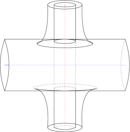
Figure 8. Schematic of $M_{0}$ (inner) and $M$ (outer) near the plumbing region.

6. Constructing $V_{4},V_{2}^{j},V_{0}$ (the vanishing spheres)

In this section we construct the vanishing spheres $V_{4},V_{2}^{j},V_{0}$ in $M_{0}$; these correspond to version II of the vanishing spheres in §4d. We will only have a few things to add beyond the description there.

We regard $T^{*}L_{2}^{j}=T^{*}S^{3}$ as $\{(u,v)\in\mathbb{R}^{4}\times\mathbb{R}^{4}:|u|=1,u\cdot v=0\}$, with the restriction of the symplectic structure $\Sigma_{j}dv_{j}\wedge du_{j}$ from $\mathbb{R}^{8}$. Recall from §5 we have the two standard unknots $K_{+}^{j}$, $K_{-}^{j}$ in $L_{2}^{j}$. For each $e\in K_{+}^{j}$, $f\in K_{-}^{j}$, we have the great circle through $e,f$ in $L_{2}^{j}$, denoted $K_{ef}^{j}=\{(\cos(\theta)e,\sin(\theta)f):\theta\in\mathbb{R}/2\pi\mathbb{Z}\}$. (Note that $K_{ef}^{j}=K_{\pm e,\pm f}^{j}$.) We also embed $T^{*}K_{ef}^{j}$ in $T^{*}L_{2}^{j}$ as

$$T^{*}K_{ef}^{j}=\{((\cos(\theta)e,\sin(\theta)f),\lambda(-\sin(\theta)e,\cos(\theta)f):\theta\in\mathbb{R}/2\pi\mathbb{Z},\lambda\in\mathbb{R}\}.$$

For each $e\in K_{+}^{j}$, $f\in K_{-}^{j}$ we fix an identification

$$\sigma_{ef}^{j}:(\mathbb{R}/2\pi\mathbb{Z})\times\mathbb{R}\longrightarrow T^{*}K_{ef},\phantom{2}\sigma_{ef}^{j}(\theta,\lambda)=(\cos(\theta)e,\sin(\theta)f),\lambda(-\sin(\theta)e,\cos(\theta)f).$$

Note that $\sigma_{ef}^{j}$ maps $(\mathbb{R}/2\pi\mathbb{Z})\times[-r,r]$ onto $D_{r}^{g_{S^{3}}}(T^{*}K_{ef}^{j})$, where $g_{S^{3}}$ is the round metric. But in fact $D_{r}^{g_{S^{3}}}(T^{*}K_{ef}^{j})=D_{r}^{g_{2}}(T^{*}K_{ef}^{j})$, because $g_{S^{3}}(v,v)=g_{2}(v,v)$ for any $v\in T^{*}K_{ef}^{j}$. (Indeed, it is easy to check that $g_{S^{3}}$ and $(\phi_{-}^{j})_{*}(g_{S^{1}}\times g_{\mathbb{R}^{2}})$ agree on $T^{*}K_{ef}^{j}$ in a neighborhood of $K_{-}^{j}$, and then it follows that the equality holds on all of $S^{3}$ because $g_{2}$ is defined by linearly interpolating between $g_{S^{3}}$ and $(\phi_{-}^{j})_{*}(g_{S^{1}}\times g_{\mathbb{R}^{2}})$.) From now on we will omit the metric and radius from the notation in $D(T^{*}L_{2}^{j})=D_{r}^{g_{2}}(T^{*}L_{2}^{j})$ and $D(T^{*}L_{0})=D_{R}^{g_{0}}(T^{*}L_{0})$.

Let $\Gamma_{0}$,$\Gamma_{2}$,$\Gamma_{4}$ be the three curves as in figure 6.

Figure 9. $\Gamma_{4}$ (red), $\Gamma_{2}$ (green), $\Gamma_{0}$ (blue) in $\mathbb{R}/2\pi\mathbb{Z}\times[-r,r]$.

We define some 3 dimensional submanifolds (possibly with boundary)

$$W_{0}^{j},W_{2}^{j},W_{4}^{j}\subset D(T^{*}L_{2}^{j}),\text{ by }W_{i}^{j}=\cup_{e,f}\,\sigma_{ef}^{j}(\Gamma_{i}),\,i=0,2,4.$$

This means that $W_{0}^{j},W_{2}^{j},W_{4}^{j}$ are rotationally symmetric in the sense that the intersection of $W_{0}^{j}$, $W_{2}^{j}$, $W_{4}^{j}$ with any slice $D(T^{*}K_{ef}^{j})$, is given by figure 6. We define the parts of $V_{0},V_{2}^{j},V_{4}\subset M_{0}$ which lie in $D(T^{*}L_{2}^{j})$ by

$$V_{0}\cap D(T^{*}L_{2}^{j})=W_{0}^{j},\,V_{2}^{j}\cap D(T^{*}L_{2}^{j})=W_{2}^{j},\,V_{4}\cap D(T^{*}L_{2}^{j})=W_{4}^{j}.$$

Note that $V_{2}^{j}=L_{2}^{j}=W_{2}^{j}$. It is easy to see that $W_{0}^{j}$, $W_{2}^{j}$, $W_{4}^{j}$ are Lagrangian. Note that $\Gamma_{0}$, $\Gamma_{2}$, $\Gamma_{4}$ are exact isotopic to the three corresponding curves $\Gamma_{0}^{s}$, $\Gamma_{2}^{s}$, $\Gamma_{4}^{s}$ in figure 5 in §4b, since the signed area between $\Gamma_{i}$ and $\Gamma_{i}^{s}$ is zero. From this it is not it difficult to show that $W_{0}^{j}$ and $W_{4}^{j}$ are exact isotopic to $D(\nu^{*}K_{-}^{j})$ and $D(\nu^{*}K_{+}^{j})$, respectively.

We define $V_{0}\subset M_{0}$ as the union of $L_{0}\setminus\big{(}\cup_{j=1}^{j=k}\phi_{j}(S^{1}\times\textup{Int\,}(D^{2}_{r}))\big{)}$ and $\cup_{j=1}^{j=k}\,W_{0}^{j}$; here $D^{2}_{r}$ is the closed disk of radius $r$. (Notice that these two pieces match up, since $W_{0}^{j}$ coincides with $D_{r}(\nu^{*}K_{-}^{j})=\phi_{j}(S^{1}\times D^{2}_{r})$ near the boundary of $D(T^{*}L_{2}^{j})$.) Then $V_{0}$ is exact isotopic to $L_{0}$, since $W_{0}^{j}$ is exact isotopic to $D(\nu^{*}K_{-}^{j})$.

We give a rough definition of $V_{4}$ and leave more precise details to §7a below. First take the graph of an exact one-form $df$ in $D(T^{*}L_{0})$ defined on $L_{0}\setminus\big{(}\cup_{j=1}^{j=k}\phi_{j}(S^{1}\times\textup{Int\,}(D^{2}_{r}))\big{)}$ such that the graph of $df$ matches up with $\cup_{j=1}^{j=k}\,W_{4}^{j}$. (In §7a below we will specify $df$ more precisely and denote it $df_{40}$.) Now define $V_{4}\subset M_{0}$ as the union of the graph of $df$ and $\cup_{j=1}^{j=k}\,W_{4}^{j}$. Then, $V_{4}$ is an exact Lagrangian sphere because $df$ is exact isotopic to $L_{0}\setminus\big{(}\cup_{j=1}^{j=k}\phi_{j}(S^{1}\times\textup{Int\,}(D^{2}_{r}))\big{)}$ and $W_{4}^{j}$ is exact isotopic to $D_{r}(\nu^{*}K_{+}^{j})\cong S^{1}\times D^{2}_{r}$. This also shows $V_{4}$ is diffeomorphic to the result of doing surgery on $L_{0}$ along the framed link $\cup_{j}K_{j}$. Related to this, $V_{4}$ is exact isotopic to $L_{4}$ from §4h (see also §4b); recall $L_{4}$ is the (Morse-Bott) Lagrangian surgery of $L_{0}$ with each of the $L_{2}^{j}$.

7. Computing the Floer homology groups

In this section we compute the Floer homology groups $HF(V_{4},V_{2}^{j})$, $HF(V_{2}^{j},V_{0})$, $HF(V_{4},V_{0})$, $j=1,\ldots,k$ (compare with the summary in §4e). Using results from §11 it follows immediately that these groups are identified with the Morse-Bott homology groups of certain functions (see §7c). The focus of this section is to find explicit generators and relations for these which correspond perfectly to the ones we found for the flow category in §3 (see §7b) .

7a. Expressing certain parts of $V_{4}$, $V_{2}^{j}$, $V_{0}$ as graphs

We first set up some regions in $M$ where we will localize the holomorphic strips which are involved in the calculation. This is basically the same as our discussion in §4e, but we run through it again to set up the notation, and make things slightly more precise.

To begin, it is useful to understand how the various intersection points between $\Gamma_{4}$, $\Gamma_{2}$, $\Gamma_{0}$ in figure 9 correspond to submanifolds in $D(T^{*}L_{2}^{j})$ (where we look at their image under $\sigma_{ef}^{j}$, and let $e$ and $f$ vary). First, consider the two dotted rectangles surrounding the six intersection points of $\Gamma_{0}$ (blue) and $\Gamma_{2}$ (green). The two midpoints correspond to the two points $\pm f\in K_{-}^{j}$. Thus, as $f$ varies, the two midpoints together sweep out $K_{-}^{j}\cong S^{1}$. As $e$ and $f$ vary, the four intersection points on either side of the two middle points in each rectangle together sweep out a torus, which is the boundary of a tubular neighborhood of $K_{-}^{j}$ in $V_{2}^{j}=L_{2}^{j}$, and we denote this torus by $\Sigma_{20}^{j}$. There is a similar story for the intersection points of $\Gamma_{4}$ (red) and $\Gamma_{2}$ (green): the two midpoints correspond to $K_{+}^{j}$ and the other four points correspond to a torus $\Sigma_{42}^{j}$. The four intersection points of $\Gamma_{4}$ (red) and $\Gamma_{0}$ (blue) together sweep out a torus, denoted $\Sigma_{40}^{j}$, which can be viewed either as the boundary of $D_{t}^{g_{2}}(\nu^{*}K_{-}^{j})$ for a certain radius $0<t<r$, or as the boundary of $\phi_{j}(S^{1}\times D^{2}_{t})\subset L_{0}$.

The two rectangles which surround $\Gamma_{0}\cap\Gamma_{2}$ intersect $\Gamma_{2}$ in two intervals; as $e$ and $f$ vary these intervals sweep out a closed tubular neighborhood of $K_{-}^{j}$ in $L_{2}^{j}$ which we denote $N_{20}^{j}$. Now for each $j$, take a Weinstein neighborhood $D(T^{*}N_{20}^{j})\subset D(T^{*}L_{2}^{j})$ such that $D(T^{*}N_{20}^{j})\cap D(T^{*}K_{ef}^{j})$ corresponds precisely to these the two rectangles. Note that inside the two rectangles we can view $\Gamma_{0}$ as the graph of two function over $\Gamma_{2}$. Corresponding to these functions there is an exact 1-form $df_{20}^{j}$ defined on $N_{20}^{j}$ such that the graph of $df_{20}^{j}$ in $D(T^{*}N_{20})$ is precisely $V_{0}\cap D(T^{*}N_{20}^{j})$. From the shape of $\Gamma_{0}$ we see that $f_{20}^{j}$ is a Morse-Bott function on $N_{20}^{j}$ with two critical components: it has a minimum at $K_{+}^{j}$ and a maximum at the torus $\Sigma_{42}^{j}$. In a similar way we define $D(T^{*}N_{42}^{j})$; it corresponds to the two dotted rectangles surrounding $\Gamma_{4}\cap\Gamma_{2}$. We define $df_{42}^{j}$ as before; from the shape of $\Gamma_{4}$ we can see $f_{42}^{j}$ is a Morse-Bott function on $N_{42}^{j}$ with two critical components: it has a maximum at $K_{+}^{j}$ and a minimum at the torus $\Sigma_{42}^{j}$.

Now take a look at the four partially formed vertical dotted rectangles surrounding $\Gamma_{4}\cap\Gamma_{0}$. These rectangles intersect $\Gamma_{0}$ in four vertical closed intervals; as $e$, $f$ vary, these intervals sweep out an annular region, which can be viewed as subset of $L_{0}$ of the form $\phi_{j}(S^{1}\times D^{2}_{[s,r]})$, for some $0<s<r$, where $D^{2}_{[s,t]}=\{x\in\mathbb{R}^{2}:|x|\in[s,t]\}$. We extend this region into $L_{0}$ by setting

$$N_{40}=L_{0}\setminus\big{(}\cup_{j}\phi_{j}(S^{1}\times\textup{Int\,}D^{2}_{s})\big{)}$$

Then, the intersection of $N_{40}$ with $D(T^{*}K_{ef}^{j})\subset D(T^{*}L_{2}^{j})$ corresponds precisely to the four subintervals of $\Gamma_{0}$ above. Now take a Weinstein neighborhood $D(T^{*}N_{40})\subset D(T^{*}L_{0})$ which intersects $D(T^{*}K_{ef}^{j})\subset D(T^{*}L_{2}^{j})$ precisely in the region corresponding to the four partially formed rectangles. To define $V_{4}$ outside of $D(T^{*}L_{2})$ more precisely (compare with the end of §6), we take a Morse-Bott function $f_{40}:N_{40}\longrightarrow\mathbb{R}$ such that the part of the graph of $df_{40}$ in $D(T^{*}L_{2}^{j})$ agrees with $W_{4}^{j}\cap D(T^{*}N_{40})$. Thus, the part of the graph of $df_{40}$ in $D(T^{*}K_{ef}^{j})$ is represented by $\Gamma_{4}$ in the four partially formed rectangles. Recall from §5a that the plumbing map $\tau^{j}$ is basically defined to be $id_{T^{*}S^{1}}\times m_{i}$ on a certain subregion of $T^{*}S^{1}\times T^{*}\mathbb{R}^{2}\cong T^{*}S^{1}\times\mathbb{C}^{2}$ (where $m_{i}$ is multiplication by $i$). This implies that when we do the plumbing identification, the four rectangles in each slice $D(T^{*}K_{ef}^{j})$ are rotated by ninety degrees, via multiplication by $i$. (The complete sub-region of $D(T^{*}K_{ef}^{j})$ which is rotated is a neighborhood of $D(\nu^{*}K_{-}^{j})\cap D(T^{*}K_{ef}^{j})$.) After this rotation $\Gamma_{4}$ becomes the graph of a function defined over $\Gamma_{0}$ (note the effect of $i$ or $-i$ is the same). Thus, $f_{40}$ is critical along each torus $\Sigma_{40}^{j}$; from the shape of $\Gamma_{4}$ one can see $f_{40}$ has a maximum at $\Sigma_{40}^{j}$ and we assume that $f_{40}$ has isolated critical points aside from that.

7b. Generators and relations for the Morse-Bott homology groups of $(N_{40},f_{40})$ $(N_{42}^{j},f_{42}^{j})$, and $(N_{20}^{j},f_{20}^{j})$

We will find explicit generators and relations for the Morse-Bott homology groups of $(N_{40},f_{40})$, $(N_{42}^{j},f_{42}^{j})$, and $(N_{20}^{j},f_{20}^{j})$ which correspond perfectly to the ones we found for the flow category in §3. Later we will identify these groups with the Floer homology groups.

We first specify Morse-Smale data $(h_{42}^{j},g_{42}^{j})$, $(h_{20}^{j},g_{20}^{j})$ on $\Sigma_{42}^{j}\cup K_{+}^{j}$ and $\Sigma_{20}^{j}\cup K_{-}^{j}$ respectively. Then we specify two sets of Morse-Smale data on $\Sigma_{40}^{j}$, denoted $(h_{40}^{j},g_{40}^{j})$ and $(\widetilde{h}_{40}^{j},\widetilde{g}_{40}^{j})$; the first will be related to the identification $\Sigma_{40}^{j}=S_{t}(\nu^{*}K_{-}^{j})\cong K_{-}^{j}\times K_{+}^{j}$; the second will be related to the identification $\Sigma_{40}^{j}=\phi_{j}(S^{1}\times\partial D^{2}_{t})$. (We will not use $(h_{40}^{j},g_{40}^{j})$ until §10.)

There are canonical parameterizations

$$\varphi^{j}_{40}:K_{+}^{j}\times K_{-}^{j}\longrightarrow\Sigma_{40}^{j},\,\,\,\varphi^{j}_{42}:K_{+}^{j}\times K_{-}^{j}\longrightarrow\Sigma_{42}^{j},\,\,\,\varphi^{j}_{20}:K_{+}^{j}\times K_{-}^{j}\longrightarrow\Sigma_{20}^{j}.$$

(These arise from the fact that each torus is swept out by some points in $D(T^{*}K_{ef}^{j})$ as $e\in K_{+}^{j}$ and $f\in K_{-}^{j}$ vary.) Fix the obvious identifications of $K_{+}^{j}$, $K_{-}^{j}$ with $\mathbb{R}/\mathbb{Z}$, using $\sin$ and $\cos$. To simplify notation in what follows we will express points in $K_{+}^{j}$, $K_{-}^{j}$, $\Sigma_{42}^{j}$, $\Sigma_{20}^{j}$, $\Sigma_{40}^{j}$ in terms of the coordinates $x\in\mathbb{R}/\mathbb{Z}$, or $(x,y)\in(\mathbb{R}/\mathbb{Z})^{2}$. Choose the metrics $g_{42}^{j}$, $g_{20}^{j}$, $g_{40}^{j}$ so that they correspond to the flat metric on $K_{j}^{\pm}\cong\mathbb{R}/\mathbb{Z}$ and $\Sigma_{42}^{j},\Sigma_{20}^{j},\Sigma_{40}^{j}\cong(\mathbb{R}/\mathbb{Z})^{2}.$ We will define $h_{42}^{j},h_{20}^{j}$, $h_{40}^{j}$ so that their flow lines are as in figure 10. To define them precisely, and give notation for their critical points, we take a Morse function $\varphi:\mathbb{R}/\mathbb{Z}\longrightarrow\mathbb{R}$ with two critical points at $0=1$ and $1/2$, which are respectively a minimum and a maximum. We define, for $x\in K_{\pm}^{j}\cong\mathbb{R}/\mathbb{Z}$,

$$(h_{42}^{j}|K_{+}^{j})(x)=\varphi(x-1/4),\phantom{bbb}(h_{20}^{j}|K_{-}^{j})(x)=\varphi(x-1/4).$$

Then, $h_{42}^{j}|K_{+}^{j}$, $h_{20}^{j}|K_{-}^{j}$ have critical points, respectively,

$$a_{0}=1/4,a_{1}=3/4,\phantom{bbb}b_{0}=1/4,b_{1}=3/4.$$

where $a_{0}$, $b_{0}$ are minima and $a_{1},b_{1}$ are maxima. For $(x,y)\in\Sigma_{42}^{j}\cong K_{+}^{j}\times K_{-}^{j}\cong(\mathbb{R}/\mathbb{Z})^{2}$, we define

$$(h_{42}^{j}|\Sigma_{42}^{j})(x,y)=\varphi(x)+\varphi(y).$$

Then, $h_{42}^{j}|\Sigma_{42}^{j}$ has critical points

$$x_{2}^{j}=(1/2,1/2),x_{1}^{j}=(0,1/2)=(1,1/2),(x_{1}^{j})^{\prime}=(1/2,0)=(1/2,1)$$

$$\text{and }x_{0}^{j}=(0,0)=(1,0)=(0,1)=(1,1),$$

where the subscript denotes the index. Let

$$h^{j}_{20}(x,y)=h_{42}^{j}(x-1/8,y-1/8),$$

Then, $h^{j}_{20}|\Sigma_{20}^{j}$ has critical points

$$y_{2}^{j},y_{1}^{j},(y_{1}^{j})^{\prime},y_{0}^{j}$$

with $y_{2}^{j}=x_{2}^{j}+(1/8,1/8)$, $y_{1}^{j}=x_{1}^{j}+(1/8,1/8)$, etc. Let

$$h^{j}_{40}(x,y)=h_{42}^{j}(x+1/8,y+1/8),$$

then $h_{40}^{j}=h_{40}|\Sigma_{40}^{j}$ has critical points

$$z_{2}^{j},z_{1}^{j},(z_{1}^{j})^{\prime},z_{0}^{j}$$

where $z_{2}^{j}=x_{2}^{j}-(1/8,1/8)$, $z_{1}^{j}=x_{1}^{j}-(1/8,1/8),$ etc.

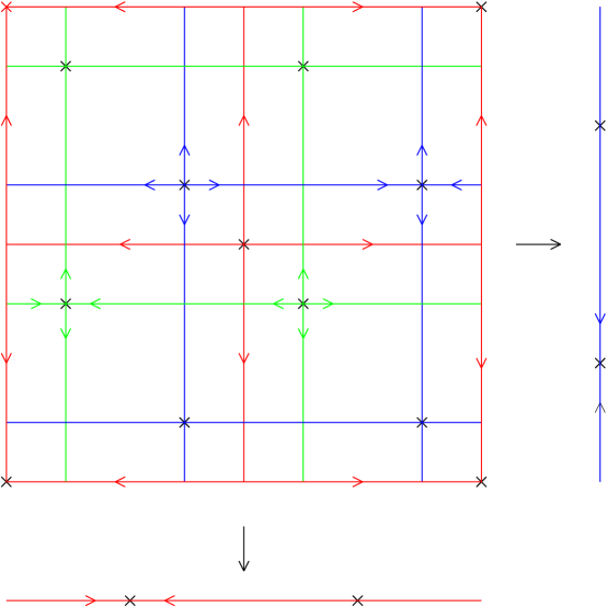
Figure 10. The (negative) flow lines of $(h_{42},g_{42})$, $(h_{20},g_{20})$ on $(\mathbb{R}/\mathbb{Z}\times\mathbb{R}/\mathbb{Z})\cup\mathbb{R}/\mathbb{Z}$ (in red, blue respectively), and $(h_{40},g_{40})$ on $\mathbb{R}/\mathbb{Z}\times\mathbb{R}/\mathbb{Z}$ (in green). The two black arrows indicate projection maps.

Let $\mu_{42}^{j}$ and $\mu_{20}^{j}$ be the Riemannian metrics on $N_{42}^{j}$ and $N_{20}^{j}$ which are of the form $(\phi_{+}^{j})_{*}(g_{S^{1}}\times g_{\mathbb{R}^{2}})$ and $(\phi_{+}^{j})_{*}(g_{S^{1}}\times g_{\mathbb{R}^{2}})$ respectively. Here $\phi_{\pm}^{j}$ are from §5a (and we may assume $N_{42}^{j}$ and $N_{20}^{j}$ are contained in $\phi_{+}^{j}(S^{1}\times D^{2}_{\pi/3})$ and $\phi_{+}^{j}(S^{1}\times D^{2}_{\pi/3})$).

Lemma 7.1.

$((-f_{42}^{j},\mu_{42}^{j});(h_{42}^{j},g_{42}^{j}))\text{ and }((f_{20}^{j},\mu_{20});(h_{20}^{j},g_{42}^{j}))$ are regular Morse-Bott homology data in the sense of §13h. The corresponding ungraded Morse-Bott homology groups with $\mathbb{Z}/2$ coefficients have the following generators and relations.

$$(H_{MB})_{*}((N_{42}^{j},-f_{42}^{j},\mu_{42}^{j}),(h_{42}^{j},g_{42}^{j}),\partial)\text{ is freely generated by }x_{2}^{j},x_{1}^{j}\in\Sigma_{42}^{j};$$

$$(H_{MB})_{*}((N_{20}^{j},f_{20}^{j},\mu_{42}^{j}),(h_{20}^{j},g_{20}^{j}),\partial)\text{ is freely generated by }y_{2}^{j},(y_{1}^{j})^{\prime}\in\Sigma_{20}^{j}.$$

Proof.

We focus on $(-f_{42}^{j},\mu_{42}^{j})$, first addressing regularity. The unstable and stable manifolds of $-f_{42}^{j}$ are both codimension 0 submanifolds of $N_{42}^{j}$, hence they intersect transversely. This shows that $(-f_{42}^{j},\mu_{42}^{j})$ is regular. Next we show that $((-f_{42}^{j},\mu_{42}^{j});(h_{42}^{j},g_{42}^{j}))$ is regular. Let $\mathcal{M}$ denote

$$\{\gamma\in C^{\infty}(\mathbb{R},N_{42}^{j}):\gamma^{\prime}(s)=-\nabla_{\mu_{42}^{j}}(-f_{42}^{j})(\gamma(s)),\gamma(-\infty)\in\Sigma_{42}^{j},\gamma(\infty)\in K_{+}^{j}\},$$

and let $\mathcal{M}^{*}=\mathcal{M}/\mathbb{R}$, $ev_{+}(\gamma)=\gamma(+\infty)$, $ev_{-}(\gamma)=\gamma(-\infty)$. Recall $\mu_{42}^{j}=(\phi_{+}^{j})_{*}(g_{S^{1}}\times g_{\mathbb{R}^{2}})$ on $N_{42}^{j}$, and note that $f_{42}^{j}$ is rotationally symmetric as well. Therefore, for each $(e,f)\in K_{+}^{j}\times K_{-}^{j}$, there is exactly one $\gamma\in\mathcal{M}^{*}$ with $ev_{+}(\gamma)=e$ and $ev_{-}(\gamma)=\varphi_{42}^{j}(e,f)\in\Sigma_{42}^{j}$. This means we can identify $\mathcal{M}^{*}$ with $\mathbb{R}/\mathbb{Z}\times\mathbb{R}/\mathbb{Z}$, where the evaluation maps

$$ev_{+}:\mathcal{M}^{*}\longrightarrow K_{+}^{j},\,ev_{-}:\mathcal{M}^{*}\longrightarrow\Sigma_{42}^{j}\text{ become, respectively,}$$

$$\pi_{+}:\mathbb{R}/\mathbb{Z}\times\mathbb{R}/\mathbb{Z}\longrightarrow\mathbb{R}/\mathbb{Z},\,\pi_{-}:\mathbb{R}/\mathbb{Z}\times\mathbb{R}/\mathbb{Z}\longrightarrow\mathbb{R}/\mathbb{Z}\times\mathbb{R}/\mathbb{Z},$$

where $\pi_{+}$ is projection to the first factor and $\pi_{-}$ is the identity map. Then $((-f_{42}^{j},\mu_{42}^{j});(h_{42}^{j},g_{42}^{j}))$ is regular because $\pi_{-}^{-1}(U(x))\cap\pi_{+}^{-1}(S(a))$ is a transverse intersection for all $x,a\in Crit(h_{42}^{j})$, where $x\in\mathbb{R}/\mathbb{Z}\times\mathbb{R}/\mathbb{Z}\cong\Sigma_{42}^{j}$ and $a\in\mathbb{R}/\mathbb{Z}\cong K_{+}^{j}$. (See figure 10.)

Because $-f_{42}$ has a maximum along $\Sigma_{42}^{j}$, the Morse Bott homology will be isomorphic to $H_{*}(N_{42},\partial N_{42})$. (In general, for a manifold $N$ with boundary, if the Morse-Bott function $f:N\longrightarrow\mathbb{R}$ takes a minimum (resp. maximum) along the boundary, then the Morse-Bott homology of $f$ is isomorphic to $H_{*}(N)$ (resp. $H_{*}(N,\partial N)$).) Since we have already analyzed $\mathcal{M}^{*}$ we may as well verify this explicitly. For $x\in Crit(h_{42}^{j}|\Sigma_{42}^{j})$,

$$\partial x=\Sigma_{a}\#(\pi_{-}^{-1}(U(x))\cap\pi_{+}^{-1}(S(a)))a,$$

where $x$, $a$ are as above and $\#(\pi_{-}^{-1}(U(x))\cap\pi_{+}^{-1}(S(a)))$ is the number of zero dimensional components mod 2. Using this it is easy to see that

$$\partial x_{2}^{j}=0,\,\partial x_{1}^{j}=0,\,\partial(x_{1}^{j})^{\prime}=a_{1}^{j},\,\partial x_{0}^{j}=a_{0}^{j}.$$

For $(H_{MB})_{*}(N_{20}^{j},(f_{20}^{j},\mu_{42}^{j});(h_{20}^{j},g_{20}^{j}),\partial)$ everything is the same except $ev_{+}$ is projection to the second factor. In that case we get

$$\partial y_{2}^{j}=0,\,\partial(y_{1}^{j})^{\prime}=0,\,\partial(y_{1}^{j})=b_{1}^{j},\,\partial y_{0}^{j}=b_{0}^{j}.$$

∎

Now let $(\widetilde{h}_{40}^{j},\widetilde{g}_{40}^{j})$ be any Morse-Smale pair on $\Sigma_{40}^{j}$ such that $\widetilde{h}_{40}^{j}$ has critical points $\tilde{z}_{0}^{\,j},\tilde{z}_{1}^{\,j},(\tilde{z}_{1}^{\,j})^{\prime},\tilde{z}_{2}^{\,j}$ (where the index is given by the subscript) such that the closure of the unstable manifolds

$$\widetilde{\mu}_{j}=\overline{U((\tilde{z}_{1}^{\,j})^{\prime})}\cong S^{1}\text{ and }\widetilde{\lambda}_{j}=\overline{U(\tilde{z}_{1}^{\,j})}\cong S^{1}$$

have linking numbers in $L_{0}\cong S^{3}$ respectively

$$\ell k(\widetilde{\lambda}_{j},K_{j})=0\text{ and }\ell k(\widetilde{\mu}_{j},K_{j})=1.$$

To be concrete, we can take $\widetilde{\lambda}_{j}=\phi_{j}(S^{1}\times\{p\})$ for some $p\in\partial D^{2}$ and $\widetilde{\mu}_{j}=\phi_{j}(\{q\}\times\partial D^{2})$ for some $q\in S^{1}$. Recall the singular homology $H_{*}(N_{40})$ is generated by the cycles $\Sigma_{40}^{j}$, $\widetilde{\lambda}_{j}$, $\widetilde{\mu}_{j}$, $\widetilde{p}_{j}$, $j=1,\ldots,k$, where $\widetilde{p}_{j}\in\Sigma^{j}_{42}$ is any point. The relations are as in §3:

(7.19) $$[\widetilde{\lambda}_{j}]=\Sigma_{i\neq j}\ell k(K_{j},K_{i})[\widetilde{\mu}_{i}];\,\Sigma_{j}[\widetilde{\Sigma}_{40}^{j}]=0;\,[\widetilde{p}_{1}]=\ldots=[\widetilde{p}_{k}].$$

Lemma 7.2.

The Morse-Bott function $f_{40}:N_{40}\longrightarrow\mathbb{R}$ can be chosen (maintaining same form as in §7a) so that, for some metric $\mu_{40}$ on $N_{40}$, the Morse-Bott homology data $((-f_{40},\mu_{40});(\widetilde{h}_{40},\widetilde{g}_{40}))$ is regular in the sense of §13h. Moreover the Morse-Bott homology

$$(H_{MB})_{*}((N_{40},-f_{40},\mu_{40}),(\widetilde{h}_{40},\widetilde{g}_{40}),\partial)$$

is generated by $\tilde{z}_{0}^{\,j},\tilde{z}_{1}^{\,j},(\tilde{z}_{1}^{\,j})^{\prime},\tilde{z}_{2}^{\,j}$, $j=1,\ldots,k$ and the relations are

$$[\tilde{z}_{1}^{\,j}]=\Sigma_{i\neq j}\ell k(K_{j},K_{i})[(\tilde{z}_{1}^{\,i})^{\prime}];\,\,\Sigma_{j}[\tilde{z}_{2}^{\,j}]=0;\,\,[\tilde{z}_{0}^{\,1}]=\ldots=[\tilde{z}_{0}^{\,k}].$$

Proof.

We will describe a suitable handle decomposition of $N_{40}$ and then take $(-f_{40},\mu_{40})$ so that it realizes this handle decomposition. Regularity will easily follow by suitably adjusting the attaching maps by some isotopy, which corresponds to adjusting $\mu_{40}$ by a small isotopy.

Assume for a moment that this has been done. Then, since $-f_{40}$ takes a minimum along $\cup_{j}\Sigma_{40}^{j}\cong\partial N_{40}$, the Morse-Bott homology is isomorphic to the singular homology $H_{*}(N_{40})$ (as in the proof of lemma 7.1), where the generators $\widetilde{\Sigma}_{40}^{j}$, $\widetilde{\lambda}_{j}$, $\widetilde{\mu}_{j}$, $\tilde{p}_{j}$ correspond respectively to $\tilde{z}_{2}^{j}$, $\tilde{z}_{1}^{j}$, $(\tilde{z}_{1}^{j})^{\prime},$ $\tilde{z}_{0}^{j}\in Crit(\tilde{h}_{40}|\widetilde{\Sigma}_{40}^{j}),$ $j=1,\ldots,k$. Thus we have the expected generators and relations from (7.19). (One can also verify this explicitly by inspecting the handle-decomposition we describe below; compare with the end of the proof of lemma 9.2).

We now explain the handle-decomposition of $N_{40}$. Since $-f_{40}$ is Morse-Bott near its minimum value our handle decomposition starts with $\Sigma\times[0,1]$, where $\Sigma=\cup_{j}\widetilde{\Sigma}_{40}^{j}$. Here, the corresponding Morse-Bott function would depend only on the $[0,1]$ factor, and have a single critical point at 1/2, which is a minimum. From now on we attach standard handles in the usual way to $\Sigma\times\{1\}$ because $-f_{40}$ has only isolated critical points away from $\Sigma$.

We do a variation on the standard Heegaard diagram representation of a link complement. Consider the link diagram of $\cup_{j}K_{j}\subset L_{0}$ with over-crossings and under-crossings. We can visualize $\Sigma\times\{1\}$ as the boundary of a tubular neighborhood of the link diagram of $\cup_{j}K_{j}\subset L_{0}=S^{3}$. Each crossing gives rise to two points, one on the bottom of the over-crossing and one on the top of the under-crossing; these two points form an $S^{0}$ and we attach a 1-handle to this $S^{0}$ at each crossing. We denote the result by $X_{1}$.

Now consider the singularized link diagram $D\subset\mathbb{R}^{2}$, where each crossing no longer has over/under information recorded. For each bounded component $U\cong D^{2}$ of $\mathbb{R}^{2}\setminus D$ we attach a 2-handle to $X_{1}$ whose core corresponds to the disk $U$; the attaching circle will run once along a 1-handle each time it encounters a crossing. Let $X_{2}$ denote result of attaching all these 2-handles; it has one $S^{2}$ boundary component for each component of $D$, and the other boundary components are tori, one for each link component $K_{j}$.

To finish, if $X_{2}$ has several components $C_{1},\ldots,C_{l}$ then we attach a 1-handle to each consecutive pair $(C_{1},C_{2}),(C_{2},C_{3}),\ldots,(C_{l-1},C_{l})$, where the attaching regions lie in $\Sigma\times\{1\}$. The result is a new space $X_{2}^{\prime}$ which is connected. The boundary components of $X_{2}^{\prime}$ consist of the the same tori as before, plus one $S^{2}$ component. We attach a 3-handle to this $S^{2}$ and the result is diffeomorphic to $N_{40}$.

Now $(-f_{40},\mu_{40})$ is regular if and only if $U(C)\cap S(C\,^{\prime})$ is transverse for every pair of critical components $C,C\,^{\prime}$. This is in turn means that the attaching sphere of each handle should be transverse to the descending spheres of all handles up to that point. (This does not constrain how the attaching spheres meet the tori.) Also, $((-f_{40},\mu_{40}),(\widetilde{h}_{40},\widetilde{g}_{40}))$ is regular if and only if the attaching sphere of each handle meets $U(\tilde{z})\subset\Sigma\times\{1\}$ transversely in $\Sigma\times\{1\}$ for every $\tilde{z}\in Crit(\widetilde{h}_{40})$. Both of these conditions can be arranged by suitably isotoping the attaching spheres of the handles, and this corresponds to adjusting $\mu_{40}$ by a small isotopy. ∎

7c. Identifying the Floer homology groups with the Morse-Bott homology groups

In this section we identify the Floer homology groups we are interested in with the Morse-Bott homology groups from the last section (in fact the chain complexes are isomorphic). We use the results of §11; there we explain how to replace $V_{4}$ and $V_{0}$ by new exact isotopic versions obtained, roughly speaking, by replacing $df_{40}$, $df_{42}^{j}$, $df_{20}^{j}$ by by $\frac{1}{n}df_{40}$, $\frac{1}{n}df_{42}^{j}$, $\frac{1}{n}df_{20}^{j}$, for some fixed $n\geq 1$ sufficiently large, and patching those back into $V_{4}$ and $V_{0}$ using a cut-off function. Let us assume that this replacement has been made, but we keep the same notation. (Note that the re-scaling $f\leadsto\frac{1}{n}f$ does not affect the arguments in §7b.) Then the main result of §11 is given by the following lemma; it corresponds to Proposition 11.3.

Lemma 7.3.

There exist almost complex structures $J_{40}$, $J_{42}^{j}$, $J_{20}^{j}$ $\in$ $\mathcal{J}([0,1],M,I)$ such that $(J_{42}^{j};h_{42}^{j},g_{42}^{j})$, $(J_{20}^{j};h_{20}^{j},g_{20}^{j})$, $(J_{40};(\widetilde{h}_{40},\widetilde{g}_{40}))$ are each regular as Morse-Bott Floer data (see §13d). Moreover, for every $p$, $q$ $\in$ $Crit(f_{40})$ $=$ $V_{4}\cap V_{0}$, $\mathcal{M}(V_{4},V_{0},J_{40};p,q)$ is in one-one correspondence with

$$\{\gamma\in C^{\infty}(\mathbb{R},N_{40}):\gamma^{\prime}(s)=-\nabla_{\mu_{40}}(-f_{40})(\gamma(s)),\gamma(-\infty)=p,\gamma(\infty)=q\}$$

Similarly, for every $p,q\in Crit(f_{42}^{j})=V_{4}\cap V_{2}^{j}$, $\mathcal{M}(V_{4},V_{2}^{j},J_{42}^{j};p,q)$ is in one-one correspondence with

$$\{\gamma\in C^{\infty}(\mathbb{R},N_{42}^{j}):\gamma^{\prime}(s)=-\nabla_{\mu_{42}^{j}}(-f_{42}^{j})(\gamma(s)),\gamma(-\infty)=p,\gamma(\infty)=q\},\text{ and }$$

for every $p,q\in Crit(f_{20}^{j})=V_{2}^{j}\cap V_{0}$, $\mathcal{M}(V_{2}^{j},V_{0},J_{20}^{j};p,q)$ is in one-one correspondence with

$$\{\gamma\in C^{\infty}(\mathbb{R},N_{20}^{j}):\gamma^{\prime}(s)=-(\nabla_{\mu_{20}^{j}}f_{20}^{j})(\gamma(s)),\gamma(-\infty)=p,\gamma(\infty)=q\}.$$

As an immediate consequence we have the following generators and relations for the Floer homology groups.

Proposition 7.4.

$$HF_{*}((V_{4},V_{2}^{j},J_{42});(h_{42}^{j},g_{42}^{j}))\text{ is freely generated by }x_{2}^{j},x_{1}^{j}\in\Sigma_{42}^{j};$$

$$HF_{*}((V_{2}^{j},V_{0},J_{20});(h_{20}^{j},g_{20}^{j}))\text{ is freely generated by }y_{2}^{j},(y_{1}^{j})^{\prime}\in\Sigma_{20}^{j};$$

and $HF_{*}((V_{4},V_{0},J_{40});(\widetilde{h}_{40},\widetilde{g}_{40}))$ is generated by $\tilde{z}_{0}^{\,j},$ $\tilde{z}_{1}^{\,j},$ $(\tilde{z}_{1}^{\,j})^{\prime},$ $\tilde{z}_{2}^{\,j}\in\Sigma_{40}^{j}$, $j=1,\ldots,k$, with the relations

$$[\tilde{z}_{1}^{\,j}]=\Sigma_{i\neq j}\ell k(K_{j},K_{i})[(\tilde{z}_{1}^{\,i})^{\prime}],\phantom{bb}\Sigma_{j}[\tilde{z}_{2}^{\,j}]=0,\,\,[\tilde{z}_{0}^{1}]=\ldots=[\tilde{z}_{0}^{k}].$$

Proof.

As ungraded complexes with $\mathbb{Z}/2$ coefficients, we have isomorphisms

$$(CF((V_{4},V_{2}^{j},J_{42}),(h_{42}^{j},g_{42}^{j}),\partial)\cong(C_{MB})((N_{42}^{j},-f_{42}^{j},\mu_{42}^{j}),(h_{42}^{j},g_{42}^{j}),\partial).$$

$$(CF((V_{2}^{j},V_{0},J_{20}),(h_{20}^{j},g_{20}^{j}),\partial)\cong(C_{MB})((N_{20}^{j},f_{20}^{j},\mu_{20}^{j}),(h_{20}^{j},g_{20}^{j}),\partial)$$

$$(CF((V_{4},V_{0},J_{40}),(\widetilde{h}_{40},\widetilde{g}_{40}),\partial)\cong(C_{MB})((N_{40},-f_{40},\mu_{40}),(\widetilde{h}_{40},\widetilde{g}_{40}),\partial).$$

All three isomorphisms are given by the identity map (for example from $V_{4}\cap V_{0}$ to $Crit(f_{40})$). The identification of these complexes is immediate from the last lemma, and the definition of these complexes (see §13). Propositions 7.1 and 7.2 then imply the stated generators and relations.∎

Note that the generators and relations in the last proposition match up perfectly with the ones for the flow category (3.15) in §3.

8. The monotonicity lemma; constructing $\widetilde{V}_{4}$, $\widetilde{V}_{2}^{j}$, $\widetilde{V}_{0}$

In this section we carry out the details of the arguments involving the monotonicity lemma (sketched in §4f). In the process we replace $V_{0}$, $V_{2}^{j}$, $V_{4}$ by $\widetilde{V}_{0}$, $\widetilde{V}_{2}^{j}$, $\widetilde{V}_{4}$, which correspond to version IV of the vanishing spheres in §4f.

Let $\Delta$ denote any one of the four triangles bounded by $\Gamma_{4}$, $\Gamma_{2}$ and $\Gamma_{0}$ in figure 9. Let $\widetilde{U}$ be a small connected compact neighborhood of $\Delta$ in $\mathbb{R}/2\pi\mathbb{Z}\times[-r,r]$, where $\widetilde{U}$ is so small that it does not contain the points corresponding to $K_{\pm}^{j}$ (in figure 11, $\widetilde{U}$ is bounded by the largest triangle). Let $\widetilde{B}\subset\widetilde{U}$ be a compact annular subregion which surounds $\Delta$, but does not touch it, and let $\widetilde{B}_{0}\subset\textup{Int\,}\widetilde{B}$ be another smaller compact annular region surounding $\Delta$ (see figure 11, where $\widetilde{B}$ is bounded by the two black triangles, and $\widetilde{B}_{0}$ is bounded by the two brown triangles inside $B$).

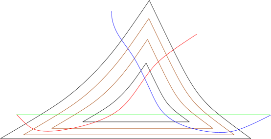
Figure 11. The regions $\widetilde{U},\widetilde{B},\widetilde{B}_{0}$ surounding $\Delta$ in $\mathbb{R}/2\pi\mathbb{Z}\times[-r,r]$.

Now let $T^{j}=\cup_{e,f}\sigma_{ef}^{j}(\Delta)$ (this is the union of all our expected holomorphic triangles) and let $U^{j}\subset D(T^{*}L_{2}^{j})$ be a connected compact neighborhood of $T^{j}$ such that $U^{j}\cap D(T^{*}K_{ef}^{j})=\sigma_{ef}^{j}(\widetilde{U})$ for every $e$, $f$. Similarly, let $B_{0}^{j}\subset B^{j}\subset U^{j}$ be annular regions surounding $T^{j}$ corresponding to $\widetilde{B}_{0}\subset\widetilde{B}\subset\widetilde{U}$ in the sense that $B^{j}\cap D(T^{*}K_{ef}^{j})=\sigma_{ef}^{j}(\widetilde{B})$ and $B^{j}_{0}\cap D(T^{*}K_{ef}^{j})=\sigma_{ef}^{j}(\widetilde{B}_{0})$ for every $e$, $f$. More precisely, we may suppose that $B_{0}^{j}\subset B^{j}\subset U^{j}$ are of the form

$$U^{j}=\{x\in T^{*}L_{2}^{j}:dist(x,T^{j})\leq\eta\},$$

$$B^{j}=\{x\in T^{*}L_{2}^{j}:\lambda\leq dist(x,T^{j})\leq\eta\},\,\,B^{j}_{0}=\{x\in T^{*}L_{2}^{j}:\lambda_{0}\leq dist(x,T^{j})\leq\eta_{0}\},$$

where $0<\lambda<\lambda_{0}<\eta_{0}<\eta$. Then $T^{*}L_{2}^{j}\setminus B^{j}$ has exactly two components, one of which contains $T^{j}$, and similarly for $B_{0}^{j}$.

Let $g$ denote the metric on $\cup_{j}\,D(T^{*}L_{2}^{j})$ determined by $\omega|(\cup_{j}\,D(T^{*}L_{2}^{j}))$ and $J_{\mathbb{C}}$. Fix $\mu>0$ such that for every $y\in B_{0}^{j}$ we have

(8.20) $$D_{\mu}^{\,g}(y)=\{x\in D(T^{*}L_{2}^{j}):dist_{g}(x,y)\leq\mu\}\subset B^{j}.$$

Also assume that $\mu$ is small enough that

$$exp_{y}^{\,g}:D_{\mu}(T_{y}(T^{*}L_{2}^{j}),g)\longrightarrow D_{\mu}^{g}(y)$$

is a diffeomorphism for any $y\in B_{0}^{j}$. We have the following relative form of the monotonicity lemma (see [FSS08] lemma 12). (The essential ingredient is an isoperimetric inequality, with respect to the metric $g$, applied inside small balls $D_{\mu}^{g}(y)$.)

Lemma 8.1.

Fix $j=1,\ldots,k$. Suppose $L$ is a (not necessarily connected) Lagrangian submanifold of $B^{j}$ with $\partial L\subset\partial B^{j}$. Set

$$d=(1/2)min\{dist(C,C^{\prime}):C,C^{\prime}\text{ are distinct components of L}\}.$$

There are constants $0<\gamma,0<\rho<min(\mu,d)$, depending on $L$, $J_{\mathbb{C}}|(\cup_{j}B^{j})$, and $\omega|(\cup_{j}B^{j})$ such that the following holds. Let $\Sigma$ be a compact Riemann surface with (nonempty) boundary with corners, and let $u:\Sigma\longrightarrow B^{j}$ be a nonconstant $J_{\mathbb{C}}-$holomorphic curve such that there is some $y\in B_{0}^{j}\cap u(\Sigma)$, and $u(\partial\Sigma)\subset\partial D_{s}^{g}(y)\cup L$ for some $0<s\leq\rho$. Then

$$\int_{\Sigma}u^{*}\omega\geq\gamma s^{2}.\,\square$$

Remark 8.2.

It doesn’t matter that $B^{j}$ has boundary because the proof of this type of lemma takes place on small balls of radius less than $\mu$ centered at points $y\in B_{0}$, which are contained in $\textup{Int\,}(B)$. Also, the version of this lemma in [FSS08] assumes that $L$ is connected. Because $\rho$ is less than half the distance between any pair of components of $L$, we can apply that version to each component successively, shrinking $\rho$ each time, to deduce the version above.

We will apply the above lemma to $L=L^{j}$, where

$$L^{j}=(V_{4}\cap B^{j})\cup(V_{0}\cap B^{j})\cup(V_{2}^{j}\cap B^{j})$$

From figure 11 we see that $L^{j}$ is a smooth Lagrangian (not connected) submanifold of $B^{j}$ with $\partial L_{j}\subset\partial B_{j}$.

Fix an $I\in\mathcal{J}(M)$ which makes $\partial M$ $I-$convex. Equip $T^{*}L_{2}^{j}=T^{*}S^{3}$ the complex structure $J_{\mathbb{C}}$ inherited from the symplectic identification $T^{*}S^{3}\cong\{z\in\mathbb{C}^{4}:\Sigma_{i}z_{i}^{2}=1\}$ (see page 12). Fix any $J\in\mathcal{J}(V,M,I)$ which satisfies

(8.21) $$J_{\zeta}|U^{j}=J_{\mathbb{C}}|U^{j}\text{ for all }j\text{ and for all }\zeta\in V.$$

Lemma 8.3.

There is a constant $\epsilon>0$ depending on $J_{\mathbb{C}}|(\cup_{j}B^{j})$, $\cup_{j}L^{j}\subset\cup_{j}B^{j}$, and $\omega|(\cup_{j}B^{j})$ such that the following holds. Let $J\in\mathcal{J}(V,M,I)$ satisfy (8.21); then for any $w\in\mathcal{M}(M,V_{4},V_{2}^{j},V_{0},J)$, if $w(p)\in B_{0}^{j}$ for some $p$ then $\int_{V}w^{*}\omega\geq\epsilon.$

Proof.

Set $y=w(p)\in B_{0}^{j}$. We invoke lemma 8.1 for $L^{j}$ as defined above. Let $\rho>0$ and $\gamma>0$ be the resulting constants. Now take $s>0$ such that $\rho/2<s<\rho$ and such that $w$ is transverse to $\partial D_{s}^{\,g}(y)$. Set $\Sigma=w^{-1}(D_{s}^{\,g}(y))$. Then $w(\partial\Sigma)\subset\partial D_{s}^{\,g}(y)\cup L^{j}$. We have $\partial\Sigma\neq\emptyset$ and $w|\Sigma$ nonconstant because of the boundary conditions for $w$ and because $D_{s}^{\,g}(y)\subset\textup{Int\,}(B^{j})$. Lemma 8.1 applied to $u=w|\Sigma$ says that

$$\int_{V}w^{*}\omega\geq\int_{\Sigma}u^{*}\omega\geq\gamma s^{2}\geq\gamma\rho^{2}/4,$$

so we can take $\epsilon=\gamma\rho^{2}/4.$ ∎

We now consider new Lagrangians $\widetilde{V}_{4}$, $\widetilde{V}_{2}^{j}$, $\widetilde{V}_{0}$, obtained by applying exact isotopies to $V_{4}$, $V_{2}^{j}$, $V_{0}$. These isotopies arise by adjusting $\Gamma_{4}$, $\Gamma_{2}$, $\Gamma_{0}$ in $\mathbb{R}/2\pi\mathbb{Z}\times[-r,r]$ by exact isotopies as in figure 12.

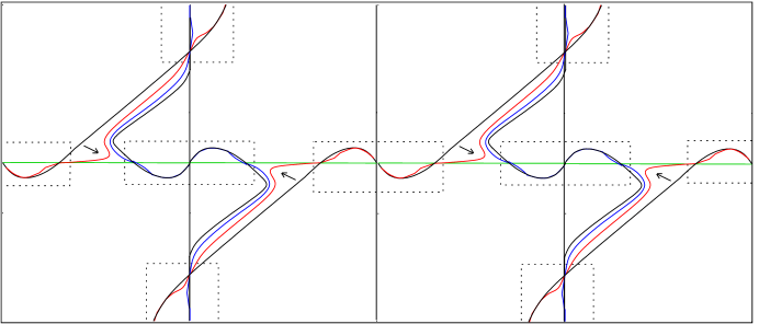
Figure 12. $\widetilde{\Gamma}_{4}$ (red), $\widetilde{\Gamma}_{2}$ (green), $\widetilde{\Gamma}_{0}$ (blue) in $\mathbb{R}/2\pi\mathbb{Z}\times[-r,r]$.

The new versions $\widetilde{\Gamma}_{4}$, $\widetilde{\Gamma}_{2}$, $\widetilde{\Gamma}_{0}$ are chosen so that the four triangles bounded by $\widetilde{\Gamma}_{4}$, $\widetilde{\Gamma}_{2}$, $\widetilde{\Gamma}_{0}$ each have area less that $\epsilon$ (from lemma 8.3). In addition, the boundary arcs of each triangle are chosen to be real analytic (we will need this to construct $w_{ef}^{j}$ as in Proposition 8.6). In order for this to happen, the new $\widetilde{\Gamma}$’s must interpolate back to the old $\Gamma$’s away from the triangles; that is why there are small humps between $\Gamma_{i}$ and $\widetilde{\Gamma}_{i}$ at each vertex. However, we also insist that $\widetilde{\Gamma}_{i}\cap\widetilde{B}=\Gamma_{i}\cap\widetilde{B}$ (this is ensured if the small humps at each vertex are small enough). The last condition implies that $\widetilde{V}_{4}\cap B=V_{4}\cap B$, $\widetilde{V}_{2}^{j}\cap B=V_{2}^{j}\cap B$, and $\widetilde{V}_{0}\cap B=V_{0}\cap B$. Thus, for any $w\in\mathcal{M}(M,\widetilde{V}_{4},\widetilde{V}_{2}^{j},\widetilde{V}_{0},J)$,

(8.22) $$\text{ if }w(p)\in B_{0}^{j}\text{ for some }p,\text{ then }\int_{V}w^{*}\omega\geq\epsilon,$$

where $\epsilon$ is the same one from lemma 8.3. (Note the proof of lemma 8.3 takes place entirely in $B$, so it will not feel the difference between $\widetilde{V}_{4}$, $\widetilde{V}_{2}^{j}$, $\widetilde{V}_{0}$, and $V_{4}$, $V_{2}^{j}$, $V_{0}$.)

We keep the same notation $\Delta\subset\mathbb{R}/2\pi\mathbb{Z}\times[-r,r]$ for any one of the four triangles bounded by $\widetilde{\Gamma}_{4}$, $\widetilde{\Gamma}_{2}$, $\widetilde{\Gamma}_{0}$. Note that the new functions $f_{40}$, $f_{42}^{j}$, $f_{20}^{j}$, corresponding to $\widetilde{V}_{4}$, $\widetilde{V}_{2}^{j}$, $\widetilde{V}_{0}$ have the same basic form, so we keep the same notation there as well.

Lemma 8.4.

Let $J\in\mathcal{J}(V,M,I)$ satisfy (8.21), and let $w\in\mathcal{M}(\widetilde{V}_{4},\widetilde{V}_{2}^{j},\widetilde{V}_{0},J;M)$ for some $j=1,\ldots,k$. Then the symplectic area of $w$ is less than or equal to the Euclidean area of the triangle $\Delta\subset\mathbb{R}/2\pi\mathbb{Z}\times\mathbb{R}$, hence it is less than $\epsilon$ (from lemma 8.3).

Proof.

Let $w:V\longrightarrow M$ be any smooth map, which extends continuously to $D^{2}$, and which satisfies $w(I_{0})\subset\widetilde{V}_{0}$, $w(I_{1})\subset\widetilde{V}_{2}^{j}$, $w(I_{2})\subset\widetilde{V}_{4}$ (for example, any $w\in\mathcal{M}(\widetilde{V}_{4},\widetilde{V}_{2}^{j},\widetilde{V}_{0},J;M)$). Then

$$p_{40}=\lim_{\zeta\rightarrow\zeta_{0}}w(\zeta)\in\Sigma_{40}^{j}\cup\{\text{isolated critical points of }f_{40}\},$$

$$p_{42}=\lim_{\zeta\rightarrow\zeta_{1}}w(\zeta)\in K_{+}^{j}\cup\Sigma_{42}^{j},\text{ and }p_{20}=\lim_{\zeta\rightarrow\zeta_{2}}w(\zeta)\in K_{+}^{j}\cup\Sigma_{20}^{j}.$$

Take functions $k_{0},k_{2},k_{4}$ defined on $\widetilde{V}_{0},(\cup_{j}\widetilde{V}_{2}^{j}),\widetilde{V}_{4}$ respectively, such that $\theta|\widetilde{V}_{2}^{j}=dk_{2}$, $\theta|\widetilde{V}_{0}=dk_{0}$, $\theta|\widetilde{V}_{4}=dk_{4}$. Up to adding constants we have,

$$k_{4}|(\widetilde{V}_{4}\cap D(T^{*}N_{42}))=f_{42},\,k_{4}|(\widetilde{V}_{4}\cap D(T^{*}N_{40}))=f_{40},\,k_{0}|(\widetilde{V}_{0}\cap D(T^{*}N_{20}))=f_{20},$$

Then, by Stoke’s theorem,

(8.23) $$\int_{V}w^{*}\omega=k_{4}(p_{40})-k_{4}(p_{42})+k_{2}(p_{42})-k_{2}(p_{20})+k_{0}(p_{20})-k_{0}(p_{40}).$$

Consider the case when all three vertices lie on the tori, $p_{kl}\in\Sigma_{kl}^{j}$. Then $\int_{V}w^{*}\omega=area(\Delta)$ because the above formula shows the symplectic area will not change if we assume $w$ to be of the form $\sigma_{ef}^{j}\circ\varphi$, where $\varphi:V\longrightarrow\mathbb{R}/2\pi\mathbb{Z}\times[-r,r]$ is a smooth map parametrizing $\Delta$, and then, using the coordinates $(u,v)$ on $T^{*}L_{2}^{j}$,

$$\int_{V}(\sigma_{ef}^{j}\circ\varphi)^{*}\omega=\ \int_{V}(\sigma_{ef}^{j}\circ\varphi)^{*}(\Sigma_{k}\,dv_{k}\wedge du_{k})=\int_{V}\varphi^{*}(d\lambda\wedge d\theta).$$

(Note: $\varphi$ should be orientation reversing; compare with the proof of Proposition 12.4.) Now consider the case $p_{40}\in\{\text{isolated critical points of }f_{40}\}$, $p_{42}\in\Sigma_{42}^{j}$, and $p_{20}\in\Sigma_{20}^{j}$. Let $\widetilde{w}:V\longrightarrow M$ be second map satisfying the same conditions, except this time with $q=\lim_{\zeta\rightarrow\zeta_{0}}\widetilde{w}(\zeta)\in\Sigma_{40}^{j}$. Then $\int_{V}\widetilde{w}^{*}\omega=area(\Delta)$, but also $\int_{V}\widetilde{w}^{*}\omega$ is given by the same formula (8.23), but with $p_{40}$ replaced by $q$. Therefore,

$$\int_{V}w^{*}\omega=area(\Delta)-k_{4}(q)+k_{4}(p_{40})-k_{0}(q)+k_{0}(p_{40}).$$

Since $k_{4}=f_{40}$ in $D(T^{*}N_{40})$, and $f_{40}$ takes a maximum at $\Sigma_{40}^{j}$ (and we may assume the value of $f_{40}$ at all isolated critical points is much smaller) it follows that $-k_{4}(q)+k_{4}(p_{40})<0$. Similarly, by inspecting the shape of $\widetilde{\Gamma}_{0}$ near the vertex of $\Delta$ corresponding to $\Gamma_{4}\cap\Gamma_{0}$ (see figure 12), we see that $k_{0}$ has a maximum along $\Sigma_{40}^{j}$, and decreases to some constant value in the region where $p_{40}$ lies. Therefore $-k_{0}(q)+k_{0}(p_{40})<0$ as well. We conclude $\int_{V}w^{*}\omega<area(\Delta)$ (if it is negative, it means that no such holomorphic $w$ could exist). The other cases, $p_{42}\in K_{+}^{j}$, and/or $p_{20}\in K_{-}^{j}$, are handled similarly; one uses the fact that $f_{42}$ has a maximum at $\Sigma_{40}^{j}$, and $f_{20}$ has a minimum at $\Sigma_{20}^{j}$. ∎

Now (8.22) and lemma 8.4 immediately imply:

Proposition 8.5.

Any $w\in\mathcal{M}(\widetilde{V}_{4},\widetilde{V}_{2}^{j},\widetilde{V}_{0},J;M)$ must be contained in the interior of $U^{j}\subset T^{*}L_{2}^{j}$. $\square$

Recall that $J|U^{j}=J_{\mathbb{C}}|U^{j}$. In §12 we classify all $J_{\mathbb{C}}-$holomorphic triangles in $T^{*}L_{2}^{j}$, as summarized in Proposition 8.6 below. Let $\delta_{42},\delta_{20},\delta_{40}$ denote the vertices of $\Delta$, where $\delta_{ij}\in\Gamma_{i}\cap\Gamma_{j}$, $i,j=0,2,4$, and set $\Delta^{*}=\Delta\setminus\{\delta_{42},\delta_{20},\delta_{40}\}.$ Note that $\sigma_{ef}^{j}(\delta_{40})\in\Sigma_{40}^{j}$, $\sigma_{ef}^{j}(\delta_{42})\in\Sigma_{42}^{j}$, and $\sigma_{ef}^{j}(\delta_{20})\in\Sigma_{20}^{j}$. Below $W_{4}^{j}=\widetilde{V}_{4}\cap D(T^{*}L_{2}^{j})$, $W_{2}^{j}=\widetilde{V}_{2}^{j}\cap D(T^{*}L_{2}^{j})$, $W_{0}^{j}=\widetilde{V}_{0}\cap D(T^{*}L_{2}^{j})$.

Proposition 8.6.

(1) (Existence) For each $e\in K_{+}^{j}$, $f\in K_{-}^{j}$ there exists $w_{ef}^{j}\in\mathcal{M}(W_{4}^{j},W_{2}^{j},W_{0}^{j},J_{\mathbb{C}};D(T^{*}L_{2}^{j}))$ which satisfies $w_{ef}^{j}(V)=\sigma_{ef}^{j}(\Delta^{*})\subset D(T^{*}K_{ef}^{j}),$ and

$$\lim_{\zeta\rightarrow\zeta_{0}}w(\zeta)=\sigma_{ef}^{j}(\delta_{40}),\,\,\lim_{\zeta\rightarrow\zeta_{1}}w(\zeta)=\sigma_{ef}^{j}(\delta_{20}),\,\,\lim_{\zeta\rightarrow\zeta_{2}}w(\zeta)=\sigma_{ef}^{j}(\delta_{42}).$$

(2) (Uniqueness) Every $w\in\mathcal{M}(W_{4}^{j},W_{2}^{j},W_{0}^{j},J_{\mathbb{C}};D(T^{*}S^{3}))$ is equal to $w_{ef}^{j}$ for some $e,f$. (3) (Regularity) $J_{\mathbb{C}}$ is regular.

Remark 8.7.

The above result implies in particular that no

$$w\in\mathcal{M}(W_{4}^{j},W_{2}^{j},W_{0}^{j},J_{\mathbb{C}};D(T^{*}L_{2}^{j}))$$

touches the boundary of $D(T^{*}L_{2}^{j})$, or the boundary of $W_{4}^{j}$, $W_{0}^{j}$. This is proved by composing a given $w$ with a certain holomorphic map $P:T^{*}L_{2}^{j}\longrightarrow\mathbb{C}$ and applying the maximum principle.

From Propositions 8.6 and 8.5 we conclude:

Proposition 8.8.

We have an equality of moduli spaces

$$\mathcal{M}(J,\widetilde{V}_{4},\widetilde{V}_{2}^{j},\widetilde{V}_{0};M)=\mathcal{M}(W_{4}^{j},W_{2}^{j},W_{0}^{j},J_{\mathbb{C}};D(T^{*}L_{2}^{j}))$$

Moreover, $J$ is a regular almost complex structure.

9. Computing the continuation map

In this section we give a precise treatment of the argument summarized in §4g. The main point is to show $HF(\widetilde{V}_{4},\widetilde{V}_{0})$, $HF(\widetilde{V}_{4},\widetilde{V}_{2}^{j})$, and $HF(\widetilde{V}_{2}^{j},\widetilde{V}_{0})$, inherit the same generators and relations from Proposition 7.4; recall these match up perfectly with the ones for the flow category (3.15) in §3.

For $HF(\widetilde{V}_{4},\widetilde{V}_{0})$, $HF(\widetilde{V}_{4},\widetilde{V}_{2}^{j})$, $HF(\widetilde{V}_{2}^{j},\widetilde{V}_{0})$, we take the same Morse-Smale data as in §7b: $(h_{42}^{j},g_{42}^{j})$, $(h_{20}^{j},g_{20}^{j})$, and $(\widetilde{h}_{40}^{j},\widetilde{g}_{40}^{j})$ on $\Sigma_{42}^{j}\cup K_{+}^{j}$, $\Sigma_{20}^{j}\cup K_{-}^{j}$, and $\Sigma_{40}^{j}$, respectively. For the almost complex structures let

$$\widetilde{J}_{42}^{j},\widetilde{J}_{20}^{j},\widetilde{J}_{40}\in\mathcal{J}([0,1],M,I),j=1,\ldots,k.$$

be such that

(9.24) $$(\widetilde{J}_{42}^{j})_{t}|U,(\widetilde{J}_{20}^{j})_{t}|U,(\widetilde{J}_{40})_{t}|U=J_{\mathbb{C}},t\in[0,1],$$

and assume that the following Morse-Bott Floer data are regular:

$$(\widetilde{J}_{42}^{j},(h_{42}^{j},g_{42})),(\widetilde{J}_{20}^{j},(h_{20}^{j},g_{20}))(\widetilde{J}_{40},(h_{40}^{j},g_{40})).$$

To see that regularity can be achieved under the above constraints, we follow a basic principle outlined in [MS94, p. 35]: If every nonconstant $J-$holomorphic curve meets some neighborhood $\Omega$, then to make $J$ regular it suffices to perturb $J$ on $\Omega$ only. In our situation, we fix a neighborhood $\Omega\subset(M\setminus\cup_{j}U^{j})$ containing $\cup_{j}(K_{+}^{j}\cup K_{-}^{j})$ as well as all isolated critical point of $f_{40}$ (this is possible by construction of the $U^{j}$: see figure 11). Now note that every nonconstant finite area holomorphic strip will meet $\Omega$, and, since $\Omega\subset(M\setminus\cup_{j}U^{j})$, we can pick $\widetilde{J}_{40}$ $\widetilde{J}_{42}^{j}$, and $\widetilde{J}_{40}$ with complete freedom on $\Omega$.

In fact, we can obviously pick all $\widetilde{J}_{20}^{j}$ to be equal and similarly for $\widetilde{J}_{42}^{j}$; so, for convenience of notation can drop the $j$’s and denote these by $\widetilde{J}_{20}$, $\widetilde{J}_{42}$. Now pick $J\in\mathcal{J}(V,M,I)$ compatible with $\widetilde{J}_{40}$ $\widetilde{J}_{42}$, and $\widetilde{J}_{20}$ in the sense of (13.42), that is, for all $(s,t)\in[0,\infty)\times[0,1]$,

$$J_{\epsilon_{0}(s,t)}=(\widetilde{J}_{40})_{t},\,J_{\epsilon_{1}(-s,t)}=(\widetilde{J}_{42})_{t},\,J_{\epsilon_{2}(-s,t)}=(\widetilde{J}_{20})_{t},\text{ and }J_{\zeta}|U=J_{\mathbb{C}},\,\zeta\in V.$$

The first three conditions are compatible with last one, since each $\widetilde{J}_{t}$ satisfies (9.24). Since $J$ satisfies (8.21), the whole discussion in §8 applies to $J$; in particular we have Proposition 8.8, and $J$ is regular.

We now pick some smooth functions $G,H:M\longrightarrow\mathbb{R}$ such that their Hamiltonian flows satisfy $\phi_{1}^{H}(V_{4})=\widetilde{V}_{4}$ and $\phi_{1}^{G}(V_{0})=\widetilde{V}_{0}$. These will be determined by $H_{0},G_{0}:\mathbb{R}/2\pi\mathbb{Z}\times[-r,r]\longrightarrow\mathbb{R}$ which satisfy $\phi_{1}^{H_{0}}(\Gamma_{4})=\widetilde{\Gamma}_{4}$ and $\phi_{1}^{G_{0}}(\Gamma_{0})=\widetilde{\Gamma}_{0}$. Consider a Weinstein tubular neighborhood of $\Gamma_{0}$, say $D(T^{*}\Gamma_{0})\subset\mathbb{R}/2\pi\mathbb{Z}\times[-r,r]$, which contains $\widetilde{\Gamma}_{0}$ in its interior. Inside $D(T^{*}\Gamma_{0})$, we view $\widetilde{\Gamma}_{0}$ as the graph of an exact 1-form $g^{\prime}(x)dx$, where $x\in[0,1]\cong\Gamma_{0}$ is some coordinate. Similarly, we view $\widetilde{\Gamma}_{4}$ as the graph of $h^{\prime}(x)dx$ over $\widetilde{\Gamma}_{4}$. Then the graphs of $g^{\prime}$, $h^{\prime}$, $g$, and $h$ are as shown in figure 13. (The graphs of $g^{\prime}$ and $h^{\prime}$ are found by inspecting figure 12 and copying out $\widetilde{\Gamma}_{0}$ and $\widetilde{\Gamma}_{4}$, viewed as graphs of functions over $\Gamma_{0}$ and $\Gamma_{4}$.)

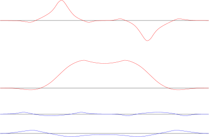
Figure 13. From top to bottom: the graphs of $h^{\prime}$ and $h$ (red), and the graphs of $g^{\prime}$ and $g$ (blue).

Note that in figure 13 (compare with figure 12) the two minima of $h$ correspond to points in $\Sigma_{40}^{j}$, and the two maxima correspond to points in $\Sigma_{42}^{j}$. Similarly, the two maxima of $g$ correspond to points in $\Sigma_{40}^{j}$, and the two minima correspond to points in $\Sigma_{20}^{j}$.

Let $(x,y)$ denote the usual coordinates on $D(T^{*}[0,1])$, then we define $G_{0}$, $H_{0}$ to be zero outside of $D(T^{*}\Gamma_{0})\cong D(T^{*}[0,1])$ and $D(T^{*}\Gamma_{4})\cong D(T^{*}[0,1])$, and on those regions we set $H_{0}(x,y)=-\psi(|y|)h(x)$, $G_{0}(x,y)=-\psi(|y|)g(x),$ where $\psi$ is some suitable cut-off function which makes $G_{0}$, $H_{0}$ equal to zero near the horizontal boundary of $D(T^{*}[0,1])$. (Note that we have taken $g$ and $h$ to be zero near the boundary of $[0,1]$ also.) We need the $-$ signs in order to have $\phi_{1}^{H_{0}}(\Gamma_{4})=\widetilde{\Gamma}_{4}$ and $\phi_{1}^{G_{0}}(\Gamma_{0})=\widetilde{\Gamma}_{0}$. This is because of our conventions (see §13a) and because the symplectic form on $\mathbb{R}/2\pi\mathbb{Z}\times[-r,r]$ is $d\lambda\wedge d\theta$, where $(\theta,\lambda)\in\mathbb{R}/2\pi\mathbb{Z}\times[-r,r]$ (see Proposition 12.4 to see why). Now let us take coordinates on $D(T^{*}L_{2}^{j})=D_{r}^{g_{2}}(T^{*}S^{3})$ given by $(u,v)\in\mathbb{R}^{4}\times\mathbb{R}^{4}$, $|u|=1$, $u\cdot v=0$, where

$$u=(\cos\theta e,\sin\theta f),\phantom{bbb}v=\lambda_{1}(-\sin\theta e,\cos\theta f)+\lambda_{2}(J_{0}e)+\lambda_{3}(J_{0}f)$$

where $\lambda_{1},\lambda_{2},\lambda_{3}\in\mathbb{R}$, $e\in K_{+}^{j}$, $f\in K_{-}^{j}$, $\theta\in\mathbb{R}/2\pi\mathbb{Z}$, $J_{0}e$ $=$ $J_{0}(e_{1},e_{2},0,0)$ $=$ $(e_{2},-e_{1},0,0)$, similarly for $J_{0}f$, and $(g_{2})_{u}(v,v)\leq r^{2}$. Then define

$$G,H:D(T^{*}L_{2}^{j})\longrightarrow\mathbb{R},\phantom{bbb}H(u,v)=H_{0}(\theta,\lambda_{1}),\phantom{bbb}G(u,v)=G_{0}(\theta,\lambda_{1}).$$

Since $G$ and $H$ are both zero near $\partial D(T^{*}L_{2}^{j})$, we can extend them by zero to the rest of $M$, and we denote these also by $G$, $H$. Then we have $\phi_{1}^{H}(V_{4})=\widetilde{V}_{4}$ and $\phi_{1}^{G}(V_{0})=\widetilde{V}_{0}.$ Because we have defined $G$ and $H$ in a symmetrical way explicitly in terms of $g$ and $h$, we can see from figure 13 that $H$ has an absolute minimum at $\Sigma_{40}^{j}$ and an absolute maximum at $\Sigma_{42}^{j}$. Similarly, $G$ has an absolute maximum at $\Sigma_{40}^{j}$ and an absolute minimum at $\Sigma_{20}^{j}$.

Recall there is an elementary isomorphism of moduli spaces

$$\mathcal{M}(L_{0},L_{1},\{H_{t}\},\{J_{t}\})\longrightarrow\mathcal{M}(L_{0},(\phi_{1}^{H})^{-1}(L_{1}),0,\{(\phi_{t}^{H})^{*}J_{t}\})$$

given by $u\mapsto\widetilde{u}$, where $\widetilde{u}(s,t)=(\phi^{H}_{t})^{-1}(u(s,t))$. This isomorphism also has a version at the linearized level which carries regular data into regular data. From this we obtain $HF(L_{0},(\phi_{1}^{H})^{-1}(L_{1}),0,\{J_{t}\})\cong HF(L_{0},L_{1},\{H_{t}\},\{(\phi_{t}^{H})_{*}J_{t}\})$. We apply this (as well as a simpler isomorphism where one pushes everything forward by a symplectomorphism) and obtain

$$HF(\widetilde{V}_{4},\widetilde{V}_{0},0,\{(\widetilde{J}_{40})_{t}\})=HF(\phi_{1}^{H}(V_{4}),\phi_{1}^{G}(V_{0}),0,\{(\widetilde{J}_{40})_{t}\})$$

$$\cong HF(V_{4},((\phi_{1}^{H})^{-1}\circ\phi_{1}^{G})(V_{0}),0,\{(\phi_{1}^{H})^{-1}_{*}(\widetilde{J}_{40})_{t}\})$$

$$=HF(V_{4},(\phi_{1}^{(G-H)\circ\phi_{t}^{G}})^{-1}(V_{0}),0,\{(\phi_{1}^{H})^{-1}_{*}(\widetilde{J}_{40})_{t}\})$$

$$\cong HF(V_{4},V_{0},\{(G-H)\circ\phi_{t}^{G}\},\{(\phi_{1}^{(G-H)\circ\phi_{t}^{G}})_{*}(\phi_{1}^{H})^{-1}_{*}(\widetilde{J}_{40})_{t}\}).$$

Above we have used $(\phi_{t}^{F})^{-1}=\phi_{t}^{\{-F\circ\phi_{t}^{F}\}}$ and $\phi_{t}^{\{G_{t}\}}\circ\phi_{t}^{\{H_{t}\}}=\phi_{t}^{\{G_{t}+H_{t}\circ(\phi^{G}_{t})^{-1}\}}$. Similarly, we have

$$HF(\widetilde{V}_{4},\widetilde{V}_{2}^{j},0,\{(\widetilde{J}_{42})_{t}\})=HF(\phi_{1}^{H}(V_{4}),V_{2}^{j},0,\{(\widetilde{J}_{42})_{t}\})$$

$$\cong HF(V_{4},V_{2}^{j},H,\{(\phi_{t}^{H})_{*}(\phi_{1}^{H})^{-1}_{*}(\widetilde{J}_{42})_{t}\}),\text{ and }$$

$$HF(\widetilde{V}_{2}^{j},\widetilde{V}_{0},0,\{(\widetilde{J}_{20})_{t}\})=HF(V_{2}^{j},(\phi_{1}^{-G\circ\phi_{t}^{G}})^{-1}(V_{0}),0,\{(\widetilde{J}_{20})_{t}\})$$

$$\cong HF(V_{2}^{j},V_{0},\{-G\circ\phi_{t}^{G}\},\{(\phi_{t}^{-G\circ\phi_{t}^{G}})_{*}(\widetilde{J}_{20})_{t}\}).$$

As we mentioned above, all these new Floer data $(H,J)$ for $V_{4}$, $V_{2}^{j}$, $V_{0}$ are regular. Now set $(H_{40}^{\alpha})_{t}=0$, $(H_{42}^{\alpha})_{t}=H$, $(H_{20}^{\alpha})_{t}=-G\circ\phi_{t}^{G}$, $H_{40}^{\beta}=(G-H)\circ\phi_{t}^{G}$, $H_{42}^{\beta}=0$, $H_{20}^{\beta}=0$, for $t\in[0,1]$. Note that $(H_{40}^{\alpha})_{t}$ has an absolute maximum at $\Sigma_{40}^{j}$ for all $t\in[0,1]$, and $(H_{42}^{\alpha})_{t}$, $(H_{20}^{\alpha})_{t}$ each have an absolute minimum respectively at $\Sigma_{42}^{j}$, $\Sigma_{20}^{j}$. (For example, to see this for $(H_{40}^{\alpha})_{t}$, note that $G$ and $-H$ both have a maximum at $\Sigma_{40}^{j}$, and $\phi_{t}^{G}$ is a diffeomorphism which fixes $\Sigma_{40}^{j}$ point-wise for all $t$.) Add constants to each of $(H_{40}^{\alpha})_{t}$, $(H_{42}^{\alpha})_{t}$ and $(H_{20}^{\alpha})_{t}$ so that these maxima and minima are all equal to zero. We take homotopies of time dependent Hamiltonians,

$$(H_{40}^{\alpha\beta})_{s,t},(H_{42}^{\alpha\beta})_{s,t},(H_{20}^{\alpha\beta})_{s,t}:M\longrightarrow\mathbb{R},s\in\mathbb{R},t\in[0,1],\text{ with}$$

$$(H_{40}^{\alpha\beta})_{s,t}=\varphi(s)(H_{40}^{\alpha})_{t},\,(H_{42}^{\alpha\beta})_{s,t}=\varphi(s)(H_{42}^{\alpha})_{t},\,(H_{20}^{\alpha\beta})_{s,t}=\varphi(s)(H_{20}^{\alpha})_{t},$$

where $\varphi:\mathbb{R}\longrightarrow\mathbb{R}$ is some monotone cut-off function with $\varphi(s)=1$ for $s\leq-1$ and $\varphi(s)=0$ for $s\geq 1$. Because $\partial_{s}(H_{40}^{\alpha\beta})_{s,t}(p)\leq 0$ for all $p\in M$, $s\in\mathbb{R}$, $t\in[0,1]$, we say that $(H_{40}^{\alpha\beta})_{s,t}$ is a monotone homotopy (see [CFH95, FH93, CR06]), and similarly for $(H_{42}^{\alpha\beta})_{s,t}$, $(H_{20}^{\alpha\beta})_{s,t}$. This condition will be important in what follows. Set

$$(J_{40})_{t}^{\alpha}=(J_{40})_{t},\phantom{bb}(J_{40}^{\beta})_{t}=(\phi_{1}^{(G-H)\circ\phi_{t}^{G}})_{*}(\phi_{1}^{H})^{-1}_{*}(\widetilde{J}_{40})_{t},$$

$$(J_{42}^{\alpha})_{t}=(\phi_{t}^{H})_{*}(\phi_{1}^{H})^{-1}_{*}(\widetilde{J}_{42})_{t},\phantom{bb}(J_{42})_{t}^{\beta}=(J_{42})_{t},\text{ and }$$

$$(J_{20}^{\alpha})_{t}=(\phi_{t}^{-G\circ\phi_{t}^{G}})_{*}(\widetilde{J}_{20})_{t},\phantom{bb}(J_{20})_{t}^{\beta}=(J_{20})_{t}.$$

Pick homotopies of almost complex structures $(J_{40}^{\alpha\beta})_{s,t}$, $(J_{42}^{\alpha\beta})_{s,t}$, $(J_{20}^{\alpha\beta})_{s,t}$ respectively equal to $(J_{40}^{\alpha})_{t}$, $(J_{42}^{\alpha})_{t}$, $(J_{20}^{\alpha})_{t}$ for $s\leq-1$ and equal to $(J_{40}^{\beta})_{t}$, $(J_{42}^{\beta})_{t}$, $(J_{20})_{t}^{\beta}$ for $s\geq 1$. We will consider the continuation map

$$\phi_{40}:HF(V_{4},V_{0},H^{\alpha}_{40},J^{\alpha}_{40})\longrightarrow HF(V_{4},V_{0},H^{\beta}_{40},J^{\beta}_{40}),$$

and similarly for $(V_{4},V_{2})$ and $(V_{2},V_{0})$. The main ingredient for this is the moduli space of $s$-dependent $(H^{\alpha\beta}_{40},J^{\alpha\beta}_{40})$-holomorphic curves:

(9.25) $$\mathcal{M}(V_{4},V_{0},H^{\alpha\beta}_{40},J^{\alpha\beta}_{40})=\{u\in C^{\infty}(\mathbb{R}\times[0,1],M):\phantom{b}u(\{0\}\times\mathbb{R})\subset V_{4},\phantom{b}$$

$$u(\{1\}\times\mathbb{R})\subset V_{0},\phantom{bb}\partial_{s}u+(J^{\alpha\beta}_{40})_{s,t}(\partial_{t}u-X_{s,t}^{H^{\alpha\beta}_{40}})=0,\phantom{b}\int u^{*}\omega<\infty\}.$$

(See §13g for more details on the continuation map in the Morse-Bott set up.) We choose the $J^{\alpha\beta}_{40}$ so that each pair $(H^{\alpha\beta}_{40},J^{\alpha\beta}_{40})$ is regular in the sense that the linearized Cauchy-Riemann operator associated to the above moduli space is regular (in addition, we pick $J^{\alpha\beta}_{40}$ so that the Morse-Bott data $((h_{40}^{j},g_{40}^{j}),H^{\alpha\beta}_{40},J^{\alpha\beta}_{40})$ is regular for each $j$). We impose similar conditions regarding $(V_{4},V_{2}^{j})$ and $(V_{2}^{j},V_{0})$.

Lemma 9.1.

If $u\in\mathcal{M}(V_{4},V_{0},H^{\alpha\beta}_{40},J^{\alpha\beta}_{40})$ satisfies $\lim_{s\rightarrow\pm\infty}u(s,t)\in\Sigma_{40}^{j}$, then $u$ must be constant. The corresponding statements hold for $(V_{4},V_{2}^{j})$ and $(V_{2}^{j},V_{0})$ as well.

Proof.

We prove this for $(V_{4},V_{0})$; the other cases are exactly the same. Consider the $s-$dependent action functional: For $y\in C^{\infty}([0,1],M)$ with $y(0)\in V_{4}$, $y(1)\in V_{0}$,

$$A^{H^{\alpha\beta}_{40}}_{s}(y)=-\int_{0}^{1}y^{*}\theta\,dt+h_{V_{4}}(y(1))+h_{V_{0}}(y(0))+\int_{0}^{1}(H^{\alpha\beta}_{40})_{s,t}(y(t))\,dt,$$

where $\theta|V_{i}=dh_{V_{i}},i=4,0$. Now consider $a(s)=A^{H^{\alpha\beta}_{40}}_{s}(u(s,\cdot))$ First, we have

(9.26) $$\partial_{s}a(s)=d(A^{H^{\alpha\beta}_{40}}_{s})\cdot\partial_{s}u+\int_{0}^{1}[\partial_{s}(H^{\alpha\beta}_{40})_{s,t}](u(s,t))\,dt$$

$$=-\int_{0}^{1}(g^{\alpha\beta}_{40})_{s,t}(\partial_{s}u,\partial_{s}u)\,dt+\int_{0}^{1}[\partial_{s}(H^{\alpha\beta}_{40})_{s,t}](u(s,t))\,dt\leq 0.$$

Here the first term comes from the standard calculation that the action functional decreases along holomorphic strips, and $(g^{\alpha\beta}_{40})_{s,t}$ is the metric determined by $(J^{\alpha\beta}_{40})_{s,t}$ and $\omega$, so the first term is $\leq 0$. The second term is $\leq 0$ because we assumed $\partial_{s}(H^{\alpha\beta}_{40})_{s,t}(p)\leq 0$ for all $p\in M$.

Next, set $p_{\pm}=\lim_{s\rightarrow\pm\infty}u(s,t)\in\Sigma_{40}^{j}$. Since $(H^{\alpha}_{40})_{t}$ and $(H^{\beta}_{40})_{t}$ are both equal to zero at $\Sigma_{40}^{j}$, we have

$$\lim_{s\rightarrow-\infty}a(s)=\int_{0}^{1}(H^{\alpha}_{40})_{t}(p_{-})\,dt=0=\int_{0}^{1}(H^{\beta}_{40})_{t}(p_{+})\,dt=\lim_{s\rightarrow+\infty}a(s).$$

Since $\partial_{s}a\leq 0$, this shows $a$ is constant, so $\partial_{s}a=0$. Now, returning to (9.26), and recalling that each of the two terms is $\leq 0$, we conclude that each term must be zero; in particular $-\int_{0}^{1}(g^{\alpha\beta}_{40})_{s,t}(\partial_{s}u,\partial_{s}u)=0$. Hence $\partial_{s}u=0$ and therefore $u(s,t)=x(t)$ depends only on $t$ and $(\partial_{t}x(t)-X_{s,t}^{H^{\alpha\beta}_{40}}(x(t))=0$ for all $s$. But for $s\geq 1$, we have $X_{s,t}^{H^{\alpha\beta}_{40}}=0$, so $\partial_{t}x(t)=0$ and we conclude $u$ is constant. ∎

Recall that in Proposition 7.4 we found specific generators and relations for

$$HF(V_{4},V_{0},J_{40}^{\alpha}),HF(V_{4},V_{2},J_{42}^{\beta}),\text{ and }HF(V_{2},V_{0},J_{20}^{\beta}),$$

in terms of the critical points of $(h_{42}^{j},g_{42}^{j})$, $(h_{20}^{j},g_{20}^{j})$, $(\widetilde{h}_{40}^{j},\widetilde{g}_{40}^{j})$ on $\Sigma_{42}^{j}$, $\Sigma_{20}^{j}$, $\Sigma_{40}^{j}$.

Lemma 9.2.

The continuation maps

$$\phi_{40}:HF(V_{4},V_{0},H^{\alpha}_{40},J^{\alpha}_{40})\longrightarrow HF(V_{4},V_{0},H^{\beta}_{40},J^{\beta}_{40}),$$

$$\phi_{42}:HF(V_{4},V_{2},H^{\alpha}_{42},J^{\alpha}_{42})\longrightarrow HF(V_{4},V_{2},H^{\beta}_{42},J^{\beta}_{42}),$$

$$\phi_{20}:HF(V_{2},V_{0},H^{\alpha}_{20},J^{\alpha}_{20})\longrightarrow HF(V_{2},V_{0},H^{\beta}_{20},J^{\beta}_{20})$$

are such that $\phi_{40}$, $\phi_{42}^{-1}$ $\phi_{20}^{-1}$ fix all the generators given in Proposition 7.4.

Proof.

First we deal with $HF(V_{4},V_{2}^{j})$ and $HF(V_{2}^{j},V_{0})$. Recall we have generators of $CF(V_{4},V_{2}^{j})$ given by

$$x_{2}^{j},x_{1}^{j},(x_{1}^{j})^{\prime},x_{0}^{j}\in\Sigma_{42}^{j},\,a_{0}^{j},a_{1}^{j}\in K_{+}^{j}$$

and generators of $CF(V_{2}^{j},V_{0})$ given by

$$y_{2}^{j},y_{1}^{j},(y_{1}^{j})^{\prime},y_{0}^{j}\in\Sigma_{20}^{j},\,b_{0}^{j},b_{1}^{j}\in K_{-}^{j}.$$

In the proof of lemma 7.1 we saw that $x_{2}^{j},x_{1}^{j}$ and $y_{2}^{j},(y_{1}^{j})^{\prime}$ freely generate their respective homology groups, while

$$\partial(x_{1}^{j})^{\prime}=a_{1}^{j},\partial x_{0}^{j}=a_{0}^{j};\,\partial(y_{1}^{j})=b_{1}^{j},\partial y_{0}^{j}=b_{0}^{j}.$$

It follows from the definition of the continuation map (see 13g) and lemma 9.1 that

$$\phi_{42}^{j}(x_{2}^{j})=x_{2}^{j}+A^{j}a_{0}^{j}+B^{j}a_{1}^{j},$$

for some coefficients $A^{j},B^{j}$. This shows $\phi_{42}^{j}(x_{2}^{j})$ is homologous to $x_{2}^{j}$, so $\phi_{42}^{j}([x_{2}^{j}])=[x_{2}^{j}]$ in homology. Similarly for $\phi_{20}^{j}$.

For $HF(V_{4},V_{0})$ we argue similarly: Let $z\in Crit(h_{40}^{j})$ be one of the critical points of $h_{40}^{j}:\Sigma_{40}^{j}\longrightarrow\mathbb{R}$. Let $p_{1},\ldots,p_{r}\in N_{40}$ denote the isolated critical points of $f_{40}$. Then again we have

$$\phi_{40}([z])=[z]+\Sigma_{j}A_{j}[p_{j}]$$

for some coefficients $A_{j}$. We will now argue that all $p_{j}$ are such that $\partial p_{j}\neq 0$, so that $[p_{j}]=0$ in homology. To see this we recall the details of the chain complex $(C_{MB})_{*}((N_{40},f_{40},\mu_{40}),(h_{40},g_{40}))$, which is determined by a certain (Morse-Bott) handle decomposition of $N_{40}$ in the proof of lemma 7.2. In that handle decomposition, we start with the union of tori $\cup_{j}\Sigma_{40}^{j}$ which are minima. Then we attach 1-handles to each pair of adjacent tori. This gives the relations $[z_{0}^{1}]=\ldots=[z_{0}^{n}]$. Thus the corresponding critical points $p$ of $f_{40}$ of index 1 satisfy $\partial p=z_{0}^{j}+z_{0}^{k}$, so $\partial p\neq 0$. Next, we attach certain 2-handles which always run along exactly two 1-handles. Thus each critical point $p^{\prime}$ of $f_{40}$ of index 2 satisfies $\partial p^{\prime}=p_{1}^{p}+p_{1}^{q}+\Sigma_{j}C_{j}z_{j}$, $p\neq q$, where $\Sigma_{j}C_{j}z_{j}$ represents some terms (of index 1) in $Crit(h_{40})$. Thus, $\partial p^{\prime}\neq 0$. Finally there is one 3-handle, and the corresponding critical point $p^{\prime\prime}$ satisfies $\partial p^{\prime\prime}=\Sigma_{j=1}^{j=k}z_{2}^{j}$; it gives rise to the relation $\Sigma_{j}[z_{2}^{j}]=0$. Thus $\partial p^{\prime\prime}\neq 0$. ∎

10. The proof of Theorem $B$: Computing the triangle product

Theorem 10.1.

The directed Donaldson-Fukaya category of $(M,,\widetilde{V}_{4},\{\widetilde{V}_{2}^{j}\},\widetilde{V}_{0})$ is described as follows. First, $HF(\widetilde{V}_{4},\widetilde{V}_{0})$, $HF(\widetilde{V}_{4},\widetilde{V}_{2}^{j})$, and $HF(\widetilde{V}_{2}^{j},\widetilde{V}_{0})$, computed with the data $(\widetilde{J}_{40},(\widetilde{h}_{40},\widetilde{g}_{40}))$, $(\widetilde{J}_{42},(h_{42},g_{42}))$, $(\widetilde{J}_{20},(h_{20},g_{20}))$, are generated by

$$x_{2}^{\,j},x_{1}^{\,j}\in\Sigma_{42}^{\,j},\phantom{bb}y_{2}^{\,j},(y_{1}^{\,j})^{\prime}\in\Sigma_{20}^{\,j},\phantom{bbb}\tilde{z}_{2}^{\,j},\widetilde{z}_{1}^{\,j},(\widetilde{z}_{1}^{\,j})^{\prime},\widetilde{z}_{0}^{\,j}\in{\Sigma}_{40}^{\,j},\phantom{bb}j=1,\ldots,k.$$

with the relations

$$[\tilde{z}_{1}^{\,j}]=\Sigma_{i\neq j}\ell k(K_{j},K_{i})[(\tilde{z}_{1}^{\,i})^{\prime}];\,\,\Sigma_{j}[\tilde{z}_{2}^{\,j}]=0;\,\,[\tilde{z}_{0}^{\,1}]=\ldots=[\tilde{z}_{0}^{\,k}].$$

Here $m_{j}\in\mathbb{Z}$ is the framing coefficient for the $j$th 2-handle whose attaching sphere is $K_{j}$, and $\ell k(K_{j},K_{i})$ is the linking number of the knots. Second, $\mu_{2}$, computed with respect to $J$, is given by the formulas

$$\mu_{2}([x_{2}^{\,j}],[y_{2}^{\,j}])=[\tilde{z}_{2}^{\,j}],\phantom{bbb}\mu_{2}([x_{1}^{\,j}],[(y_{1}^{\,j})^{\prime}])=[\tilde{z}_{0}^{\,j}],$$

$$\mu_{2}([x_{2}^{\,j}],[(y_{1}^{\,j})^{\prime}])=[(\tilde{z}_{1}^{\,j})^{\prime}],\phantom{bbb}\mu_{2}([x_{1}^{\,j}],[y_{2}^{\,j}])=[\tilde{z}_{1}^{\,j}]+m_{j}[(\tilde{z}_{1}^{\,j})^{\prime}].$$

In particular, these generators and relations are identical with those of the flow category stated in Proposition 3.2, so the categories are isomorphic.

Proof.

The generators and relations for the Floer groups are obtained by combining lemma 9.2 and the isomorphisms we discussed at the beginning of §9, and then using Proposition 7.4.

We first compute the triangle product, restricting attention to $D(T^{*}L_{2}^{j})$:

$$\mu_{2}^{j}:HF(W_{4}^{j},W_{2}^{j})\otimes HF(W_{2}^{j},W_{0}^{j})\longrightarrow HF(W_{4}^{j},W_{0}^{j}),$$

for any fixed $j$, where we recall $W_{i}^{j}=\widetilde{V}_{i}\cap D(T^{*}L_{2}^{j})$, $i=0,2,4$. We use $J_{\mathbb{C}}|D(T^{*}L_{2}^{j})$ and the Morse-Smale pairs $(h_{42}^{j},g_{42}^{j})$, $(h_{20}^{j},g_{20}^{j})$, $(h_{40}^{j},g_{40}^{j})$ on $\Sigma_{40}^{j},\Sigma_{40}^{j},\Sigma_{40}^{j}$. Each of these Floer groups is simply the corresponding Morse homology. We identify each of $\Sigma_{42}^{j},\Sigma_{20}^{j},\Sigma_{40}^{j}$ with $K_{+}^{j}\times K_{-}^{j}$. Then, by Proposition 8.6, we have the following: For any given triple of points $(e,f),(e^{\prime},f^{\prime}),(e^{\prime\prime},f^{\prime\prime})\in K_{+}^{j}\times K_{-}^{j}$, if $(e,f)=(e^{\prime},f^{\prime})=(e^{\prime\prime},f^{\prime\prime})$, there is exactly one $w\in\mathcal{M}(W_{4}^{j},W_{2}^{j},W_{0}^{j},J_{\mathbb{C}};D(T^{*}L_{2}^{j}))$ with those points at its vertices; otherwise there is no such $w$ with those points at the vertices. This means that for any $x\in Crit(h_{42}^{j}),y\in Crit(h_{20}^{j}),z\in Crit(h_{40}^{j})$, we have

$$\mu_{2}^{j}(x,y)=\Sigma_{z}\#[U(x)\cap U(y)\cap S(z)]z$$

where $\#[U(x)\cap U(y)\cap S(z)]$ is the number of zero-dimensional components of $U(x)\cap U(y)\cap S(z)$ counted modulo 2. Referring to figure 10 we see that

$$\mu_{2}^{j}([x_{2}^{j}],[y_{2}^{j}])=[z_{2}^{j}],\phantom{bbb}\mu_{2}^{j}([x_{1}^{j}],[y_{2}^{j}])=[z_{1}^{j}],$$

$$\mu_{2}^{j}([x_{2}^{j}],[(y_{1}^{j})^{\prime}])=[(z_{1}^{j})^{\prime}],\phantom{bbb}\mu_{2}^{j}([x_{1}^{j}],[(y_{1}^{j})^{\prime}])=[z_{0}^{j}].$$

In each case there is a unique point of intersection in $U(x)\cap U(y)\cap S(z)$ or the intersection is empty.

We now turn to computing $\mu_{2}$ in $M$, using $J$. Recall that when we constructed $M_{0}\subset M$ the plumbing map $\tau^{j}:U_{2}^{j}\longrightarrow U_{0}^{j}$ maps $D(\nu^{*}K_{-}^{j})$ onto a neighborhood of $K_{j}$ in $L_{0}$. In particular, $\Sigma_{40}^{j}$ can be viewed either as $\partial D_{s}(\nu^{*}K_{-}^{j})$ or as $\partial\phi_{j}(S^{1}\times D^{2}_{s})$ for some $0<s<r$. We have two sets of Morse-Smale data on $\Sigma_{40}^{j}$: $(h_{40}^{j},g_{40}^{j})$ and $(\widetilde{h}_{40}^{j},\widetilde{g}_{40}^{j})$; the first is compatible with $\Sigma_{40}^{j}=\partial D_{s}(\nu^{*}K_{-}^{j})$, and the second with $\Sigma_{40}^{j}=\partial\phi_{j}(S^{1}\times D^{2}_{s})$. We will use the notation $\widetilde{\Sigma}_{40}^{j}$ when we are thinking of $\partial D_{s}(\nu^{*}K_{-}^{j})$ equipped $(h_{40}^{j},g_{40}^{j})$, and we will use $\Sigma_{40}^{j}$ when we are thinking of $\partial\phi_{j}(S^{1}\times D^{2}_{s})$ equipped with $(\widetilde{h}_{40}^{j},\widetilde{g}_{40}^{j})$.

We express $\mu_{2}$ as the composite of the following maps, suppressing Morse-Smale data except where necessary. The reason $\mu_{2}$ can be expressed in terms of $\mu_{2}^{j}$ is of course Proposition 8.8, which says that the underlying moduli spaces of holomorphic triangles are exactly the same.

(10.27) $$\begin{CD}HF(\widetilde{V}_{4},\widetilde{V}_{2}^{j})\otimes HF(\widetilde{V}_{2}^{j},\widetilde{V}_{0})\\ @V{\cong}V{}V\\ HF(W_{4}^{j},W_{2}^{j})\otimes HF(W_{2}^{j},W_{0}^{j})\\ @V{}V{\mu_{2}^{j}}V\\ HF(W_{4}^{j},W_{0}^{j})\\ @V{\cong}V{}V\\ HF(W_{4}^{j}\cap U_{2}^{j},W_{0}^{j}\cap U_{2}^{j},(h_{40}^{j},g_{40}^{j}))\text{ in $U_{2}^{j}$}\\ @V{\cong}V{\tau^{j}_{*}}V\\ HF(\tau^{j}(W_{4}^{j}\cap U_{2}^{j}),\tau^{j}(W_{0}^{j}\cap U_{2}^{j}),\tau^{j}_{*}(h_{40}^{j},g_{40}^{j}))\text{ in $U_{0}^{j}$}\\ @V{\cong}V{\phi}V\\ HF(\tau^{j}(W_{4}^{j}\cap U_{2}^{j}),\tau^{j}(W_{0}^{j}\cap U_{2}^{j}),(\widetilde{h}_{40}^{j},\widetilde{g}_{40}^{j}))\text{ in $U_{0}^{j}$}\\ @V{\cong}V{}V\\ HF_{loc}(\widetilde{V}_{4},\widetilde{V}_{0};\widetilde{\Sigma}_{40}^{j})\\ @V{}V{\iota}V\\ HF(\widetilde{V}_{4},\widetilde{V}_{0})\end{CD}$$

Here: $\tau^{j}_{*}$ denotes the tautological isomorphism obtained by pushing forward all data from $U_{2}^{j}$ to $U_{0}^{j}$; $\phi$ is the continuation map in Morse homology induced by choosing any homotopy of Morse-Smale data on $\widetilde{\Sigma}_{40}^{j}$ from $\tau^{j}_{*}(h_{40}^{j},g_{40}^{j})$ to $(\widetilde{h}_{40}^{j},\widetilde{g}_{40}^{j});$ $HF_{loc}(\widetilde{V}_{4},\widetilde{V}_{0};\widetilde{\Sigma}_{40}^{j})$ denotes the local Floer homology in $M$ defined by restricting attention to a small neighborhood of the component $\widetilde{\Sigma}_{40}^{j}$; $\iota$ is the map induced by the inclusion of the subcomplex $CF_{loc}(\widetilde{V}_{4},\widetilde{V}_{0};\widetilde{\Sigma}_{40}^{j})\longrightarrow CF(\widetilde{V}_{4},\widetilde{V}_{0}).$

In our case, $HF_{loc}(\widetilde{V}_{4},\widetilde{V}_{0};\widetilde{\Sigma}_{40}^{j})$ is simply the Morse homology $H_{*}(\widetilde{\Sigma}_{40}^{j},(\widetilde{h}_{40}^{j},\widetilde{g}_{40}^{j}))$ and $\iota([\tilde{z}])=[\tilde{z}]$ for $\tilde{z}=\tilde{z}_{0}^{j},\tilde{z}_{1}^{j},(\tilde{z}_{1}^{j})^{\prime},\tilde{z}_{2}^{j}$. The Floer homology groups involved in $\phi$ and $\tau^{j}_{*}$ are by definition equal to the corresponding Morse homologies. After making these identifications, that part of the diagram becomes

$$\begin{CD}H_{*}(\Sigma_{40}^{j},(h_{40}^{j},g_{40}^{j}))\\ @V{}V{\tau^{j}_{*}}V\\ H_{*}(\widetilde{\Sigma}_{40}^{j},\tau^{j}_{*}(h_{40}^{j},g_{40}^{j}))\\ @V{}V{\phi}V\\ H_{*}(\widetilde{\Sigma}_{40}^{j},(\widetilde{h}_{40}^{j},\widetilde{g}_{40}^{j})).\end{CD}$$

In terms of singular homology, the composite $\phi\circ\tau^{j}_{*}$ corresponds to the map $\tau^{j}_{*}:H_{*}(\Sigma_{40}^{j})\longrightarrow H_{*}(\widetilde{\Sigma}_{40}^{j})$. Recall $\Sigma_{40}^{j}=S(\nu^{*}K_{-}^{j})\cong S^{1}\times\partial D^{2}$ and $\widetilde{\Sigma}_{40}^{j}=\phi_{j}(S^{1}\times\partial D^{2})$; and $\tau^{j}|S(\nu^{*}K_{-}^{j})$ by definition is just $\phi_{j}:S(\nu^{*}K_{-}^{j})\longrightarrow L_{0}$. Thus, intuitively, $\tau^{j}_{*}$ is just the map $(\phi_{j})_{*}$ as in §4h (satisfying the formulas (3.16 in §3). Thus we expect the map $\phi\circ\tau^{j}_{*}$ on Morse homology to be given by the corresponding formulas:

(10.28) $$(\phi\circ\tau^{j}_{*})([z_{1}^{j}])=[\tilde{z}_{1}^{j}]+m_{j}[(\tilde{z}_{1}^{j})^{\prime}],$$

$$(\phi\circ\tau^{j}_{*})([(z_{1}^{j})^{\prime}])=[(\tilde{z}_{1}^{j})^{\prime}],$$

$$(\phi\circ\tau^{j}_{*})[z_{2}^{j}]=[\tilde{z}_{2}^{j}],\,(\phi\circ\tau^{j}_{*})[z_{0}^{j}]=[\tilde{z}_{0}^{j}].$$

To see this, think of $\Sigma_{40}^{j}$ and $\widetilde{\Sigma}_{40}^{j}$ as identified with $\mathbb{R}/\mathbb{Z}\times\mathbb{R}/\mathbb{Z}$, in such a way that $(h_{40}^{j},g_{40}^{j})$ and $(\widetilde{h}_{40}^{j},\widetilde{g}_{40}^{j})$ both have unstable manifolds which are either horizontal or vertical. We take $\tau^{j}$ to be the map $(x,y)\mapsto(x+m_{j}y,y)$ (which is correct up to isotopy), so that $\tau^{j}_{*}(h_{40}^{j},g_{40}^{j})$ has unstable manifolds which are either horizontal or have slope $m_{j}$. We take the homotopy of Morse-Smale data induced by $h_{s}(x,y)=(x+sm_{j}y,y)$, $s\in[0,1]$. The continuation map $\phi$ counts (possibly constant) $s$-dependent flow lines which interpolate between the horizontal/vertical unstable manifolds and the horizontal/slope $m_{j}$ unstable manifolds; the result is that $\phi\circ\tau^{j}_{*}$ does indeed have the above form (10.28).

To see that $\mu_{2}$ satisfies the stated formulas, we combine (10.28) with our formulas for $\mu_{2}^{j}$, and use the fact that $\iota$ fixes all generators $[\tilde{z}]$. ∎

11. Correspondence holomorphic strips and gradient lines

Assume $V_{4}$, $V_{2}^{j}$, $V_{0}$ are given as in §6 and we have the corresponding functions $f_{40}$, $f_{42}^{j}$, $f_{20}^{j}$ as in §7a. In this section we explain how to make these functions small enough that we have a 1-1 correspondence between certain holomorphic strips in $M$ and the gradient lines of $f_{40}$, $f_{42}^{j}$, $f_{20}^{j}$ in $N_{40}$, $N_{42}^{j}$, and $N_{20}^{j}$, as stated in lemma 7.3; this corresponds to Proposition 11.3 below in the case $(V_{4},V_{0})$; the other cases $(V_{2}^{j},V_{0})$ and $(V_{4},V_{2}^{j})$ have corresponding versions of Proposition 11.3 which are proved in exactly the same way.

The main issue we have to worry about is that $N_{40}$, $N_{42}^{j}$, and $N_{20}^{j}$ have boundary. First we recall the standard correspondence for closed manifolds: See [P94, pages 84–87] or [F89]. Given a Riemannian metric $g$ on $L$ there is a natural corresponding $J_{g}\in\mathcal{J}(T^{*}L)$, which exchanges the Horizontal and vertical subspaces of the Levi-Civita connection of $g$.

Theorem 11.1 (Floer).

Let $L$ be a smooth closed manifold and let $\pi:T^{*}L\longrightarrow L$ be the projection. Let $g$ be a Riemannian metric on $L$. Then, there is a constant $A=A(L,g)>0$ such that, for any smooth function $f:L\longrightarrow\mathbb{R}$, if $||\nabla_{g}f||_{\infty}=max\{|\nabla_{g}f|_{g}\}<A$ then

$$\mathcal{M}(L,L,f\circ\pi,J_{g})$$

is identical with

$$\{\gamma\in C^{\infty}(\mathbb{R},L):\gamma^{\prime}(s)=-(\nabla_{g}f)(\gamma(s))\}.$$

Namely, if $\gamma$ lies in second space then $u(s,t)=\gamma(s)$ lies in the first space and every $u$ in that space is of this form.

The first thing we do is replace $f_{40}$, $f_{42}^{j}$, $f_{20}^{j}$ by $\epsilon f_{40}$, $\epsilon f_{42}^{j}$, $\epsilon f_{20}^{j}$ for some small $\epsilon>0$ (but we keep the same notation) so that

$$||\nabla_{\mu_{40}}f_{40}||_{\infty}<A(L_{0},\mu_{40}),||\nabla_{\mu_{42}^{j}}f_{42}^{j}||_{\infty}<A(L_{2}^{j},\mu_{42}^{j}),||\nabla_{\mu_{20}^{j}}f_{20}^{j}||_{\infty}<A(L_{2}^{j},\mu_{20}^{j}).$$

On the left hand-sides, the functions are defined on $N_{40}$ $N_{42}^{j}$ $N_{20}^{j}$, but on the right hand side $\mu_{40}$ $\mu_{42}^{j}$, $\mu_{42}^{j}$ are the metrics from lemmas 7.1 and 7.2, extended to the rest of $L_{2}^{j}$ and $L_{0}$ arbitrarily. We patch the graphs $\Gamma(\epsilon df_{40})$, $\Gamma(\epsilon df_{42}^{j})$, $\Gamma(\epsilon df_{20}^{j})$, into $V_{4}$, $V_{2}^{j}$, $V_{0}$ using some cut-off function; this does not alter their basic shape and we keep the same notation.

We will now focus our attention on $(V_{4},V_{0})$. The other cases $(V_{2}^{j},V_{0})$, and $(V_{4},V_{2}^{j})$ can be treated in the same way. First, fix some smooth extension $f_{40}^{*}:L_{0}\longrightarrow\mathbb{R}$ still satisfying $||\nabla_{\mu_{40}}f_{40}^{*}||_{\infty}<A(L_{0},\mu_{40})$. Denote the components of $\partial N_{40}$ by $C_{40}^{j}$, $j=1,\ldots,k$, where $C_{40}^{j}$ is a torus adjacent to $\Sigma_{40}^{j}$. Let

$$\psi_{j}:T^{2}\times[0,1]\longrightarrow N_{40},$$

$j=1,\ldots,k$, be a parameterization of a tubular neighborhood of $C_{40}^{j}$, with $\psi_{j}(T^{2}\times\{1\})=C_{40}^{j}$. Set

$$\widehat{N}_{40}=N_{40}\setminus(\cup_{j}\psi_{j}(T^{2}\times(0,1]))$$

and assume $\psi_{j}(T^{2}\times[0,1]))$ is small enough that $\Sigma_{40}^{j}\subset\widehat{N}_{40}$ for every $j$. We now define some functions $f_{40}^{n},\widehat{f}_{40}:L_{0}\longrightarrow\mathbb{R}$, $n\geq 1$, with $f_{40}^{n}\longrightarrow\widehat{f}_{40}$ in $C^{\infty}$, see figure 14 for a schemetic near $\psi_{j}(T^{2}\times[0,1]))$. Define $\widehat{f}_{40}$ so that

$$\widehat{f}_{40}|\widehat{N}_{40}=0,\phantom{bbb}\widehat{f}_{40}|(L_{0}\setminus N_{40})=f_{40}^{*}|(L_{0}\setminus N_{40}),$$

and on each intermediate region $\psi_{j}(T^{2}\times[0,1])$, set

$$\widehat{f}_{40}(\psi_{j}(p,t))=\varphi(t)f_{40}^{*}(\psi_{j}(p,t)),$$

where $\varphi$ is smooth and monotone, with $\varphi(0)=0$, $\varphi|{[1/2,1]}=1$, so that $\widehat{f}_{40}=f_{40}^{*}$ on $\psi_{j}(T^{2}\times[1/2,1])$. Now define $f_{40}^{n}:L_{0}\longrightarrow\mathbb{R}$ so that

$$f_{40}^{n}|\widehat{N}_{40}=\frac{1}{n}f_{40}|\widehat{N}_{40},\phantom{bbb}f_{40}^{n}|(L_{0}\setminus N_{40})=f_{40}^{*}|(L_{0}\setminus N_{40}),\text{ and }$$

$$f_{40}^{n}(\psi_{j}(p,t))=(1-\varphi(t))\frac{1}{n}f_{40}(\psi_{j}(p,0))+\varphi(t)f_{40}^{*}(\psi_{j}(p,t)),$$

so that $f_{40}^{n}=f_{40}^{*}$ on $\psi_{j}(T^{2}\times[1,1/2])$.

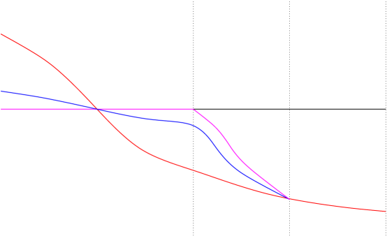
Figure 14. Schematic of $f_{40}$ (red), $\widehat{f}_{40}$ (purple), $f_{40}^{n}$ (blue).

Now take smooth functions

$$H_{n},G_{n}:M\longrightarrow\mathbb{R}\text{ so that }\phi_{1}^{H_{n}}(\Gamma(\widehat{f}_{40}))=\Gamma(df_{40}^{n}),\text{ and }\phi_{1}^{G_{n}}(L_{0})=\Gamma(df_{40}^{n}).$$

We may assume $H_{n}\longrightarrow 0$ in the $C^{\infty}$ norm, since $f_{40}^{n}\longrightarrow\widehat{f}_{40}$. Similarly we may assume $G_{n}\longrightarrow G$ such that $\phi_{1}^{G}(L_{0})=\Gamma(d\widehat{f}_{40})$. To be more definite, assume that in coordinates $(x,y)\in T^{*}L_{0}$ in some small Weinstein neighborhood of $L_{0}$ we have $H_{n}(x,y)=-(f_{40}^{*}(x)-f_{40}^{n}(x))$ and $G_{n}(x,y)=-f_{40}^{n}(x)$ (the signs in front are necessary because of our conventions in §13a).

Let $\widehat{V}_{4}$ and $V_{4}^{n}$ be the exact Lagrangian spheres obtained by replacing the graph $\Gamma(df_{40})$ by $\Gamma(d\widehat{f}_{40})$ and $\Gamma(df_{40}^{n})$ respectively.

Lemma 11.2.

Take any $J\in\mathcal{J}([0,1],M,I)$. Assume $J_{n}\in\mathcal{J}([0,1],M,I)$ satisfies $J_{n}\longrightarrow J$ in the $C^{\infty}$ sense. Then for any $\epsilon>0$ there is an $N$ such that for $n\geq N$, every

$$u\in\mathcal{M}(\widehat{V}_{4},V_{0},H_{n},J_{n};M)$$

has $Image(u)\subset\mathcal{N_{\epsilon}}(\widehat{N}_{40})=\{p\in M:dist(p,\widehat{N}_{40})<\epsilon\}$.

Proof.

Since $\phi_{H_{n}}(\widehat{V}_{4})$ has Morse-Bott intersection with $V_{0}$ it follows from condition 13.1 that every $u\in\mathcal{M}(\widehat{V}_{4},V_{0},H_{n},J_{n};M)$ satisfies

$$\lim_{s\longrightarrow\infty}u(s,\cdot)=y_{0},\phantom{bb}\lim_{s\longrightarrow-\infty}u(s,\cdot)=y_{1}$$

for some $y_{0},y_{1}\in C^{\infty}([0,1],M)$ such that, for $j=0,1$,

$$y_{j}^{\prime}(t)=X_{H_{n}}(y_{j}(t)),\,t\in[0,1],\phantom{bbb}y_{j}(0)\in\widehat{V}_{4},\,y_{j}(1)\in V_{0}.$$

Such $y_{j}$ are in one-one correspondence with points of

$$\phi_{H_{n}}(\widehat{V}_{4})\cap V_{0}=Crit(\frac{1}{n}f_{40})=Crit(f_{40}).$$

Since $dH_{n}(p)=0$ for any $p\in Crit(\frac{1}{n}f_{40})$, the $y_{j}$ are constant.

Now suppose for a contradiction that the lemma is false. Then, there is some $\epsilon>0$ and a sequence $u_{n}\in\mathcal{M}(\widehat{V}_{4},V_{0},H_{n},J_{n};M)$ such that for every $n$ the image of $u_{n}$ contains a point $x_{n}\notin\mathcal{N_{\epsilon}}(\widehat{N}_{40})$. Passing to subsequences, and reparameterizing each $u_{n}$ by a suitable $s_{n}\in\mathbb{R}$, we assume: $x_{n}\rightarrow x_{0}\notin\mathcal{N_{\epsilon}}(\widehat{N}_{40})$; $u_{n}(t_{n},0)=x_{n}$, for some $t_{n}\in[0,1]$, $t_{n}\rightarrow t_{0}$; there are fixed critical manifolds $C_{0},C_{1}$ of $\frac{1}{n}f_{40}$ such that for every $n$, $\lim_{s\rightarrow\infty}u_{n}(s,t)=y_{0}^{n}$, $\lim_{s\rightarrow-\infty}u(s,t)=y_{1}^{n}$, where $y_{0}^{n}\in C_{0}$, $y_{1}^{n}\in C_{1}$ $y_{0}^{n}\rightarrow y_{0}$, $y_{1}^{n}\rightarrow y_{1}$.

Because $M$ and the Lagrangian submanifolds are exact, $\int_{\mathbb{R}\times[0,1]}u_{n}^{*}\omega$ is uniformly bounded, and there is no bubbling. Hence, by Gromov compactness, there is a convergent subsequence $u_{n}\longrightarrow u$ where

(11.29) $$\partial_{s}u+J_{t}\partial_{t}u=0,$$

since $H_{n}\longrightarrow 0$. We also have $\lim_{s\rightarrow-\infty}u(s,t)=y_{0}$, $\lim_{s\rightarrow\infty}u(s,t)=y_{1}$, $u(t_{0},0)=x_{0}$. Let $f_{\widehat{V}_{4}}\in C^{\infty}(\widehat{V}_{4})$, $f_{V_{0}}\in C^{\infty}(V_{0})$ be such that $\theta|\widehat{V}_{4}=df_{\widehat{V}_{4}}$, $\theta|V_{0}=df_{V_{0}}$. We can assume $f_{\widehat{V}_{4}}$, $f_{V_{0}}$ to be equal to 0 on $Crit(\frac{1}{n}f_{40})$, since $\widehat{V}_{4}\cap\widehat{N}_{40}=\widehat{N}_{40}$ and $V_{0}\cap\widehat{N}_{40}=\widehat{N}_{40}$. This together with $H_{n}\longrightarrow 0$ shows that $\int_{\mathbb{R}\times[0,1]}u_{n}^{*}\omega=A(y_{1}^{n})-A(y_{0}^{n})\longrightarrow 0$. It follows that $\int_{\mathbb{R}\times[0,1]}u^{*}\omega=0$, and so by (11.29), $u$ must be constant, and equal to $u(t_{0},0)=x_{0}\notin\mathcal{N_{\epsilon}}(\widehat{N}_{40})$. On the other hand, since $u_{n}(t_{0},0)\in\widehat{V}_{4}$, and $u_{n}(t_{0},1)\in V_{0}$ both converge to $x_{0}$, it follows that $x_{0}\in\widehat{V}_{4}\cap V_{0}=\widehat{N}_{40}$, contradiction. ∎

Note that for $n$ sufficiently large we still have $||\nabla_{\mu_{40}}f_{40}^{n}||_{\infty}<A(L_{0},\mu_{40})$ (from the corresponding inequality for $f_{40}^{*}$).

Proposition 11.3.

For each $n$ there exist $J_{40}^{n}\in\mathcal{J}([0,1],M,I)$ such that $J_{40}^{n}$ converges to some $J_{40}^{\infty}\in\mathcal{J}([0,1],M,I)$ in the $C^{\infty}$ sense, and $J_{40}^{n}$ is such that for all $n$ sufficiently large we have for each $p,q\in Crit(f_{40})=Crit(\frac{1}{n}f_{40})$, a 1-1 correspondence between

$$\{\gamma\in C^{\infty}(\mathbb{R},N_{40}):\gamma^{\prime}(s)=(\frac{1}{n}\nabla_{\mu_{40}}f_{40})(\gamma(s)),\gamma(-\infty)=p,\gamma(\infty)=q\}$$

and $\mathcal{M}(V_{4}^{n},V_{0},J_{40}^{n},p,q;M).$ Namely the correspondence sends $\gamma$ to $u$, where $u(s,t)=\phi_{t}(\gamma(s)),$ and $\phi_{t}$, $t\in[0,1]$, is a certain exact isotopy which fixes $Crit(f_{40})$ point-wise. Finally, $J_{40}^{n}$ is regular for the second moduli space if and only if the first moduli space is regular.

Proof.

Unfortunately Floer’s proof does not work for the the case of a manifold with boundary. Instead, the idea is to appeal to Floer’s theorem for $L=L_{0},f=-f_{40}^{n}$, and then deduce from lemma 11.2 that, for large $n$, the corresponding result is true for $N_{40}$ and $f_{40}^{n}|N_{40}:N_{40}\longrightarrow\mathbb{R}$. (Since $f=-f_{40}^{n}$ we get a correspondence with positive flow lines of $f_{40}^{n}$.)

Let $J_{\mu_{40}}^{*}$ denote any extension of $J_{\mu_{40}}$ from a Weinstein neighborhood $D(T^{*}L_{0})$ to $M$ which is equal to $I$ near $\partial M$ (where $I$ makes $\partial M$ convex). Now set

$$J_{t}^{n}=(\phi^{H_{n}}_{t})_{*}(\phi^{H_{n}}_{1})^{*}(\phi^{G_{n}}_{1})_{*}(\phi^{G_{n}}_{t})^{*}(J_{\mu_{40}}^{*}).$$

Then $J_{t}^{n}\longrightarrow(\phi^{G}_{1})_{*}(\phi^{G}_{t})^{*}(J_{\mu_{40}}^{*})$ and we may assume $G_{n}$ is zero near $\partial M$, so that $J^{n}_{t}=I$ near $\partial M$. Note that

$$(\phi^{H_{n}}_{1})_{*}(\phi^{H_{n}}_{t})^{*}J_{t}^{n}=(\phi^{G_{n}}_{1})_{*}(\phi^{G_{n}}_{t})^{*}(J_{\mu_{40}})\text{ on }D(T^{*}N_{40}).$$

There are isomorphisms (see (13.37) in §13a),

$$\mathcal{M}(\widehat{V}_{4},V_{0},H_{n},\{J_{t}^{n}\},M)\cong\mathcal{M}(\widehat{V}_{4},(\phi^{H_{n}}_{1})^{-1}(V_{0}),\{(\phi^{H_{n}}_{t})^{*}J_{t}^{n}\},M)$$

$$\cong\mathcal{M}(\phi^{H_{n}}_{1}(\widehat{V}_{4}),V_{0},\{(\phi^{H_{n}}_{1})_{*}(\phi^{H_{n}}_{t})^{*}J_{t}^{n}\},M),$$

where the isomorphisms are respectively

$$u\mapsto\widetilde{u},\text{ }\widetilde{u}(s,t)=(\phi_{t}^{H_{n}})^{-1}(u(s,t)),\text{ and }\widetilde{u}\mapsto\phi_{1}^{H_{n}}(\widetilde{u}).$$

Now set

$$J_{40}^{n}=(\phi^{H_{n}}_{1})_{*}(\phi^{H_{n}}_{t})^{*}J_{t}^{n}.$$

We will now prove this satisfies conditions of the lemma (keeping in mind $\phi^{H_{n}}_{1}(\widehat{V}_{4})=V_{4}^{n}$). Let $\epsilon>0$ be such that $\mathcal{N}_{2\epsilon}(\widehat{N}_{40})\subset D(T^{*}N_{40})$. Lemma 11.2 implies that, for large $n$, each

$$u\in\mathcal{M}(\widehat{V}_{4},V_{0},H_{n},\{J^{n}_{t}\},M)$$

is contained in $\mathcal{N}_{\epsilon}(\widehat{N}_{40})$. Since $H_{n}\longrightarrow 0$ in $C^{1}$ we have, for large $n$,

$$(\phi_{1}^{H_{n}}\circ(\phi_{t}^{H_{n}})^{-1})(\mathcal{N}_{\epsilon}(\widehat{N}_{40}))\subset\mathcal{N}_{2\epsilon}(\widehat{N}_{40}),$$

for all $t$. Each

$$u\in\mathcal{M}(\phi^{H_{n}}_{1}(\widehat{V}_{4}),V_{0},\{(\phi^{H_{n}}_{1})_{*}(\phi^{H_{n}}_{t})^{*}J_{t}^{n}\},M)$$

therefore lies in $\mathcal{N}_{2\epsilon}(\widehat{N}_{40})\subset D(T^{*}N_{40})$ for large $n$. Therefore it follows that each such $u$ satisfies

$$u\in\mathcal{M}(\phi_{1}^{G_{n}}(L_{0}),L_{0},(\phi_{1}^{G_{n}})_{*}(\phi_{t}^{G_{n}})^{*}(-J_{g_{0}}),T^{*}L_{0}).$$

This is because $u$ lies in $D(T^{*}N_{40})$, and by construction the Lagrangians and complex structures are are equal in $D(T^{*}N_{40})$. Now Floer’s Theorem 11.1 applied to

$$\mathcal{M}(L_{0},L_{0},G_{n},J_{\mu_{40}},T^{*}L_{0})$$

implies that $u$ is of the form $u(s,t)=((\phi_{1}^{G_{n}})\circ(\phi_{t}^{G_{n}})^{-1})(\gamma(s))$ for some $\gamma\in C^{\infty}(\mathbb{R},L_{0})$ such that $\gamma^{\prime}(s)=(\nabla_{\mu_{40}}f_{40}^{n})(\gamma(s))$ (recall $G_{n}(x,y)=-f_{40}^{n}(x)$). Since $u$ lies in $D(T^{*}N_{40})$, we have $\lim_{s\longrightarrow\pm\infty}u(s,t)=x_{\pm}\in N_{40}$. Therefore, since $\phi_{t}^{G_{n}}(x)=x$ for all $x\in Crit(f_{40}^{n})$, $\gamma(\pm\infty)=x_{\pm}\in N_{40}.$ But the only gradient lines of $f_{40}^{n}$ joining points in $N_{40}$ are contained in $\widehat{N}_{40}$. Therefore, since $f_{40}^{n}|\widehat{N}_{40}=\frac{1}{n}f_{40}|\widehat{N}_{40}$ $\gamma$ in fact satisfies $\gamma\in C^{\infty}(\mathbb{R},N_{40})$, $\gamma^{\prime}(s)=(\nabla_{g_{0}}(\frac{1}{n}f_{40})(\gamma(s)).$

To address the statement about regularity we note that correspondence in Floer’s Theorem 11.1 has a version at the linearized level which carries regular data into regular data (see [P94, p. 86]). ∎

One can prove a version of lemmas 11.2 and 11.3 for $(V_{2}^{j},V_{0})$ and $(V_{4},V_{2}^{j})$ in the same way. The signs $\gamma^{\prime}(s)=-\frac{1}{n}(\nabla f_{42})(\gamma(s))$ and $\gamma^{\prime}(s)=-\frac{1}{n}(\nabla f_{20})(\gamma(s))$ in the correspondence are determined in the course of the argument. Alternatively, if $u\in\mathcal{M}(L_{0},L_{1},J)$, where $(L_{0},L_{1},J)=$ $(V_{4},V_{0},J_{40})$ or $(V_{4},V_{2}^{j},J_{42})$ or $(V_{2}^{j},V_{0},J_{20}^{j})$, then the corresponding action functionals satisfy

$$A_{20}(u(s,\cdot))=f_{20}^{j}(\pi(u(s,1))),\phantom{bbb}A_{42}(u(s,\cdot))=-f_{42}^{j}(\pi(u(s,0))),$$

$$A_{40}(u(s,\cdot))=-f_{40}^{j}(\pi(u(s,0))),$$

and $\partial_{s}A(u(s,\cdot))<0$ in all cases. Here $\pi:T^{*}N\longrightarrow N$ is the projection for $N=N_{42},N_{20},$ or $N_{40}$. The term in $A$ of the form $\int y^{*}\theta$ always vanishes because all $u$ are such that, for any fixed $s$, $y(t)=u(s,t)$ lies in a fixed cotangent fiber for all $t$.

12. Classification of holomorphic triangles in $D(T^{*}L_{2}^{j})$

In this section we prove Proposition 8.6, which corresponds here to Propositions 12.4 (existence), 12.9 (uniqueness), 12.10 (regularity), in sections 12a, 12b, 12c. (The arguments of this section are sketched in §4c and §4d.)

Take $Z=\{(z_{1},\ldots,z_{4})\in\mathbb{C}^{4}:\Sigma z_{j}^{2}=1\}$. This is exact symplectomorphic to $T^{*}S^{3}=\{(u,v)\in\mathbb{R}^{4}\times\mathbb{R}^{4}:|u|=1,u\cdot v=0\}$, via

$$\mu:Z\longrightarrow T^{*}S^{3},\phantom{bb}\mu(x+iy)=(x/|x|,-|x|y),\text{ where }\mu^{*}(\Sigma_{j}-v_{j}du_{j})=\Sigma_{j}\,y_{j}dx_{j}.$$

$Z$ has a complex structure $J_{Z}$, and we equip $T^{*}S^{3}$ with

(12.30) $$J_{\mathbb{C}}=\mu^{*}(J_{Z}).$$

The formula for $\mu^{-1}$ is

(12.31) $$\mu^{-1}(u,v)=f(|v|)u-if(|v|)^{-1}v,\phantom{bbb}f(s)=\sqrt{\frac{1+\sqrt{1+4s^{2}}}{2}}.$$

(This formula for $|x|=f(|v|)$ is obtained by combining the equations $|x|^{2}-|y|^{2}=1$ and $|x||y|=|v|$.)

As before we set $W_{4}^{j}=\widetilde{V}_{4}\cap D(T^{*}L_{2}^{j})$, $W_{2}^{j}=\widetilde{V}_{2}^{j}\cap D(T^{*}L_{2}^{j})$, $W_{0}^{j}=\widetilde{V}_{0}\cap D(T^{*}L_{2}^{j})$. For convenience of notation, we fix $j$ and consider $D(T^{*}L_{2}^{j})=D(T^{*}S^{3})$; we also drop the $j$ from $W_{4}^{j}$, $W_{2}^{j}$, $W_{0}^{j}$, and from $K_{\pm}^{j}$. Any $w\in\mathcal{M}(W_{4},W_{2},W_{0},J_{\mathbb{C}};D(T^{*}S^{3}))$ has a continuous extension to $D^{2}$, by condition 13.1, and we denote it by $\overline{w}:D^{2}\longrightarrow D(T^{*}S^{3}).$

12a. Existence of holomorphic triangles

For each $e\in K_{+}$, $f\in K_{-}$, let $Y_{ef}\subset Z$ denote the complex submanifold $Y_{ef}=(\mathbb{C}e\oplus\mathbb{C}f)\cap Z\subset\mathbb{C}^{4}.$

Lemma 12.1.

$\mu(Y_{ef})=T^{*}K_{ef}$, and there is a biholomorphism $\rho_{ef}:\mathbb{C}^{\times}\longrightarrow Y_{ef}.$

Proof.

To see $\mu(Y_{ef})=T^{*}K_{ef}$ we check that

$$\mu^{-1}(T^{*}K_{ef})\subset\{(z_{1}e,z_{2}f):z_{1}^{2}+z_{2}^{2}=1\}=Y_{ef},$$

using (12.31), and

$$\mu(Y_{ef})\subset[(\mathbb{R}e\oplus\mathbb{R}f)\oplus(\mathbb{R}e\oplus\mathbb{R}f)]\cap T^{*}S^{3}=T^{*}K_{ef}.$$

We define $\rho_{ef}:\mathbb{C}^{\times}\longrightarrow Y_{ef}$ by $\rho_{ef}(\zeta)=(z_{1}e,z_{2}f)$, where $z_{1}=\zeta+\zeta^{-1}$, $z_{2}=-i(\zeta-\zeta^{-1})$. Here, $z_{1}^{2}+z_{2}^{2}=(z_{1}+iz_{2})(z_{1}-iz_{2})=1,$ and $\zeta=z_{1}+iz_{2}$. ∎

We will need $\rho_{ef}$ because $\sigma_{ef}:(\mathbb{R}/2\pi\mathbb{Z})\times\mathbb{R}\longrightarrow T^{*}K_{ef}$ is unfortunately not holomorphic. We have the following refinement of the Riemann mapping theorem from [W92], Chapter 2, Theorems 2.1, 2.2, 2.4.

Lemma 12.2.

Assume $\Omega\subset\mathbb{C}$ is homeomorphic to a closed disk, and $\partial\Omega$ is parametrized by a continuous, injective curve $\gamma:\mathbb{R}/2\pi\mathbb{Z}\longrightarrow\partial\Omega$, which is piece-wise real analytic. Let $t_{0},t_{1},t_{2}\in\mathbb{R}/2\pi\mathbb{Z}$ denote three distinct points such that $\gamma|[(\mathbb{R}/2\pi\mathbb{Z})\setminus\{t_{0},t_{1},t_{2}\}]$ is real analytic. Let $z_{i}=\gamma(t_{i})$, and assume $z_{0},z_{1},z_{2}$ are labeled in counter-clockwise order. Let $l_{0}=\gamma(t_{0},t_{1}),l_{1}=\gamma(t_{1},t_{2}),l_{2}=\gamma(t_{2},t_{0})$. Then there is a unique biholomorphic map

$$w:V\longrightarrow\Omega\setminus\{z_{0},z_{1},z_{2}\}$$

such that

$$w(I_{i})=l_{i},\text{ and }\lim_{\zeta\rightarrow\zeta_{i}}w(\zeta)=z_{i},\,i=0,1,2.\,\square$$

We will need the following stronger version of lemma 12.2 for the uniqueness part because our holomorphic triangles $w:V\longrightarrow\Omega\setminus\{z_{0},z_{1},z_{2}\}$ would not be assumed to be injective, nor surjective on the boundary.

Lemma 12.3.

Take $\Omega$ as in lemma 12.2. Suppose $w:V\longrightarrow\Omega$ is holomorphic and

$$\lim_{\zeta\rightarrow\zeta_{i}}w(\zeta)=z_{i},\,i=0,1,2.$$

Taking $i,i+1$ modulo 3, assume that $w(I_{i})\subset\gamma(t_{i},t_{i+1})\text{, }i=0,1,2.$ Then $w:V\longrightarrow\Omega\setminus\{z_{0},z_{1},z_{2}\}$ is a biholomorphism, and it coincides with the map in lemma 12.2.

Proof.

Let $\overline{w}:D^{2}\longrightarrow\Omega$ denote the continuous extension of $w$. Let $b:\mathbb{R}/2\pi\mathbb{Z}\longrightarrow\partial D^{2}$ be $b(\theta)=e^{i\theta}$. Let $J_{i}\subset\mathbb{R}/2\pi\mathbb{Z}$, $i=0,1,2$ denote the open subintervals such that $b(J_{i})=I_{i}\subset V$. Then $(\overline{w}\circ b)|\overline{J}_{i}$ is a continuous curve connecting the point $z_{i}$ to $z_{i+1}$, where we take $i,i+1$ modulo 3. Since $w(I_{i})\subset\gamma(t_{i},t_{i+1})$, we conclude $(w\circ b)(\overline{J}i)=\gamma([t_{i},t_{i+1}]).$ In total $(\overline{w}\circ b):\mathbb{R}/2\pi\mathbb{Z}\longrightarrow\partial D^{2}$ winds once around the boundary of $\Omega$ in the counter-clockwise sense, since $z_{0},z_{1},z_{2}$ are so ordered. So, for any $w_{0}\in\textup{Int\,}\Omega$,

$$\frac{1}{2\pi i}\int_{0}^{2\pi}\frac{(w\circ b)^{\prime}(t)}{(w\circ b)(t)-w_{0}}dt=1,$$

where $(w\circ b)^{\prime}(t)$ exists for all but finitely many $t$. This integral is also the number of zeros of $w(z)-w_{0}$ in $\textup{Int\,}D^{2}$ counted with multiplicity, so we conclude that

$$w|\textup{Int\,}D^{2}:\textup{Int\,}D^{2}\longrightarrow\textup{Int\,}\Omega$$

is a biholomorphic map. Let $\widetilde{w}$ denote the map from lemma 12.2. Since $(\widetilde{w}^{-1}\circ w)|\textup{Int\,}D^{2}$ is a biholomorphism of $\textup{Int\,}(D^{2})$ onto itself, it must be a linear fractional transformation, which extends to $\mathbb{C}$ and fixes $\zeta_{0}$, $\zeta_{1}$ $\zeta_{2}$. Thus $w=\widetilde{w}$. ∎

Let $\Delta\subset\mathbb{R}/2\pi\mathbb{Z}\times[-r,r]$ denote any one of the four triangles bounded by $\widetilde{\Gamma}_{0}$, $\widetilde{\Gamma}_{2}$, $\widetilde{\Gamma}_{4}$ in figure 6. Let $\delta_{42},\delta_{20},\delta_{40}$ denote the vertices of $\Delta$, where $\delta_{ij}\in\widetilde{\Gamma}_{k}\cap\widetilde{\Gamma}_{i}$, $k,i=0,2,4$. Set $\Delta^{*}=\Delta\setminus\{\delta_{42},\delta_{20},\delta_{40}\}.$

Proposition 12.4.

For each $e\in K_{+},f\in K_{-}$ there is a

$$w=w_{ef}\in\mathcal{M}(W_{4},W_{2},W_{0},J_{\mathbb{C}};D(T^{*}S^{3}))$$

satisfying

$$w_{ef}(V)=\sigma_{ef}(\Delta^{*})\subset D(T^{*}K_{ef}),$$

$$\lim_{\zeta\rightarrow\zeta_{0}}w(\zeta)=\sigma_{ef}(\delta_{40}),\,\,\lim_{\zeta\rightarrow\zeta_{1}}w(\zeta)=\sigma_{ef}(\delta_{20}),\,\,\lim_{\zeta\rightarrow\zeta_{2}}w(\zeta)=\sigma_{ef}(\delta_{42}).$$

Proof.

Let $\Delta^{\prime}=\rho_{ef}^{-1}(\mu^{-1}(\sigma_{ef}(\Delta)))\subset\mathbb{C}^{\times}.$ First we check that the boundary arcs of $\Delta^{\prime}$ are real analytic. A calculation yields

$$(\rho_{ef}^{-1}\circ\mu^{-1}\circ\sigma_{ef})(\theta,s)=(f(s)+\frac{s}{f(s)})e^{i\theta}.$$

Recall from formula (12.31) that

$$f(s)=\sqrt{\frac{1+\sqrt{1+4s^{2}}}{2}}\geq 1.$$

Thus $s\mapsto f(s)+\frac{s}{f(s)}$ is real analytic on all of $\mathbb{R}$. By construction $\Delta$ (see §8) has real analytic boundary arcs, therefore $\Delta^{\prime}$ does as well.

Note that $I_{0},I_{1},I_{2}$ label the boundary arcs of $V$ in counter-clockwise order, whereas $\Gamma_{0},\Gamma_{2},\Gamma_{4}$ label the boundary arcs of $\Delta$ in clockwise order. We claim that

$$\rho_{ef}^{-1}\circ\mu^{-1}\circ\sigma_{ef}:\mathbb{R}/2\pi\mathbb{Z}\times\mathbb{R}\longrightarrow\mathbb{C}^{\times}$$

is orientation reversing: $(\rho_{ef}^{-1}\circ\mu^{-1}\circ\sigma_{ef})^{*}(d\tilde{x}\wedge d\tilde{y})=-d\theta\wedge d\lambda,$ where $\tilde{x}+i\tilde{y}\in\mathbb{C}^{\times}$, $(\theta,\lambda)\in\mathbb{R}/2\pi\mathbb{Z}\times\mathbb{R}$. To see this note that, since $\rho_{ef}^{-1}$ is a biholomorphism, it respects the orientations of $(\Sigma_{j}\,dx_{j}\wedge dy_{j})|Y_{ef})$ and $d\tilde{x}\wedge d\tilde{y}$ on $\mathbb{C}^{\times}$, where $(x_{j}+iy_{j})\in\mathbb{C},$ $j=1,\ldots,4$. Then one calculates:

$$(\mu^{-1})^{*}(\Sigma_{j}\,dx_{j}\wedge dy_{j})=(\Sigma_{j}\,dv_{j}\wedge du_{j}),\phantom{bbb}\sigma_{ef}^{*}(\Sigma_{j}\,dv_{j}\wedge du_{j})=-d\theta\wedge d\lambda,$$

where $(u,v)\in\mathbb{R}^{4}\times\mathbb{R}^{4}$ are the the usual coordinates for $T^{*}S^{3}$. Therefore

$$(\rho_{ef}^{-1}\circ\mu^{-1}\circ\sigma_{ef})(\Gamma_{0}),\,(\rho_{ef}^{-1}\circ\mu^{-1}\circ\sigma_{ef})(\Gamma_{2}),\,(\rho_{ef}^{-1}\circ\mu^{-1}\circ\sigma_{ef})(\Gamma_{4})$$

label the boundary arcs of $\Delta^{\prime}$ in counter-clockwise order. Then lemma 12.2 produces a biholomorphic map $\varphi:V\longrightarrow\Delta^{\prime}$ satisfying suitable boundary conditions, and we set $w_{ef}=\mu\circ\rho_{ef}\circ\varphi$. ∎

12b. Uniqueness of holomorphic triangles

Define

$$P:Z\longrightarrow\mathbb{C},\phantom{bbb}P(z_{1},z_{2},z_{3},z_{4})=z^{2}_{1}+z_{2}^{2}-z_{3}^{2}-z_{4}^{2}.$$

Set $Y=\{(w_{1},w_{2})\in\mathbb{C}^{2}:w_{1}^{2}+w_{2}^{2}=1\}\cong T^{*}S^{1}$.

Lemma 12.5.

Let $U\subset\mathbb{C}\setminus\{\pm 1\}$ be such that the map induced by the inclusion $\pi_{1}(U)\longrightarrow\pi_{1}(\mathbb{C}\setminus\{\pm 1\})$ is trivial. Then there is a holomorphic trivialization of $P:Z\longrightarrow\mathbb{C}$ over $U$ given by

$$\Phi:P^{-1}(U)\longrightarrow U\times Y\times Y,\phantom{bbb}\Phi(z_{1},z_{2},z_{3},z_{4})=(\lambda,\alpha(\lambda)(z_{1},z_{2}),\beta(\lambda)(z_{3},z_{4})),$$

where $\lambda=P(z_{1},z_{2},z_{3},z_{4})$, and $\alpha,\beta:U\longrightarrow\mathbb{C}$ are the following holomorphic functions.

$$\alpha(\lambda)=\sqrt{\frac{2}{1+\lambda}},\lambda\in U,\phantom{bbb}\beta(\lambda)=\sqrt{\frac{2}{1-\lambda}},\lambda\in U.$$

(Here we have chosen branches of the square root function.)

Proof.

Assume $z\in P^{-1}(\lambda)$ for some $\lambda\in\mathbb{C}$. Then

$$z^{2}_{1}+z_{2}^{2}-z_{3}^{2}-z_{4}^{2}=\lambda,\,\,z_{1}^{2}+z_{3}^{2}+z_{4}^{2}+z_{4}^{2}=1,$$

since the domain of $P$ is $Z$. Therefore

$$z_{1}^{2}+z_{2}^{2}=\frac{1+\lambda}{2},\phantom{bbb}z_{3}^{2}+z_{4}^{2}=\frac{1-\lambda}{2}.$$

Now, by the assumptions on $U$, $\{\frac{2}{\lambda+1}:\lambda\in U\}$ and $\{\frac{2}{\lambda-1}:\lambda\in U\}$ are subsets of $\mathbb{C}\setminus\{0\}$ and neither of them contains a nontrivial loop around 0. Therefore they both admit a branch of the square root function, and we can define $\alpha,\beta$ as stated. ∎

Let $B_{1},B_{2}\subset\mathbb{R}/2\pi\mathbb{Z}\times[-r,r]$ denote the two bigons adjacent to $\Delta$ bounded respectively by $\widetilde{\Gamma}_{4}$, $\widetilde{\Gamma}_{2}$, and $\widetilde{\Gamma}_{2}$, $\widetilde{\Gamma}_{0}$ in figure 7 (where each $B_{i}$ has one vertex in common with $\Delta$).

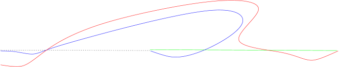
Figure 15. The curves $P(\mu^{-1}(W_{4}))$ (red), $P(\mu^{-1}(W_{2}))$ (green), $P(\mu^{-1}(W_{0}))$ (blue) in $\mathbb{C}$.

Lemma 12.6.

$P(\mu^{-1}(W_{0})),P(\mu^{-1}(W_{2})),P(\mu^{-1}(W_{4}))\subset\mathbb{C}$ are embedded curves in $\mathbb{C}$ as in figure 15. They enclose three compact regions $R$, $R_{1}$, $R_{2}$, Here, $R_{1},R_{2}\subset\{z\in\mathbb{C}:Imz\leq 0\}$ are bigons diffeomorphic to $B_{1}$, $B_{2}$, and $R$ is a triangular region, diffeomorphic to $\Delta$, which is contained in

$$(\mathbb{C}\setminus\{-1,1\})\cap\{z\in\mathbb{C}:Im\,z\geq 0\}.$$

In particular $U=R$ satisfies the assumptions of the last lemma.

Proof.

A computation shows that

(12.32) $$P(\mu^{-1}(\sigma_{ef}(\theta,\lambda)))=\sqrt{1+4\lambda^{2}}\cos 2\theta+i2\lambda\sin 2\theta.$$

Indeed, $P(\mu^{-1}(\sigma_{ef}(\theta,\lambda)))$ is equal to

$$P\big{(}f(\lambda)(\cos(\theta)e,\sin(\theta)f)+i(-\frac{\lambda}{f(\lambda)})(-\sin(\theta)e,\cos(\theta)f)\big{)}$$

$$=(f(\lambda)^{2}+f(\lambda)^{-2}\lambda^{2})\cos 2\theta+2i\lambda\sin 2\theta.$$

Set

$$a(\lambda)=f(\lambda)^{2}+f(\lambda)^{-2}\lambda^{2},\phantom{bbb}b(\lambda)=2\lambda,$$

and recall from (12.31) that $f(\lambda)$ satisfies

$$(f(\lambda)^{2})^{2}-f(\lambda)^{2}-\lambda^{2}=0.$$

Hence

$$f(\lambda)^{2}a(\lambda)=(f(\lambda)^{2})^{2}+\lambda^{2}=f(\lambda)^{2}+2\lambda^{2}\text{, and}$$

$$a(\lambda)=1+2\frac{\lambda^{2}}{f(\lambda)^{2}}=1+4\frac{\lambda^{2}}{1+\sqrt{1+4\lambda^{2}}}=1+(\sqrt{1+4\lambda^{2}}-1).$$

Formula (12.32) implies

$$p=P\circ\mu^{-1}\circ\sigma_{ef}:\mathbb{R}/2\pi\mathbb{Z}\times[-r,r]\longrightarrow\mathbb{C}$$

is independent of $e,f$. Therefore, it is enough to describe the images of $\widetilde{\Gamma}_{4}$, $\widetilde{\Gamma}_{2}$, $\widetilde{\Gamma}_{0}$ under $p$. Note also that the formula for $p$ is periodic, so it suffices to understand $p$ just near $\Delta$; the other three triangles are mapped onto $p(\Delta)$ as well. One can understand the map $p$ as follows. For fixed $\lambda>0$, we have $a(\lambda)>0$ and $b(\lambda)>0$; thus as $\theta$ ranges from $0$ to $\pi$,

$$\theta\mapsto p(\theta,\lambda)=a(\lambda)\cos 2\theta+ib(\lambda)\sin 2\theta$$

parameterizes an ellipse in the counterclockwise direction, with axes $a(\lambda)$ and $b(\lambda)i$. Now as $\lambda>0$ varies, one gets a family of disjoint ellipses, since $a,b$ are strictly increasing functions. Similarly, for fixed $\lambda<0$, we have $a(\lambda)>0$, $b(\lambda)<0$, so one gets an ellipse parameterized in the clockwise direction. For $\lambda=0$, we get the map $\theta\mapsto\cos(2\theta)+0i$. Using this description of $p$, we sketch $P(\mu^{-1}(W_{0}))=p(\widetilde{\Gamma}_{0}),$ $P(\mu^{-1}(W_{2}))=p(\widetilde{\Gamma}_{2}),$ $P(\mu^{-1}(W_{4}))=p(\widetilde{\Gamma}_{4})$ as in figure 15. ∎

Lemma 12.7.

Let $w\in\mathcal{M}(W_{4},W_{2},W_{0},J_{\mathbb{C}};D(T^{*}S^{3}))$ and denote its continuous extension by $\overline{w}:D^{2}\longrightarrow D(T^{*}S^{3}))$. Then $P(\mu^{-1}(\overline{w}(D^{2})))=R.$

Proof.

For this proof we consider $\mu^{-1}\circ\overline{w},\mu^{-1}\circ w:V\longrightarrow Z$, but we denote them again by $\overline{w},w$. The lemma follows basically from the maximum principle. Let $R,R_{1},R_{2}$ be as in the last lemma (see figure 15). Let $p_{40}$, $p_{42}$, and $p_{20}$ denote the vertices of $R$, let $q_{42}$ and $p_{42}$ denote the two vertices of $R_{1}$, and let $q_{20}$ and $p_{20}$ denote those of $R_{2}$. Then, the boundary conditions on $w$, plus the description of $P(\mu^{-1}(W_{4}))$, $P(\mu^{-1}(W_{2}))$, $P(\mu^{-1}(W_{0}))$ in the last lemma imply

$$P(\overline{w}(\zeta_{0}))=p_{40},\,\,P(\overline{w}(\zeta_{1}))=p_{42}\text{ or }q_{42},\,\,P(\overline{w}(\zeta_{2}))=p_{20}\text{ or }q_{20}.$$

Let $D=R_{1}\cup R\cup R_{2}$ and $D^{\prime}=D\cup P(W_{2})\cup P(W_{4})$. Assume for a contradiction there exists $\zeta\in D^{2}$ such that $(P\circ\overline{w})(\zeta)\notin D^{\prime}$. Let $C:[0,\infty)\longrightarrow\mathbb{C}\setminus D^{\prime}$ be a continuous curve such that $C(0)=(P\circ\overline{w})(\zeta)$ and $\lim_{t\rightarrow\infty}|C(t)|=\infty$. Let $t_{max}$ be the largest element of the compact set $C^{-1}[(P\circ\overline{w})(D^{2})]$. Let $\zeta_{max}\in D^{2}$ be such that $(P\circ\overline{w})(\zeta_{max})=C(t_{max})\in\mathbb{C}\setminus D^{\prime}$. Now $\zeta_{max}$ is necessarily in the interior of $D^{2}$ because of the boundary conditions on $w$. But then, since $(P\circ w)|\textup{Int\,}D^{2}$ is a nonconstant holomorphic function, there must be an open disk around $(P\circ w)(\zeta_{max})$ contained in $(P\circ w)(\textup{Int\,}D^{2})$. Then by continuity of $C$ there must exist $t>t_{max}$ such that $C(t)\in(P\circ\overline{w})(D^{2})$, contradiction. Therefore $(P\circ\overline{w})(D^{2})\subset D^{\prime}$.

It follows easily that $(P\circ\overline{w})(D^{2})\subset D$, because if $\zeta\in D^{2}$ is such that $(P\circ\overline{w})(\zeta)\in D^{\prime}\setminus D$ then by continuity there is a nearby point $\zeta^{\prime}\in\textup{Int\,}(D^{2})$ satisfying the same condition; then a small neighborhood of $\zeta^{\prime}$ would map onto an open disk in $\mathbb{C}$, but this is impossible since $D^{\prime}\setminus D$ is contains no open disks.

Now suppose for a contradiction that there exists $\zeta\in D^{2}$ such that $P(\overline{w}(\zeta))\in R_{1}\setminus\{p_{42}\}$. Let $\upsilon:[0,1]\longrightarrow D^{2}$ be a path connecting $\zeta$ and $\zeta_{0}$ such that $\upsilon(0,1)\subset\textup{Int\,}(D^{2})$. Then by connectedness there is $\zeta^{\prime}\in\textup{Int\,}(D^{2})$ satisfying $P(\overline{w}(\zeta^{\prime}))=p_{42}.$ But there is no open disk contained around $p_{42}$ contained in $D$, so this is impossible. We conclude that $P(\overline{w}(D^{2}))\subset R\cup R_{2}$ and a similar argument implies $P(\overline{w}(D^{2}))\subset R$. The same type of argument, using the fact that $(P\circ w)|\textup{Int\,}D^{2}$ is an open map, shows that $P(\mu^{-1}(\overline{w}(D^{2})))=R$. ∎

Recall $Y=\{(w_{1},w_{2})\in\mathbb{C}^{2}:w_{1}^{2}+w_{2}^{2}=1\}\cong T^{*}S^{1}$ and set $L=\mathbb{R}^{2}\cap Y=S^{1}$. Lemmas 12.6 and 12.5 imply there is a holomorphic trivialization

(12.33) $$\Phi:P^{-1}(R)\longrightarrow R\times Y\times Y$$

Denote the compositions of $\Phi$ with the two projections to $Y$ by

(12.34) $$\Phi_{1},\Phi_{2}:P^{-1}(R)\longrightarrow Y.$$

Lemma 12.8.

For any $p\in\mu^{-1}(T^{*}K_{e^{\prime}f^{\prime}})\cap P^{-1}(R)$, we have $\Phi_{1}(p)=\pm e$ and $\Phi_{2}(p)=\pm f$, where $e^{\prime}=(e,0)\in K_{+}$, $f^{\prime}=(0,f)\in K_{-}$. Consequently,

$$\Phi_{\ell}(\mu^{-1}(W_{i})\cap P^{-1}(R))\subset L_{i}.$$

for any $\ell=1,2$, $i=0,2,4$

Proof.

By (12.31), every $p\in\mu^{-1}(T^{*}K_{e^{\prime}f^{\prime}})$ is of the form $p=(ae,bf),$ for some $a,b\in\mathbb{C}$. If $p\in\mu^{-1}(T^{*}K_{e^{\prime}f^{\prime}})\cap\Phi^{-1}(R)$, then

$$\Phi_{1}(p)=\alpha(\lambda)(ae)=\rho_{1}e\in Y,\,\,\Phi_{2}(p)=\beta(\lambda)(bf)=\rho_{2}f\in Y$$

for some $\rho_{1},\rho_{2}\in\mathbb{C}$. Since $\rho_{1}e,\rho_{2}f\in Y$ we have $\rho_{1}^{2}(e_{1}^{2}+e_{2}^{2})=\rho_{1}^{2}=1$, and similarly $\rho_{2}^{2}=1$. Thus $\rho_{1}=\pm 1,\rho_{2}=\pm 1.$ ∎

Proposition 12.9.

Every $w\in\mathcal{M}(W_{4},W_{2},W_{0},J_{\mathbb{C}};D(T^{*}S^{3}))$ is equal to $w_{ef}$ for some $e,f$, as in Proposition 12.4.

Proof.

Let $\overline{w}:D^{2}\longrightarrow T^{*}S^{3}$ be the continuous extension of $w$. Lemma 12.7 implies $R=P(\mu^{-1}(\overline{w}(D^{2})))$, and therefore it makes sense to form

$$\overline{w}_{k}=\Phi_{k}\circ\mu^{-1}\circ\overline{w}:D^{2}\longrightarrow Y,\,k=1,2.$$

Set $w_{k}=\Phi_{k}\circ\mu^{-1}\circ w.$ Then

$$w_{k}\in\mathcal{M}(L,L,L,J_{Y};Y),$$

where $J_{Y}$ is the complex structure from $\mathbb{C}^{2}$. Here, the boundary conditions follow from Lemma 12.8, and $\int_{V}w_{k}^{*}\omega_{Y}<\infty$ follows from the fact that $w_{k}$ has a continuous extension $\overline{w}_{k}$. Once we know $\int_{V}w_{k}^{*}\omega_{Y}<\infty$, we can apply Stokes’ theorem to compute $\int_{V}w_{k}^{*}\omega_{Y}$ in terms of $\theta_{Y}|L$; then, since $\theta_{Y}|L=0$, $\int_{V}w_{k}^{*}\omega_{Y}$ is zero and $w_{k}$ must be constant, say $w_{1}=e$, $w_{2}=f$.

Now, by lemma 12.6, $\Omega=R$ satisfies the assumptions of lemma 12.2. Further, $P\circ\mu^{-1}\circ w:V\longrightarrow R$ is holomorphic and maps $I_{0}$, $I_{1}$, $I_{2}$ into the corresponding boundary arcs of $R$ and $\zeta_{0}$, $\zeta_{1}$, $\zeta_{2}$ to the vertices of $R$ (see the proof of lemma 12.6). Hence, by lemma 12.3, it must be the unique biholomorphism $\psi:V\longrightarrow R$ satisfying these conditions. Choosing $e^{\prime}=(\pm e,0),f^{\prime}=(0,\pm f)$ suitably, $w_{e^{\prime}f^{\prime}}$ will also satisfy

$$\Phi_{1}\circ\mu^{-1}\circ w_{e^{\prime}f^{\prime}}=e,\phantom{bbb}\Phi_{2}\circ\mu^{-1}\circ w_{e^{\prime}f^{\prime}}=f$$

(the sign of $\pm e,\pm f$ depends on the choice of square-roots for $\alpha,\beta$). And, again, $P\circ\mu^{-1}\circ w_{e^{\prime}f^{\prime}}=\psi$. Therefore $w(\zeta)=\Phi^{-1}(\psi(\zeta),\pm e,\pm f)=w_{e^{\prime}f^{\prime}}(\zeta).$ ∎

12c. Regularity of the moduli space of holomorphic triangles

For this section we will work with $Z$ rather than $T^{*}S^{3}$, and we will look at the corresponding moduli space of $J$-holomorphic triangles, where $J=J_{Z}$,

$$\mathcal{M}=\mathcal{M}(\widetilde{W}_{4},\widetilde{W}_{2},\widetilde{W}_{0},J;Z),$$

where we set $\widetilde{W}_{i}=\mu^{-1}(W_{j}),\,i=0,2,4.$ As we explain in §13j, $\mathcal{M}$ sits inside a certain Banach space $\mathcal{B}$: there is a Banach-bundle $\mathcal{E}\longrightarrow\mathcal{B}$; the Cauchy-Riemann operator is a section $\partial_{J}:\mathcal{B}\longrightarrow\mathcal{E}$, and $\mathcal{M}=\partial_{J}^{-1}(0)$. For each $w\in\mathcal{M}$ the linearization $D(\overline{\partial}_{J})_{w}:T_{w}\mathcal{B}\longrightarrow\mathcal{E}_{w}$ is a Fredholm operator by lemma 13.3.

Proposition 12.10.

$J=J_{Z}$ is a regular almost complex structure. That is, for any $w\in\mathcal{M}$, the linearized operator $D(\overline{\partial}_{J})(w):T_{w}(\mathcal{B})\longrightarrow\mathcal{E}_{w}$ is surjective.

This follows from lemmas 12.13 and 12.14 below, which show that

$$\textup{dim}Ker(D(\overline{\partial}_{J})(w)=2\text{ and }\textup{index\,}D(\overline{\partial}_{J})(w)=2.$$

Remark 12.11.

In general, if $\textup{dim}N=2k$ and $\textup{dim}M=4k-2$, then the $2$ here will be $2k-2$. This is because $L_{0}\cong S^{2k-1}$, $K_{j}\cong S^{k-1}\cong K_{-}^{j}\cong K_{+}^{j}$, and then $2k-2=\textup{dim}\,\partial\mathcal{N}_{S^{2k-1}}(K_{j}^{\pm})$.

For the proof of lemma 12.13 we will need a special case of [S08, lemma 11.5], as stated in lemma 12.12 below. We first set up some notation. Take $E=\mathbb{C}\times V\longrightarrow V$ to be the trivial Hermitian line bundle over $V$. Let $F\longrightarrow\partial V$ be a totally real sub-bundle of $E|\partial V$. We define the winding number of $F$ as follows. Recall from §13f that $\zeta_{0}$, $\zeta_{1}$, $\zeta_{2}$ label the three punctures in counter clockwise order and $I_{0}$, $I_{1}$, $I_{2}$ label the boundary components of $\partial V$ in counter clockwise order, where $\zeta_{0}$, $\zeta_{1}$ lie on the boundary of $I_{0}$. We have fixed (incoming) strip-like ends

$$\epsilon_{0},\epsilon_{1}:(-\infty,0]\times[0,1]\longrightarrow V$$

parameterizing a neighborhood of $\zeta_{0}$ and $\zeta_{1}$, and we have an (outgoing) strip-like end at $\zeta_{2}$:

$$\epsilon_{2}:[0,\infty)\times[0,1]\longrightarrow V.$$

We assume $F$ is nondegenerate in the sense that $F_{\epsilon_{\zeta_{j}}(0,s)}$ and $F_{\epsilon_{\zeta_{j}}(1,s)}$ are transverse for $|s|>>0$ (where $s\in[0,\infty)$ if $j=2$ or $s\in(-\infty,0]$ if $j=0,1$). Now, we define a homotopy between $F_{\epsilon_{\zeta_{j}}(0,s)}$ and $F_{\epsilon_{\zeta_{j}}(1,s)}$ as follows. For convenience of notation, let us rotate $\epsilon_{j}^{*}(E)$ by a constant so that

$$F_{\epsilon_{\zeta_{j}}(0,s)}=\mathbb{R},\,F_{\epsilon_{\zeta_{j}}(1,s)}=e^{i\sigma_{j}}\mathbb{R}$$

for some $\sigma_{j}\in(-\pi,0)$. In that notation we take the homotopy which goes through

(12.35) $$e^{it\sigma_{j}},\,t\in[0,1]$$

Consider the compactification of $V$ to $\widehat{V}\cong D^{2}$ where we glue on a copy of the upper half plane at each puncture and use the homotopy (12.35) near each puncture. Let $\rho:S^{1}\longrightarrow\mathbb{R}P^{1}$ denote the map we obtain in this way and let $\mu(\rho)\in\mathbb{Z}$ denote its degree; this is called the winding number of $F$. Let $|V^{-}|$ denote the number of incoming punctures of $V$, which in our case is 2. Let $\overline{\partial}$ denote the usual Cauchy-Riemann operator on $V\subset\mathbb{C}$, so $\overline{\partial}=\partial_{s}+i\partial_{t}$ in the coordinates $s+it\in\mathbb{C}$. We regard $\overline{\partial}$ as operating on sections of $E$ with boundary in $F$.

Lemma 12.12.

If $\mu(\rho)-|V^{-}|=\mu(\rho)-2<0$ then $Ker(\overline{\partial})=\{0\}$.  $\square$

For the proof see [S08, lemma 11.5].

Lemma 12.13.

For any $w\in\mathcal{M}$, $dim(KerD(\overline{\partial}_{J})(w))=2$.

Proof.

Fix $w\in\mathcal{M}$. By condition 13.1 $w$ has a continuous extension to $D^{2}$, which we denote $\overline{w}:D^{2}\longrightarrow Z$. Since $J$ is the restriction of the usual complex structure on $\mathbb{C}^{4}$, we have $D(\overline{\partial}_{J})(w)(X)=\overline{\partial}X$, where $\overline{\partial}$ is the usual Cauchy-Riemann operator acting on $C^{\infty}(\mathbb{C},\mathbb{C}^{4}).$ Thus, each $X\in KerD(\overline{\partial}_{J})(w)$ is a holomorphic map $X:V\longrightarrow\mathbb{C}^{4}$. By definition of $T_{w}(\mathcal{B})$, it has a continuous extension $\overline{X}:D^{2}\longrightarrow\mathbb{C}^{4}$. This satisfies

$$\overline{X}(\zeta)\in T_{\overline{w}(\zeta)}Z=\{(z_{1},z_{2},z_{3},z_{4})\in\mathbb{C}^{4}:\Sigma_{i}z_{i}\overline{w}_{i}(\zeta)=0\}\text{ for all }\zeta\in D^{2},$$

$$\overline{X}(\zeta)\in T_{\overline{w}(\zeta)}(\widetilde{W}_{2k}),\text{ for all }\zeta\in\overline{I}_{k}\subset\partial D^{2},k=0,1,2.$$

Since $w\in\mathcal{M}(\widetilde{W}_{4},\widetilde{W}_{2},\widetilde{W}_{0},J_{Z})$, we have the holomorphic trivialization (12.33) over $R=P(\overline{w}(D^{2}))$

$$\Phi:P^{-1}(R)\longrightarrow R\times Y\times Y,$$

and projections (12.34),

$$\Phi_{1},\Phi_{2}:P^{-1}(R)\longrightarrow Y.$$

The rough idea for computing the kernal is to decompose a given $X$ using the trivialization $\Phi$:

$$X\mapsto(DP(X),(D\Phi_{1})(X),(D\Phi_{1})(X))$$

and then check that the first component is zero, while the last two components are constant and each lie in a one dimensional linear space.

Define

$$\overline{\varphi}:D^{2}\longrightarrow\mathbb{C},\phantom{bbb}\overline{\varphi}(\zeta)=DP_{\overline{w}(\zeta)}(\overline{X}(\zeta)).$$

Then $\varphi=\overline{\varphi}|V:V\longrightarrow\mathbb{C}$ is holomorphic and has a continuous extension to $D^{2}$, and

(12.36) $$\varphi(\zeta)\in T_{\varphi(\zeta)}(P(W_{2k})),\text{ for each }\zeta\in I_{k}\subset\partial D^{2},\,k=0,1,2.$$

We will show $\varphi$ is identically 0.

Recall $R=P(\overline{w}(D^{2}))$. The proof of lemma 12.6 shows that

$$P(\widetilde{W}_{2k})\cap R=p(\widetilde{\Gamma}_{2k}\cap\Delta)\text{ where}$$

$$p(\theta,\lambda)=\sqrt{1+4\lambda^{2}}\cos 2\theta+i2\lambda\sin 2\theta.$$

See figure 15. Now, let us regard $\varphi:V\longrightarrow\mathbb{C}$ as a section of the trivial Hermitian line bundle $E=V\times\mathbb{C}$ satisfying the totally real boundary conditions $F\longrightarrow\partial V$ given by (12.36). Since $F_{\epsilon_{j}(s,0)}$ and $F_{\epsilon_{j}(s,1)}$ are transverse at each puncture for $|s|>>0$, we can apply lemma 12.12 above to $(E,F,\overline{\partial})$. Since $\varphi$ has a continuous extension to $D^{2}$, it has finite energy and therefore it lies in the domain of $\overline{\partial}$ (which is the Sobolev space $W^{1,p}(V,E,F)$, $p>2$). We claim that the winding number of $F$, i.e. $\mu(\rho)\in\mathbb{Z}$, is equal to zero. Thus by lemma 12.12, $Ker(\overline{\partial})=\{0\}$ and so $\varphi$ is identically zero.

Indeed, $\mu(\rho)=0$ follows from inspection of figure 15, where we use the homotopies at the punctures given by (12.35). Note that the strip-like ends label each puncture as follows: The two boundary arcs at each of the two bottom vertices (i.e. the two punctures on the boundary of the arc $P(\mu^{-1}(W_{2}))$) will be labeled $1,0$ and $1,0$ in counter-clockwise order; the other vertex will be labeled $0,1$ in counter-clockwise order. (Roughly speaking, then, we have the following: The arc $P(\mu^{-1}(W_{0}))$ contributes $+1$ to the winding number; the arc along $P(\mu^{-1}(W_{2}))$ of course contributes nothing to the winding number, but the two punctures between $P(\mu^{-1}(W_{0}))$, $P(\mu^{-1}(W_{2}))$ and between $P(\mu^{-1}(W_{2}))$, $P(\mu^{-1}(W_{4}))$ together contribute $-1$ to the winding number; finally, the arc $P(\mu^{-1}(W_{4}))$ and the puncture between $P(\mu^{-1}(W_{4}))$ and $P(\mu^{-1}(W_{0}))$ contribute nothing to the winding number.)

For the other two components, let

$$\overline{\varphi}_{1}(\zeta)=(D_{\overline{w}(\zeta)}\Phi_{1})(\overline{X}(\zeta)),\,\phantom{bb}\overline{\varphi}_{2}(\zeta)=(D_{\overline{w}(\zeta)}\Phi_{2})(\overline{X}(\zeta)),\text{ for each }\zeta\in D^{2}.$$

Then

$$\varphi_{1}=\overline{\varphi}_{1}|V,\phantom{b}\varphi_{2}=\overline{\varphi}_{2}|V:V\longrightarrow\mathbb{C}^{2}$$

are holomorphic maps with continuous extensions to $D^{2}$ and, setting $\overline{w}_{j}=\Phi_{j}\circ\overline{w}$, we have

$$\overline{\varphi}_{1}(\zeta)\in T_{\overline{w}_{1}(\zeta)}(Y)\subset\mathbb{C}^{2},\text{ for each }\zeta\in D^{2},\text{ and}$$

$$\overline{\varphi}_{1}(\zeta)\in T_{\overline{w}_{1}(\zeta)}(\Phi_{1}(\widetilde{W}_{2k}))\subset T_{\overline{w}_{1}(\zeta))}(Y)\text{ for each }\zeta\in\overline{I}_{k}\subset\partial D^{2},k=0,1,2.$$

Similarly for $\varphi_{2}$. Now, the proof of lemma 12.9 showed that

$$\overline{w}_{1}=e=(e_{1},e_{2})\in L,\overline{w}_{2}=f=(f_{1},f_{2})\in L$$

are constant, where $L=Y\cap\mathbb{R}^{2}$. And Lemma 12.8 implies $\Phi_{1}(\widetilde{W}_{2k}),\Phi_{2}(\widetilde{W}_{2k})\subset L$, $k=0,1,2$. Thus $\varphi_{1}$ is a holomorphic map from $V$ into

$$T_{e}(Y)=\{(z_{1},z_{2})\in\mathbb{C}^{2}:z_{1}e_{1}+z_{2}e_{2}=0\},\text{ with }$$

$$\varphi_{1}(I_{2k})\subset T_{e}(L)=\{(x_{1},x_{2})\in\mathbb{R}^{2}:x_{1}e_{1}+x_{2}e_{2}=0\},k=0,1,2.$$

Further, $\int_{V}\varphi_{1}^{*}\omega<\infty$ because there are continuous extensions $\overline{\varphi}_{k}$. Since $\Theta_{\mathbb{C}^{2}}|T_{e}(L)=0$, we conclude that $\varphi_{1}$ is constant, as in the proof of lemma 12.9. Similarly for $\varphi_{2}$. We conclude that the kernal of $D(\overline{\partial})(w)$ is isomorphic to the the set of $X\in T_{w}B$ of the form

$$X(\zeta)=(D\Phi_{w(\zeta)})^{-1}(0,(E_{1},E_{2}),(F_{1},F_{2})),\zeta\in V$$

where $E_{1}e_{1}+E_{2}e_{2}=0,$ $F_{1}e_{1}+F_{2}e_{2}=0$. In particular the dimension is 2. ∎

Lemma 12.14.

For any $w\in\mathcal{M}$, $index(D(\overline{\partial})(w))=2$.

Proof.

Let $w\in\mathcal{M}$. For this proof we work in $T^{*}S^{3}=\{(u,v)\in\mathbb{R}^{4}\times\mathbb{R}^{4}:|u|=1,u\cdot v=0\}$ rather than $Z$. Hence, we compose $w:V\longrightarrow Z$ with $\mu:Z\longrightarrow T^{*}S^{3}$ and denote the result by $w:V\longrightarrow T^{*}S^{3}$ as well. The Lagrangians $\widetilde{W}_{k}\subset Z$ become $W_{k}\subset T^{*}S^{3}$. Also, we sometimes write index formulas involving $n$, where $\textup{dim}M=2n$ (in our case $n=3$, of course).

Fix a symplectic bundle isomorphism of $E=w^{*}(T(T^{*}S^{3}))\longrightarrow V$ with $V\times\mathbb{C}^{3}$. In this proof $\mathbb{C}$ is always equipped with $dy\wedge dx$, $x+iy\in\mathbb{C}$; this is because $T^{*}S^{3}$ has symplectic structure $\Sigma_{i}dy_{i}\wedge dx_{i}$ in the local coordinates $(x,y)\mapsto\Sigma_{i}y_{i}dx_{i}$. We may assume that the Lagrangian boundary conditions $F_{k}=w^{*}(TW_{2k})\longrightarrow I_{k}$ meet at angle $\pi/2$ by doing a small homotopy which does not affect the index. Let $H=\{z\in\mathbb{C}:Im\,z\geq 0\}$ and let $E_{k}=\mathbb{C}^{3}\times H\longrightarrow H$, $k=0,1,2$. For each $k$, $F_{k}\subset\mathbb{C}^{3}\times I_{k}$ is asymptotic at each end of $I_{k}$ to a fixed Lagrangian subspace. At each vertex $\zeta_{k}$, where $k=0,1,2$ is modulo 3, set

$$F_{k}^{-}=\lim_{\zeta\rightarrow\zeta_{k-1}}(F_{k-1})_{\zeta},\,\,F_{k}^{+}=\lim_{\zeta\rightarrow\zeta_{k}}(F_{k})_{\zeta}.$$

Now since $F_{k}^{-}$ and $F_{k}^{+}$ intersect in an $n-1=2$ dimensional subspace say $T_{k}=F_{k}^{-}\cap F_{k}^{+}$, we can form the splittings

$$F_{k}^{-}=T_{k}\oplus L_{k}^{-},\,F_{k}^{+}=T_{k}\oplus L_{k}^{+},$$

where $\textup{dim}L_{k}^{\pm}=1$. We equip $E_{k}\longrightarrow H$ with the Lagrangian boundary condition $\widehat{F}^{k}\longrightarrow\partial H=\mathbb{R}$ which on $[0,1]\subset\mathbb{R}$ is given by

$$\widehat{F}^{k}_{t}=T_{k}\oplus e^{\frac{\pi it}{2}}L_{k}^{-},\,t\in[0,1]$$

and which is constant outside $[0,1]$. Given $\Omega\subset\mathbb{C}$, let $\overline{\partial}_{\Omega}$ denote the the standard $\overline{\partial}$ operator on $\Omega$. Since the asymptotic data of $(E,F,\overline{\partial}_{V})$ at the punctures $\zeta_{k}$ matches up with that of $(E_{k},\widehat{F}_{k},\overline{\partial}_{H})$, $k=0,1,2$, we can glue these bundles and operators together (using the strip like ends). The result is the trivial bundle $\mathbb{C}^{3}\times D^{2}\longrightarrow D^{2}$, equipped with a certain Lagrangian boundary condition

$$F\subset\mathbb{C}^{3}\times\partial D^{2},\text{ and }\overline{\partial}_{V}\#\overline{\partial}_{H}\#\overline{\partial}_{H}\#\overline{\partial}_{H}\cong\overline{\partial}_{D^{2}}.$$

The standard formula for the index of the right-hand side is $n+\mu=3+\mu$, where $\mu$ is the Maslov index of $F$ (see [S08, lemma 11.7]). This, together with the gluing formula (13.43), shows that

$$\textup{index\,}(\overline{\partial}_{V})+3\,\textup{index\,}(\overline{\partial}_{H})-3(n-1)=n+\mu.$$

Then, to compute $\textup{index\,}(\overline{\partial}_{H})$ we glue together two copies of $\overline{\partial}_{H}$ and apply the gluing formula again to get

$$2\textup{index\,}(\overline{\partial}_{H})-(n-1)=n+\mu^{\prime}$$

where $\mu^{\prime}$ denotes the Maslov index of the loop $F^{\prime}$ of Lagrangian subspaces in $\mathbb{C}^{3}$ obtained by combining the path $\widehat{F}_{k}$ from $F_{k}^{-}$ to $F_{k}^{+}$ and from $F_{k}^{+}$ back to $F_{k}^{-}$. (This is the same for all $k$.) To finish the proof we will compute $\mu$, $\mu^{\prime}$ and show they are both $-1$; this will imply

$$\textup{index\,}(\overline{\partial}_{V})=n+\mu=3-1.$$

To compute $\mu$, $\mu^{\prime}$, we trivialize $E=w^{*}T(T^{*}S^{3})\longrightarrow V$ by taking a chart $\varphi:U\longrightarrow S^{3}$ such that $T^{*}(\varphi(U))$ contains the image of $w$, and for which the Lagrangians $W_{k}$ become particularly simple. According to Proposition 12.9, $w=w_{e_{0}f_{0}}$ for some

$$e_{0}=(\cos x_{0},\sin x_{0},0,0)\in S^{3},\phantom{bbb}f_{0}=(0,0,\cos y_{0},\sin y_{0})\in S^{3}.$$

Let

$$\varphi(\theta,x,y)=(\cos\theta e,\sin\theta f),$$

where $e=(\cos x,\sin x),f=(\cos y,\sin y)$. Here $|x-x_{0}|<\epsilon$, $|y-y_{0}|<\epsilon$, $\theta\in(-\epsilon,\pi/2-\epsilon)$ where $0<\epsilon<\pi/2$ and we assume that $(\epsilon,\pi/2-\epsilon)$ contains the edge of $\Delta$ lying in $\Gamma_{2}$. $U\subset\mathbb{R}^{3}$ is the set of such $(x,y,\theta)$ and $\varphi$ is an embedding because $\theta\neq n\pi/2$ for any $n\in\mathbb{Z}$. Now $\varphi$ gives rise to a symplectic chart

$$\widehat{\varphi}:T^{*}U\longrightarrow T^{*}\widetilde{U}\subset T^{*}S^{3},$$

where $\widetilde{U}=\varphi(U)$ and we think of $T^{*}U$ as a subset of $\mathbb{C}^{3}$. Since $w$ takes values in $T^{*}\widetilde{U}\subset T^{*}S^{3}$, $E\longrightarrow V$ has a trivialization $E\cong\mathbb{C}^{3}\times V$ coming from the trivialization of $T(T^{*}U)\subset T(\mathbb{C}^{3})$.

Consider $T^{*}K_{ef}\subset T^{*}S^{3}$ for any fixed

$$e=(\cos x^{\prime},\sin x^{\prime},0,0)\in S^{3},\phantom{bbb}f=(0,0,\cos y^{\prime},\sin y^{\prime})\in S^{3},$$

with $|x^{\prime}-x_{0}|<\epsilon,|y^{\prime}-y_{0}|<\epsilon$. Then $\widehat{\varphi}^{\,-1}(T^{*}K_{ef})$ is the set of

$$(x,y,\theta)+i(a,b,c)\in\mathbb{C}^{3}\text{ satisfying}$$

$$x=x^{\prime},y=y^{\prime},a=0,b=0,\theta\in(\epsilon,\pi/2-\epsilon),c\in\mathbb{R}.$$

And $\widehat{\varphi}^{\,-1}(\Gamma_{k})$ is given by the additional constraint $(\theta,c)\in\Gamma_{k}$. Now since $W_{2k}=\cup_{e\in K_{+},f\in K_{-}}\sigma_{ef}(\Gamma_{k})$, $k=0,1,2$, it follows that

$$\widehat{\varphi}^{-1}(W_{k})=(\mathbb{R}^{2}\times\Gamma_{k})\cap(T^{*}U).$$

Therefore we have, for $\zeta\in I_{k}$,

$$(F_{k})_{\zeta}=\mathbb{R}^{2}\times T_{\widetilde{w}(\zeta)}(\Gamma_{2k}),$$

where $\widetilde{w}=\sigma_{ef}^{-1}\circ w_{ef}:V\longrightarrow\mathbb{R}/2\pi\mathbb{Z}\times\mathbb{R}$.

Thus we are reduced to computing the Maslov index $\mu$ of the loop of Lagrangians given by $T(\Gamma_{0}),T(\Gamma_{2}),T(\Gamma_{4})$ in $T((-\epsilon,\pi/2-\epsilon)\times\mathbb{R})\subset T(\mathbb{C})$. More precisely, we must take the short homotopy between the two tangent spaces each vertex of $\Delta$. (This corresponds to gluing on $H$ with its Lagrangian boundary conditions.) To see in what direction the loop is traversed, note that $\widetilde{w}(I_{k})\subset\Gamma_{2k}$, $k=0,1,2$. This means that as we traverse $\partial V$ via $t\mapsto e^{2\pi it}$ in the counter-clockwise direction, $t\mapsto(\widetilde{w}|\partial V)(e^{2\pi it})$ traverses the boundary of $\Delta\subset\mathbb{R}/2\pi\mathbb{Z}\times\mathbb{R}$ in the clockwise direction (see figure 12). Inspection of figure 12 shows that the resulting loop of Lagrangians in $\mathbb{C}$ is homotopic to the counter-clockwise loop $t\mapsto e^{2\pi it}\mathbb{R}$. This has Maslov index 1 with respect to $dx\wedge dy$; therefore $\mu=-1$ with respect to $dy\wedge dx$. To compute $\mu^{\prime}$, for each vertex $v$, we homotope the two tangent spaces at $v$ slightly so they meet at angle $\pi/2$; then the short homotopy doubled up to give a loop in $\mathbb{C}$ from the first tangent space back to itself is also homotopic to $t\mapsto e^{2\pi it}\mathbb{R}$ in $(\mathbb{C},dy\wedge dx)$, so $\mu^{\prime}=-1$ as well.∎

13. Morse-Bott Lagrangian Floer homology

We define the Morse-Bott Floer homology groups in two special cases sufficient for $HF(V_{4},V_{0})$, $HF(V_{4},V_{2}^{j})$, $HF(V_{2}^{j},V_{0})$, the latter two being similar. In these special cases we also define the triangle product. After that we briefly explain the above definitions and the continuation map in the general case, and we make some remarks on the analogous homology theory for Morse-Bott functions. In the last section we discuss the underlying Fredholm theory and give an index formula for gluing. There are several technical results one would need to give a full treatment of the whole theory, notably exponential convergence of holomorphic strips at the ends; we give precise statements for some of these, but do not prove them here.

References. The basic starting point for Morse-Bott Floer homology is [P94]. Our treatment is modeled on [F04], which in turn uses the basic idea of [PSS94], [S98] to use holomorphic curves (or in his case gradient lines) with gradient lines attached as a way of encoding Morse cycles in the intersection components. All the foundational issues regarding exponential convergence at the ends, regularity, gluing, and compactness are treated in [BO08] but in the case of holomorphic cylinders rather than strips. A similar model is used in [B02], with similar results. For the case of holomorphic strips, [RS01] proves exponential convergence in the transverse case, and [BC07] addresses all the other issues in a setup essentially equivalent to the case $L_{0}=L_{1}=L$ (but their situation is more complicated because they work outside the exact setting). See also [S08, §8l], Ch.II (8l), which sketches the theory in a TQFT context, and of course [FOOO08] treats the Morse-Bott case as well.

13a. Conventions

An almost complex structure $J$ is compatible with the symplectic form $\omega$ if $\omega(v,Jv)>0,\,v\neq 0.$ The symplectic structure on $T^{*}N$ will be $\Sigma_{j}dy_{j}\wedge dx_{j}$ in the standard local coordinates $(x,y)\mapsto\Sigma_{j}y_{j}dx_{j},$ and for its primitive 1-form we will take $\Sigma_{j}y_{j}dx_{j}$. Given $H:[0,1]\times M\longrightarrow\mathbb{R}$, the Hamiltonian vector field $(X_{H})_{t}$ is defined by $\omega(v,(X_{H})_{t})=dH_{t}(v).$ Notice that if $H:T^{*}N\longrightarrow\mathbb{R}$ is of the form $H(x,y)=h(x)$ for some $h\in C^{\infty}(N)$, then $X_{-H}$ has flow $\phi_{t}^{-H}$ such that $\phi_{1}^{-H}(N)=\Gamma(dh)$.

13b. Basic Floer theory notation

Let $(M,\omega,\theta)$ be an exact symplectic manifold, $\omega=d\theta$. We say the boundary of $M$ is of contact type if $\theta|\partial M$ is a contact form for $\partial M$, and we say $\partial M$ convex if the Liouville vector field $X_{\theta}$ defined by $\omega(X_{\theta},\cdot)=\theta$ is such that $-X_{\theta}$ points strictly inwards (towards $M$) along $\partial M$. We will say that an almost complex structure $I$ on $M$ is of contact type near the boundary if it is invariant under $-X_{\theta}$ and satisfies $J(R_{\theta})=-X_{\theta}$, where $R_{\theta}$ is the Reeb vector field of $(\partial M,\theta)$ in a collar neighborhood of $\partial M$ (see [S08, p. 94]). This implies that $I$ makes the boundary of $M$ $I-$convex, which means any $I-$holomorphic map $w:\Sigma\longrightarrow M$ cannot meet $\partial M$ at an interior point of $\Sigma$, unless it is constant (again, see [S08, p. 94], or [M91, lemma 2.4].

Let $\mathcal{J}(M)$ denote the space of $\omega$-compatible almost complex structures on $M$. Fix $I\in\mathcal{J}(M)$ which makes $\partial M$ $I$-convex. Given any smooth manifold $\Sigma$, let $\mathcal{J}(\Sigma,M,I)$ denote the space of smooth families $J_{\zeta}\in\mathcal{J}(M)$, $\zeta\in\Sigma$, such that there is a neighborhood $U$ of $\partial M$ with $J_{\zeta}(p)=I$ for all $p\in U$, $\zeta\in\Sigma$. Set $\mathcal{H}=C^{\infty}([0,1]\times M,\mathbb{R}).$ Given $H\in\mathcal{H}$, let $(X_{H})_{t}$, $t\in[0,1]$ be the Hamiltonian vector field of $H$, and let $\phi^{H}_{t}$, $t\in[0,1]$, denote isotopy given by $X_{H}$. Given two exact Lagrangian submanifolds $L_{0},L_{1}$, let $\mathcal{M}(L_{0},L_{1},J,H)$ denote the space of $u\in C^{\infty}(\mathbb{R}\times[0,1],M)$ which satisfy

$$u(\{0\}\times\mathbb{R})\subset L_{0},u(\{1\}\times\mathbb{R})\subset L_{1},$$

$$\overline{\partial}_{(H,J)}(u)=\partial_{s}u+J_{t}(\partial_{t}u-X^{H}_{t}(u))=0,\phantom{bbb}\int_{\mathbb{R}}\int_{0}^{1}\omega(\partial_{s}u,J_{t}\partial_{s}u)dtds<\infty.$$

We have the usual equivalence of moduli spaces:

(13.37) $$\mathcal{M}(L_{0},L_{1},H,J)\longrightarrow\mathcal{M}(L_{0},(\phi^{H}_{1})^{-1}(L_{1}),0,\{(\phi^{H}_{t})^{*}J_{t}\})$$

given by $u\mapsto\widetilde{u}$, where $\widetilde{u}(s,t)=(\phi^{H}_{t})^{-1}(u(s,t))$. For $j=0,1$, let $f_{L_{j}}\in C^{\infty}(\widetilde{L}_{j})$, be such that $\theta|L_{j}=df_{L_{j}}$. The action functional for $(L_{0},L_{1},H)$ is

(13.38) $$A(y)=-\int y^{*}\theta+\int_{0}^{1}H(y(t))dt+f_{L_{1}}(y(1))-f_{L_{0}}(y(0)),$$

$$y\in C^{\infty}([0,1],M),\,y(0)\in L_{0},\,y(1)\in L_{1}.$$

For each $u\in\mathcal{M}(L_{0},L_{1},J,H)$, condition 13.1 below, plus (13.37), implies that

$$\lim_{s\rightarrow-\infty}u(s,t)=y_{0}(t),\lim_{s\rightarrow-\infty}u(s,t)=y_{1}(t)$$

exist uniformly in $t\in[0,1]$. The action functional satisfies

$$\int_{\mathbb{R}}\int_{[0,1]}|\partial_{s}u|_{g_{t}}^{2}dtds=A(y_{1})-A(y_{0}),\text{where }g_{t}(v,w)=\omega(v,J_{t}w)$$

In the two special cases below, and in the general case, we always pick $H$ so that $\phi^{H}_{1}(L_{0})$ and $L_{1}$ have Morse-Bott intersection. ($L_{0},L_{1}$ have Morse-Bott (or clean) intersection if $T_{x}(L_{0}\cap L_{1})=T_{x}L_{0}\cap T_{x}L_{1},x\in L_{0}\cap L_{1}.$ If $L_{1}=\Gamma(df)\subset T^{*}L_{0}$, this means $f$ is Morse-Bott.) Then we set

$$Y=L_{0}\cap(\phi^{H}_{1})^{-1}(L_{1}),$$

and choose a Morse-Smale pair $(f,g)$ on $Y$; we denote the restriction to the component $C\subset Y$ by $(f_{C},g_{C})$.

13c. A convergence condition

Here we state without proof a basic convergence condition.

Condition 13.1.

Assume $L_{0}\cap L_{1}$ is Morse-Bott. Then, for any

$$u\in\mathcal{M}(L_{0},L_{1},J),\text{ we have }$$

$$\lim_{s\rightarrow\pm\infty}u(s,t)=p_{\pm}\text{ (uniformly in $t$)}$$

for some $p_{\pm}\in L_{0}\cap L_{1}$.

Let

$$ev_{\pm}:\mathcal{M}(L_{0},L_{1},J)\longrightarrow L_{0}\cap L_{1}$$

denote the evaluation maps $ev_{\pm}(u)=\lim_{s\rightarrow\pm\infty}u(s,t)$. Given components $C_{-},C_{+}$ of $L_{0}\cap L_{1}$, set

$$\mathcal{M}(L_{0},L_{1},J;C_{-},C_{+})=ev_{-}^{-1}(C_{-})\cap ev_{+}^{-1}(C_{+}).$$

If $p_{-}\in C_{-},p_{+}\in C_{+}$, similar notation will denote $ev_{-}^{-1}(p_{-})\cap ev_{+}^{-1}(p_{+})$.

13d. Definition of $\partial$ for $CF(V_{4},V_{2}^{j})$, $CF(V_{2}^{j},V_{0})$ (special case I)

Using the isomorphism (13.37) we may reduce to the case $H=0$. So assume $H=0$, and $L_{0}\cap L_{1}$ is Morse-Bott. Further, Assume $L_{0}\cap L_{1}$ consists of exactly two components $C_{-},C_{+}$, where the action functional for $(L_{0},L_{1},H=0)$ satisfies

(13.39) $$A(C_{+})>A(C_{-}).$$

This is sufficient to define $HF(V_{4},V_{2}^{j})$ and $HF(V_{2}^{j},V_{0})$; in those cases $C_{+}=\Sigma_{40}^{j},C_{-}=K_{+}^{j}$ and $C_{+}=\Sigma_{20}^{j},C_{-}=K_{+}^{j}$, respectively. One can see $A$ satisfies $A(C_{-})<A(C_{+})$ in both cases because $A_{20}=f_{20}$ and $A_{42}=-f_{42}$ (see the end of §11).

We have two evaluation maps

$$ev_{\pm}:\mathcal{M}(L_{0},L_{1},J)\longrightarrow C_{\pm}.$$

There are two types of configurations we consider. If $x,y\in C_{\pm}$, we set

$$\mathcal{M}(x,y)=U(x)\cap S(y)$$

If $x\in Crit(f_{C_{+}}),y\in Crit(f_{C_{-}})$,

$$\mathcal{M}(x,y)=ev_{-}^{-1}(U(x))\cap ev_{+}^{-1}(S(y)).$$

(If $x\in Crit(f_{C_{-}}),y\in Crit(f_{C_{+}})$ then $\mathcal{M}(x,y)=\emptyset$, because of (13.39).) See figure 16.

Figure 16. Schematic of Floer trajectories with gradient lines attached in special cases I, II (top left, right) and a holomorphic triangle with gradient lines attached.

We call $J$ regular if the linearized $\overline{\partial}$ operator is surjective. We call $((f,g);J)$ regular if $J$ is regular, and if the evaluation map

$$ev_{+}\times ev_{-}:\mathcal{M}(L_{0},L_{1},J)\longrightarrow C_{-}\times C_{+}$$

is transverse to $U(x)\times S(y)$ for all $(x,y)\in Crit(f_{C_{-}})\times Crit(f_{C_{+}})$. Given fixed $(f,g)$ as above, we have that for generic $J$ the data $((f,g);J)$ is regular. (See [F04, pages 66-67], Appendix A.) For regular data $\mathcal{M}(x,y)$ is a smooth manifold. It has a free $\mathbb{R}$ action and we denote the quotient by $\mathcal{M}^{*}(x,y)$. Define $\mathcal{M}^{*}(x,y)=\emptyset$ if $x=y$. For $d\geq 0$, let $\mathcal{M}^{*}_{d}(x,y)$ denote the union of the components of dimension $d$. We define the differential by

$$\partial x=\Sigma_{y}\#\mathcal{M}^{*}_{0}(x,y)\,y$$

Here $\#S$ denotes the number of elements mod 2 of a finite set $S$. $\mathcal{M}^{*}_{d}(x,y)$ will be compact because of the usual compactness statements for holomorphic strips and gradient lines. One can see $\partial^{2}=0$ by looking at $\partial\mathcal{M}^{*}_{1}(x,y)$ (and applying gluing theorems): The holomorphic strip cannot break because there are only two intersection components, but either of the two gradient lines can break, or the holomorphic strip could collide with a critical point of $f$. (See also sketch of $\partial^{2}=0$ in §13g.)

13e. Definition of $\partial$ for $CF(V_{4},V_{0})$ (special case II)

Next we discuss the case where $H=0$ and $L_{0}\cap L_{1}$ is Morse-Bott and consists of several isolated points $p_{1},\ldots p_{l}$, together with several positive dimensional components $C_{1},\ldots,C_{k}$ such that the action functional for $(L_{0},L_{1},H=0)$ satisfies

(13.40) $$A(p_{i})>A(C_{1})=\ldots=A(C_{k}),$$

for all $i=1,\ldots,l$. This is sufficient to define $HF(V_{4},V_{0})$; in that case $C_{j}=\Sigma_{40}^{j}$ and the $p_{i}$ are the isolated critical points of $f_{40}:N_{40}\longrightarrow\mathbb{R}.$ We know $A=A_{40}$ satisfies (13.40) because $A_{40}=-f_{40}$ (see the end of §11).

There are three types of configurations we consider. If $x=p_{i}$ for some $i$ and $y=p_{j}$ for some $j$ then we set

$$\mathcal{M}(x,y)=\mathcal{M}(L_{0},L_{1},J;p_{i},p_{j}).$$

If $x,y\in C_{j}$ for some $j$, then we set

$$\mathcal{M}(x,y)=U(x)\cap S(y).$$

holomorphic strips. (If $x\in C_{i}$, $y\in C_{j}$, and $C_{i}\neq C_{j}$, then there can be no holomorphic strip asymptotic to $x$ and $y$ because the action functional satisfies $A(C_{i})=A(C_{j})$.) If $x=p_{i}$ for some $i$ and $y\in C_{j}$ for some $j$ then we set

$$\mathcal{M}(x,y)=ev_{-}^{-1}(p_{i})\cap ev_{+}^{-1}(S(y)).$$

(Note that $ev_{-}^{-1}(U(y))\cap ev_{+}^{-1}(p_{i})$ is empty because of (13.40).) Regularity for $J$ and $((f,g),J)$ are defined in the same way as the last section and the differential is defined by the same formula as before. For $\partial^{2}=0$, the first two types of configurations are exactly as in the usual Floer homology and Morse homology, so $\mathcal{M}^{*}_{1}(x,y)$ compactifies in the familiar way in those cases. In the third type of configurations either the Holomorphic strip can break, or the gradient line can break, or the holomorphic strip can collide with a critical point of $f$. (See also the sketch of $\partial^{2}=0$ in §13g.)

13f. Definition of the triangle product for $\widetilde{V}_{4},\widetilde{V}_{2}^{j},\widetilde{V}_{0}$

Recall that $\widetilde{V}_{4}\cap\widetilde{V}_{2}^{j}$, $\widetilde{V}_{2}^{j}\cap\widetilde{V}_{0}$, $\widetilde{V}_{4}\cap\widetilde{V}_{0}$, $j=1,\ldots,k$ are all of Morse-Bott type, so we have set $H=0$ in each case. Assume we have picked regular data:

(13.41) $$((h_{42}^{j},g_{42}^{j}),\widetilde{J}_{42}^{j}),\,((h_{20}^{j},g_{20}^{j}),\widetilde{J}_{20}^{j}),\,((h_{40},g_{40}),\widetilde{J}_{40})$$

for $(\widetilde{V}_{4},\widetilde{V}_{2}^{j})$, $(\widetilde{V}_{2}^{j},\widetilde{V}_{0})$, $(\widetilde{V}_{4},\widetilde{V}_{0})$, respectively. In fact we assume that

$$\widetilde{J}_{42}^{1}=\ldots=\widetilde{J}_{42}^{k},\text{ and }\widetilde{J}_{20}^{1}=\ldots=\widetilde{J}_{20}^{k},$$

and we drop the $j$’s from the notation and denote these $\widetilde{J}_{42}$, $\widetilde{J}_{20}$. Now we want to define, for each $j$, the triangle product

$$\mu_{2}:HF(\widetilde{V}_{4},\widetilde{V}_{2}^{j})\otimes HF(\widetilde{V}_{2}^{j},\widetilde{V}_{0})\longrightarrow HF(\widetilde{V}_{4},\widetilde{V}_{0}).$$

For that, let $D^{2}$ be the closed unit disk in $\mathbb{C}$ with the standard complex structure and let $\zeta_{0},\zeta_{1},\zeta_{2}$ denote three distinct boundary points labeled in counter-clockwise order, and set

$$V=D^{2}\setminus\{\zeta_{0},\zeta_{1},\zeta_{2}\}.$$

Denote by $j_{V}$ the restriction of the standard complex structure. Let $I_{0}$,$I_{1}$,$I_{2}$ be the three boundary components of $V$ labeled in counter-clockwise order with $\zeta_{0}$ and $\zeta_{1}$ on the boundary of $I_{0}$. We equip $V$ with strip-like ends near puncture, which means we fix proper holomorphic embeddings of the half-strip parameterizing disjoint neighborhoods of each puncture. We regard $\zeta_{1},\zeta_{2}$ as ”incoming” points and $\zeta_{0}$ as an ”outgoing” point. This means that the strip-like ends for $\zeta_{0},\zeta_{1},\zeta_{2}$ are respectively maps defined on the negative and positive half strips as follows

$$\epsilon_{0}:Z_{+}=[0,+\infty)\times[0,1]\longrightarrow V,\,\epsilon_{1},\epsilon_{2}:Z_{-}=(-\infty,0]\times[0,1]\longrightarrow V.$$

Let $J\in\mathcal{J}(V,M,I)$. Assume that $J$ is compatible with $\widetilde{J}_{40},\widetilde{J}_{42},\widetilde{J}_{20}$ in the sense that

(13.42) $$J_{\epsilon_{0}{(s,t)}}=(\widetilde{J}_{40})_{t},\,J_{\epsilon_{1}{(-s,t)}}=(\widetilde{J}_{42})_{t},\,J_{\epsilon_{2}{(-s,t)}}=(\widetilde{J}_{20})_{t}.$$

for all $j$, and all $s>0$, $t\in[0,1]$. Let $\mathcal{M}(\widetilde{V}_{4},\widetilde{V}_{2}^{j},\widetilde{V}_{0},J)$ denote the space of $w\in C^{\infty}(V,M)$ satisfying

$$w(I_{0})\subset\widetilde{V}_{0},w(I_{1})\subset\widetilde{V}_{2}^{j},w(I_{2})\subset\widetilde{V}_{4},$$

$$Dw(\zeta)j_{V}=J_{\zeta}Dw(\zeta),\text{ for all }\zeta\in V,\,\text{ and }\int_{V}w^{*}\omega<\infty.$$

By assumption 13.1, we have evaluation maps

$$ev_{j}:\mathcal{M}(\widetilde{V}_{4},\widetilde{V}_{2}^{j},\widetilde{V}_{0},J)\longrightarrow Y_{j},\,j=0,1,2,\text{ where}$$

$$Y_{0}=\widetilde{V}_{4}\cap\widetilde{V}_{0},\,Y_{1}=\widetilde{V}_{4}\cap\widetilde{V}_{2}^{j},\,Y_{2}=\widetilde{V}_{2}^{j}\cap\widetilde{V}_{0},\text{ and }ev_{j}(w)=\lim_{\zeta\rightarrow\zeta_{j}}w(\zeta).$$

Given components $C_{j}\subset Y_{j}$, we set

$$\mathcal{M}(\widetilde{V}_{4},\widetilde{V}_{2}^{j},\widetilde{V}_{0},J;C_{0},C_{1},C_{2})=ev_{0}^{-1}(C_{0})\cap ev_{1}^{-1}(C_{1})\cap ev_{2}^{-1}(C_{2}).$$

Now fix $j$ and set

$$C_{0}=\Sigma_{40},C_{1}=\Sigma_{42}^{j},C_{2}=\Sigma_{20}^{j}.$$

We now specialize further and assume that $J_{\zeta}|D(T^{*}\widetilde{V}_{2}^{j})=J_{\mathbb{C}}$, for all $\zeta\in V$, $j=1,\ldots,k$. (Recall that $D(T^{*}\widetilde{V}_{2}^{j})\subset M_{0}\subset M$, and there is positive distance from $D(T^{*}\widetilde{V}_{2}^{j})$ to $\partial M$, so we can also have $J_{\zeta}=I$ near $\partial M$.) The condition $J_{\zeta}|D_{r}^{g_{2}}(T^{*}\widetilde{V}_{2}^{j})=J_{\mathbb{C}}$ means that $\widetilde{J}_{40},\widetilde{J}_{42},\widetilde{J}_{20}$ have to satisfy a related condition, but let us assume that is so. Then, Proposition 8.3 implies that every $w\in\mathcal{M}(\widetilde{V}_{4},\widetilde{V}_{2}^{j},\widetilde{V}_{0};J)$ necessarily satisfies

$$ev_{j}(w)\in C_{j},\,j=0,1,2.$$

Given $x_{0}\in Crit(f_{40}|C_{0})$, $x_{1}\in Crit(f_{42}^{j}|C_{2})$, $x_{2}\in Crit(f_{20}^{j}|C_{0})$, we let

$$\mathcal{M}(x_{0},x_{1},x_{2})=ev_{0}^{-1}(S(x_{0}))\cap ev_{1}^{-1}(U(x_{1}))\cap ev_{2}^{-1}(U(x_{2})).$$

We call $J$ regular if the linearized $\overline{\partial}$ operator is surjective. Letting $\star$ stand for the data (13.41), we call $(J,\star)$ regular if $J$ is regular, the data (13.41) is regular, and

$$ev_{0}\times ev_{1}\times ev_{1}:\mathcal{M}(\widetilde{V}_{4},\widetilde{V}_{2}^{j},\widetilde{V}_{0},J)\longrightarrow Y_{0}\times Y_{1}\times Y_{1}$$

is transverse to

$$U(x_{2})\times U(x_{1})\times S(x_{0})$$

for all $x_{0}\in Crit(f_{40}|C_{0})$, $x_{1}\in Crit(f_{42}^{j}|C_{2})$, $x_{2}\in Crit(f_{20}^{j}|C_{0})$. In that case $\mathcal{M}(x_{0},x_{1},x_{2})$ is a smooth manifold and we denote the union of the components of dimension $d\geq 0$ by $\mathcal{M}_{d}(x_{0},x_{1},x_{2})$. We define

$$\mu_{2}(x_{1}\otimes x_{2})=\Sigma_{x_{0}}\,\#\mathcal{M}_{0}(x_{0},x_{1},x_{2})x_{0}$$

One can see that $\mu_{2}$ descends to homology in the usual way: In this particular case, a sequence $w_{n}\in\mathcal{M}_{1}(\widetilde{V}_{4},\widetilde{V}_{2}^{j},\widetilde{V}_{0};J)$ necessarily breaks at one of the gradient trajectories in $C_{0},C_{1},$ or $C_{2}$; a holomorphic strip cannot break off for reasons we explain in the next paragraph.

In general $\mu_{2}$ is more complicated: it involves finite combinations of gradient lines and holomorphic strips attached at each vertex. (See §13g for the precise definition in the case of the differential.) This is because a one parameter family of holomorphic triangles can in principle split up in that way (without reaching the boundary of the moduli space). This, however, does not come up for the particular Lagrangians $(\widetilde{V}_{4},\widetilde{V}_{2}^{j},\widetilde{V}_{0})$ because, due to the way the holomorphic strips arise by splitting off, they must be attached at the vertices in a way which respects the ingoing or outgoing nature of the vertex: the $-\infty$ (resp. $+\infty$) end of the strip must attach to an outgoing (resp. incoming) vertex. But in our case there is no $u\in\mathcal{M}(\widetilde{V}_{4},\widetilde{V}_{2}^{j},\widetilde{J}_{42})$ which satisfies $ev_{-}(u)\in\Sigma_{42}^{j}$, and $ev_{+}(u)\in K_{+}^{j},$ because $A(\Sigma_{42}^{j})>A(K_{-}^{j})$, and similarly at the other two vertices.

13g. A sketch of the general case and the continuation map

In this section we sketch the definition of the differential, the triangle product and the continuation map in the general case. In particular we explain why the Morse-Bott theory is isomorphic to the usual theory. Such an isomorphism is given by the continuation map, where in the target one chooses $H$ so that the Lagrangians are transverse, and $(f,g)$ are constant on the resulting finite union of points. Roughly speaking, the main new feature in the general case is that one has to count configurations of holomorphic strips and gradient lines of arbitrary finite length; these show up in all three definitions.

We have evaluation maps

$$ev_{\pm}:\mathcal{M}(L_{0},L_{1},J,H)\longrightarrow L_{0}\cap(\phi^{H}_{1})^{-1}(L_{1}),\phantom{bbb}ev_{\pm}(u)=\lim_{s\rightarrow\pm\infty}\widetilde{u}(s,t),$$

where we have used the isomorphism $u\mapsto\widetilde{u}$ given by (13.37).

Given critical points $x,y\in Crit(f)$ and $k\geq 0$, we define $\mathcal{M}(x,y;k)$, the space of Floer trajectories with $k$ cascades from $x$ to $y$, as follows. For $k=0$, $\mathcal{M}(x,y;0)=U(x)\cap(y)\subset Y$. For $k\geq 1$, let $\mathcal{M}(x,y;k)$be the space of nonconstant tuples

$$(u_{1},\ldots,u_{k})\in\mathcal{M}(L_{0},L_{1},J,H)^{k}$$

such that

$$ev_{-}(u_{1})\in U(x),ev_{+}(u_{n})\in S(y),$$

and such that for each $j$, $1\leq j\leq k-1$, there exists a nonconstant

$$\gamma_{j}\in C^{\infty}(\mathbb{R},Y)\text{ with }\gamma_{j}^{\prime}(s)=-(\nabla_{g}f)(\gamma_{j}(s))$$

such that

$$ev_{+}(u_{j})=\gamma_{j}(0),\,ev_{-}(u_{j+1})=\gamma_{j}(t_{j})$$

for some $t_{j}\geq 0$.

The reason we need such a complicated moduli space is the following. If one starts with a one parameter family of Floer trajectories with exactly one cascade $u$, then $u$ can break at several intersection components of $L_{0}\cap(\phi_{1}^{H})^{-1}(L_{1})$ producing several new cascades $u_{1},\ldots u_{k}$; then these $u_{j}$ can slide apart along gradient lines of $f$ and the result is a typical element of the moduli space. All this can happen in a single smooth family: When $u$ breaks and slides, one does not reach the boundary of the moduli space; the only way that happens is if one of the $u_{j}$ runs into a critical point of $f$, or a gradient line breaks.

$(J,H)$ is called regular if the linearized $\overline{\partial}_{(J,H)}$ operator is surjective. $((f,g);(J,H))$ is called regular if $(J,H)$ is regular and if the product of evaluation maps

$$EV=ev^{1}_{-}\times(ev^{2}_{-}\times ev^{2}_{+})\times\ldots(ev^{k-1}_{-}\times ev^{k-1}_{+})\times ev^{k}_{+},$$

$$EV:\mathcal{M}(L_{0},L_{1},J,H)^{k}\longrightarrow Y\times(Y\times Y)^{k-1}\times Y,$$

is transverse to a suitable subset of the target involving gradient lines of $(f,g)$. If $H,(f,g)$ are fixed, $((f,g);(J,H))$ is regular for a generic choice of $J$.

As we just described, we actually expect all of these spaces ${\mathcal{M}}(x,y;k)$ to fit together into a single smooth manifold (with corners)

$${\mathcal{M}}(x,y)=\cup_{k\geq 0}{\mathcal{M}}(x,y;k).$$

To see this one proves suitable gluing theorems in the case where $ev_{+}(u_{j})=ev_{-}(u_{j+1})$ for some subset of $j$’s.

Note that $\mathcal{M}(x,y;0)$ has a free $\mathbb{R}$ action if $x\neq y$; we denote the quotient by ${\mathcal{M}}^{*}(x,y;0)$ and we set ${\mathcal{M}}^{*}(x,y;0)=\emptyset$ if $x=y$. Meanwhile, for $k\geq 1$, $\mathcal{M}(x,y;k)$ has a free $\mathbb{R}^{k}$ action for $k\geq 1$ and we denote the quotient by $\mathcal{M}^{*}(x,y;k)$. Set

$${\mathcal{M}}^{*}(x,y)=\cup_{k\geq 0}{\mathcal{M}}^{*}(x,y;k).$$

We denote the union of the components of dimension $d$ by ${\mathcal{M}}^{*}_{d}(x,y)$ Given regular data $((H,J);(f,g))$, we define the ungraded Morse-Bott Floer chain complex $CF(L_{0},L_{1},(H,J);(f,g))$ with $\mathbb{Z}/2$ coefficients to be freely generated by the critical points of $f$, and we define the differential by

$$\partial x=\Sigma_{y}\#{\mathcal{M}}^{*}_{0}(x,y)y.$$

To sketch why $\partial^{2}=0$, we briefly describe the compactification of ${\mathcal{M}}^{*}_{1}(x,y;k)$. The family can break in one of three ways: First, one of the holomorphic strips can collide with a critical point of $f$; second, a gradient line $\gamma_{j}$ can break at some critical point; third, a holomorphic strip $u_{j}$ can break right at a critical point of $f$ (i.e. in the limit we have two strips $u_{-}^{j},u_{+}^{j}$ with $ev_{+}(u_{-}^{j})=ev_{-}(u_{j}^{+})=p\in Crit(f)$).

The definition of the triangle product is the same as before except that at each vertex of the holomorphic triangle, instead of just a single gradient line, one should have a Floer trajectory with cascades of arbitrary finite length. This shows up because in a one parameter family of triangles, one has at each vertex the same behavior as for holomorphic strips.

We define the continuation map in two scenarios. First, if we want to change the Morse-Bott $(h,g)$ (and keep $(J,H)$ fixed), we use the usual $s$-dependent gradient trajectories as in Morse homology. Here the continuation map $\phi$ is defined by counting holomorphic strips with cascades, except one of the gradient lines is allowed to be $s$ dependent. Second, if we want to change $(J,H)$ we now have two regular pieces of data: $((J^{\alpha},H^{\alpha});(f^{\alpha},g^{\alpha}))$ and $((J^{\beta},H^{\beta});(f^{\beta},g^{\beta}))$ (for fixed $L_{0},L_{1}$). We choose a homotopy $(H^{\alpha\beta},J^{\alpha\beta})$ from $(J^{\alpha},H^{\alpha})$ to $(J^{\beta},H^{\beta})$. Then the main moduli space defining $\phi^{\alpha\beta}$, denoted $\mathcal{M}^{\alpha\beta}(x,y)$, consists of configurations of the form: a $((J^{\alpha},H^{\alpha});(f^{\alpha},g^{\alpha}))$-Floer trajectory with cascades, followed by an $s$-dependent $(J^{\alpha,\beta},H^{\alpha,\beta})$-holomorphic strip, followed by $((J^{\beta},H^{\beta});(f^{\beta},g^{\beta}))$-Floer trajectory with cascades. Then $\phi^{\alpha\beta}(x)=\Sigma_{y}\#\mathcal{M}_{0}(x,y)y$.

We sketch proofs of the basic properties of $\phi^{\alpha\beta}$. First it is easy to check that $\partial^{\alpha}\phi^{\alpha\beta}-\phi^{\alpha\beta}\partial^{\beta}=0$ by looking at $\partial\mathcal{M}_{1}(x,y)$. Also, to see that $\phi^{\alpha\beta}$ is independent of the chosen homotopies, the usual proof suffices: One chooses a homotopy of homotopies and uses this to define a moduli space which gives a chain homotopy between the two continuation maps. (See [SZ92, lemma 6.3].) To see that $\phi^{\alpha\alpha}=id$ one chooses constant homotopies. Then, the $s$-dependent holomorphic strips (or the $s$-dependent gradient lines) must be constant, because otherwise they are not isolated. After that one is left with a Floer trajectory with cascades from say $x$ to $y$. Using a suitable notion of Maslov index $\mu$, one can express the dimension as $\mu(y)-\mu(x)=0$, but a Floer trajectory with cascades will strictly increase the index (as in Morse theory), unless it is constant. To see that $\phi^{\alpha\beta}\circ\phi^{\beta\gamma}=\phi^{\alpha\gamma}$ in homology, we make the following argument. We suppress all the data except the $J$’s. For $R\geq 0$, define $J^{\alpha\gamma}_{R}$ by gluing together $J^{\alpha\beta}$ and $J^{\beta\gamma}$ so that

$$J^{\alpha\gamma}_{R}(s,t)=J^{\alpha\beta}(s-R,t)\text{ for }s\leq-1$$

$$J^{\alpha\gamma}_{R}(s,t)=J^{\alpha\beta}(s+R,t)\text{ for }s\geq 1.$$

Then set

$$\widehat{\mathcal{M}}(x,y)=\{(R,u):R\geq 0,u\in\mathcal{M}(x,y;J^{\alpha,\gamma}_{R})\}.$$

Define $G(x)=\Sigma_{y}\#\widehat{\mathcal{M}}_{0}(x,y)y$. $G$ will be a chain homotopy between $\phi^{\alpha\gamma}$ and $\phi^{\gamma\beta}\circ\phi^{\beta\alpha}$. The boundary of the one dimensional part of $\widehat{\mathcal{M}}(x,y)$ has points arising in three ways. First $(R_{n},u_{n})$ can be such that $R_{n}\longrightarrow 0$. Then $u_{n}\longrightarrow u\in\mathcal{M}(x,y;J^{\alpha,\gamma}_{0})$, which contributes to $\langle\phi^{\alpha\gamma}(x),y\rangle$ (here, if $z=\Sigma_{i}c_{i}y_{i}$ then $\langle z,y_{i}\rangle=c_{i}$). Second $R_{n}$ can converge to some finite number $0<R_{0}<\infty$, and then the $\alpha$ or $\beta$ cascades in the configurations $u_{n}$ can break. This results in a contribution to a term of the form $\langle(\partial^{\alpha}\circ G+G\circ\partial^{\beta})(x),y\rangle$. Finally if $R_{n}\longrightarrow\infty$ then $u_{n}\longrightarrow u$, where $u$ can be obtained uniquely by gluing together a pair

$$(u^{\alpha\beta},u^{\beta\gamma})\in\mathcal{M}(x,z;J^{\alpha\beta})\times\mathcal{M}(z,y;J^{\beta\gamma})$$

for some $z$. Such $u$ contribute terms of the form $\langle\phi^{\gamma\beta}\circ\phi^{\beta\alpha}(x),y\rangle$. In total we conclude that

$$\phi^{\alpha\gamma}-\phi^{\gamma\beta}\circ\phi^{\beta\alpha}=\partial^{\alpha}\circ G+G\circ\partial^{\beta}.$$

13h. The Morse-Bott complex

Let $f:N\longrightarrow\mathbb{R}$ be a Morse-Bott function and let $g$ be Riemannian metric. Fix a Morse-Smale pair $(h,g_{0})$ on $Crit(f)$. For generic $g$ one can define a chain complex whose differential counts flow lines of $f$ with cascades; these are defined in the same way as above, except that instead of holomorphic strips one has negative gradient lines of $f$. We call the resulting complex the Morse-Bott complex. By using the continuation map one can see that its homology is isomorphic to the usual Morse-homology. (See [F04] Appendix A for details.)

A Regularity criterion. The definition of regularity for $((f,g);(h,g_{0}))$ is the same as above. If $f$ is Morse it is well known that the linearized operator

$$X\mapsto\frac{dX}{dt}+(Hessf)(X)$$

is surjective along at a solution to the negative gradient equation if and only if the corresponding stable and unstable manifolds are transverse in $N$. The same argument in the Morse-Bott case shows that regularity for $(f,g)$ is equivalent to $S(C_{+})$ and $U(C_{-})$ being transverse in $N$, where $C_{\pm}$ are critical components of $f$ and we are linearizing at a gradient line $\gamma:\mathbb{R}\longrightarrow N$ satisfying $\gamma(\pm\infty)\in C_{\pm}$.

13i. An exponential convergence condition

Because of nondegenerate asymptotics, the Fredholm theory in §13j requires that we work with Sobolev spaces with exponential weights at the punctures. Therefore we need the convergence in condition 13.1 to be exponential in suitable coordinates provided by Proposition 3.4.1 from [P94]. This states that near each $p\in L_{0}\cap L_{1}$ there is a symplectic chart $\varphi:U\rightarrow B\subset\mathbb{C}^{n}$, where $B$ is a ball centered at 0, such that $\varphi(L_{0}\cap U)=\mathbb{R}^{n}\cap B$ and $\varphi(L_{1}\cap U)=((\mathbb{R}^{k}\times 0)+i(0\times\mathbb{R}^{n-k}))\cap B$. Now suppose $u$ and $p_{+}$ are as in condition 13.1. Choose a chart $\varphi$ as above for $p=p_{+}$. For $s>0$ sufficiently large we write

$$\varphi(u(s,t))=(x_{1}(s,t),x_{2}(s,t))+i(y_{1}(s,t),y_{2}(s,t)).$$

Say $\varphi(p)=(x_{1}^{0},0)+i(0,0).$ Then the exponential decay condition is:

Condition 13.2.

There is an $r>0$ satisfying the following. For any $u$ as in condition 13.1, and for any multi-index $I$, $|I|\geq 0$, there is a constant $C_{I}>0$ such that, for $s>0$ sufficiently large,

$$|\partial^{I}[(x_{1}(s,t),x_{2}(s,t))+i(y_{1}(s,t),y_{2}(s,t))-(x_{1}^{0},0)-i(0,0))]|\leq C_{I}e^{-rs},$$

where $\partial^{I}=\partial_{t}^{a}\partial_{s}^{b}$, if $I=(a,b)$, $a,b\geq 0$. For $\lim_{s\rightarrow-\infty}u(s,t)=p_{-}$ we have a corresponding statement where, for $s<0$, the above expression is bounded by $C_{I}e^{rs}$.

13j. Fredholm theory and a gluing formula

In this section we specify suitable exponentially weighted Sobolev spaces for which the linearized $\overline{\partial}$ operator is Fredholm; this makes sense in view of condition 13.2. (Our approach follows [B02] section 5.1.) Then we state a gluing formula for the Fredholm index. There we follow to some extent [S08, §8h, 8i, 11c]. Our formula is similar to (11.17) in 11c.

13j(i). Fredholm theory for holomorphic triangles and strips

We focus on the case of holomorphic triangles; the whole discussion applies equally well to holomorphic strips. We use notation from §13f. Let $V$ be a disk with three boundary punctures; we fix strip like ends $\epsilon_{j}$, $j=0,1,2$ for $V$ as in §13f. Let $C_{0},C_{1},C_{2}$ be intersection components of $\widetilde{V}_{4}\cap\widetilde{V}_{0}$, $\widetilde{V}_{2}^{j}\cap\widetilde{V}_{0}$, $\widetilde{V}_{2}^{j}\cap\widetilde{V}_{4}$ respectively. Fix $p>2$ and $0<d<r$, where $r$ is from condition 13.2. For $k\geq 1$, let

$$\mathcal{B}=\mathcal{B}_{k}^{p,d}(\widetilde{V}_{4},\widetilde{V}_{2}^{j},\widetilde{V}_{0};C_{0},C_{1},C_{2})$$

denote the Banach space of maps $w:V\longrightarrow M$ which are locally in $L_{k}^{p}\subset C^{0}$ and which satisfy $\lim_{\zeta\rightarrow\zeta_{j}}w(\zeta)=p_{j}$ for some $p_{j}\in C_{j}$ and

$$(w_{j}(s,t)-x_{j})\in L^{p,d}_{k}=\{f(s,t):f(s,t)e^{d|s|/p}\in L^{p}_{k}\}$$

for $|s|$ sufficiently large. Here, $w_{j}(s,t)=(\varphi_{j}\circ w\circ\epsilon_{j})(s,t)$, and $x_{j}=\varphi_{j}(p_{j})$, where $\varphi_{j}$ is a chart near $p_{j}$, as in condition 13.2. Fix $J\in\mathcal{J}(V,M,I)$ satisfying (13.42). Condition 13.2 implies

$$\mathcal{M}=\mathcal{M}(J,\widetilde{V}_{4},\widetilde{V}_{2}^{j},\widetilde{V}_{0};C_{0},C_{1},C_{2})\subset\mathcal{B}^{p,d}_{k}$$

for all $p>2$, $k\geq 1$, $0<d<r$. Let $\mathcal{E}\longrightarrow\mathcal{B}$ be the Banach bundle which has fiber

$$\mathcal{E}_{w}=L^{p,d}_{k-1}(V,\Lambda^{0,1}(w^{*}TM)),$$

where this has the same definition as for $\mathcal{B}$. Let $\overline{\partial}_{J}:\mathcal{B}\longrightarrow\mathcal{E}$ denote the Cauchy-Riemann operator corresponding to $J$. By elliptic regularity $\overline{\partial}_{J}^{\,-1}(0)\subset\mathcal{B}$ consists of smooth solutions, and coincides with $\mathcal{M}$. At each $w\in\mathcal{M}$ we have the linearization

$$D(\overline{\partial}_{J})_{w}:T_{w}\mathcal{B}\longrightarrow\mathcal{E}_{w}.$$

We identify

$$T_{w}\mathcal{B}\cong\mathbb{R}^{N}\oplus L^{p,d}_{k}(V,w^{*}TM,F),$$

$N=\Sigma_{j}\textup{dim}C_{j}$, and $L^{p,d}_{k}(V,w^{*}TM,F)$ denotes the Banach space (defined as before) of sections $X:V\longrightarrow w^{*}TM$ with Lagrangian boundary conditions $X(I_{k})\subset F|I_{k}$, $k=0,2,4$, where $F|I_{0}=(w|I_{0})^{*}(T\widetilde{V}_{0})$, $F|I_{1}=(w|I_{1})^{*}(T\widetilde{V}_{2}^{j})$, $F|I_{2}=(w|I_{2})^{*}(T\widetilde{V}_{4})$. Here, the $\mathbb{R}^{N}$ factor corresponds to choosing a basis of solutions to

$$i\partial_{t}v+S_{j}(t)v=0,\,v(0)\in\mathbb{R}^{n},\,v(1)\in(\mathbb{R}^{k}\times\{0\})\oplus i(\{0\}\times\mathbb{R}^{n-k})$$

on $[0,1]$, say $v^{j}_{k},\,k=1,\ldots,\textup{dim}C_{j}$. Take a monotone bump function $\rho_{j}(s,t)=\rho_{j}(s)$ defined on each strip like end which is 0 near $s=0$ and equal to 1 for large $|s|$. Then, $\rho_{j}(s)v^{j}_{k}(t)$ span the subspace of $T_{u}\mathcal{B}$ corresponding to $\mathbb{R}^{N}$ above. Near a puncture $\zeta_{j}$, $D(\overline{\partial}_{J})_{w}$ has the form

$$\partial_{s}+i\partial_{t}+S_{j}(s,t)$$

where $s>0$ or $s<0$ depending on $j$, and $S_{j}(s,t)$ is a smooth family of matrices in $\mathbb{C}^{n\times n}$, with

$$S_{j}(t)=\lim_{s\longrightarrow\pm\infty}S_{j}(s,t)$$

symmetric, see [RS01, p. 10].

Lemma 13.3.

The operator

$$D(\overline{\partial}_{J})_{u}:\mathbb{R}^{N}\oplus L^{p,d}_{k}(u^{*}TM)\longrightarrow\mathcal{E}_{u}$$

is Fredholm,

Proof.

First, it suffices to prove that the restriction to $L^{p,d}_{k}(u^{*}TM)$ is Fredholm, because we are throwing away only a finite dimensional space. Next, consider the isomorphisms

$$\varphi:L^{p,d}_{k}(u^{*}TM)\longrightarrow L^{p}_{k}(u^{*}TM)$$

$$\varphi^{\prime}:L^{p,d}_{k-1}(\Lambda^{0,1}(u^{*}TM))\longrightarrow L^{p}_{k-1}(\Lambda^{0,1}(u^{*}TM))$$

given by multiplication by $e^{d|s|/k}$ on the strip-like ends and by 1 elsewhere. (Note that for $s=0$, $e^{d|s|/k}=1$, so this makes sense.) Now the restriction $D^{\prime}=D(\overline{\partial}_{J})_{u}|L^{p,d}_{k}(u^{*}TM)$ has the form $\partial_{s}+i\partial_{t}+S_{j}(s,t)$ near each puncture, so $\varphi\circ D^{\prime}\circ\varphi^{-1}:L^{p}_{k}(u^{*}TM)\longrightarrow L^{p}_{k-1}(\Lambda^{0,1}(u^{*}TM))$ has the form

$$\partial_{s}+i\partial_{t}+S_{j}(s,t)\pm d/p.$$

Because of the perturbation $\pm d/p$, this is a standard Cauchy-Riemann type operator with nondegenerate asymptotics, hence this operator is Fredholm, and so the original operator is too. ∎

13j(ii). A gluing formula

Take two Riemann surfaces $S_{1},S_{2}$, which we suppose for simplicity are of the form $D^{2}$ minus some boundary punctures. We assume $S_{1},S_{2}$ are equipped with strip-like ends. Suppose that $E_{j}\longrightarrow S_{j}$ is a symplectic vector bundle and $F_{j}\longrightarrow\partial S_{j}$ is a Lagrangian sub-bundle of $E_{j}|\partial S_{j}$. We assume that, in a suitable symplectic trivialization of $E_{j}$, $F_{j}$ is asymptotic at each puncture $\zeta$ to fixed Lagrangian subspaces $F_{\zeta}^{-},F_{\zeta}^{+}\subset\mathbb{C}^{n}$, where $F_{\zeta}^{-},F_{\zeta}^{+}$ is the counter-clockwise order along $\partial S_{j}$. Suppose now that each $S_{j}$ is equipped with a Cauchy-Riemann type operator $\overline{\partial}_{j}$, which is of the form

$$\partial_{s}+i\partial_{t}+S_{\zeta}^{j}(s,t)$$

in the trivialization restricted to the strip-like end. Let $\zeta_{+}$ be an out going puncture of $S_{1}$, and $\zeta_{-}$ an incoming puncture of $S_{2}$. Given $l>0$ can glue together $S_{1}\setminus\epsilon_{+}([0,1]\times(l,\infty))$ and $S_{2}\setminus\epsilon_{+}([0,1]\times(-\infty,l))$ by identifying $\epsilon_{+}([0,1]\times[0,l])$ with $\epsilon_{-}([0,1]\times[-l,0])$, via $\epsilon_{+}(t,s)\mapsto\epsilon_{-}(t,-s)$; we denote the result by $S_{1}\#_{l}S_{2}$. Assume that the asymptotic Lagrangian boundary conditions match up, $(F_{1})_{\zeta}^{\pm}=(F_{2})_{\zeta}^{\mp}$, and the Cauchy-Riemann operators agree asymptotically:

$$S_{\zeta^{+}}^{1}(t)=\lim_{s\rightarrow\infty}S_{\zeta^{+}}^{1}(s,t)=\lim_{s\rightarrow-\infty}S_{\zeta^{-}}^{2}(s,t)=S_{\zeta^{-}}^{1}(t).$$

Then one can glue all the data over $S_{1}\#_{l}S_{2}$ for $l>>0$ and get $E_{1}\#E_{2}$, $F_{1}\#F_{2}$, and $\overline{\partial}_{1}\#\overline{\partial}_{2}$. (To do this we should assume that $F_{1}$, $F_{2}$, $S_{\zeta^{+}}^{1}(s,t)$, $S_{\zeta^{-}}^{2}(s,t)$ are asymptotically constant, which can be arranged by a compact perturbation.) In the transverse case (i.e. if $(F_{j})_{\zeta}^{-}\cap(F_{j})_{\zeta}^{+}$ is transverse), there is a gluing formula

$$\textup{index\,}(\overline{\partial}_{1}\#\overline{\partial}_{2})=\textup{index\,}(\overline{\partial}_{1})+\textup{index\,}(\overline{\partial}_{2}).$$

To prove it, one first reduces to the case where the operators are surjective by a finite dimensional stabilization argument. Then one proves an isomorphism

$$Ker(\overline{\partial}_{1}\#\overline{\partial}_{2})\cong Ker(\overline{\partial}_{1})\oplus Ker(\overline{\partial}_{2})$$

by taking a pair $(X_{1},X_{2})$ on the right hand side, patching them together to get an approximate solution on the left hand side and then orthogonally projecting to yield an exact solution. (See [S95] for example.)

In the case where the Lagrangians intersect in a Morse-Bott fashion, we can try the same type of argument, but in this case if $(X_{1},X_{2})\in Ker(\overline{\partial}_{1})\oplus Ker(\overline{\partial}_{2})$ then $(X_{1},X_{2})$ must agree asymptotically in order for the patched together element to be an approximate solution to $(\overline{\partial}_{1}\#\overline{\partial}_{2})(X)=0$. Therefore one gets an isomorphism of the following type. Let $T=(F_{1})_{\zeta^{-}}^{-}\cap(F_{1})_{\zeta^{-}}^{+}=(F_{1})_{\zeta^{+}}^{-}\cap(F_{1})_{\zeta^{+}}^{+}$, and let $\mathbb{R}^{k}\subset\mathbb{R}^{N_{+}}$, $\mathbb{R}^{k}\subset\mathbb{R}^{N_{-}}$ denote the corresponding subspaces, where $\mathbb{R}^{N_{\pm}}$ is as in lemma 13.3. Let $\Delta\subset\mathbb{R}^{N_{+}}\times\mathbb{R}^{N_{-}}$ denote the codimension $k$ subspace of elements $(x,y)$ whose components $(x^{\prime},y^{\prime})$ in $\mathbb{R}^{k}\times\mathbb{R}^{k}\subset\mathbb{R}^{N_{+}}\times\mathbb{R}^{N_{-}}$ are equal. The patching argument shows that

$$Ker(\overline{\partial}_{1}\#\overline{\partial}_{2})\cong Ker(\overline{\partial}_{1}\oplus\overline{\partial}_{2})|(\Delta\oplus L^{p,d}_{k}\oplus L^{p,d}_{k})$$

and from this one concludes that

(13.43) $$\textup{index\,}(\overline{\partial}_{1}\#\overline{\partial}_{2})=\textup{index\,}(\overline{\partial}_{1})+\textup{index\,}(\overline{\partial}_{2})-k.$$

References

- [AS06] A. Abbondandolo; M. Schwarz On the Floer homology of cotangent bundles. Comm. Pure Appl. Math. 59 (2006), no. 2, 254–316.
- [AC99] N. A’Campo Real deformations and complex topology of complex singularities., Ann. Fac. Sci. Toulouse Math. (6) 8 (1999).
- [A03] D. AurouxMonodromy invariants in symplectic topology. math.SG/0304113
- [AMP05] D. Auroux; V. Muñoz; F. Presas Lagrangian submanifolds and Lefschetz pencils. J. Symplectic Geom. 3 (2005), no. 2, 171–219.
- [AS04] D. Auroux; I. SmithLefschetz pencils, branched covers and symplectic invariants. math.SG/0401021
- [BC07] P. Biran; O. Cornea Quantum Structures for Lagrangian Submanifolds Preprint 2007
- [B02] F. Bourgeois A Morse-Bott approach to Contact homology. Ph.D. Thesis, Stanford University, 2002.—available at http://homepages.ulb.ac.be/ fbourgeo/
- [BO08] F. Bourgeois; O. Oancea Symplectic homology, autonomous Hamiltonians, and Morse-Bott moduli spaces. Preprint 2008
- [CFH95] K. Cieliebak; A. Floer; H. Hofer: Symplectic homology II: A general construction. Math. Z. 218, 103 - 122 (1995)
- [CR06] O. Cornea; A. RanickiRigidity and gluing for Morse and Novikov complexes. J. Eur. Math. Soc. (JEMS) 5 (2003), no. 4, 343–394.
- [BW59] H. Whitney; F. Bruhat Quelques propriétés fondamentales des ensembles analytiques-réels. Comment. Math. Helv. 33 1959 132–160.
- [CJS95] R. L. Cohen; J. D.S. Jones ; G. B. Segal Floer’s infinite-dimensional Morse theory and homotopy theory. The Floer memorial volume, 297–325, Progr. Math., 133, Birkhauser, Basel, 1995.
- [FLTZ09] B. Fang, C.-C. M. Liu, D. Treumann, E. Zaslow. A categorification of Morelli’s theorem and homological mirror symmetry for toric varieties. Preprint, 2009, arXiv:0811.1228
- [FLTZ09] B. Fang, C.-C. M. Liu, D. Treumann, E. Zaslow. The Coherent-Constructible Correspondence and Homological Mirror Symmetry for Toric Varieties. Preprint, 2009, arXiv:0901.4276
- [FH93] A. Floer; H. Hofer Coherent orientations for periodic orbit problems in symplectic geometry. Math. Z. 212, 13 - 38 (1993)
- [FO97] K. Fukaya;Y.-G. Oh, Zero-loop open strings in the cotangent bundle and Morse homotopy. Asian J. Math. 1 (1997), no. 1, 96–180.
- [FOOO08] K. Fukaya; Y.-G. Oh; H. Ohta; K. Ono Lagrangian intersection Floer theory - anomaly and obstruction. Preprint 2008. Available at http://www.math.kyoto-u.ac.jp/ fukaya/fukaya.html.
- [F89] A. Floer Witten’s complex and infinite-dimensional Morse theory. J. Differential Geom. 30 (1989), no. 1, 207–221.
- [F04] U. Frauenfelder The Arnold-Givental conjecture and moment Floer homology. Int. Math. Res. Not. 2004, no. 42, 2179–2269.
- [FSS07] K. Fukaya; P. Seidel; I. Smith The symplectic geometry of cotangent bundles from a categorical viewpoint. Preprint, 2007, arXiv:0705.3450.
- [FSS08] K. Fukaya; P. Seidel; I. Smith Exact Lagrangian submanifolds in simply-connected cotangent bundles. Invent. Math. 172 (2008), no. 1, 1–27.
- [HWZ06] H. Hofer; K. Wyzsozcki; E. Zehnder Polyfolds and Fredholm Theory I: Functional analytic methods Book Manuscript in progress, 2006 Preprint.
- [GS99] R. Gompf; A. Stipsicz, 4-Manifolds and Kirby Calculus, Graduate Studies in Math. Vol. 20, AMS, 1999.
- [G68] H. Grauert On Levi’s problem and the imbedding of real-analytic manifolds. Ann. of Math. (2) 68 1958 460–472.
- [HK08] B. Hall, W. Kirwin Adapted complex structures and the geodesic flow. Preprint 2008, arXiv:0811.3083
- [J09A] J. Johns, The Picard-Lefschetz theory of complexified Morse functions, Preprint, 2009, arxiv 0906.1218, also available at http://www.cims.nyu.edu/ jjohns/
- [J09B] J. Johns, Symplectic plumbings, Morse-Bott handle attachments in the Weinstein category, and Lagrangian surgery along submanifolds, Preprint, 2009 (available at http://www.cims.nyu.edu/ jjohns)
- [KS94] M. Kashiwara; P. Schapira Sheaves on manifolds. Springer-Verlag, Berlin, 1994.
- [K78] R. S. Kulkarni On complexifications of differentiable manifolds. Invent. Math. 44 (1978), no. 1, 46–64.
- [LS91] L. Lempert; R. Szoke Global solutions of the homogeneous complex Monge-Ampère equation and complex structures on the tangent bundle of Riemannian manifolds. Math. Ann. 290 (1991), no. 4, 689–712.
- [M91] D. McDuff Symplectic manifolds with contact type boundaries. Invent. Math. 103 (1991), no. 3, 651–671.
- [MS94] D. McDuff; D.A. Salamon -holomorphic curves and Quantum Cohomology, University Lecture series Vol. 6, AMS, 1994
- [N07] D. Nadler Microlocal branes are constructable sheaves, Preprint math.SG/0604379
- [NZ07] D. Nadler, E. Zaslow Constructible Sheaves and the Fukaya Category. Preprint, available on the arxiv: math/0604379
- [PSS94] S. Piunikhin; D.A. Salamon; M. Schwarz Symplectic Floer-Donaldson theory and quantum cohomology. Contact and symplectic geometry (Cambridge, 1994), 171–200, Publ. Newton Inst., 8, Cambridge Univ. Press, Cambridge, 1996.
- [P94] M. Pozniack Floer homology, Novikov rings and clean intersections Ph.D. thesis University of Warwick, 1994. Available at http://www.math.ethz.ch/ salamon/
- [RS01] J.W.Robbin; D.A.Salamon Asymptotic behaviour of holomorphic strips Annales de l’Institute Poincare - Analyse Nonlineaire 18 (2001), 573-612. Available at http://www.math.ethz.ch/ salamon/
- [SZ92] D.A. Salamon; E. Zehnder Morse theory for periodic solutions of Hamiltonian systems and the Maslov index. Comm. Pure Appl. Math. 45 (1992), no. 10, 1303–1360.
- [S98] M. Schwarz A quantum cup-length estimate for symplectic fixed points. Invent. Math. 133 (1998), no. 2, 353–397.
- [S95] M. Schwarz Cohomology operations from -cobordisms in Floer homology. Ph.D. thesis, ETH Zurich, 1995.
- [S00A] P. Seidel Vanishing cycles and mutation. European Congress of Mathematics, Vol. II (Barcelona, 2000), 65–85, Progr. Math., 202, Birkh user, Basel, 2001.
- [S00B] P. Seidel More about vanishing cycles and mutation. Symplectic geometry and mirror symmetry (Seoul, 2000), 429–465
- [S04] P. Seidel Exact Lagrangian submanifolds in and the graded Kronecker quiver. In Different faces of geometry. pages 349-364 Kluwer/Plenum, 2004.
- [S08] P. Seidel Fukaya categories and Picard-Lefschetz theory. Zurich Lectures in Advanced Mathematics (2008), EMS
- [S08B] P. Seidel Symplectic homology as Hochschild homology Pre-print 2008 math/0609037
- [V98] C. Viterbo Functors and computations in Floer homology with applications, II, Université Paris-Sud, preprint 98-15 (1998).
- [W91] A. Weinstein Contact surgery and symplectic handlebodies Hokkaido Math. J. 20 (1991), no. 2, 241–251.
- [W92] G.-C. Wen Conformal Mappings and Boundary Value Problems. Translations of Math. Monographs, Vol. 106 (1992), AMS