One shot schemes for decentralized quickest change detection

Abstract

This work considers the problem of quickest detection with $N$ distributed sensors that receive continuous sequential observations from the environment. These sensors employ cumulative sum (CUSUM) strategies and communicate to a central fusion center by one shot schemes. One shot schemes are schemes in which the sensors communicate with the fusion center only once, after which they must signal a detection. The communication is clearly asynchronous and the case is considered in which the fusion center employs a minimal strategy, which means that it declares an alarm when the first communication takes place. It is assumed that the observations received at the sensors are independent and that the time points at which the appearance of a signal can take place are different. It is shown that there is no loss of performance of one shot schemes as compared to the centralized case in an extended Lorden min-max sense, since the minimum of $N$ CUSUMs is asymptotically optimal as the mean time between false alarms increases without bound.

Keywords: One shot schemes, CUSUM, quickest detection

I Introduction

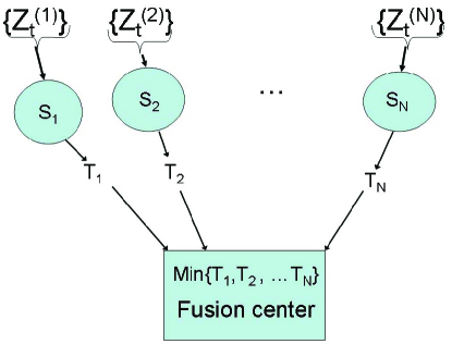
Figure 1: One shot communication in a decentralized system of $N$ sensors.

The problem of decentralized sequential detection with data fusion dates back to the 1980s with the works of [1] and [2]. We are interested in the problem of quickest detection in an $N$-sensor network in which the information available is distributed and decentralized, a problem introduced in [16]. We consider the situation in which the onset of a signal can occur at different times in the $N$ sensors, that is the change points can be different for each of the $N$ sensors. We assume that each sensor runs a cumulative sum (CUSUM) algorithm as suggested in [7, 11, 12, 13, 14] and communicates with a central fusion center only when it is ready to signal an alarm. In other words, each sensor communicates with the central fusion center through a one shot scheme. We assume that the $N$ sensors receive independent observations, which constitutes an assumption consistent with the fact that the $N$ change points can be different. So far in the literature (see [7, 11, 12, 13, 14]) it has been assumed that the change points are the same across sensors. In this paper we consider the case in which the central fusion center employs a minimal strategy, that is, it reacts when the first communication from the sensors takes place. We demonstrate that, in the situation described above, at least asymptotically, there is no loss of information at the fusion center by employing the minimal one shot scheme. That is, we demonstrate that the minimum of $N$ CUSUMs is asymptotically optimal in detecting the minimum of the $N$ different change points, as the mean time between false alarms tends to $\infty$, with respect to an appropriately extended Lorden criterion [5] that incorporates the possibility of $N$ different change points. As an observation model we consider a continuous time Brownian motion model, which is a good approximation to reality for measurements taken at a high rate. Moreover, given a high rate of observations from any distribution, the central limit theorem asserts that sums of such observations are normally distributed and therefore the Brownian motion model is a plausible model for such situations.

The communication structure considered in this paper is summarized in Figure 1, in which $T_{i}$ for $i=1,\ldots,N$ denote stopping times associated with alarms at sensors $S_{i}$ $i=1,\ldots,N$, respectively.

In the next section we formulate the problem and demonstrate asymptotic optimality (as the mean time between false alarms tends to $\infty$), in an extended min-max Lorden sense, of the minimum of $N$ CUSUM stopping times in the case of centralized detection. We then argue that this result suggests no loss in performance of the one shot minimal strategy employed by the fusion center in the case of decentralized detection. We finally discuss an extension of these results to the case of correlated sensors.

II The centralized problem

We sequentially observe the processes $\{\xi_{t}^{(i)};t\geq 0\}$ for all $i=1,\ldots,N$ with the following dynamics:

(3) $$d\xi_{t}^{(i)}=\left\{\begin{array}[]{ll}dw_{t}^{(i)}&t\leq\tau_{i}\\ \mu\,dt+dw_{t}^{(i)}&t>\tau_{i},\end{array}\right.$$

where $\mu>0$ is known , $\{w_{t}^{(i)}\}$ are independent standard Brownian motions, and the $\tau_{i}$’s are unknown constants.

An appropriate measurable space is $\Omega=C[0,\infty)\times C[0,\infty)\times\ldots\times C[0,\infty)$ and $\mathcal{F}=\cup_{t>0}\mathcal{F}_{t}$, where $\{\mathcal{F}_{t}\}$ is the filtration of the observations with $\mathcal{F}_{t}=\sigma\{s\leq t;(\xi_{s}^{(1)},\ldots,\xi_{s}^{(N)})\}$. Notice that in the case of centralized detection the filtration consists of the totality of the observations that have been received up until the specific point in time $t$.

On this space, we have the following family of probability measures $\{P_{\tau_{1},\ldots,\tau_{N}}\}$, where $P_{\tau_{1},\ldots,\tau_{N}}$ corresponds to the measure generated on $\Omega$ by the processes $(\xi_{t}^{(1)},\ldots,\xi_{t}^{(N)})$ when the change in the $N$-tuple process occurs at time point $\tau_{i}$, $i=1,\ldots,N$. Notice that the measure $P_{\infty,\ldots,\infty}$ corresponds to the measure generated on $\Omega$ by $N$ independent Brownian motions.

Our objective is to find a stopping rule $T$ that balances the trade-off between a small detection delay subject to a lower bound on the mean-time between false alarms and will ultimately detect $\min\{\tau_{1},\ldots,\tau_{N}\}$ .

As a performance measure we consider

(4) $$J_{M}^{(N)}(T)=\\ \sup_{\tau_{1},\ldots,\tau_{N}}\textrm{essup}\,E_{\tau_{1},\ldots,\tau_{N}}\left\{(T-\tau_{1}\wedge\ldots\wedge\tau_{N}\})^{+}|\mathcal{F}_{\tau_{1}\wedge\ldots\wedge\tau_{N}}\right\}$$

where the supremum over $\tau_{1},\ldots,\tau_{N}$ is taken over the set in which $\min\{\tau_{1},\ldots,\tau_{N}\}<\infty$. That is, we consider the worst detection delay over all possible realizations of paths of the $N$-tuple of stochastic processes $(\xi_{t}^{(1)},\ldots,\xi_{t}^{(N)})$ up to $\min\{\tau_{1},\ldots,\tau_{N}\}$ and then consider the worst detection delay over all possible $N$-tuples $\{\tau_{1},\ldots,\tau_{N}\}$ over a set in which at least one of them is forced to take a finite value. This is because $T$ is a stopping rule meant to detect the minimum of the $N$ change points and therefore if one of the $N$ processes undergoes a regime change, any unit of time by which $T$ delays in reacting, should be counted towards the detection delay.

The criterion presented in (4) results in the corresponding stochastic optimization problem of the form:

(5) $$\begin{array}[]{c}\displaystyle\inf_{T}J_{M}^{(N)}(T)\\ \textrm{subject to}\leavevmode\nobreak\ \leavevmode\nobreak\ \leavevmode\nobreak\ E_{\infty,\ldots,\infty}\left\{T\right\}\geq\gamma.\end{array}$$

We notice that the expectation in the above constraint is taken under the measure $P_{\infty,\ldots,\infty}$. This is the measure generated on the space $\Omega$ in the case that none of the $N$ processes $(\xi_{t}^{(1)},\ldots,\xi_{t}^{(N)})$ changes regime. Therefore, $E_{\infty,\ldots,\infty}\left\{T\right\}$ is the mean time between false alarms.

In the case of the presence of only one stochastic process (say $\{\xi_{t}^{(1)}\}$), the problem becomes one of detecting a one-sided change in a sequence of Brownian observations, or a vector of observations $(\xi_{t}^{(1)},\ldots,\xi_{t}^{(N)})$ with the same change points, whose optimal solution was found in [3] and [15]. The optimal solution is the continuous time version of Page’s CUSUM stopping rule, namely the first passage time of the process

(6) $$y_{t}^{(1)} = \sup_{0\leq\tau_{1}\leq t}\log\left.\frac{dP_{\tau_{1}}}{dP_{\infty}}\right|_{\mathcal{F}_{t}}=u_{t}^{(1)}-m_{t}^{(1)},\leavevmode\nobreak\ \textrm{where}$$

(7) $$u_{t}^{(1)} = \mu\xi_{t}^{(1)}-\frac{1}{2}\mu^{2}t,$$

and

(8) $$m_{t}^{(1)} = \inf_{0\leq s\leq t}u_{s}^{(1)}.$$

The CUSUM stopping rule is thus

(9) $$T_{\nu} = \inf\{t\geq 0;y_{t}^{(1)}\geq\nu\},$$

where $\nu$ is chosen so that $E_{\infty}\left\{T_{\nu}\right\}\equiv\frac{2}{\mu^{2}}f(\nu)=\gamma$, with $f(\nu)=e^{\nu}-\nu-1$ (see for example [4]) and

(10) $$J_{M}^{(1)}(T_{\nu})\equiv E_{0}\left\{T_{\nu}\right\}=\frac{2}{\mu^{2}}f(-\nu).$$

The fact that the worst detection delay is the same as that incurred in the case in which the change point is exactly $0$ is a consequence of the non-negativity of the CUSUM process, from which it follows that the worst detection delay occurs when the CUSUM process at the time of the change is at $0$ [4].

We remark here that if the $N$ change points were the same then the problem (5) is equivalent to observing only one stochastic process which is now $N$-dimensional. Thus, in this case, the detection delay and mean time between false alarms are given by the formulas in the above paragraph.

Returning to problem (5), it is easily seen that in seeking solutions to this problem, we can restrict our attention to stopping times that achieve the false alarm constraint with equality [8]. The optimality of the CUSUM stopping rule in the presence of only one observation process suggests that a CUSUM type of stopping rule might display similar optimality properties in the case of multiple observation processes. In particular, an intuitively appealing rule, when the detection of $\min\{\tau_{1},\ldots,\tau_{N}\}$ is of interest, is $T_{h}=T_{h}^{1}\wedge\ldots\wedge T_{h}^{N}$, where $T_{h}^{i}$ is the CUSUM stopping rule for the process $\{\xi_{t}^{(i)};t\geq 0\}$ for $i=1,\ldots,N$. That is, we use what is known as a multi-chart CUSUM stopping time [10], which can be written as

(11) $$T_{h} = \inf\left\{t\geq 0;\max\{y_{t}^{(1)},\ldots,y_{t}^{(N)}\}\geq h\right\},$$

where

$$y_{t}^{(i)}=\sup_{0\leq\tau_{i}\leq t}\left.\log\frac{dP_{\tau_{i}}}{dP_{\infty}}\right|_{\mathcal{F}_{t}}=\mu\xi_{t}^{(i)}-\frac{1}{2}\mu^{2}t-\inf_{s\leq t}\left(\mu\xi_{s}^{(i)}-\frac{1}{2}\mu^{2}s\right).$$

and the $P_{\tau_{i}}$ are the restrictions of the measure $P_{\tau_{1},\ldots,\tau_{N}}$ to $C[0,\infty)$.

It is easily seen that

$$J_{M}^{(N)}(T_{h})=E_{0,\infty,\ldots,\infty}\left\{T_{h}\right\} = E_{\infty,0,\infty,\ldots,\infty}\left\{T_{h}\right\}$$

$$= \ldots$$

$$= E_{\infty,\ldots,\infty,0}\left\{T_{h}\right\}.$$

This is because the worst detection delay occurs when at least one of the $N$ processes does not change regime. The reason for this lies in the fact that the CUSUM process is a monotone function of $\mu$, resulting in a longer on average passage time if $\mu=0$ [9]. That is, the worst detection delay will occur when none of the other processes changes regime and due to the non-negativity of the CUSUM process the worst detection delay will occur when the remaining one processes is exactly at $0$.

Notice that the threshold $h$ is used for the multi-chart CUSUM stopping rule (11) in order to distinguish it from $\nu$ the threshold used for the one sided CUSUM stopping rule (9).

In what follows we will demonstrate asymptotic optimality of (11) as $\gamma\to\infty$. In view of the discussion in the previous paragraph, in order to assess the optimality properties of the multi-chart CUSUM rule (11) we will thus need to begin by evaluating $E_{0,\infty,\ldots,\infty}\left\{T_{h}\right\}$ and $E_{\infty,\ldots,\infty}\left\{T_{h}\right\}$.

Since the processes $\xi_{t}^{(i)}$, $i=1,\ldots,N$, are independent it is possible to obtain a closed form expression through the formula

(13) $$E_{0,\infty,\ldots,\infty}\left\{T_{h}\right\}=\int_{0}^{\infty}P_{0,\infty,\ldots,\infty}(T_{h}>t)\\ =\int_{0}^{\infty}P_{0,\infty,\ldots,\infty}(\{T_{h}^{1}>t\}\cap\ldots\cap\{T_{h}^{N}>t\})dt\\ =\int_{0}^{\infty}P_{0}(T_{h}^{1}>t)\left[P_{\infty}(T_{h}^{1}>t)\right]^{N-1}dt.$$

Similarly,

(14) $$E_{\infty,\ldots,\infty}\left\{T_{h}\right\} = \int_{0}^{\infty}\left[P_{\infty}(T_{h}^{1}>t)\right]^{N}dt,$$

where $\{T_{h}^{i}>t\}=\{\sup_{0\leq s\leq t}y_{s}^{(i)}<h\}$. In other words, the evaluation of (LABEL:E0INFTY) and (14) is possible through the probability density function of the random variable $\sup_{0\leq s\leq t}y_{s}^{(i)}$ for arbitrary fixed $t$ which appears in [6].

In order to demonstrate asymptotic optimality of (11) we bound the detection delay $J_{M}^{(N)}$ of the unknown optimal stopping rule $T^{*}$ by

(15) $$E_{0,\infty,\ldots,\infty}\left\{T_{h}\right\} > J_{M}^{(N)}(T^{*}),$$

where $h$ is chosen so that

(16) $$E_{\infty,\ldots,\infty}\{T_{h}\} = \gamma.$$

It is also obvious that $J_{M}^{(N)}(T^{*})$ is bounded from below by the detection delay of the one CUSUM when there is only one observation process, in view of the fact that

$$\sup_{\tau_{1},\ldots,\tau_{N}}\textrm{essup}E_{\tau_{1},\ldots,\tau_{N}}\left\{{(T-\tau_{1}\wedge\ldots\wedge\tau_{N})}^{+}|\mathcal{F}_{\tau_{1}\wedge\ldots\wedge\tau_{N}}\right\}\geq$$

$$\geq\sup_{\tau_{1}}\textrm{essup}\,E_{\tau_{1}}\left\{{(T-\tau_{1})}^{+}|\mathcal{F}_{\tau_{1}}\right\}.$$

The stopping time that minimizes $\sup_{\tau_{1}}\textrm{essup}\,E_{\tau_{1}}\left\{{(T-\tau_{1})}^{+}|\mathcal{F}_{\tau_{1}}\right\}$ is the CUSUM stopping rule $T_{\nu}$ of (9), with $\nu$ chosen so as to satisfy

(17) $$E_{\infty}\{T_{\nu}\} = \gamma.$$

We will demonstrate that the difference between the upper and lower bounds

(18) $$E_{0,\infty,\ldots,\infty}\left\{T_{h}\right\} >J_{M}^{(N)}(T^{*}) >E_{0}\{T_{\nu}\},$$

is bounded by a constant as $\gamma\to\infty$, with $h$ and $\nu$ satisfying (16) and (17), respectively.

Lemma 1

We have

(19) $$E_{0,\infty,\ldots,\infty}\left\{T_{h}\right\} = \frac{2}{\mu^{2}}\left[\log\gamma+\log\frac{N\mu^{2}}{2}-1+o(1)\right],$$

as $\gamma\to\infty$,

Proof: Please refer to the Appendix for a sketch of the proof.

Moreover, it is easily seen from (10) that

(20) $$E_{0}\left\{T_{\nu}\right\} = \frac{2}{\mu^{2}}\left[\log\gamma+\log\frac{\mu^{2}}{2}-1+o(1)\right].$$

Thus we have the following result.

Theorem 1

The difference in detection delay $J_{M}^{(N)}$ of the unknown optimal stopping rule $T^{*}$ and the detection delay of $T_{h}$ of (11) with $h$ satisfying (16) is bounded above by

$$\frac{2}{\mu^{2}}\left(\log N\right),$$

as $\gamma\to\infty$.

Proof: The proof follows from Lemma 1 and (20).

The upper and lower bounds on detection delay for the optimal stopping rule, when $\mu$ is $\frac{1}{2}$, $1$ and $2$, in the case that $N=2$ are shown in Figure 2.

The upper and lower bounds on the detection delay (DD) for the optimal stopping rule

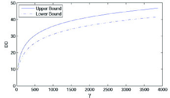
(a) $\mu=\frac{1}{2}$

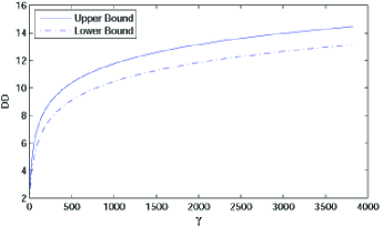
(b) $\mu=1$

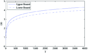
(c) $\mu=2$

Figure 2: (Left) Case of $\mu=\frac{1}{2}$. (Middle) Case of $\mu_{2}=1$. (Right) Case of $\mu=2$. (Note that the differences between upper and lowers bounds are all bounded as $\gamma$ increases.)

The consequence of Theorem 1 is the asymptotic optimality of (11) in the case in which all of the information becomes directly available through the filtration $\{\mathcal{F}_{t}\}$ at the fusion center. We notice however that this asymptotic optimality holds for any finite number of sensors $N$.

We now discuss the implications of the above result in decentralized detection in the case of one shot schemes.

III Decentralized detection

Let us now suppose that each of the observation processes $\{\xi_{t}^{(i)}\}$ become sequentially available at its corresponding sensor $S_{i}$ which then devises an asynchronous communication scheme to the central fusion center. In particular, sensor $S_{i}$ communicates to the central fusion center only when it wants to signal an alarm, which is elicited according to a CUSUM rule $T_{h}^{(i)}$ of (9). Once again the observations received at the $N$ sensors are independent and can change dynamics at distinct unknown points $\tau_{i}$. The fusion center, whose objective is to detect the first time when there is a change, devises a minimal strategy; that is, it declares that a change has occurred at the first instance when one of the sensors communicates an alarm. The implication of Theorem 1 is that in fact this strategy is the best that the fusion center can devise and that there is no loss in performance between the case in which the fusion center receives the raw data $\{\xi_{t}^{(1)},\ldots\xi_{t}^{(N)}\}$ directly and the case in which the communication that takes place is limited to the one shown in Figure 1. To see this, the detection delay of the stopping rule $T_{h}=T_{h}^{(1)}\wedge\ldots\wedge T_{h}^{(N)}$ is equal to $E_{0,\infty,\ldots,\infty}\{T_{h}\}$ when $S_{1}$ is the one that first signals an alarm, $E_{\infty,0,\ldots,\infty}\{T_{h}\}$ when $S_{2}$ first signals and so on all of which are equal due to the assumed symmetry in the signal strength $\mu$ received at each of the sensors $S_{i}$ when a change occurs. The mean time between false alarms for the fusion center that devises the rule $T_{h}=T_{h}^{(1)}\wedge\ldots\wedge T_{h}^{(N)}$ is thus $E_{\infty,\ldots,\infty}\left\{T_{h}\right\}$. But Theorem 1 asserts that this rule, namely $T_{h}$, is asymptotically optimal as the mean time between false alarms tends to $\infty$ in the centralized case for any finite $N$. In other words, the CUSUM stopping rules $T_{h}^{(1)}$, $T_{h}^{(2)}$, …, $T_{h}^{(N)}$ are sufficient statistics (at least asymptotically) for the problem of quickest detection of (5).

IV Possible extensions

An interesting extension corresponds to the case in which the signal strengths $\mu$ are different in each sensor after the change. That is, after the change the signal in $S_{i}$ is $\mu_{i}$ with $\mu_{1}\neq\mu_{2}\neq\ldots\neq\mu_{N}$. In this case, it is not clear what the optimal choice of thresholds is, but it is possible that the thresholds $\{h_{i}\}$ should be chosen so that

$$E_{0,\infty,\ldots,\infty}\{T_{C}^{N}\}=E_{\infty,0,\infty,\ldots,\infty}\{T_{C}^{N}\}=\ldots=E_{\infty,\ldots,\infty,0}\{T_{C}^{N}\},$$

where $T_{C}^{N}=T_{h_{1}}^{1}\wedge\ldots\wedge T_{h_{N}}^{N}$.

A further interesting extension corresponds to the case of correlated sensors. To demonstrate this case let us begin by assuming that $N=2$. This case corresponds to (3), but with

(21) $$E\left\{w_{t}^{(1)}w_{s}^{(2)}\right\} = \rho\min\{s,t\}\leavevmode\nobreak\ \leavevmode\nobreak\ \forall\leavevmode\nobreak\ s,t\geq 0.$$

This case becomes significantly more difficult because of the presence of local time in the dynamics of the process $\max\{y_{t}^{(1)},y_{t}^{(2)}\}$. Nevertheless, it is possible to derive a formula for the expected delay of $T_{h}$ under the measure $P_{\infty,\infty}$. This expression is given by

(22) $$E_{\infty,\infty}\left\{T_{h}\right\} = \frac{2}{\mu^{2}}(e^{h}-h-1)$$

$$- 2(1-\rho)E\left\{\int_{0}^{T}(e^{y_{t}^{(1)}}-1)\delta(y_{s}^{(1)}-y_{s}^{(2)})ds\right\},$$

where $\delta$ denotes the Dirac delta function and the final term in this expression corresponds to the collision local time of the processes $y_{t}^{(1)}$ and $y_{t}^{(2)}$ weighted by the factor $(e^{y_{t}^{(1)}}-1)$. The difficulty in the use of expression (22) is the fact that as $\rho$ changes, the expected value of the collision local time term, which is the last term in (22), also changes. Moreover, the expression for the first moment of $T_{h}$ becomes significantly more complicated under the measure $P_{0,\infty}$.

V Appendix

As an illustration for general case, let us prove the result for $N=2$.

We begin by deriving expressions for $E_{0,\infty}\left\{T_{h}\right\}$ and $E_{\infty,\infty}\left\{T_{h}\right\}$ by using the results in [6]. For all $h>2$, we have

$$E_{0,\infty}\left\{T_{h}\right\}=\\ \frac{32}{\mu^{2}}\sum_{i,j\geq 1}\frac{\sin^{3}\phi_{i}\sin^{3}\theta_{j}}{(\phi_{i}-\sin\phi_{i}\cos\phi_{i})(\theta_{j}-\sin\theta_{j}\cos\theta_{j})}\frac{\cos^{2}\phi_{i}\cos^{2}\theta_{j}}{\cos^{2}\phi_{i}+\cos^{2}\theta_{j}}\\ -\frac{32}{\mu^{2}}\frac{\sinh^{3}\eta}{\sinh\eta\cosh\eta-\eta}\sum_{i\geq 1}\frac{\sin^{3}\phi_{i}\cos^{2}\phi_{i}}{\phi_{i}-\sin\phi_{i}\cos\phi_{i}}\frac{\cos^{2}\phi_{i}}{\cos^{2}\phi_{i}+\cosh^{2}\eta}\\ +\frac{32}{\mu^{2}}\frac{\sinh^{3}\eta}{\sinh\eta\cosh\eta-\eta}\sum_{i\geq 1}\frac{\sin^{3}\phi_{i}\cos^{2}\phi_{i}}{\phi_{i}-\sin\phi_{i}\cos\phi_{i}}\\ =S_{1}(h)+S_{2}(h)+S_{3}(h),$$

and

$$E_{\infty,\infty}\left\{T_{h}\right\}=\\ \frac{32}{\mu^{2}}\sum_{i,j\geq 1}\frac{e^{-h}\sin^{3}\theta_{i}\sin^{3}\theta_{j}}{(\theta_{i}-\sin\theta_{i}\cos\theta_{i})(\theta_{j}-\sin\theta_{j}\cos\theta_{j})}\frac{\cos^{2}\theta_{i}\cos^{2}\theta_{j}}{\cos^{2}\theta_{i}+\cos^{2}\theta_{j}}\\ +\frac{64}{\mu^{2}}\frac{e^{-h}\sinh^{3}\eta}{\sinh\eta\cosh\eta-\eta}\sum_{i\geq 1}\frac{\sin^{3}\theta_{i}\cos^{2}\theta_{i}}{\theta_{i}-\sin\theta_{i}\cos\theta_{i}}\frac{\cosh^{2}\eta}{\cos^{2}\theta_{i}+\cosh^{2}\eta}\\ +\frac{16}{\mu^{2}}\frac{e^{-h}\sinh^{6}\eta\cosh^{2}\eta}{(\sinh\eta\cosh\eta-\eta)^{2}}\\ =S_{4}(h)+S_{5}(h)+S_{6}(h),$$

where

$$\tan\phi_{n} = -\frac{2}{h}\phi_{n}<0$$

$$\tan\theta_{n} = \frac{2}{h}\theta_{n}>0$$

$$\tanh\eta = \frac{2}{h}\eta>0.$$

The idea then is show $S_{1}(h)$, $S_{2}(h)$, $S_{4}(h)$ and $S_{5}(h)$ converge to zero, and examine how $S_{2}(h)$ and $S_{5}(h)$ behave as $h\to\infty$. In the following paragraphs we shall analyze these in the order $S_{6}(h)\rightarrow S_{3}(h)\rightarrow S_{2}(h)\rightarrow S_{5}(h)\rightarrow S_{1}(h)\rightarrow S_{4}(h)$.

First notice that for large $h$, $\eta$ is large and close to $\frac{h}{2}$. Moreover,

(23) $$e^{2\eta-h}=1-4\eta e^{-2\eta}+o(e^{-3\eta}).$$

This can help us to compare $\eta$ with $h$.

For $S_{6}(h)$,

$$S_{6}(h) = \frac{16}{\mu^{2}}e^{-h}\sinh^{4}\eta\left(1-\eta\sinh^{-1}\eta\cosh^{-1}\eta\right)^{-2}$$

$$= \frac{1}{\mu^{2}}e^{-h}\left[e^{4\eta}+\left(8\eta-4\right)e^{2\eta}+o(e^{\eta})\right]$$

$$= \frac{1}{\mu^{2}}\left[e^{h}e^{4\eta-2h}+(8\eta-4)e^{2\eta-h}+o(e^{-\eta})\right],$$

by (23) the first term is

$$e^{h}e^{4\eta-2h} = e^{h}\left(e^{2\eta-h}\right)^{2}=e^{h}\left[1-4\eta e^{-2\eta}+o(e^{-3\eta})\right]^{2}$$

$$= e^{h}\left[1-8\eta e^{-2\eta}+o(e^{-3\eta})\right]$$

$$= e^{h}-8\eta e^{h-2\eta}+o(e^{-\eta})$$

$$= e^{h}-8\eta+o(e^{-\eta}),$$

and the second term is

$$(8\eta-4)e^{2\eta-h} = (8\eta-4)\left[1+o(e^{-\eta})\right]$$

$$= 8\eta-4+o(e^{-\eta}),$$

so

(24) $$S_{6}(h) = \frac{1}{\mu^{2}}\left[e^{h}-4+o(e^{-\frac{h}{2}})\right],\leavevmode\nobreak\ \textrm{as}\leavevmode\nobreak\ h\to\infty.$$

For $S_{3}(h)$, also note that from (10) and [6] we can write

(25) $$\frac{2}{\mu^{2}}f(-h) = \int_{0}^{\infty}P_{0}(T_{h}>t)dt$$

$$= \frac{16}{\mu^{2}}e^{\frac{h}{2}}\sum_{i\geq 1}\frac{\sin^{3}\phi_{i}\cos^{2}\phi_{i}}{\phi_{i}-\sin\phi_{i}\cos\phi_{i}},$$

from which we obtain

(26) $$S_{3}(h) = \frac{32}{\mu^{2}}\frac{\sinh^{3}\eta}{\sinh\eta\cosh\eta-\eta}\sum_{i\geq 1}\frac{\sin^{3}\phi_{i}\cos^{2}\phi_{i}}{\phi_{i}-\sin\phi_{i}\cos\phi_{i}}$$

$$= \frac{2}{\mu^{2}}\left[1+o(e^{-\eta})\right](h+e^{-h}-1)$$

$$= \frac{2}{\mu^{2}}\left[h-1+o(e^{-\frac{h}{2}})\right],\leavevmode\nobreak\ \textrm{as}\leavevmode\nobreak\ h\to\infty.$$

To bound $S_{2}(h)$ and $S_{5}(h)$ we need the following,

Result 1: Suppose $0<p<1$. Then, for all positive solutions $\{\alpha_{i}\}_{i\geq 1}$ to the equation $\tan x=px$ ($\tan x=-px$, resp.), we have

(27) $$\lim_{p\to 0^{+}}\sum_{i\geq 1}\frac{|\sin^{3}\alpha_{i}|\cos^{2}\alpha_{i}}{\alpha_{i}-\sin\alpha_{i}\cos\alpha_{i}}\leq\frac{1}{\pi}.$$

This suggests that, asymptotically, as $h\to\infty$,

$$\frac{\sinh^{3}\eta}{\sinh\eta\cosh\eta-\eta}\sum_{i\geq 1}\frac{|\sin^{3}\phi_{i}|\cos^{2}\phi_{i}}{\phi_{i}-\sin\phi_{i}\cos\phi_{i}}\frac{\cos^{2}\phi_{i}}{\cos^{2}\phi_{i}+\cosh^{2}\eta}\\ \leq\left[\frac{1}{\pi}+o(1)\right]\frac{\sinh^{3}\eta}{\cosh^{2}\eta(\sinh\eta\cosh\eta-\eta)}\\ =\left[\frac{1}{\pi}+o(1)\right]\frac{\sinh^{2}\eta}{\cosh^{3}\eta}\left(1-\eta\sinh^{-1}\eta\cosh^{-1}\eta\right)^{-1}\\ =O(e^{-\frac{h}{2}}),$$

from which we obtain

(28) $$|S_{2}(h)| = \frac{2}{\mu^{2}}O(e^{-\frac{h}{2}}),\leavevmode\nobreak\ \textrm{as}\leavevmode\nobreak\ h\to\infty.$$

Similarly,

$$\frac{e^{-h}\sinh^{3}\eta}{\sinh\eta\cosh\eta-\eta}\sum_{i\geq 1}\frac{|\sin^{3}\theta_{i}|\cos^{2}\theta_{i}}{\theta_{i}-\sin\theta_{i}\cos\theta_{i}}\frac{\cosh^{2}\eta}{\cos^{2}\theta_{i}+\cosh^{2}\eta}\\ \leq\left[\frac{1}{\pi}+o(1)\right]e^{-h}\frac{\sinh^{2}\eta}{\cosh\eta}\left(1-\eta\sinh\eta\cosh\eta\right)^{-1}\\ =O(e^{-\frac{h}{2}}),$$

so

(29) $$|S_{5}(h)| = \frac{1}{\mu^{2}}O(e^{-\frac{h}{2}}),\leavevmode\nobreak\ \textrm{as}\leavevmode\nobreak\ h\to\infty.$$

To handle the double sum in $S_{1}(h)$ and $S_{4}(h)$, we need

Result 2: Suppose $0<p<1$, $\{\alpha_{i}\}_{i\geq 1}$ are all positive solutions to the equation $\tan x=px$, and $\{\beta_{i}\}_{i\geq 1}$ are all positive solutions to equation $\tan x=px$ ($\tan x=-px$, resp.), then

$$\sum_{i,j\geq 1}\frac{\sin^{3}\alpha_{i}\sin^{3}\beta_{j}}{(\alpha_{i}-\sin\alpha_{i}\cos\alpha_{i})(\beta_{j}-\sin\beta_{j}\cos\beta_{j})}\frac{\cos^{2}\alpha_{i}\cos^{2}\beta_{j}}{\cos^{2}\alpha_{i}+\cos^{2}\beta_{j}}$$

(30) $$\to 0,\leavevmode\nobreak\ \textrm{as}\leavevmode\nobreak\ p\to 0^{+}.$$

Consequently,

(31) $$|S_{1}(h)| = o(1),\leavevmode\nobreak\ \textrm{as}\leavevmode\nobreak\ h\to\infty.$$

Similarly,

(32) $$|S_{4}(h)| = \frac{1}{\mu^{2}}o(e^{-h}),\leavevmode\nobreak\ \textrm{as}\leavevmode\nobreak\ h\to\infty.$$

Finally, from (24), (26), (28), (29), (31) and (32) we obtain

(33) $$\hskip 12.91663ptE_{0,\infty}(T_{h}) = \frac{2}{\mu^{2}}\left[h-1+o(1)\right],\leavevmode\nobreak\ \textrm{as}\leavevmode\nobreak\ h\to\infty,$$

and

(34) $$E_{\infty,\infty}(T_{h}) = \frac{1}{\mu^{2}}\left[e^{h}-4+o(1)\right],\leavevmode\nobreak\ \textrm{as}\leavevmode\nobreak\ h\to\infty.$$

And for $h$ and $\gamma$ satisfying (16), we have asymptotic results (19) with $N=2$.

Now let us prove the two results we used in the above.
Result 1:

Proof:

For any $\alpha_{i}\in\left((i-\frac{1}{2})\pi,(i+\frac{1}{2})\pi\right)$ such that $\tan\alpha_{i}=\pm p\alpha_{i}$, ($0<p<1$), we have

$$\frac{|\sin^{3}\alpha_{i}|\cos^{2}\alpha_{i}}{\alpha_{i}-\sin\alpha_{i}\cos\alpha_{i}}=\frac{p^{3}\alpha_{i}^{2}}{(1+p^{2}\alpha_{i}^{2})^{3/2}\left[(1\mp p)+p^{2}\alpha_{i}^{2}\right]}\\ \leq\frac{p}{(1+p^{2}\alpha_{i}^{2})^{3/2}}\leq\frac{p}{\left[1+p^{2}\left(i-\frac{1}{2}\right)^{2}\pi^{2}\right]^{3/2}}.$$

Thus

$$\sum_{i\geq 1}\frac{|\sin^{3}\alpha_{i}|\cos^{2}\alpha_{i}}{\alpha_{i}-\sin\alpha_{i}\cos\alpha_{i}}\leq\sum_{i\geq 1}\frac{p}{\left[1+p^{2}\left(i-\frac{1}{2}\right)^{2}\pi^{2}\right]^{3/2}}\\ \leq\frac{1}{\pi}\int_{-\frac{\pi}{2}}^{\infty}\frac{pdx}{(1+p^{2}x^{2})^{3/2}}=\frac{1}{\pi}\int_{-p\frac{\pi}{2}}^{\infty}\frac{du}{(1+u^{2})^{3/2}}\\ \to\int_{0}^{\infty}\frac{du}{(1+u^{2})^{3/2}}=\frac{1}{\pi},\leavevmode\nobreak\ \textrm{as}\leavevmode\nobreak\ p\to 0^{+}.$$

∎

Result 2:

Proof:

For simplicity let us denote the $(i,j)$-term in the sum by $a_{i,j}(p)$. As in the last proof, a little computation would give us

$$|a_{i,j}(p)| = I_{p}(p\alpha_{i},p\beta_{j})\cdot p^{2},$$

where $I_{p}(x,y)$ $(0<p<1)$ is the function

$$I_{p}(x,y)=\\ \frac{1}{\sqrt{(1+x^{2})(1+y^{2})}(2+x^{2}+y^{2})(1+\frac{1-p}{x^{2}})(1+\frac{1\mp p}{y^{2}})}.$$

Clearly, $I_{p}(\cdot,\cdot)$ is (uniformly in $p$, $0\leq p<1$) bounded above by the $L^{1}(\mathbb{R}^{2})$ function $B(\cdot,\cdot)$, which is defined as

$$B(x,y) = \frac{1}{\sqrt{(1+x^{2})(1+y^{2})}(2+x^{2}+y^{2})}.$$

We have two steps to finish our proof:

$$(a)\lim_{p\to 0^{+}}\sum_{i,j\geq 1}|a_{i,j}(p)|=\frac{1}{\pi^{2}}\int\int_{(\mathbb{R}^{+})^{2}}I_{0}(x,y)dxdy,$$

$$(b)\lim_{p\to 0^{+}}\sum_{i,j\geq 1}a_{i,j}(p)\cdot\mathbb{I}_{\{a_{i,j}(p)>0\}}\\ =\frac{1}{2\pi^{2}}\int\int_{(\mathbb{R}^{+})^{2}}I_{0}(x,y)dxdy.$$

Let us start from (a). Given any $\epsilon>0$, we can find a constant $M>0$ such that, for $R_{M}=\{(x,y):\min(x,y)>M\}$ and all $0\leq p<1$,

$$\begin{cases}&I_{p}\leavevmode\nobreak\ \textrm{is decreasing in both}\leavevmode\nobreak\ x\leavevmode\nobreak\ \textrm{and}\leavevmode\nobreak\ y\leavevmode\nobreak\ \textrm{in}\leavevmode\nobreak\ R_{M},\\ &\frac{1}{\pi^{2}}\int\int_{R_{M}}I_{p}(x,y)dxdy\leq\frac{1}{\pi^{2}}\int\int_{R_{M}}B(x,y)dxdy\leq\frac{\epsilon}{3}.\end{cases}$$

Because of this, for any $0\leq p<1$, the “tail” sum

$$\sum_{\min(p\alpha_{i},p\beta_{j})>M+p\pi}|a_{i,j}(p)|\leq\frac{1}{\pi^{2}}\int\int_{R_{M}}I_{p}(x,y)dxdy\leq\frac{\epsilon}{3},$$

where we define $a_{i,j}(0)=0$ for all $(i,j)$.

(38) $$\sum_{i,j\geq 1}\frac{\sin^{3}\phi_{i}\sin^{3}\theta_{j}\cos^{2}\phi_{i}\cos^{2}\theta_{j}}{(\phi_{i}-\sin\phi_{i}\cos\phi_{i})(\theta_{j}-\sin\theta_{j}\cos\theta_{j})[(N-2)(1-4\frac{\eta^{2}}{h^{2}})\cos^{2}\phi_{i}\cos^{2}\theta_{j}+\cos^{2}\phi_{i}+\cos^{2}\theta_{j}]}\\$$

(39) $$I_{p}^{(N)}(x,y)=\frac{1}{\sqrt{(1+x^{2})(1+y^{2})}[(N-2)(1-p^{2}\eta^{2})+2+x^{2}+y^{2}](1+\frac{1-p}{x^{2}})(1+\frac{1+p}{y^{2}})}$$

On the other hand, as $p$ goes to zero, the function $I_{p}$ will converge uniformly in $[0,M]^{2}$ to $I_{0}$. So all the terms $|a_{i,j}(p)|$ in the “head” sum are uniformly very close to $I_{0}(p\alpha_{i},p\beta_{j})\cdot p^{2}$, the sum of which, multiplied by $\pi^{2}$, is a Riemann sum of the function $I_{0}(x,y)$ over the region $[0,M]^{2}$, and will converges to the Riemann integral of $I_{0}$ over $[0,M]^{2}$ as $p$ turns to zero. In other words, for small $p$, there exists

$$\left|\sum_{\max(p\alpha_{i},p\beta_{j})\leq M+p\pi}|a_{i,j}(p)|-\frac{1}{\pi^{2}}\int_{0}^{M}\int_{0}^{M}I_{0}(x,y)dxdy\right|$$

(36) $$\leq\frac{\epsilon}{3}.$$

By (V) and (V), we have

$$\left|\lim_{p\to 0^{+}}\sum_{i,j\geq 1}|a_{i,j}(p)|-\frac{1}{\pi^{2}}\int\int_{(\mathbb{R}^{+})^{2}}I_{0}(x,y)dxdy\right|\leq\epsilon.$$

Now let $\epsilon$ goes to zero we are done with (a).

The proof of (b) is similar. Note that the signs of the $a_{i,j}(p)$’s can be represented by $(-1)^{i+j}$ or $(-1)^{i+j+1}$, and in each rectangle $[2(i-1)p\pi,2ip\pi]\times[(j-1)p\pi,jp\pi],(i,j\geq 1)$, either $a_{2i-1,j}(p)$ or $a_{2i,j}(p)$ is positive. With the same constant $M$ chosen as above, for the sum of all positive $a_{i,j}(p)$’s such that $\max(p\alpha_{i},p\beta_{j})\leq M+p\pi$, we can use the same argument as before, to show that for small $p$,

$$2\pi^{2}\left(\sum_{\max(p\alpha_{i},p\beta_{j})\leq M+p\pi}a_{i,j}(p)\cdot\mathbb{I}_{\{a_{i,j}(p)>0\}}\right)$$

(38) $$\approx\int_{0}^{M}\int_{0}^{M}I_{0}(x,y)dxdy.$$

Thus (b) is proven because both the tail integral and the tail sum are negligible due the way to choose $M$. ∎

In the $N$ CUSUMs case with $N\geq 2$, the calculation is similar: both of the main terms in $E_{0,\infty,\ldots,\infty}\left\{T_{h}\right\}$ and in $E_{\infty,\infty,\ldots,\infty}\left\{T_{h}\right\}$ are the terms with highest degree in $\left[\sinh^{3}\eta/(\sinh\eta\cosh\eta-\eta)\right]$. With (23) we can get they are

(39) $$\frac{2}{\mu^{2}}[h-1+o(e^{-\frac{h}{2}})],$$

and

(40) $$\frac{2}{N\mu^{2}}\left[e^{h}+(N-2)h+(2-3N)+o(e^{-\frac{h}{2}})\right],$$

respectively.

We can prove that all other terms converge to zero as $h$ goes to infinity.

With a generalization of Result 1 to $n$ dimensional trigonometric sums and integrals for all $n\geq 1$, we are able to deal with most terms in the expansion of the expectations, because those bounded trigonometric sums are multiplied by expressions of negative exponential order in $h$.

There is only one term (in $E_{0,\infty,\ldots,\infty}\left\{T_{h}\right\}$) which cannot be proven to converge to zero in this manner. We need to prove the sum involved there, which is (38) at the top of the following page, converges to zero as $h$ goes to infinity. We can follow the proof of Result 2 to get the result. To be more precise, denote $p=\frac{2}{h}$, and the term in above sum by $a_{i,j}^{(N)}(p)$, then obviously, $|a_{i,j}^{(N)}(p)|\leq|a_{i,j}^{(2)}(p)|$, that can help us to control the “tail” sum

(40) $$\sum_{\min(p\phi_{i},p\theta_{j})>M+p\pi}|a_{i,j}^{(N)}(p)|,$$

where $M$ is chosen as in the proof of Result 2. On the other hand,

(41) $$|a_{i,j}^{(N)}(p)|=I_{p}^{(N)}(p\phi_{i},p\theta_{j})\cdot p^{2},$$

where $I_{p}^{(N)}$ is the function defined in (39). The function $I_{p}^{(N)}$ uniformly converges to $I_{0}$ as $p$ goes to infinity in the domain $[0,M]^{2}$, since $p\eta\to 1$ as $p\to 0^{+}$. As a result, the “head” sum converges to the same double integral as the one in (V) or (V), so we are done!

Finally, by (39) and (40), we can derive asymptotic formula (19) with $h$ and $\gamma$ satisfying (16).

References

[1]
M. M. Al-Ibrahim and P. K. Varshney, A simple multi-sensor sequential detection
procedure, Proceedings of the 27th IEEE Conference on Decision and Control,
Austin, Texas, pp. 2479-2483, Deecember 1988.
[2]
M. M. Al-Ibrahim and P. K. Varshney, A decentralized sequential test with data
fusion, Proceedings of the 1989 American Control Conference, Pittsburgh,
Pennsylvania, pp. 1321-1325, June 1989.
[3]
M. Beibel, A note on Ritov’s Bayes approach to the minimax property of the CUSUM
procedure, Annals of Statistics, Vol. 24, No. 2, pp. 1804 - 1812, 1996.
[4]
O. Hadjiliadis and G. V. Moustakides, Optimal and asymptotically optimal CUSUM rules
for change point detection in the Brownian motion model with multiple alternatives,
Theory of Probability and Its Applications, Vol. 50, No. 1, pp. 131 - 144,
2006.
[5]
G. Lorden, Procedures for reacting to a change in distribution, Annals of
Mathematical Statistics, Vol. 42, No. 6, pp. 1897 - 1908, 1971.
[6]
M. Magdon-Ismail, A.F. Atiya, A. Pratap and Y.S. Abu-Mostafa, On the maximum
drawdown of Brownian motion, Journal of Applied Probability, Vol. 41, No. 1,
pp. 147–161.
[7]
G. V. Moustakides, Decentralized CUSUM change detection, Proceedings of the 9th
International Conference on Information Fusion (ICIF), Florence, Italy, pp. 1 - 6,
2006.
[8]
G. V. Moustakides, Optimal stopping times for detecting changes in distributions,
Annals of Statistics, Vol. 14, No. 4, pp. 1379 - 1387, 1986.
[9]
H.V. Poor and O. Hadjiliadis, Quickest Detection, Cambridge University Press,
Cambridge UK (to appear).
[10]
A. G. Tartakovsky, Asymptotic performance of a multichart CUSUM test under false
alarm probability constraint, Proceedings of the 44th IEEE Conference on
Decision and Control, Seville, Spain, December 12 - 15 2005, pp. 320 - 325.
[11]
A.G. Tartakovsky and H. Kim, Performance of certain decentralized distributed change
detection procedures, Proceedings of the 9th International Conference on
Information Fusion, Florence, Italy, July 8-10 2006.
[12]
A.G. Tartakovsky and V. V. Veeravalli, Quickest change detection in distributed
sensor systems, Proceedings of the 6th Conference on Information Fusion,
Cairns, Australia, July 8-11 2003.
[13]
A.G. Tartakovsky and V. V. Veeravalli, Change-point detection in multichannel and
distributed systems with applications, in Applications of Sequential
Methodologies, pp. 331-363, (N. Mukhopadhay, S.Datta and S. Chattopadhay, Eds),
Marcel Dekker, New York, 2004.
[14]
A.G. Tartakovsky and V. V. Veeravalli, Asymptotically optimum quickest change
detection in distributed sensor systems, Sequential Analysis, to appear.
[15]
A. N. Shiryaev, Minimax optimality of the method of cumulative sums (cusum) in the
continuous case, Russian Mathematical Surveys, Vol. 51, No. 4, pp. 750 - 751,
1996.
[16]
V. V. Veeravalli, Decentralized quickest change detection, IEEE Transactions on
Information Theory, Vol. 47, No. 4, pp. 1657 - 1665, 2001.