GLAS-PPE/2008-0924${}^{\underline{\rm{th}}}$ July 2008

This note validates the usage of the simplified detector geometry description. A sample of $B^{0}_{(s)}\to h^{+}h^{{}^{\prime}-}$ decays was used to assess the tracking and physics performance with respect to what is obtained with the full detector description. No significant degradation of performance was found.

LHCb Public Note, LHCb-2008-030

1 Introduction

The reconstruction of tracks is an important but time-consuming task. It is well known that track fitting contributes substantially to the reconstruction time budget. Detailed studies show that a large fraction of the time spent in fitting tracks is due to the many calculations of material intersections along a particle’s path. These are necessary in order to account for the detector material by means of multiple scattering and energy loss corrections.

A simplified description of the detector material as seen by a particle traversing the LHCb detector has recently been implemented [1]. It replaces the full detector material description by a small set of simple modules (mostly boxes and cylinders) that model the average material properties.

In this note we study the implications of using this simplified geometry when accounting for detector material during track fitting. We compare the performance of the simplified versus the full geometry with a sample of $B^{0}\to\pi^{+}\pi^{-}$ events in terms of track fit quality, quality of reconstruction and event selection, and physics analysis. Note that all results are obtained starting from the same data sample generated and simulated with the full geometry in Geant4.

2 Pattern recognition

LHCb pattern recognition algorithms ignore any material effects and should therefore be insensitive to whether the simplified geometry description is used (an exception is explained below). Those considered in this note are:

• finding of tracks in the vertex locator (VELO) in $r$-$z$ and 3D-space. The algorithms are hereafter denoted by VeloR and VeloSpace, respectively [2];

• finding of tracks that traverse the whole LHCb detector (called “long tracks”). The two existing long tracking algorithms are hereafter denoted Forward [3] and Matching [4].

In Table 1 the efficiencies  for the VeloR, VeloSpace, Forward, and Matching pattern recognition algorithms are compared. All efficiencies are quoted for long tracks with no momentum cut applied. As expected, all efficiencies are identical, with the exception of the Matching efficiency, whose difference can be understood as the algorithm matches T-station seed tracks to VELO track segments by extrapolating them to the magnet region, and the extrapolation internally looks at the material along the track’s trajectory.

An identical conclusion can be drawn for the number of clone tracks and the ghost rate of all four algorithms.

	VeloR	VeloSpace	Forward	Matching
Geometry	efficiency (%)	efficiency (%)	efficiency (%)	efficiency (%)
full	$98.0\pm 0.1$	$97.0\pm 0.1$	$85.9\pm 0.2$	$81.1\pm 0.2$
simplified	$98.0\pm 0.1$	$97.0\pm 0.1$	$85.9\pm 0.2$	$81.4\pm 0.2$

Table 1: VeloR, VeloSpace, Forward and Matching pattern recognition efficiencies for the full and the simplified geometries.

For completeness the tracks pseudorapidity, $\eta$, distributions as obtained with the Forward and the Matching pattern recognition algorithms are compared in Figure 1. No significant differences are observed, as expected, even in the very forward $\eta$ region where effects of the simplified description are most likely to be evident as high-$\eta$ tracks traverse more material.

Figure 1: Distributions in tracks pseudorapidity as obtained with the (a) Forward and the (b) Matching pattern recognition algorithms for the full and the simplified geometries.

3 Track fitting

Pattern recognition tracks are fitted in order to obtain the best estimate of the track parameter values and errors. During the fitting procedure some of the hits on the tracks (called LHCbIDs) are flagged as outliers and removed from the tracks. The distributions of outliers removed by the fitter for Forward and Matching tracks are compared in Figure 2. Irrespective of the geometry used, Forward tracks tend to have more outliers than Matching tracks. When using the simplified geometry, this tendency is less pronounced. In particular, Matching tracks fitted with the simplified geometry lose slightly more hits compared to when they are fitted with the full geometry.

Figure 2: Distributions of outlier hits as obtained with the (a) Forward and the (b) Matching pattern recognition algorithms for the full and the simplified geometries.

Figure 3: Resolutions on the track parameters at the first measurement point for the full and the simplified geometries. This sample of long tracks was obtained with the Forward pattern recognition algorithm.

Figure 4: Pull distributions of the track parameters at the first measurement point for the full and the simplified geometries. This sample of long tracks was obtained with the Forward pattern recognition algorithm.

Figure 5: Resolutions on the track parameters in the Outer Tracker region for the full and the simplified geometries. This sample of long tracks was obtained with the Forward pattern recognition algorithm.

Figure 6: Resolutions in (a) momentum versus pseudorapidity, in (b) pseudorapidity versus pseudorapidity and in (c) momentum versus momentum, as given by the $\sigma$ values of single-Gaussian fits. Figure (d) shows the result of a single-Gaussian fit to the momentum resolution averaged over the momentum range in (c). All the distributions were obtained for the full and the simplified geometries with the Forward pattern recognition algorithm.

The quality of track fitting is straightforwardly assessed looking at the resolutions and the pull distributions of the track state parameters: positions $x$ and $y$, slopes $t_{x}$ and $t_{y}$, and charge-over-momentum ratio $q/p$.

All the distributions shown in this section were obtained with the Forward algorithm. However, it has been checked that all the following conclusions also hold for long tracks from the Matching algorithm.

The track parameter resolutions at the first track measurement point – quantities dominated by the VELO measurements – are collected in Figure 3. Neither the position nor the slope resolutions deteriorate when using the simplified rather than the full geometry. A slight increase in the momentum resolution (here taken as the root mean squared, RMS, rather than the $\sigma$ of a single-Gaussian fit) from $0.60\%$ to $0.63\%$ is observed. The increase originates mostly from a broadening in the left part of the distribution, where $p_{rec}<p_{true}$.

Figure 4 shows the pull distributions at the first track measurement point. No differences are observed between the full and the simplified geometries apart from a slight increase in the momentum bias; it increases from $0.05\pm 0.006$ to $0.12\pm 0.006$.

The exercise was repeated at different locations along the track’s trajectory: resolutions and pull distributions were calculated at the track’s origin vertex position and at positions in the various tracking detectors. One such example of resolution distributions in the region of the Outer Tracker is presented in Figure 5. In all cases the same conclusions can be drawn as for the distributions at the first measurement point.

The momentum resolution was also studied as a function of the momentum and the pseudorapidity of the tracks. The distributions collected in Figure 6 profile the $\sigma$ values of single-Gaussian fits to the momentum resolution. A small deterioration can be observed over the full momentum and $\eta$ spectra.

The momentum resolution versus momentum was projected onto the $y$-axis to obtain an average resolution over (most of) the spectrum; the results of single-Gaussian fits to the obtained projection distributions (Figure 6(d)) show a core momentum resolution of $0.44\%$ and $0.45\%$ with the full and the simplified geometry, respectively.

Figure 6(b) further shows the tracks pseudoradipity resolution as a function of pseudorapidity. No degradation of resolution was observed.

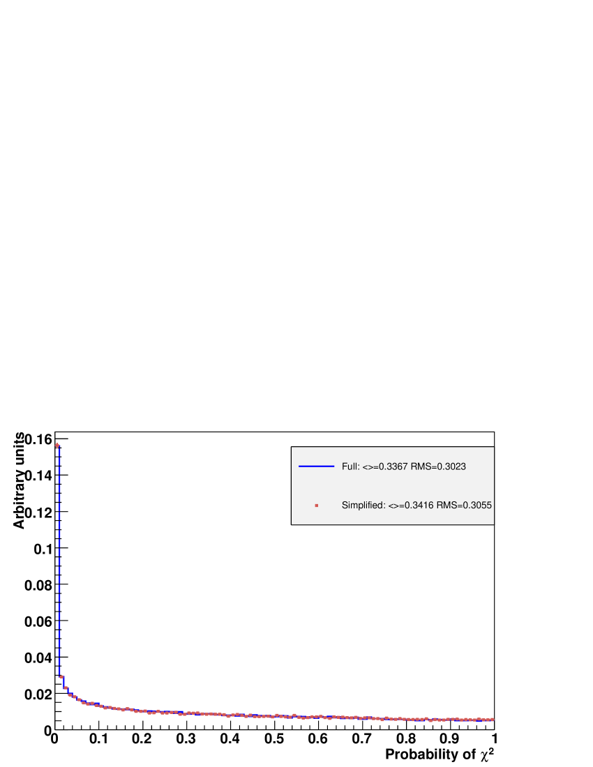
Figure 7: Track fit probability of $\chi^{2}$ distribution for long tracks found by the Forward pattern recognition algorithm for the full and the simplified geometries.

The probability of track fit $\chi^{2}$ is another measure of the fit quality; an accurate fit model should give rise to a flat distribution (a discussion can be found in [5]). Figure 7 compares the $\chi^{2}$ probability distribution obtained with the full and the simplified geometries. Both distributions agree very well.

4 Physics analysis

In this section the impact of using the simplified geometry for track fitting on the quality of the selection and reconstruction of B decays is studied. The $B^{0}\to\pi^{+}\pi^{-}$ decay (extensively described in [6]) was used for the sake of example.

4.1 Effect on the event selection

B decays are typically selected exploiting the high mass and long lifetime of B mesons. The discriminating variables used are the transverse momentum and impact parameter of the B and its daughters and the flight-distance of the B. In Table 2 the selection cuts applied to the generic $B^{0}_{(s)}\to h^{+}h^{{}^{\prime}-}$ channels are shown (a more detailed explanation of all cuts can be found in [6]).

$B^{0}_{(s)}\to h^{+}h^{{}^{\prime}-}$ selection parameter	cut value
smallest $p_{t}$($\mathrm{GeV}$) of the daughters	$>$ 1.0
largest $p_{t}$($\mathrm{GeV}$) of the daughters	$>$ 3.0
$B^{0}_{(s)}$ $p_{t}$($\mathrm{GeV}$)	$>$ 1.2
smallest $IP/\sigma_{IP}$ of the daughters	$>$ 6
largest $IP/\sigma_{IP}$ of the daughters	$>$ 12
$B^{0}_{(s)}$ $IP/\sigma_{IP}$	$<$ 2.5
$B^{0}_{(s)}$ vertex fit $\chi^{2}$	$<$ 5
($L$)$/\sigma_{L}$	$>$ 18
$|\Delta$m$|$($\mathrm{MeV}$)	$<$ 50

Table 2: Selection cuts applied to the $B^{0}_{(s)}\to h^{+}h^{{}^{\prime}-}$ channels [6].

The distributions of the various $B^{0}_{(s)}\to h^{+}h^{{}^{\prime}-}$ selection variables are shown in Figures 8 to 10. Positively and negatively charged pions were looked at independently to track down any possible charge-induced biases. Note that all plots were obtained after applying the full selection on all the variables but the plotted one. In case of the $p_{T}$ and impact parameter significance cuts on the pions, where one threshold is applied to both pions and another has to be exceeded by at least one of them, these cuts have been switched off simultaneously. In addition, normalised integrals are shown to give a direct comparison of the acceptances obtained with the full and the simplified setups. The distributions obtained with the simplified geometry agree very well with those obtained with the full setup. The observed differences were at most at the percent level.

Figure 8: Distributions of the event selection variables of impact parameter significances for (a) the $B^{0}$ candidate and its daughter (c) positively and (e) negatively charged pions for the full and simplified geometries (full and dashed lines, respectively). The right-hand-side distributions correspond to the integrated left-hand-side distributions.

Figure 9: Distributions of the event selection variables of (a) $B^{0}$ and daughter (c) positively and (e) negatively charged pions transverse momentum for the full and simplified geometries (full and dashed lines, respectively). The right-hand-side distributions correspond to the integrated left-hand-side distributions.

Figure 10: Distributions of $B^{0}$ (a) decay vertex $\chi^{2}$, (c) flight distance significance and (e) invariant mass for the full and simplified geometries (full and dashed lines, respectively). The right-hand-side distributions correspond to the integrated left-hand-side distributions.

As the differences in the single-cut variables partly cancel out, the overall change in the number of selected $B^{0}_{(s)}\to h^{+}h^{{}^{\prime}-}$ events is $\approx$1% (Table 3). Still, as can be seen from the table, the percentage of common events selected with the full and the simplified geometries is $\approx$95-96%, whereas $\approx$4-5% of the events in each sample are only present in that particular sample. In the following all comparison distributions were obtained with all the selected events, i.e. using both common and non-common events.

	Number of selected	Events only	In common
Geometry	events	in the sample	with other sample
full	4141	162 (3.9%)	3979 (96.1%)
simplified	4186	207 (4.9%)	3979 (95.1%)

Table 3: Number of selected events after running the $B^{0}_{(s)}\to h^{+}h^{{}^{\prime}-}$ selection for the full and the simplified geometries. The third and the forth rows indicate, respectively, the number (and percentage) of selected events only present in the “full” and in the “simplified” samples and the number of events in common.

4.2 Effect on resolutions

Finally, the resolution on the most important physics analysis observables were compared: momentum resolutions have been studied as well as the resolutions on the primary and secondary ($B^{0}$ decay) vertices and on the $B^{0}$ proper time. These resolutions are shown in Figures 11 and 12 while their values (the $\sigma$’s of single-Gaussian fits) are summarised in Tables 4 and 5. No significant degradation on either of the quantities was observed.

Comparing with the momentum resolution quoted in Section 3, the numbers in Table 4 differ by roughly 20%. This difference is understood as the latter numbers correspond to the $\sigma$ values of single-Gaussian fits (rather than the width of the distribution) for the sub-sample of relatively high momentum B-daughter pions.

	Momentum	Mass	Proper time
Geometry	resolution	resolution	resolution
	(%)	($\mathrm{MeV}$)	($\mathrm{fs}$)
full	0.495(5)	22.5(3)	37.7(5)
simplified	0.502(6)	22.9(4)	37.7(6)

Table 4: Values of the resolutions of the daughter pion momenta, the $B^{0}$ mass and the $B^{0}$ proper time for the full and the simplified geometries. The resolutions correspond to the $\sigma$ values of single-Gaussian fits. The errors on the last digit are specified in parenthesis.

	Primary vertex			$B^{0}$ vertex
Geometry	resolutions ($\mathrm{\mu m}$)			resolutions ($\mathrm{\mu m}$)
	$x$	$y$	$z$	$x$	$y$	$z$
full	9.2(1)	8.8(2)	41.4(7)	14.2(2)	14.0(2)	147(3)
simplified	8.9(1)	8.8(1)	41.4(7)	14.3(2)	14.3(2)	145(3)

Table 5: Values of the position resolutions on the primary and the $B^{0}$ decay vertices for the full and the simplified geometries. The resolutions correspond to the $\sigma$ values of single-Gaussian fits. The errors on the last digit are specified in parenthesis.

Figure 11: Resolutions on the (a) positively and the (b) negatively charged daughter pion momenta and on the (c) $B^{0}$ proper time for the full and simplified geometries (full and dashed lines, respectively).

Figure 12: Resolutions on the (a) primary vertex and (b) the $B^{0}$ vertex for the full and simplified geometries (full and dashed lines, respectively).

The momentum and $x$ and $y$ slopes of the positively and negatively charged B daughter pions were further investigated as a function of the track azimuthal angle $\phi$. The detector geometry in $\phi$ is highly non-trivial, which makes the simplified description a potentially inappropriate replacement. As can be seen from Figure 13, no significant disagreement was found (in spite of low statistics).

Figure 13: Resolutions of negatively charged (left-hand-side distributions) and positively charged (right-hand-side distributions) daughter pions in momentum (a,b) and slopes in $x$ (c,d) and $y$ (e,f) as function of $\phi$ for the full and simplified geometries (full and dashed lines, respectively).

Additionally, a direct comparison of the $B$ daughter pion momenta as reconstructed with the full and simplified geometries has been made. Figure 14 shows the relative difference of the reconstructed momenta for positively and negatively charged pions. A single-Gaussian fit gives a $\sigma$ of $0.06\%$ without any significant bias for both distributions.

Figure 14: Relative difference in the $B$ daughter pion momenta between full and simplified geometry for positive (a) and negative (b) tracks.

5 Conclusions and Final Remarks

The alternative simplified geometry for track fitting has been validated with respect to the full detector geometry. The implications for physics analysis in terms of tracking and physics performance were assessed. No significant degradation of performance was found in this study of $B^{0}_{(s)}\to h^{+}h^{{}^{\prime}-}$ events.

With the LHC start-up date approaching, it is foreseen to reconstruct 2008 data with the full detector geometry description for track fitting. A new simplified description will then be re-derived at a later stage, which in turn will need to be validated again before the decision to switch to the simplified description can be taken. From this study no major problem is foreseen.

References

- [1] W. Hulsbergen, http://indico.cern.ch/conferenceOtherViews.py?confId=10171.
- [2] D. Hutchcroft et al., VELO Pattern Recognition, LHCb Note 2007-013, 2007.
- [3] O. Callot, S. Hansmann-Menzemer, The Forward Tracking: Algorithm and Performance Studies, LHCb Note 2007-015, 2007.
-
[4]
J. van Tilburg, Matching VELO tracks with seeding tracks,
LHCb Note 2001-103, 2001. -
[5]
M. Needham, Performance of the LHCb track reconstruction software,
LHCb Note 2007-144, 2007. -
[6]
A. Carbone et al.,
Charmless charged two-body B decays at LHCb,
LHCb Note 2007-056, 2007;
A. Carbone et al., Analysis of two-body B decays at LHCb using DC06 data,
LHCb Note in preparation.