Stokes-space formalism for Bragg scattering in a fiber

1. Introduction

Parametric devices based on four-wave mixing (FWM) in fibers can amplify, frequency convert, phase conjugate, regenerate and sample optical signals in communication systems [1, 2]. The subject of this report is the nondegenerate FWM process called Bragg scattering (BS), in which a sideband (signal) photon and a pump photon are destroyed, and different sideband (idler) and pump photons are created ($\pi_{s}+\pi_{q}\rightarrow\pi_{i}+\pi_{p}$, where $\pi_{j}$ represents a photon with frequency $\omega_{j}$). The frequencies of the interacting waves are illustrated in Fig. 1. There is considerable interest in BS [3–14], because of its ability to generate an idler whose frequency is tunable [6], and which is not polluted by excess noise [13].

     

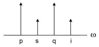
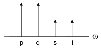
Figure 1: Frequency diagrams for Bragg scattering in a fiber. The long arrows denote strong pumps ($p$ and $q$), whereas the short arrows denote weak sidebands ($s$ and $i$).

BS is described by the sideband amplitudes $A_{s}$ and $A_{i}$. These complex amplitudes are the components of a Jones vector and their spatial evolution is a linear transformation in Jones space. Two complex variables are equivalent to four real variables. However, an inspection of the BS equations shows that one variable is ignorable, so BS can be described by only three real variables, which are the components of a Stokes-like vector. The Stokes-space description of BS is useful because it allows one to visualize power and phase information simultaneously, and because evolution in Stokes space is a simple rotation of the Stokes vector.

This report is organized as follows: In Sec. 2 the coupled equations for the sideband (mode) amplitudes are stated and solved. In Sec. 3 these scalar equations are rewritten as a matrix equation for the Jones vector and their solutions are used to specify the associated transfer matrix. In Sec. 4 the Stokes parameters associated with the sideband amplitudes are defined and the (unknown) elements of a Stokes-space rotation matrix are related to the (known) elements of a Jones-space transfer matrix. An evolution equation for the Stokes vector is also derived and solved directly. In Sec. 5, the Poisson-bracket formalism for BS is developed and shown to be consistent with the Stokes-vector equation. In Sec. 6, the Pauli spin-matrix formalism is used to relate the (unknown) elements of a Jones-space transfer matrix to the (known) elements of a Stokes-space rotation matrix. The mathematics of the bracket and spin-matrix formalisms are similar to the mathematics of angular-momentum operators. Hence, familiarity with the former facilitates the transition from the classical model of BS to the quantal model (which will be described elsewhere). Finally, in Sec. 7 the main results of this report are summarized.

The evolution of a monochromatic wave with two polarization components was described, in Jones space and Stokes space, in [15]. The notation and results of [15] will be used without further comment.

2. Coupled modes

The initial evolution of BS (during which the pumps are not depleted) is governed by the Hamiltonian

$$H=\delta(|A_{s}|^{2}-|A_{i}|^{2})+\gamma A_{s}^{*}A_{i}+\gamma^{*}A_{s}A_{i}^{*},$$ (1)

together with the Hamilton equations

$$d_{z}A_{j}=i\partial H/\partial A_{j}^{*}.$$ (2)

For the case in which the pump and sideband polarizations are parallel, the wavenumber mismatch $\delta=(\beta_{s}+\beta_{q}-\beta_{i}-\beta_{p})/2+\gamma_{K}(|A_{p}|^{2}-|A_{q}|^{2})/2$, where $\beta_{j}=\beta(\omega_{j})$ are wavenumbers, $\gamma_{K}$ is the Kerr coefficient and $A_{p}$ and $A_{q}$ are pump amplitudes, and the coupling coefficient $\gamma=2\gamma_{K}A_{p}A_{q}^{*}$ [8]. Other polarization configurations are discussed in [11, 12]. By combining Eqs. (1) and (2), one obtains the (linear) coupled-mode equations

$$d_{z}A_{s} = i\delta A_{s}+i\gamma A_{i},$$ (3)

$$d_{z}A_{i} = i\gamma^{*}A_{s}-i\delta A_{i}.$$ (4)

Similar equations govern power transfer in a directional coupler [16] and sum-frequency generation in a crystal [17]. Equivalent equations for the sideband powers $P_{j}=|A_{j}|^{2}$ and phases $\phi_{j}=\arg(A_{j})$ are derived in the Appendix.

The solutions of Eqs. (3) and (4) can be written in the input–output form

$$A_{s}(z) = \mu(z)A_{s}(0)+\nu(z)A_{i}(0),$$ (5)

$$A_{i}(z) = -\nu^{*}(z)A_{s}(0)+\mu^{*}(z)A_{i}(0),$$ (6)

where the transfer functions

$$\mu(z) = \cos(kz)+i\delta\sin(kz)/k,$$ (7)

$$\nu(z) = i\gamma\sin(kz)/k$$ (8)

and the BS wavenumber $k=(\delta^{2}+|\gamma|^{2})^{1/2}$. Notice that the transfer functions satisfy the auxiliary equation $|\mu|^{2}+|\nu|^{2}=1$, which is a manifestation of power conservation. The signal-to-idler conversion efficiency $|A_{i}(z)|^{2}/|A_{s}(0)|^{2}$ attains its maximum of $|\gamma|^{2}/k^{2}$ when $kz=\pi/2$.

3. Jones vector

The scalar equations (3) and (4) can be rewritten as the matrix equation

$$d_{z}A=iKA,$$ (9)

where the amplitude (Jones) vector $A=[A_{s},A_{i}]^{t}$ and the coefficient matrix

$$K=\left[\begin{array}[]{cc}\delta&\gamma\\ \gamma^{*}&-\delta\end{array}\right].$$ (10)

Equation (9) has the formal solution

$$A(z)=U(z)A(0),$$ (11)

where the transfer matrix $U=e^{iKz}$. Since $K$ is hermitian, $U$ is unitary. Hence, it can be written in the Caley–Klein form

$$U=\left[\begin{array}[]{cc}\mu&\nu\\ -\nu^{*}&\mu^{*}\end{array}\right],$$ (12)

which is consistent with Eqs. (5) and (6). This result is a manifestation of power conservation. Notice that Eq. (9) is equivalent to the Hamiltonian

$$H=A^{\dagger}KA,$$ (13)

together with the vector Hamilton equation

$$d_{z}A=i\partial H/\partial A^{\dagger}.$$ (14)

4. Stokes vector

Define $A_{j}=P_{j}^{1/2}e^{i\phi_{j}}$, where $P_{j}$ is a sideband power and $\phi_{j}$ is a sideband phase. Then an inspection of Eq. (1) shows that the Hamiltonian depends on the phase difference $\phi_{s}-\phi_{i}$, but not on the total phase $\phi_{s}+\phi_{i}$. Hence, BS can be described in terms of three real variables (not four). For such an interaction, it is natural to introduce the Stokes-like parameters

$$S_{0} = |A_{s}|^{2}+|A_{i}|^{2},$$ (15)

$$S_{1} = |A_{s}|^{2}-|A_{i}|^{2},$$ (16)

$$S_{2} = A_{s}A_{i}^{*}+A_{s}^{*}A_{i},$$ (17)

$$S_{3} = i(A_{s}A_{i}^{*}-A_{s}^{*}A_{i}),$$ (18)

in which the sideband amplitudes $A_{s}$ and $A_{i}$ play the roles of the polarization components $X$ and $Y$ [18]. $S_{0}$ is the total sideband power, $S_{1}$ is the power difference, and $S_{2}$ and $S_{3}$ contain information about the phase difference. Notice that $S_{0}^{2}=S_{1}^{2}+S_{2}^{2}+S_{3}^{2}$.

By combining Eqs. (5) and (6) with Eq. (15), one finds that

$$S_{0}(z)=S_{0}(0).$$ (19)

The total power is conserved because the Hamiltonian does not depend on the total phase, as discussed in the Appendix. This result implies that the Stokes vector $\vec{S}=(S_{1},S_{2},S_{3})$ has constant magnitude, so evolution in Stokes space is rotation on a sphere of radius $S_{0}$ (the Stokes sphere). By combining Eqs. (5) and (6) with Eqs. (16)–(18), one finds that

$$S(z)=R(z)S(0),$$ (20)

where the column vector $S=[S_{1},S_{2},S_{3}]^{t}$ and the rotation matrix

$$R=\left[\begin{array}[]{ccc}(\mu_{r}^{2}+\mu_{i}^{2}-\nu_{r}^{2}-\nu_{i}^{2})&2(\mu_{i}\nu_{i}+\mu_{r}\nu_{r})&2(\mu_{i}\nu_{r}-\mu_{r}\nu_{i})\\ 2(\mu_{i}\nu_{i}-\mu_{r}\nu_{r})&(\mu_{r}^{2}-\mu_{i}^{2}-\nu_{r}^{2}+\nu_{i}^{2})&2(\nu_{r}\nu_{i}+\mu_{r}\mu_{i})\\ 2(\mu_{i}\nu_{r}+\mu_{r}\nu_{i})&2(\nu_{r}\nu_{i}-\mu_{r}\mu_{i})&(\mu_{r}^{2}-\mu_{i}^{2}+\nu_{r}^{2}-\nu_{i}^{2})\end{array}\right].$$ (21)

The identity $|\mu|^{2}+|\nu|^{2}=1$ ensures that $R$ is orthogonal. By combining Eqs. (7), (8) and (21), one obtains the explicit formulas

$$k^{2}R_{11}(\theta) = \delta^{2}+(\gamma_{r}^{2}+\gamma_{i}^{2})\cos\theta,$$ (22)

$$k^{2}R_{12}(\theta) = \delta\gamma_{r}(1-\cos\theta)-\gamma_{i}k\sin\theta,$$ (23)

$$k^{2}R_{13}(\theta) = -\delta\gamma_{i}(1-\cos\theta)-\gamma_{r}k\sin\theta,$$ (24)

$$k^{2}R_{21}(\theta) = \delta\gamma_{r}(1-\cos\theta)+\gamma_{i}k\sin\theta,$$ (25)

$$k^{2}R_{22}(\theta) = \gamma_{r}^{2}+(\gamma_{i}^{2}+\delta^{2})\cos\theta,$$ (26)

$$k^{2}R_{23}(\theta) = -\gamma_{r}\gamma_{i}(1-\cos\theta)+\delta k\sin\theta,$$ (27)

$$k^{2}R_{31}(\theta) = -\delta\gamma_{i}(1-\cos\theta)+\gamma_{r}k\sin\theta,$$ (28)

$$k^{2}R_{32}(\theta) = -\gamma_{r}\gamma_{i}(1-\cos\theta)-\delta k\sin\theta,$$ (29)

$$k^{2}R_{33}(\theta) = \gamma_{i}^{2}+(\delta^{2}+\gamma_{r}^{2})\cos\theta,$$ (30)

where the distance parameter $\theta=2kz$. The evolution of the Stokes vector is illustrated in Fig. 2.

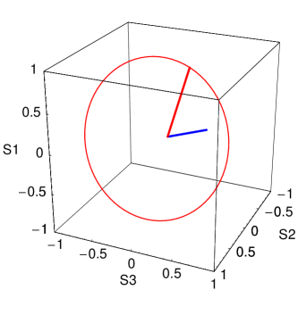
Figure 2: Trajectory of the Stokes vector for $\delta/\gamma_{r}=0.3$ and $\gamma_{i}/\gamma_{r}=0.1$. The thick blue and red lines denote the rotation axis $\vec{r}$ and input Stokes vector $\vec{S}(0)$, respectively. The thin red curve denotes the trajectory of the tip of the Stokes vector.

In the preceding analysis, known results for the mode amplitudes were used to deduce results for the Stokes parameters. However, one can also determine the evolution of the Stokes parameters directly. By combining Eqs. (3) and (4), one obtains the evolution equations

$$d_{z}S_{0} = 0,$$ (31)

$$d_{z}S_{1} = -2\gamma_{i}S_{2}-2\gamma_{r}S_{3},$$ (32)

$$d_{z}S_{2} = 2\delta S_{3}+2\gamma_{i}S_{1},$$ (33)

$$d_{z}S_{3} = 2\gamma_{r}S_{1}-2\delta S_{2}.$$ (34)

Equation (31) is consistent with Eq. (19), and Eqs. (32)–(34) can be rewritten as the vector equation

$$d_{z}\vec{S}=\vec{\Omega}\times\vec{S},$$ (35)

where the rotation vector $\vec{\Omega}=2(-\delta,-\gamma_{r},\gamma_{i})$. [If one were to replace $\gamma$ by $\gamma^{*}$, the rotation vector would be $-2(\delta,\gamma_{r},\gamma_{i})$ and some formulas would be simpler. However, the appearance of $\gamma A_{i}$ in the equation for $A_{s}$ is standard.] Define $\vec{\Omega}=2k\vec{r}$, where the wavenumber $k$ was defined after Eq. (8) and $\vec{r}=(-\delta,-\gamma_{r},\gamma_{i})/k$ is a unit vector parallel to $\vec{\Omega}$. Then $\vec{S}_{\parallel}=\vec{r}(\vec{r}\cdot\vec{S})$ is parallel to the rotation vector, $\vec{S}_{\perp}=\vec{S}-\vec{r}(\vec{r}\cdot\vec{S})$ is perpendicular to the rotation vector and lies in the plane defined by $\vec{r}$ and $\vec{S}$, and the auxiliary vector $\vec{S}_{\times}=\vec{r}\times\vec{S}$ is perpendicular to the rotation vector and the $rs$-plane. If the Stokes vector rotates about $\vec{r}$ through the angle $\theta=2kz$, $\vec{S}_{\parallel}$ remains constant and $\vec{S}_{\perp}$ becomes $\cos\theta\vec{S}_{\perp}+\sin\theta\vec{S}_{\times}$. By combining these facts, one obtains the rotation formula

$$\vec{S}(\theta)=[\cos\theta+(1-\cos\theta)\vec{r}\vec{r}\cdot+\sin\theta\vec{r}\times]\vec{S}(0).$$ (36)

Equation (36) is consistent with Eqs. (22)–(30). The quantity in square brackets is the rotation operator, written in dyadic (rather than matrix) form.

5. Poisson-bracket formalism

Another inspection of Eq. (1) shows that the Hamiltonian

$$H=\delta S_{1}+\gamma_{r}S_{2}-\gamma_{i}S_{3},$$ (37)

where $S_{1}$–$S_{3}$ were defined in Eqs. (16)–(18). This equation can be rewritten in the compact form $H=-\vec{\Omega}\cdot\vec{S}/2$, where $\Omega$ was defined after Eq. (35). Since the Hamiltonian depends only on the Stokes parameters, it is natural to formulate the interaction in Stokes space. For any Stokes parameter $S_{j}$, the rate of change

$$d_{z}S_{j}=\sum_{k}\Biggl{(}{\partial S_{j}\over\partial A_{k}}{dA_{k}\over dz}+{\partial S_{j}\over\partial A_{k}^{*}}{dA_{k}^{*}\over dz}\Biggr{)}.$$ (38)

By combining Eqs. (2) and (38), one obtains the Hamilton equation

$$d_{z}S_{j}=i\{S_{j},H\},$$ (39)

where the Poisson bracket

$$\{P,Q\}=\sum_{k}\Biggl{(}{\partial P\over\partial A_{k}}{\partial Q\over\partial A_{k}^{*}}-{\partial P\over\partial A_{k}^{*}}{\partial Q\over\partial A_{k}}\Biggr{)}.$$ (40)

Notice that $\{Q,P\}=-\{P,Q\}$. Since $H$ depends on $S_{k}$, to determine the consequences of Eq. (39) one must first calculate the Poisson brackets $\{S_{j},S_{k}\}$. The results are

$$\{S_{j},S_{k}\}=\pm 2iS_{l},$$ (41)

where the $+$ ($-$) sign applies if $j$, $k$ and $l$ are in positive (negative) cyclic order. By combining Eqs. (39) and (41), one obtains the evolution equations

$$d_{z}S_{1}=\Omega_{2}S_{3}-\Omega_{3}S_{2},$$ (42)

$$d_{z}S_{2}=\Omega_{3}S_{1}-\Omega_{1}S_{3},$$ (43)

$$d_{z}S_{3}=\Omega_{1}S_{2}-\Omega_{2}S_{1},$$ (44)

which are equivalent to Eq. (35). $S_{0}$ is constant because $\{S_{0},S_{j}\}=0$. The Poisson-bracket formulation of classical mechanics is described in [19].

6. Spin-matrix formalism

In the preceding sections the Stokes-space evolution was described in terms of Jones-space transfer functions [Eqs. (7) and (8)], and directly in Stokes space [Eq. (35)]. In this section the Jones-space evolution is described in terms of Stokes-space quantities.

First, suppose that a Stokes vector is written in the polar form

$$\vec{S}=S_{0}(\cos\theta,\sin\theta\cos\phi,\sin\theta\sin\phi).$$ (45)

Then the associated Jones vector

$$A=S_{0}^{1/2}[\cos(\theta/2)e^{-i\phi/2},\sin(\theta/2)e^{i\phi/2}]^{t}.$$ (46)

One can verify Eq. (46) by combining it with Eqs. (16)–(18) and comparing the results to Eq. (45). Polar coordinates are illustrated in Fig. 3.

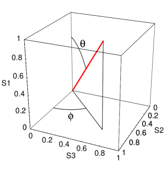
Figure 3: Polar coordinates in Stokes space. The red line denotes the Stokes vector $\vec{S}$.

Second, suppose that a Stokes-space rotation is specified by the rotation axis $\vec{r}$ and angle $\theta$ (which should not be confused with the polar angle of the preceding paragraph). Some analysis is required to relate these quantities to their counterparts in Jones space. In Sec. 3 it was shown that the transfer matrix $U=e^{iKz}$, where $K$ is the coefficient matrix (10). One can facilitate the exponentiation of $iKz$ by defining the identity matrix $\sigma_{0}$ and the Pauli spin matrices

$$\sigma_{1}=\left[\begin{array}[]{cc}1&0\\ 0&-1\end{array}\right],\ \ \sigma_{2}=\left[\begin{array}[]{cc}0&1\\ 1&0\end{array}\right],\ \ \sigma_{3}=\left[\begin{array}[]{cc}0&-i\\ i&0\end{array}\right].$$ (47)

These hermitian matrices have the properties $\sigma_{j}^{2}=\sigma_{0}$ and $\sigma_{j}\sigma_{k}=\pm i\sigma_{l}$, where the $+$ ($-$) sign applies if $j$, $k$ and $l$ are in positive (negative) cyclic order. The latter result implies that $\sigma_{j}\sigma_{k}+\sigma_{k}\sigma_{j}=0$. Furthermore, any complex matrix $M$ can be written in the form

$$M=m_{0}\sigma_{0}+\vec{m}\cdot\vec{\sigma},$$ (48)

where the scalar and vector coefficients $m_{0}={\rm Tr}(\sigma_{0}M)/2$ and $\vec{m}={\rm Tr}(\vec{\sigma}M)/2$, respectively, and the spin vector $\vec{\sigma}=(\sigma_{1},\sigma_{2},\sigma_{3})$. The coefficient matrix has the decomposition

$$K=\delta\sigma_{1}+\gamma_{r}\sigma_{2}-\gamma_{i}\sigma_{3},$$ (49)

which can be rewritten in the compact form $K=-k\vec{r}\cdot\vec{\sigma}$, where $k$ and $\vec{r}$ were defined after Eq. (35). By using the aforementioned properties of the spin matrices, one finds that

$$U(z)=\sigma_{0}\cos(kz)-i\vec{r}\cdot\vec{\sigma}\sin(kz).$$ (50)

By combining Eqs. (12) and (48), one also finds that

$$U=\mu_{r}\sigma_{0}+i(\mu_{i}\sigma_{1}+\nu_{i}\sigma_{2}+\nu_{r}\sigma_{3}).$$ (51)

It follows from Eqs. (49) and (50) that

$$\mu_{r}(z)=\cos(kz),\ \ [\mu_{i}(z),\nu_{i}(z),\nu_{r}(z)]=-\sin(kz)\vec{r},$$ (52)

where $[\mu_{i},\nu_{i},\nu_{r}]$ is a row vector. Equations (52) relate the Jones-space transfer functions to the Stokes-space rotation axis $\vec{r}$ and the distance parameter $kz$. The discussion between Eqs. (35) and (36) shows that $kz=\theta/2$, where $\theta$ is the Stokes-space rotation angle.

The connections between the formulas that describe evolution in Jones and Stokes space are not accidental. It follows from Eqs. (16)–(18) and (47) that

$$S_{j}=A^{\dagger}\sigma_{j}A.$$ (53)

By combining Eqs. (9) and (53), one finds that

$$d_{z}S_{j}=iA^{\dagger}[\sigma_{j},K]A,$$ (54)

where the commutator

$$[P,Q]=PQ-QP.$$ (55)

The spin matrices satisfy the commutation relations

$$[\sigma_{j},\sigma_{k}]=\pm 2i\sigma_{l},$$ (56)

where the $+$ ($-$) sign applies if $j$, $k$ and $l$ are in positive (negative) cyclic order. Equations (56) are the analogs of Eqs. (41) and the identity $[\vec{\sigma},\vec{r}\cdot\vec{\sigma}]=2i\vec{r}\times\vec{\sigma}$ follows from them. By combining this identity with Eq. (54), one obtains the evolution equation

$$d_{z}\vec{S}=2k\vec{r}\times\vec{S},$$ (57)

which is equivalent to Eq. (35). $S_{0}$ is constant because $[\sigma_{0},\sigma_{j}]=0$. Other connections between Jones space and Stokes space are described in [15].

7. Summary

Optical frequency conversion by Bragg scattering (BS) in a fiber was considered. The evolution of BS can be modeled using the signal and idler (sideband) amplitudes [Eqs. (3) and (4)], which are complex, or the sideband powers and phases [Eqs. (60)–(63)], which are real. The amplitudes are the components of a Jones vector and their spatial evolution is a linear transformation in Jones space [Eq. (11)]. However, the Hamiltonian for BS [Eq. (1) or (58)] does not depend on the total sideband phase. This fact has two important consequences. First, BS can be described by only three real variables, which are the components of a Stokes-like vector. The Stokes-space description of BS is useful because it allows one to visualize power and phase information simultaneously. Second, the total sideband power is conserved. In Jones space the norm of the Jones vector is constant, so the transformation is unitary [Eq. (12)], whereas in Stokes space the length of the Stokes vector is constant, so its evolution is rotation [Eq. (36)].

The analysis of BS proceeded in three phases. In the first phase, the coupled equations for the sideband (mode) amplitudes were stated [Eqs. (3) and (4)] and solved [Eqs. (7) and (8)]. These scalar equations were rewritten as a matrix equation for the Jones vector [Eq. (9)] and their solutions were used to specify the associated transfer matrix [Eq. (12)]. The Stokes parameters associated with the mode amplitudes were defined and the (unknown) elements of a Stokes-space rotation matrix were related to the (known) elements of a Jones-space transfer matrix [Eq. (21)]. In the second phase, an evolution equation for the Stokes vector was derived [Eq. (35)], which confirmed that evolution in Stokes space is rotation. This equation has a concise solution [Eq. (36)], which relates the rotation axis and angle to the mismatch and coupling coefficients, and the distance. The Poisson-bracket formalism for BS was developed [Eq. (39)] and shown to be consistent with the Stokes-vector equation [Eqs. (42)–(44)]. In the third phase, the Pauli spin-matrix formalism was used to solve the Jones-vector equation [Eq. (50)]. This solution is consistent with the solutions of the coupled-mode equations and relates the (unknown) elements of a Jones-space transfer matrix to the (known) elements of a Stokes-space rotation vector [Eq. (52)]. Thus, explicit formulas were derived, which relate the Jones and Stokes pictures of BS. The power-phase formulation of the BS equations is described in the Appendix.

The mathematics of the bracket and spin-matrix formalisms are similar to the mathematics of angular-momentum operators. Hence, familiarity with the former facilitates the transition from the classical model of BS to the quantal model (which will be described in a future report).

Acknowledgment

I thank H. Kogelnik for his constructive comments on the manuscript.

Appendix: Phase plane

Section 2 was based on the complex formulation of the Hamilton function (1) and equations (2). This appendix is based on the associated real formulation. Define $A_{j}=P_{j}^{1/2}e^{i\phi_{j}}$ and $\gamma=|\gamma|e^{i\phi_{\gamma}}$. Then the initial evolution of BS is governed by the Hamiltonian

$$H=\delta(P_{s}-P_{i})+2|\gamma|(P_{s}P_{i})^{1/2}\cos(\phi_{s}-\phi_{i}-\phi_{\gamma}),$$ (58)

together with the Hamilton equations

$$d_{z}P_{j}=-\partial H/\partial\phi_{j},\ \ d_{z}\phi_{j}=\partial H/\partial P_{j}.$$ (59)

The assumption that $\gamma$ is real is equivalent to the assumptions that $\phi_{s}$ and $\phi_{i}$ are measured relative to $\phi_{\gamma}/2$ and $-\phi_{\gamma}/2$, respectively. By combining Eqs. (58) and (59), one obtains the power equations

$$d_{z}P_{s} = 2\gamma(P_{s}P_{i})^{1/2}\sin(\phi_{s}-\phi_{i}),$$ (60)

$$d_{z}P_{i} = -2\gamma(P_{s}P_{i})^{1/2}\sin(\phi_{s}-\phi_{i})$$ (61)

and the phase equations

$$d_{z}\phi_{s} = \delta+\gamma(P_{i}/P_{s})^{1/2}\cos(\phi_{s}-\phi_{i}),$$ (62)

$$d_{z}\phi_{i} = -\delta+\gamma(P_{s}/P_{i})^{1/2}\cos(\phi_{s}-\phi_{i}).$$ (63)

It follows from Eqs. (60) and (61) that the total power $P_{t}=P_{s}+P_{i}$ is conserved (because $H$ depends on $\phi_{s}-\phi_{i}$). It also follows from Eqs. (60)–(63) that $H$ is constant (because it does not depend explicitly on $z$).

Define the power difference $p=(P_{s}-P_{i})/P_{t}$, phase difference $\phi=\phi_{s}-\phi_{i}$ and Hamiltonian $h=H/(\gamma P_{t})$. In the notation of Sec. 4, $p=S_{1}/S_{0}$ and $\phi$ is the angle between the projection of $\vec{S}$ on the 23-plane and the 2-axis (Fig. 3). Furthermore, let $\delta/\gamma\rightarrow\delta$ and $2\gamma z\rightarrow z$. Then BS is governed by the normalized Hamiltonian

$$h=\delta p+(1-p^{2})^{1/2}\cos\phi,$$ (64)

together with the normalized Hamilton equations

$$d_{z}p=-\partial h/\partial\phi,\ \ d_{z}\phi=\partial h/\partial p.$$ (65)

By combining Eqs. (64) and (65), one obtains the normalized power and phase equations

$$d_{z}p = (1-p^{2})^{1/2}\sin\phi,$$ (66)

$$d_{z}\phi = \delta-p\cos\phi/(1-p^{2})^{1/2},$$ (67)

respectively. Equations (66) and (67) are consistent with Eqs. (60)–(63).

Phase diagrams associated with the Hamiltonian (64) are shown in Fig. 4. The phase point $(p,\phi)$ moves in such a way that an observer moving with it, and looking forward, keeps higher energies on his left. For $\delta=0.0$ the trajectories are librations. The trajectory that starts at the point $(-\pi/2,1)$ is a straight line to $(-\pi/2,-1)$, followed by a phase jump to $(\pi/2,-1)$, followed by a straight line to ($\pi/2,1)$, followed by a jump back to $(-\pi/2,1)$. For $\delta=0.3$ some trajectories are librations, whereas others are rotations. The trajectory that starts at $(-\pi/2,1)$ is a curve to the point $(\pi/2,1)$, followed by a phase jump back to $(-\pi/2,1)$, and the trajectory that starts at $(-\pi/2,-1)$ is a curve to the point $(\pi/2,-1)$, followed by a jump back to $(-\pi/2,-1)$.

     

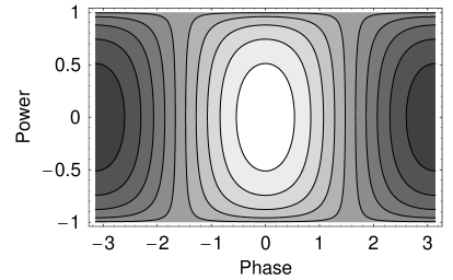
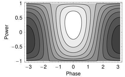
Figure 4: Phase diagram for ($a$) $\delta/\gamma=0.0$ and ($b$) $\delta/\gamma=0.3$. Lighter regions correspond to higher energies, whereas darker regions correspond to lower energies. The energy contours (solid curves) are the trajectories of the phase point $(p,\phi)$.

These phase diagrams describe the evolution of BS qualitatively. To describe the evolution quantitatively, one must solve Eqs. (66) and (67). First, suppose that $\delta=0$, which corresponds to (left-handed) rotation about the 2-axis in Stokes space. Then

$$(d_{z}p)^{2} = (1-p^{2})\sin^{2}\phi,$$ (68)

$$= 1-h^{2}-p^{2}.$$

It follows from Eq. (68) that

$$p(z)=(1-h^{2})^{1/2}\cos(z+z_{0}),$$ (69)

where $h$ is constant and the distance parameter $z_{0}=\cos^{-1}[p(0)/(1-h^{2})^{1/2}]$. For the case in which $\delta=0$ and $\gamma_{i}=0$, Eqs. (20), (22) and (24) can be rewritten in the normalized form

$$s_{1}(z)=s_{1}(0)\cos z-s_{3}(0)\sin z.$$ (70)

By using the identity $s_{3}^{2}+s_{1}^{2}=1-s_{2}^{2}$, one finds that $s_{1}(0)=(1-s_{2}^{2})^{1/2}\cos z_{0}$ and $s_{3}(0)=(1-s_{2}^{2})^{1/2}\sin z_{0}$, where $s_{2}=h$ and $z_{0}=\tan^{-1}[s_{3}(0)/s_{1}(0)]$ is the angle between the projection of $\vec{S}(0)$ on the 31-plane and the 1-axis. Hence,

$$s_{1}(z)=(1-s_{2}^{2})^{1/2}\cos(z+z_{0}).$$ (71)

Equation (71) is equivalent to Eq. (69).

Second, suppose that $\delta\neq 0$, which corresponds to (left-handed) rotation about the axis $(\delta,1,0)/k$, where $k=(1+\delta^{2})^{1/2}$. Then

$$(d_{z}p)^{2} = 1-p^{2}-(h-\delta p)^{2},$$ (72)

$$= k^{2}[p_{d}^{2}-(p-p_{a})^{2}],$$

where the power average $p_{a}=\delta h/k^{2}$ and power difference $p_{d}=(k^{2}-h^{2})^{1/2}/k^{2}$. In the notation of Sec. 4, $p_{a}=r_{1}(\vec{r}\cdot\vec{S})$ and $p_{d}=|\vec{S}_{\perp}(0)|/k$. It follows from Eq. (72) that

$$p(z)=p_{a}+p_{d}\cos[k(z+z_{0})],$$ (73)

where $kz_{0}=\cos^{-1}\{[p(0)-p_{a}]/p_{d}\}$. For the case in which $\gamma_{i}=0$, Eqs. (20) and (22)–(24) can be rewritten in the normalized form

$$k^{2}s_{1}(z) = s_{1}(0)[\delta^{2}+\cos(kz)]+s_{2}(0)\delta[1-\cos(kz)]-s_{3}(0)k\sin(kz),$$ (74)

$$= \delta[\delta s_{1}(0)+s_{2}(0)]+[s_{1}(0)-\delta s_{2}(0)]\cos(kz)-ks_{3}(0)\sin(kz),$$

where $\delta s_{1}(0)+s_{2}(0)=h$. By using the identity $s_{1}^{2}+s_{2}^{2}+s_{3}^{2}=1$, one finds that $[s_{1}(0)-\delta s_{2}(0)]^{2}+[ks_{3}(0)]^{2}=k^{2}-h^{2}$. Hence, Eq. (74) can be rewritten in the form of Eq. (73), with $kz_{0}=\tan^{-1}\{ks_{3}(0)/[s_{1}(0)-\delta s_{2}(0)]\}$. The nonlinear evolution of BS is described in [5, 9].

References

[1] J. Hansryd, P. A. Andrekson, M. Westlund, J. Li and P. O.
Hedekvist, “Fiber-based optical parametric amplifiers and their
applications,” IEEE J. Sel. Top. Quantum Electron. 8,
506–520 (2002).
[2] C. J. McKinstrie, S. Radic and A. H. Gnauck, “All-optical
signal processing by fiber-based parametric devices,” Opt. Photon.
News 18 (3), 34–40 (2007).
[3] G. G. Luther and C. J. McKinstrie, “Transverse modulational
instability of counterpropagating light waves,” J. Opt. Soc. Am. B
9, 1047–1060 (1992). Bragg reflection of counter-propagating
sidebands is discussed.
[4] M. Yu, C. J. McKinstrie and G. P. Agrawal,
“Instability due to cross-phase modulation in the normal dispersion
regime,” Phys. Rev. E 48, 2178–2186 (1993). Bragg scattering
of co-propagating sidebands is mentioned.
[5] C. J. McKinstrie, X. D. Cao and J. S. Li, “Nonlinear detuning
of four-wave interactions,” J. Opt. Soc. Am. B 10, 1856–1869
(1993). If the four-wave equations are solved for three inputs with
arbitrary strengths, the solutions apply to both Bragg scattering
and phase conjugation.
[6] K. Inoue, “Tunable and selective wavelength conversion using
fiber four-wave mixing with two pump lights,” IEEE Photon. Technol.
Lett. 6, 1451–1453 (1994).
[7] M. E. Marhic, Y. Park, F. S. Yang and L. G. Kazovsky, “Widely
tunable spectrum translation and wavelength exchange by four-wave
mixing in optical fibers,” Opt. Lett. 21, 1906–1908 (1996).
[8] C. J. McKinstrie, S. Radic and A. R. Chraplyvy, “Parametric
amplifiers driven by two pump waves,” IEEE J. Sel. Top. Quantum
Electron. 8, 538–547 and 956 (2002).
[9] K. Uesaka, K. K. Y. Wong, M. E. Marhic and L. G.
Kazovsky, “Wavelength exchange in a highly nonlinear
dispersion-shifted fiber: Theory and experiments,” IEEE J. Sel.
Top. Quantum Electron. 8, 560–568 (2002).
[10] T. Tanemura, C. S. Goh, K. Kikuchi and S. Y. Set,
“Highly efficient arbitrary wavelength conversion within entire
C-band based on nondegenerate fiber four-wave mixing,” IEEE Photon.
Technol. Lett. 16, 551–553 (2004).
[11] C. J. McKinstrie, H. Kogelnik, R. M. Jopson, S. Radic and
A. V. Kanaev, “Four-wave mixing in fibers with random
birefringence,” Opt. Express 12, 2033–2055 (2004).
[12] C. J. McKinstrie, H. Kogelnik and L. Schenato,
“Four-wave mixing in a rapidly-spun fiber,” Opt. Express 14,
8516–8534 (2006). This paper also reviews four-wave mixing in
strongly-birefringent and randomly-birefringent fibers.
[13] A. H. Gnauck, R. M. Jopson, C. J. McKinstrie, J. C.
Centanni and S. Radic, “Demonstration of low-noise frequency
conversion by Bragg scattering in a fiber,” Opt. Express 14,
8989–8994 (2006).
[14] D. Méchin, R. Provo, J. D. Harvey and C. J. McKinstrie,
“180-nm wavelength conversion based on Bragg scattering in an
optical fiber,” Opt. Express 14, 8995–8999 (2006).
[15] J. P. Gordon and H. Kogelnik, “PMD fundamentals: Polarization
mode dispersion in optical fibers,” Proc. Nat. Acad. Sci. 97,
4541–4550 (2000).
[16] H. Kogelnik, “Theory of optical waveguides,” in Guided-Wave
Optoelectronics, 2nd Ed., edited by T. Tamir (Springer, 1990),
Chapter 2.
[17] R. W. Boyd, Nonlinear Optics (Academic
Press, 1992), Chapter 2.
[18] J. D. Jackson, Classical Electrodynamics, 2nd.
Ed. (Wiley, 1975), Chapter 7.