On the equilibrium rotation of Earth-like extra-solar planets

The equilibrium rotation of tidally evolved “Earth-like” extra-solar planets is often assumed to be synchronous with their orbital mean motion. The same assumption persisted for Mercury and Venus until radar observations revealed their true spin rates. As many of these planets follow eccentric orbits and are believed to host dense atmospheres, we expect the equilibrium rotation to differ from the synchronous motion. Here we provide a general description of the allowed final equilibrium rotation states of these planets, and apply this to already discovered cases in which the mass is lower than 12 $M_{\oplus}$. At low obliquity and moderate eccentricity, it is shown that there are at most four distinct equilibrium possibilities, one of which can be retrograde. Because most presently known “Earth-like” planets present eccentric orbits, their equilibrium rotation is unlikely to be synchronous.

1 Introduction

After a significant number of discoveries of new extra-solar gaseous giant planets, a new barrier has been passed with the detections of several planets in the Neptune and even Earth-mass ($M_{\oplus}$) regime: $5-12$ $M_{\oplus}$ (Rivera et al., 2005; Lovis et al., 2006; Udry et al., 2007; Bonfils et al., 2007). If the commonly accepted core-accretion model can account for the formation of these planets, resulting in a mainly icy/rocky composition, the fraction of the residual He-H₂ atmospheric envelope accreted during the planet migration is not tightly constrained for planets more massive than the Earth (e.g. Alibert et al., 2006). A minimum mass of below 10 $M_{\oplus}$ is usually considered to be the boundary between terrestrial and giant planets, but Rafikov (2006) found that planets more massive than 6 $M_{\oplus}$ could have retained more than 1 $M_{\oplus}$ of the He-H₂ gaseous envelope. For comparison, masses of Earth’s and Venus’ atmosphere are respectively $\sim 10^{-6}$ and $10^{-4}$ times the planet’s mass. Despite significant uncertainties, these discoveries of “super-Earths” provide an opportunity to test some properties that could be similar to those of our more familiar telluric planets.

Because some of these planets are potentially in the “habitable zone” (Udry et al., 2007; Selsis et al., 2007), their spin state is an important factor in understanding their climate. For planets with a negligible atmosphere such as Mercury, solid tides induced by the host star are expected to despin the planet until an equilibrium position or a capture in a spin-orbit resonance, depending on the orbital eccentricity and the permanent quadrupole moment of inertia (Goldreich & Peale, 1966; Correia & Laskar, 2004). However, for planets with dense atmosphere such as Venus, thermal atmospheric tides, driven by solar insolation, have a profound influence on the spin, and may destabilize the previous tidal equilibrium state. Correia & Laskar (2001, 2003b) investigated the combined effect of gravitational and atmospheric tides on Venus and showed that the planet could evolve into two different final states, the existing retrograde motion being the most probable one. This study was performed with the small eccentricity approximation that may no longer be adequate for “Earth-like” planets, which exhibit a wide range of eccentricities, orbital distances, or central star types. Following the work of Laskar & Correia (2004), we generalize here these previous studies and investigate the possible equilibrium rotation states of “Earth-like” planets in the presence of significant eccentricity. Although our knowledge of these planets is restricted to their orbital parameters and minimum masses, we attempt to place new constraints on their surface rotation rate, assuming that they have a dense atmosphere.

2 Tidal evolution

Tidal effects are generated by differential and inelastic deformation of a planet by a perturbing body. For a planet with a dense atmosphere, we consider the traditional gravitational tides ($\tau=g$), and also thermal atmospheric tides ($\tau=a$) produced by the stellar heating of the atmosphere. In both cases, the averaged variation in the spin can be expressed by the variables that characterize the spin (the rotation rate $\omega$ and the obliquity $\varepsilon$), and the elliptical elements, with semi-major axis $a$ and eccentricity $e$ (e.g. Kaula, 1964; Correia & Laskar, 2003a):

$$\frac{dL}{dt}=T_{\tau}=K_{\tau}\sum_{\sigma}b_{\tau}(\sigma)\Lambda_{\tau,\sigma}(e,\varepsilon)\ ,$$ (1)

where $L=C\omega$ is the angular momentum of the planet, $C$ is the polar moment of inertia, the sum being taken over different harmonics of the tidal frequency $\sigma$ (an integer combination of the rotation rate $\omega$ and the mean motion $n$), $K_{\tau}$ is a factor related to the strength of the tide, $b_{\tau}(\sigma)$ is an odd function related to the dissipation within the planet, and $\Lambda_{\tau,\sigma}$ are polynomial functions of $e$ and $\cos\varepsilon$. Since discovered Earth-like planets have moderate eccentricities (typically $e<0.25$), we neglect terms in $e^{4}$, which allows us to simplify the tidal torques acting on the planet. In the same way, we consider that the planet’s obliquity $\varepsilon$ is small, neglecting terms higher than $\varepsilon^{2}$ in Eq.(1).

Gravitational tides are raised on the planet by the star because of the effect of the gravitational gradient across the planet. Equation (1) becomes (eg. Kaula, 1964):

$$T_{g} = \frac{3}{2}K_{g}\left[\left(1-5e^{2}\right)\,b_{g}(2\omega-2n)\phantom{\frac{1}{1}}\right.$$ (3)

$$\left.+\frac{1}{4}\,e^{2}b_{g}(2\omega-n)+\frac{49}{4}\,e^{2}b_{g}(2\omega-3n)\right]\ ,$$

where $K_{g}=-GM_{*}^{2}R^{5}/a^{6}$, $G$ is the gravitational constant, $M_{*}$ is the mass of the star, and $R$ is the mean radius of the planet. Since planets are not perfectly rigid, there will be a distortion that produces a tidal bulge of amplitude $k_{2}$, the second order potential Love number. Imperfect elasticity delays the planet’s response to the perturbation by a time lag $\Delta t_{g}$. The deformation therefore lag behind the perturbation by an angle $\delta_{g}=\sigma\Delta t_{g}/2$ and $b_{g}(\sigma)=\!k_{2}\!\sin 2\delta_{g}=k_{2}\sin\left(\sigma\Delta t_{g}\right)$ (e.g. Correia & Laskar, 2003a).

The differential absorption of the stellar heat by the planetary atmosphere gives rise to local variations in temperature and consequently to pressure gradients. The mass of the atmosphere is then redistributed, adjusting for an equilibrium position. Observations on Earth show that the pressure redistribution is essentially a superposition of two pressure waves: a diurnal tide of small amplitude (with no dynamical counterpart) and a strong semi-diurnal tide (see Chapman & Lindzen, 1970). As for gravitational tides, the redistribution of mass in the atmosphere produces an atmospheric bulge that modifies the gravitational potential generated by the atmosphere. The resulting tidal torque is (Dobrovolskis & Ingersoll, 1980; Correia & Laskar, 2003a):

$$T_{a} = \frac{3}{2}K_{a}\left[\left(1-3e^{2}\right)\,b_{a}(2\omega-2n)\right.$$ (5)

$$\left.-\,e^{2}b_{a}(2\omega-n)+9\,e^{2}b_{a}(2\omega-3n)\right]\ ,$$

where $K_{a}=-3M_{*}R^{3}/(5\rho a^{3})$, and $\rho$ is the mean density of the planet. The amplitude of the bulge is given by $\tilde{p}_{2}$, the second order surface pressure variations (Chapman & Lindzen, 1970):

$$\tilde{p}_{2}(\sigma)=\mathrm{i}\frac{\gamma}{\sigma}\tilde{p}_{0}\left(\nabla\cdot\@vec{v}_{\sigma}-\frac{\gamma-1}{\gamma}\frac{J_{\sigma}}{gH_{0}}\right)=\mathrm{i}\frac{\cal P_{\sigma}}{\sigma}\ ,$$ (6)

where $\gamma=7/5$ for a perfect diatomic gas, $\tilde{p}_{0}$ is the mean surface pressure, $\@vec{v}$ is the velocity of tidal winds, $J$ is the amount of heat absorbed or emitted by a unit mass of air per unit time, and $H_{0}$ is the scale height at the surface. There is also a delay $\Delta t_{a}$ before the response of the atmosphere to the stellar heat excitation. However, the imaginary number in Eq.(6) causes the pressure variations to lead the Sun ($\mathrm{i}=e^{\mathrm{i}\pi/2}$). Using $\delta_{a}=\sigma\Delta t_{a}/2$, we thus have $b_{a}(\sigma)=\tilde{p}_{2}\sin 2\delta_{a}=|\tilde{p}_{2}|\sin 2(\delta_{a}+\pi/2)=-|\tilde{p}_{2}|\sin 2\delta_{a}$.

The dependence of time lags on the tidal frequency is poorly known for gravitational and atmospheric tides. For a review of the different dissipation models, see Correia et al. (2003). For both tides we adopt the simplest model for slow rotation (i.e. the viscous model), as described by Mignard (1979), where a constant time lag is assumed for all components of the tidal perturbation. Since we usually have $\sigma\Delta t\ll 1$, this model can be made linear:  $b_{g}(\sigma)\simeq k_{2}\,\sigma\Delta t_{g}\quad\mathrm{and}\quad b_{a}(\sigma)\simeq-|\tilde{p}_{2}|\,\sigma\Delta t_{a}$. For atmospheric tides, it is also necessary to consider the response of the surface pressure variations to tidal frequency (Eq. 6). We use the “heating-at-the-ground model” described by Dobrovolskis & Ingersoll (1980). It is supposed that all the stellar flux absorbed by the ground, $F_{s}$, is immediately deposited in a thin layer of atmosphere at the surface. The heating distributing is then written as a delta-function just above the ground ($J_{\sigma}=gF_{s}/\tilde{p}_{0}$). This approximation is justified because tides in the upper atmosphere are decoupled from the ground by the disparity between their rotation rates and it appears to be in good agreement with the observations. Neglecting $\@vec{v_{\sigma}}$ over the thin heated layer, Eq.(6) becomes: ${\cal P_{\sigma}}=F_{s}/(8H_{0})\propto L_{*}/a^{2}$ ($L_{*}$ is the star luminosity).

The average evolution of the rotation rate is obtained by adding the effects of both tidal torques acting on the planet, that is $\dot{\omega}=(T_{a}+T_{g})/C$. Substituting dissipative models described above in Eqs.(3) and (5) then leads to

$$\dot{\omega}/K_{0} = \omega-\left(1+6e^{2}\right)n-\omega_{s}\left[\left(1-3e^{2}\right)\mathrm{sign}(\omega-n)\right.$$ (8)

$$\left.-\,e^{2}\mathrm{sign}(2\omega-n)+9\,e^{2}\mathrm{sign}(2\omega-3n)\right]\ ,$$

where $K_{0}=-3\Omega(e)K_{g}k_{2}\Delta t_{g}/C$, $\;\,\Omega(e)=1+15e^{2}/2$,

$$\omega_{s}=\frac{F_{s}}{8H_{0}\Omega(e)k_{2}}\frac{K_{a}\Delta t_{a}}{K_{g}\Delta t_{g}}\propto\frac{L_{*}}{M_{*}}\,\frac{R}{m}\,a\ ,$$ (9)

and $m$ is the planet mass. According to Eq.(6), atmospheric tides are weak during the first stages of evolution ($\sigma\gg n$). Gravitational tides alone can therefore be used to estimate the characteristic time needed to reach the equilibrium rotation, $\tau_{eq}$:

$$\tau_{eq}^{-1}\sim\left|K_{0}\right|=\frac{3k_{2}\,\Delta t_{g}\,R^{5}}{C\,G}\,n^{4}\sim\frac{9\,G\,M_{*}^{2}\,k_{2}\,\Delta t_{g}\,R^{3}}{m\,a^{6}}\ ,$$ (10)

with $C\simeq m\,R^{2}/3$. All terrestrial extra-solar planets listed in Table 1 have a despinning timescale that is significantly lower than the age of the system ($<10^{7}$ yrs), so we expect that they have already reached their equilibrium rotation state.

3 Equilibrium final states for the rotation rate

An equilibrium final state is achieved when $\dot{\omega}=0$, that is for $T_{g}=-T_{a}$. When $e=0$, we derive:

$$f(\omega-n)=-\frac{T_{g}}{T_{a}}=-\frac{K_{g}b_{g}(2\omega-2n)}{K_{a}b_{a}(2\omega-2n)}=1\ ,$$ (11)

where $f(x)$ is an even function of $x$ (Correia & Laskar, 2001). Assuming that $f(x)$ is monotonic close to the equilibrium (which is true for the usual dissipation models), we have

$$|\omega-n|=f^{-1}(1)\equiv\omega_{s}\ ,$$ (12)

i.e. there are two final possibilities for the equilibrium rotation of the planet, given by $\omega^{\pm}=n\pm\omega_{s}$, where $2\pi/\omega_{s}$ can be seen as the synodic period. Unless $\omega_{s}\ll n$, the synchronous motion ($\omega=n$) is no longer the final equilibrium position for Earth-like planets tidally evolved. According to Correia & Laskar (2001, 2003b), the planet is free to evolve to any of the two final equilibrium positions, although it appears to have a preference for the slowest one ($\omega^{-}=n-\omega_{s}$). If $\omega_{s}<n$, both final states correspond to prograde final rotation rates (Fig.1b,c). However, if $\omega_{s}>n$, the slowest rotation rate becomes negative, corresponding to a retrograde configuration. This is the present situation of the planet Venus for which $\omega_{s}/n=1.92$ (Fig.1a).

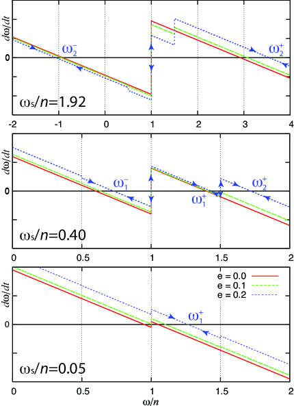
Figure 1: Evolution of $\dot{\omega}$ (Eq. 8) with $\omega_{s}/n=1.92$, $\omega_{s}/n=0.40$ and $\omega_{s}/n=0.05$, for different eccentricities ($e=0.0,0.1,0.2$). The equilibrium rotation rates are given by $\dot{\omega}=0$ and the arrows indicate whether it is a stable or unstable equilibrium position. For $\omega_{s}/n>1$, we have two equilibrium possibilities, $\omega^{\pm}_{2}$, one of which corresponds to a retrograde rotation (as for Venus). For $\omega_{s}/n<1$, retrograde states are not possible, but we can still observe final rotation rates $\omega^{-}<n$. For eccentric orbits, because of the terms in $b_{\tau}(2\omega-n)$ and $b_{\tau}(2\omega-3n)$, we may have at most four different final possibilities (Eq.16). When $\omega_{s}/n$ becomes extremely small, which is the case for the present observed extra-solar planets with some eccentricity (Table 1), a single final equilibrium is possible for $\omega^{+}_{1}$.

When $e\neq 0$, Eq.(12) is no longer valid and additional equilibrium positions for the rotation rate may occur. For moderate values of the eccentricity, we can write from Eqs.(3) and (5):

$$f(\omega-n)=1+e^{2}\left(2+\frac{g(\omega)}{b_{a}(2\omega-2n)}\right)\ ,$$ (13)

where

$$g(\omega) = \frac{K_{g}}{4K_{a}}\left[b_{g}(2\omega-n)+49b_{g}(2\omega-3n)\right]$$ (15)

$$-\,b_{a}(2\omega-n)+9\,b_{a}(2\omega-3n)\ .$$

Since $b_{\tau}(\sigma)$ are monotonic odd functions, the effect of the eccentricity is eventually to split each previous equilibrium rotation rate into two new equilibrium values so that four final equilibrium positions for the rotation rate are possible, written as:

$$\omega^{\pm}_{1,2}=n\pm\omega_{s}+e^{2}\,\delta^{\pm}_{1,2}\ ,$$ (16)

with

$$\delta^{\pm}_{1,2}=\left(2+\frac{g(\omega)}{|b_{a}(2\omega-2n)|}\right)\left.\frac{\partial f^{-1}}{\partial x}\right|_{x=1}\ ,$$ (17)

or, adopting the tidal models described in Sect. 2 (Eq. 8):

$$\delta^{-}_{1,2}=6n-\left(6\pm 1\right)\omega_{s}\quad\mathrm{and}\quad\delta^{+}_{1,2}=6n-\left(4\pm 9\right)\omega_{s}\ ,$$ (18)

where $+$ corresponds to the state $\delta_{1}$ and $-$ to the state $\delta_{2}$. Because the set of $\omega^{\pm}_{1,2}$ values must verify the additional condition

$$\omega^{-}_{2}<n/2<\omega^{-}_{1}<n<\omega^{+}_{1}<3n/2<\omega^{+}_{2}\ ,$$ (19)

these four equilibrium rotation states cannot, in general, exist simultaneously, depending on the values of $\omega_{s}$ and $e$. In particular, the final states $\omega^{-}_{1}$ and $\omega^{+}_{1}$ can never coexist with $\omega^{-}_{2}$. At most three different equilibrium states are therefore possible, obtained when $\omega_{s}/n$ is close to $1/2$, or more precisely, when $1/2-17\,e^{2}/2<\omega_{s}/n<1/2+7\,e^{2}/2$. Conversely, we found that one single final state $\omega^{+}_{1}=(1+6e^{2})\,n+(1-13e^{2})\,\omega_{s}$ exists when $\omega_{s}/n<6e^{2}(1-7e^{2})$.

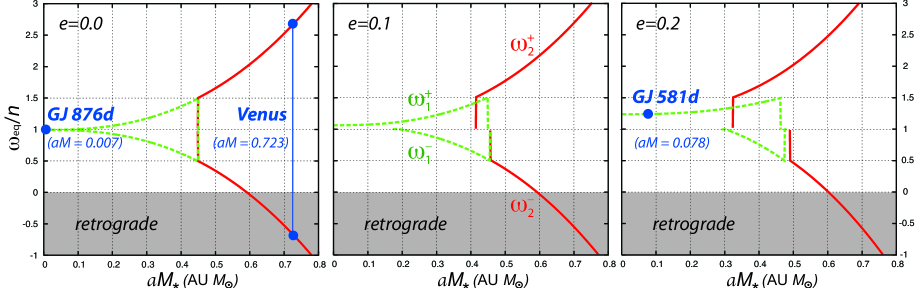
Figure 2: Equilibrium positions of the rotation rate as a function of the product $aM_{*}$ for three different values of the eccentricity ($e=0.0,0.1,0.2$). Each curve corresponds to a different final state (dotted lines for $\omega_{1}^{\pm}$ and solid lines for $\omega_{2}^{\pm}$). For $e\simeq 0$ (case of Venus), we always count two final states that are symmetrical about $n$. For small values of $aM_{*}$, the two equilibrium possibilities are so close to $n$ that the most likely scenario for the planet is to be captured in the synchronous resonance (case of GJ 876 d). As we increase the eccentricity, we can count at most three final equilibrium rotations, depending on the value of $\omega_{s}/n$ (computed from Eq. 20). When $e\simeq 0.2$, only one equilibrium state exists for $aM_{*}<0.3$, resulting from $\omega_{s}/n<6e^{2}(1-7e^{2})$. This is the present situation of GJ 581 d and most of the “Earth-like” extra-solar planets listed in Table 1.

Table 1: Characteristics and equilibrium rotation rates of Earth-like planets with masses lower than $12\,M_{\oplus}$ (see text for notations).

Name	$M_{*}$	Age	${}^{*}\tau_{eq}$	$m\sin i$	$a$	$e$	$\omega_{s}/n$	$2\pi/n$	$2\pi/\omega^{-}_{1}$	$2\pi/\omega^{-}_{2}$	$2\pi/\omega^{+}_{1}$	$2\pi/\omega^{+}_{2}$
	[$M_{\odot}$]	[Gyr]	[Gyr]	$[m_{\oplus}]$	[AU]			[day]	[day]	[day]	[day]	[day]
Venus	1.00	4.5	2.3	0.82	0.723	0.007	1.92	224.7		$-$243		76.8
GJ 581 c1	0.31	4.3	$10^{-5}$	5.0	0.073	0.16	0.0002	12.93			11.2
GJ 876 d2	0.32	9.9	$10^{-8}$	5.7	0.021	0	$10^{-5}$	1.9378	1.9379		1.9377
GJ 581 d1	0.31	4.3	0.04	7.7	0.253	0.2	0.0026	83.6			67.4
HD 69830 b3	0.86	4-10	$10^{-5}$	10.2	0.079	0.10	0.0009	8.667			8.17
GJ 674 b4	0.35	0.1-1	$10^{-7}$	11.7	0.039	0.2	$10^{-5}$	4.693			3.79
HD 69830 c3	0.86	4-10	$10^{-3}$	11.8	0.186	0.13	0.0069	31.56			28.5

^∗ Using Eq.(10) with $k_{2}=1/3$ and $\Delta t_{g}=640$ s (Earth’s values); References: [1] Udry et al. (2007); [2] Rivera et al. (2005); [3] Lovis et al. (2006); [4] Bonfils et al. (2007). Earth-like planets OGLE-2005-BLG-390Lb (Beaulieu et al., 2006) and MOA-2007-BLG-192-Lb (Bennett et al., 2008) have not been included because their despinning timescales $\tau_{eq}\sim 10^{2}$ Gyr are much larger than the age of the Universe.

4 Application to Earth-like extra-solar planets

The Earth and Venus are the only Earth-like planets for which the atmosphere and spin are known. Only Venus is tidally evolved and therefore suitable for applying the above expressions for tidal equilibrium. We can nevertheless investigate the final equilibrium rotation states of the already detected “super-Earths”. For that purpose, we considered only the 6 extra-solar planets of masses smaller than 12 $M_{\oplus}$ that we classified as rocky planets with a dense atmosphere, although we stress that this mass boundary is quite arbitrarily. Using the empirical mass-luminosity relation $L_{*}\propto M_{*}^{4}$ (eg. Cester et al., 1983) and the mass-radius relationship for terrestrial planets $R\propto m^{0.274}$ (Sotin et al., 2007), Eq.(9) can be written as:

$$\omega_{s}/n=k\,(a\,M_{*})^{2.5}m^{-0.726}\ ,$$ (20)

where $k$ is a proportionality coefficient that contains all the constant parameters, but also the parameters that we are unable to constrain such as $H_{0}$, $k_{2}$, $\Delta t_{g}$ or $\Delta t_{a}$. In this context, as a first order approximation, we consider that for all these terrestrial planets, the parameter $k$ has the same value as for Venus. Assuming that the rotation of Venus is presently stabilized in the $\omega^{-}$ final state, that is, $2\pi/\omega^{-}=-243$ days (Carpenter, 1970), we compute $2\pi/\omega_{s}=116.7$ days. Replacing it in Eq.(20), we find for Venus that $k=3.32\;m_{\oplus}^{0.726}M_{\odot}^{-2.5}$AU^-2.5. We can then estimate the ratio $\omega_{s}/n$ for all considered extra-solar planets in order to derive their respective equilibrium rotation rates (Table 1). The number and values of the equilibrium rotation states are plotted as a function of $aM_{*}$ for different eccentricities in Fig. 2. All eccentric planets have a ratio $\omega_{s}/n$ that is lower than $7\times 10^{-3}$, which verifies the condition $\omega_{s}/n<6e^{2}(1-7e^{2})$. As a consequence, only one single final state $\omega^{+}_{1}/n\simeq(1+6\,e^{2})$ exists, corresponding to the equilibrium rotation induced by gravitational tides only (Eq. 3). The main reason is that the effect of atmospheric tides is clearly disfavored relative to the effect of gravitational tides on Earth-like planets discovered orbiting M-dwarf stars: The smaller orbital distance strengthens the effect of gravitational tides, which are proportional to $1/a^{6}$, while the effect of thermal tides varies as $1/a^{5}$. Moreover, the smaller mass of the central star also strongly affects the luminosity received by the planet and hence the size of the atmospheric bulge driven by thermal contrasts.

The only exception is GJ 876 d, because its eccentricity is believed to be zero (yet to be confirmed). However, the two equilibrium rotation states $\omega^{\pm}_{1}$ are so close to the mean motion $n$, that the quadrupole moment of inertia (not included in our analysis) will probably capture the rotation in synchronous resonance.

5 Discussion and conclusion

We have derived a simple model that permits the determination of the final equilibrium rotation of “Earth-like” planets. Our model contains some uncertain parameters related to the dissipation within the planets, but we were able to gather all this information in a single parameter, $\omega_{s}$. By varying this, we can then cover all possibilities for the rotation of terrestrial planets. We demonstrated that for a planet of moderate eccentricity and low obliquity, at most four final equilibrium positions are possible. For eccentricities higher than $e\sim 0.5$, terms of higher degree in $e$ should be considered in Eq.(3) that may generate additional equilibrium positions.

Based on the present rotation of Venus, we provided an estimate of $\omega_{s}$ for different environments (Eq. 20). An important consequence is that the ratio $\omega_{s}/n$ increases rapidly with the semi-major axis and mass of the star because $\omega_{s}/n\propto(aM_{*})^{2.5}$. The effect of the atmosphere on the equilibrium rotation is therefore more relevant for planets that orbit Sun-like stars at not close distances. Unfortunately, this situation is precisely the opposite of that for the discovered Earth-like planets (Table 1), since the radial velocity technique is more sensitive to the detection of short-period planets. As a consequence, unlike Venus, none of these planets can be stabilized with a rotation rate $\omega<n$, because for $e>0.1$ these final states only exist if $aM_{*}>0.2$ AU $M_{\odot}$ (Fig.2). The effect of atmospheric tides is extremely small ($\omega_{s}/n\sim 0$) and the equilibrium rotation is essentially driven by the tidal gravitational torque. However, their significant eccentricity ($0.1<e<0.2$) moves the equilibrium position away from the synchronous motion. Capture in this resonance is unlikely, but capture in a higher order spin-orbit resonance cannot be rejected, in particular for GJ 581 d and GJ 674 b, depending on the asymmetry of their mass distribution.