The Micro-Arcsecond Scintillation-Induced Variability (MASIV) Survey II: The First Four Epochs

Abstract

We report on the variability of 443 flat spectrum, compact radio sources monitored using the VLA for 3 days in 4 epochs at $\sim 4$ month intervals at 5 GHz as part of the Micro-Arcsecond Scintillation-Induced Variability (MASIV) survey. Over half of these sources exhibited 2-10% rms variations on timescales over 2 days. We analyzed the variations by two independent methods, and find that the rms variability amplitudes of the sources correlate with the emission measure in the ionized Interstellar Medium along their respective lines of sight. We thus link the variations with interstellar scintillation of components of these sources, with some (unknown) fraction of the total flux density contained within a compact region of angular diameter in the range 10-50$\mu$as. We also find that the variations decrease for high mean flux density sources and, most importantly, for high redshift sources. The decrease in variability is probably due either to an increase in the apparent diameter of the source, or a decrease in the flux density of the compact fraction beyond $z\sim 2$. Here we present a statistical analysis of these results, and a future paper will the discuss the cosmological implications in detail.

1 Introduction

The discovery of centimeter-wavelength Intra-Day Variability (IDV) or “flickering” in Active Galactic Nuclei (AGN) by Heeschen (1984) initially raised concerns that some AGN possess brightness temperatures over six orders of magnitude above the $10^{12}\,$K inverse Compton limit for incoherent synchrotron emission (e.g. Quirrenbach et al., 1989). However, considerable evidence has now accumulated to demonstrate that interstellar scintillation (ISS) in the turbulent, ionized interstellar medium (ISM) of our Galaxy is the principal mechanism responsible for the IDV observed in AGN, as was proposed by Heeschen & Rickett (1987).

Two more recent observational techniques provide compelling evidence for the prevalence of ISS. Time delays of 1–8 min are observed in the arrival times of the flux density variations between telescopes on different continents for the three intra-hour variable sources B0405–385, B1257–326 and J1819$+$3845 (Jauncey et al., 2000; Bignall et al., 2006; Dennett-Thorpe & de Bruyn, 2002). The delay arises due to the finite time required for the stochastic fluctuations associated with the ISM to drift across the Earth. A second observational signature of ISS relates to the modulation of IDV variability timescales with a period of exactly one year. This arises because the Earth’s orbital motion about the Sun contributes to the effective velocity with which the interstellar scattering material moves relative to an Earth-bound observer; the variations are slow as the Earth moves parallel to the material and fast as it moves anti-parallel to it. Annual cycles in IDV variability timescales are reported in at least seven sources (e.g. Dennett-Thorpe & de Bruyn, 2003; Rickett et al., 2001; Jauncey & Macquart, 2001; Bignall et al., 2003; Jauncey et al., 2003), including several whose long variability timescales preclude detection of time delays in the scintillation pattern over intercontinental distances. For many lines of sight through the ISM the slowest variations are expected in September if the motion of the turbulent material is comparable to the local standard of rest (LSR).

The recognition of ISS as the dominant cause of IDV has not entirely alleviated the brightness temperatures problems posed by these sources. A source must be small to scintillate; in the weak scintillation case most frequently observed at frequencies near 5 GHz (Walker, 1998), the source angular size must be comparable to or smaller than the angular size of the first Fresnel zone, $\theta_{\rm F}=\sqrt{c/2\nu\pi L}$. Here $L$ is the distance to the scattering region, which we will refer to as the screen even though in some cases it may be better described as a slab extending from the Earth out to distance $\sim L$. $\theta_{\rm F}$ is typically tens of microarcseconds for screen distances of tens to hundreds of parsecs, which implies source components with angular sizes two to three orders of magnitude finer than the scales probed by VLBI. The long time-scale over which IDV has been observed in some sources suggests that such scintillating components can be relatively long-lived despite their small physical sizes.

This paper reports on the results of a Micro-Arcsecond Scintillation-Induced Variability (MASIV) survey for IDV in AGN. This year-long survey conducted observations of between 500–700 AGN over each of four epochs of three or four days duration in 2002 and 2003 at 4.9 GHz with the VLA. The aim of the survey was to provide a catalogue of at least 100 AGN which vary on timescales of hours to days to provide the basis of detailed studies of the IDV AGN population drawn from a well-defined sample. A description of the observations in epochs 2, 3 and 4 is presented in §2 as a supplement to descriptions of the first epoch observations and MASIV source selection in Lovell et al. (2003) (hereafter Paper 1). In §3 we describe how the time series of flux density for each source in each epoch was classified as variable or non-variable. In §4 we describe how we have quantified the amplitude and timescale for the variations from an analysis of the structure function combined from all 4 epochs and apply corrections for noise and other sources of flux density error. The basic hypothesis of the paper that the variations are predominantly due to interstellar scintillation is presented and examined in §5, including the influence of parameters of the interstellar medium (§5.1 emission measure and galactic latitude) and of the sources themselves (§5.2 mean flux density, spectral index). We now have redshifts for more than half of the sources and we present the dependence of the variability on redshift in §5.5 - a result which shows that the MASIV survey provides a new cosmological probe. In §5.6 we consider whether the variability is intermittent over the four epochs. Our data are listed in Table 4 and our conclusions are presented in §6.

2 Observations and Data Reduction

The VLA observations took place over four periods during January, May and September 2002 and January 2003 (see Table 1). All epochs were 72 hours in duration except September 2002, which included an additional 24 hours. The additional time in this epoch was added as an attempt to detect the slower variation expected in September due to interstellar scintillation caused by material moving at a velocity comparable to the LSR.

All observations took place during array reconfiguration and in each case the array was being moved to a more compact configuration (except for epoch #1). In each epoch the VLA was divided into five independent subarrays. In the first epoch each subarray observed a subset of the 710 source sample. Subarrays 1 through 4 observed the “core” 578 sources of our compact, flat spectrum sample (Lovell et al., 2003), namely the weak ($105<S_{\rm 8.6\,GHz}<130$ mJy) and strong ($S_{\rm 8.6\,GHz}>600$ mJy) sub-samples, while the fifth subarray observed a sample of intermediate flux density sources in two regions of the sky. For the next three epochs all sources previously observed in subarrays 1 through 4 were reobserved, thus providing full coverage for the core sample. However, subarray 5 was re-dedicated to observing a smaller number of sources comprising all objects found to be variable in subarray 5 during the first epoch, as well as the most rapid variables found during the first epoch which required faster sampling in order to determine time scales. In this paper we compare results for the core sample from subarrays 1 through 4 only.

Shadowing was a serious concern at low elevations in the more compact VLA configurations. The impact of shadowing was minimized by assigning 5 or 6 antennas to each subarray in such a way that at any given time a source could be observed with at least 3 unshadowed antennas. Any data from baselines containing shadowed antennas were flagged. Antennas that had either not moved during reconfiguration or were moved but had pointing solutions already applied were assigned to subarrays 1 to 4 where possible.

The core sample was divided into four roughly equal parts by Declination and a subarray assigned to each. The Declination ranges for the four subarrays were $0^{\circ}\leq\delta<14^{\circ}$, $14^{\circ}\leq\delta<34.08^{\circ}$, $34.08^{\circ}\leq\delta<49^{\circ}$, $\delta\geq 49^{\circ}$. The Declination boundary between the second and third subarray was set to the latitude of the VLA to avoid long slews in azimuth when changing between sources transiting north and south of the zenith.

Each subarray was scheduled so that every source was observed for one minute every $\sim$2 h while it was above an elevation of $15^{\circ}$. We used the standard VLA frequency configuration for continuum 4.9 GHz observations (dual polarisation and two 50 MHz bandwidth IFs per polarisation) and a 3.3 s integration time. For flux density calibration, each subarray observed B1328+307 (3C286) and J2355+4950 every $\sim$ 2 hours. B1328+307 is the primary flux density calibrator for the VLA and J2355+4950 is a GPS source, not likely to vary over short timescales, and is monitored regularly at the VLA as part of a calibrator monitoring program.

Following the observations we calibrated the data in AIPS using the standard technique for continuum data. The task FILLM was used to load the data where corrections were made for known antenna gain variations as a function of elevation and for atmospheric opacity. Upon inspection of the data it was clear that there were residual time-dependent amplitude calibration errors. We ascribe this to the fact that in each epoch, some VLA antennas had recently been moved and their pointing calibration observations were not complete. The residual pointing errors may depend on azimuth and elevation so we chose several bright, non-variable sources in each subarray at a range of RA as gain calibrators for surrounding sources. Precautions were taken to ensure that the calibrators themselves were not variable: if a given calibrator caused the majority of sources against which it was applied to vary, then another calibrator was chosen. These sources, typically recommended VLA calibrators, were drawn from our source sample. The numbers of sources used as secondary calibrators in the four epochs were 42, 33, 20 and 36. On the epochs that a particular source was used as a calibrator, it is by definition non-variable and was excluded from the structure function analysis discussed below.

Following calibration, the data for each source were inspected and occasional outlying samples were flagged. The data were then incoherently averaged on a one-minute timescale over all baselines. For all sources, the formal errors obtained were less than those estimated due to the residual constant and fractional errors discussed later in this paper. Incoherent averaging was chosen because, on the assumption that all sources are unresolved, the phase should be zero and any residual phase errors in the data would artificially reduce the average flux density. In low signal-to-noise regimes an incoherent average can induce an upward bias, as visibility amplitudes follow a Rice distribution, which has a mean that is systematically higher than the true mean (Thompson et al., 2001). In the case of our observations though, the signal-to-noise ratio of our observations is sufficiently high that this effect is negligible

As the VLA array configurations became more compact, our data became more sensitive to extended structure in the source and in nearby objects. The changing response of the VLA with time due to this structure can appear as variability in a light curve. Fortunately, as our observations were scheduled in sidereal time and were repeated at the same times every day, false variability due to structure appears as a repeating pattern with a period of one day. In general this was easy to recognise but in some cases imaging was carried out to verify contaminating structure. For the purposes of our analysis, such sources were removed from our sample. A total of 102 sources were removed due to structure or confusion, and one was removed due to an error in our initial sample selection process. Following these removals, we are left with a sample of 475 point sources common to all four epochs.

3 Classification of Variables

We used two separate approaches to analyze the flux density variations. This section describes how we classified the sources based on the apparent modulation index of their intensity. The following section describes a structure function analysis. The virtues of these two techniques are complementary: the first is based on a conservative but robust criterion of source variability, while the second uses a simple statistical estimator which allowed us to quantify the amplitude and time scale of the variations.

In order to ascertain whether an individual source is variable it is necessary to understand the sources of error inherent to the measurements. There are uncertainties in the individual measurements due to calibration errors causing a fractional error, $p$, and additive errors, $s$, due to thermal noise and confusion. Calibration errors include contributions from antenna pointing errors, system gain variation between the observations of flux calibrators and variable atmospheric absorption. Since they are a small percentage of the mean source flux density, $\bar{S}$, they can be approximated as additive and added in quadrature to the noise as given by

$$\sigma_{{\rm err},s,p}=\sqrt{(s/\bar{S})^{2}+p^{2}}\,.$$ (1)

Here $\sigma_{{\rm err},s,p}$ is the rms error in each flux density estimate normalized by the mean for each epoch. In our initial analysis (Paper I) we estimated $s=1.5$ mJy and $p=0.01$.

An initial inspection classified sources based on a their modulation index, defined as the rms of the three days observations divided by the mean flux density, computed for each epoch. A source was identified as variable if its modulation index exceeded twice the expected contribution from the measurement errors, $2\sigma_{{\rm err},s,p}$, as in a $\chi^{2}$ test. However, direct inspection of the data revealed that many of the slower variables, that is sources with variability time-scales longer than three days, were not detected as variable using this criterion.

We therefore introduced an alternative variability criterion, which classified a source as variable if the modulation index of its daily average flux densities exceeded $2\sigma_{\rm err}$. This process yielded more detections, but visual inspection again revealed that many sources that clearly exhibited variability were undetected by either test. In particular, examination revealed that our two criteria do not detect variability in those sources with low-level monotonic flux density changes during the 3-4 d duration of our observations. This is because the $\chi^{2}$ statistic used in our two selection criteria is not an ordered statistic and is therefore sub-optimal in detecting such a low level trend.

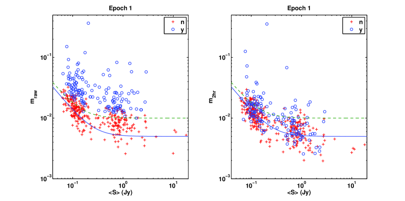
Figure 1: Left: Raw modulation index for epoch 1 plotted against mean source flux density. Sources classified as variable plotted as circles and non-variable as pluses. Right: Similar plot for $m_{2{\rm h}}$ as described and defined in §4.1. In both plots the dashed line is equation(1) with $s=0.0015$ Jy and $p=0.01$ and the solid line has $s=0.0013$ Jy and $p=0.005$. Similar plots are obtained for the other three epochs.

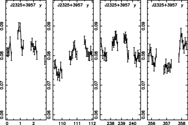
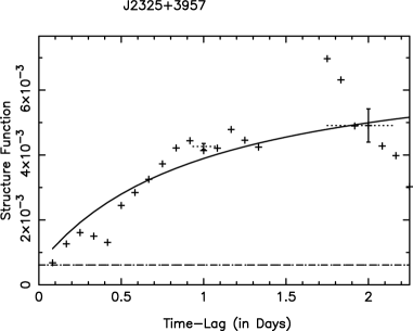
Figure 2: Upper: Time series of flux density (Jy) for J2325+3957 versus day number from 2002 January 1; error bars are as in Paper 1. Lower: Structure Function $D(\tau)$ of flux density (normalized by its mean) averaged over all 4 epochs. The dashed line is the estimated noise level $D_{\rm noise}$ and the solid line is a simple model fit (see §4.3). The vertical bar centered near lag of 2 d is an estimate of $D(\mbox{2\,day})$ and its standard error.

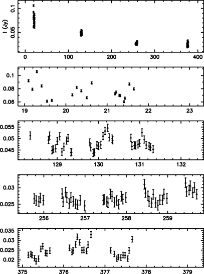
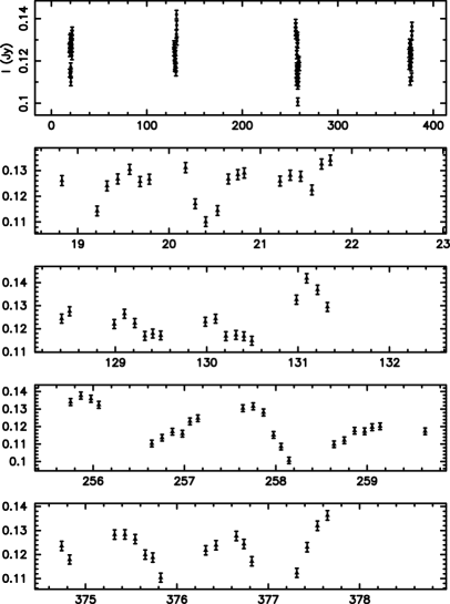
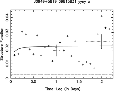
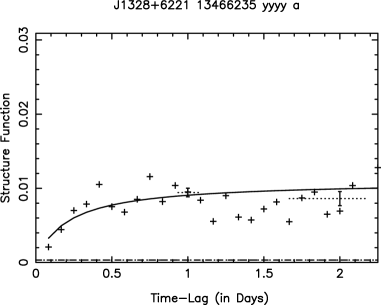
Figure 3: Examples of MASIV variability. J0949+5819 (left) and J1328+6221 (right). The top panel in each case shows all the flux densities in Jy against day number from 2002 January 1. The middle four panels show light-curves for each of the first four epochs. The horizontal scale is the same (four days) in each case. Lower panels show structure function of flux density (normalized by its mean) averaged over all 4 epochs. Dashed line is the estimated noise level $D_{\rm noise}$ and the solid line is a simple model fit (see text). J0949+5819 shows evidence of episodic scintillation, possibly related to intrinsic source changes as there appears to be a corresponsence between mean flux density over an epoch and amplitude of scintillation. J1328+6221 shows strong, consistent scintillation over all four observation epochs.

Our selection criteria were therefore augmented with a visual inspection of the remaining light curves. Inspection was performed by two of us independently and the results compared. Each source was considered non-variable unless otherwise demonstrated, and any source where there was disagreement on its classification was reviewed; we adopted the conservative approach of classifying as non-variable any source is which no final agreement was reached on the classification. In the left panel of Figure 1 we show a scatter plot of the raw modulation index $m_{\rm raw}$ of all sources against their mean flux density from epoch 1, using differing symbols for variables and non-variables. The predicted error in a single flux density measurement from equation (1) is shown by the dashed line, which roughly separates the variable from non-variable classifications. This emphasizes that our classification is determined largely by $m_{\rm raw}$. Table 4 lists all the raw modulation indices and variability classifications of all the sources and Figures 2 and 3 show some sample light-curves from the survey.

In Table 2 we list the number of sources classified as variable in zero, one, two, three or all four observing epochs and associated percentages. In this table and in all of what follows we define a set of 443 sources from the 475 sources that excludes those used as secondary calibrators in two or more epochs. Note that 12% of the sources were seen to vary during all four epochs. With any analysis of a large number of observations, however, false positives, i.e. sources that are incorrectly classified as variable, are a significant concern. Since the visual classification was very close to the two sigma criterion, our variability classification is reliable with $\sim 95$% confidence. Thus we give in columns 3 and 4 the predicted fraction of sources misclassified based on the null hypothesis that all 443 sources are non-variable. Evidently these are negligibly small relative to the observed fractions of variables in two or more epochs.

The large numbers of sources classified as variable on multiple epochs firmly establishes that our classification process is reliable. If all 443 sources were non-variable, then the number expected to be classified variable on 2, 3 or 4 epochs is a mere 6.7 or 1.4%, compared with the observed 192 (43%). Even if our classification was 90% reliable, then the number of false positives with 2 or more detections remains less than 5%.

The fraction of sources that can be reliably classified as variable can be deduced using Table 2. Denoting $N$ as the actual number of non-variable sources, $T$ the actual number of one-time variables and $F$ the number of non-variables misclassified as one-time variables, then the apparent number of non-variables $161=N-F$ and from Table 2, $F/N=0.172$. This yields $N=194,F=33$ and hence $T=90-F=56$, and the corrected total number of variables is 192+56=248. Therefore the fraction of sources that exhibited variability in one or more epochs in our survey is 56%. This value is significantly higher than the 15-20% found in previous IDV surveys (Quirrenbach et al., 1992; Kedziora-Chudczer et al., 2001a). In comparing with other surveys one must be careful to consider the selection criteria applied. As described in §2 we started with 710 sources selected from spectral index and mean flux density criteria which was reduced to 443, when we excluded those used as calibrators in more than one epoch and those exhibiting resolution effects, raising the percentage of variable sources. In addition the large number of one-, two- and three-time variable sources raises the percentage. We believe that this is due to intermittency in the IDV phenomenon, which we describe by a simple model in §5.6.

For the purposes of subsequent analysis we conservatively define as “non-variable” those 161 sources that showed no variability in any of the four epochs, and we define as “variable” those 192 sources that showed variability on two or more of the four epochs. With these definitions we have two large and reliable samples each of approximately 200 sources, where the non-variables act as a control sample for the variables. Each was drawn from the same selection criteria and cover the same overall area of sky.

4 Structure Function of the Variations

Here we discuss how we quantify the flux density variation for each source using the structure function (SF) of each time series,

$$D(\tau)=\frac{1}{N_{\tau}}\Sigma_{j,k}(S_{j}-S_{k})^{2}$$ (2)

where $S_{j}$ is a flux density measurement normalized by the mean flux density of the source over all four epochs and $N_{\tau}$ is the number of pairs of flux densities with a time lag $\tau$ binned in 2-hour increments. The SF is a statistically reliable estimator which can be modeled even for short data spans. It is defined independent of any variability classification. Examples are shown in the lower panels of Figure 2 and 3. The SF is preferable to the autocorrelation function for short data spans, which can be badly biased by a poor estimation of the mean.

For an idealized observation of stationary stochastic variations spanning a time much longer than their characteristic time $\tau_{\rm char}$, $D(\tau)$ rises with time lag and tends to saturation at twice the true variance. However for our observations $\tau_{\rm char}$ is typically more than two days and saturation is rarely seen. We thus chose $D(\tau=2\,{\rm d})$ as a standard characterization of the intra-day variations because $\tau=2\,$d is the maximum lag out to which our structure functions contain reliable information for the 72 hour observing sequences. Note that we estimate $D(\tau=2\,{\rm d})$ by combining data from all four epochs, which makes it a more stable statistic under the hypothesis of stationary stochastic variations. Hence we do not use this statistic to determine whether a source’s variability differs over the four epochs.

4.1 Measurement errors

Additive flux density errors that are independent of the ISS (or intrinsic) variations contribute an additive term to the SF. If the errors are independent from one sample to the next (i.e. “white”), the error contribution to SF would have a mean value $D_{\rm noise}=2\sigma_{\rm err}^{2}$ independent of time lag. While random pointing errors will be white, there may be non-white errors caused by systematic pointing errors due to recent antenna relocations and residuals of gain and atmospheric variation, which may contribute a term that is a function of time lag. Nevertheless we now proceed by assuming that all the errors are white and thus the errors add a constant ($D_{\rm noise}$) (plus random variations about the constant due to estimation error) and postpone discussion of possible non-white measurement errors.

Our goal is to subtract $D_{\rm noise}$ from the raw SF $D(\tau)$ in order to estimate the SF of any true variations in a source’s flux density. But first we must consider how best to estimate $D_{\rm noise}$. One estimate is $2\sigma_{\rm err}^{2}$ from equation (1), which depends on the constants $s$ and $p$. Another estimate of $D_{\rm noise}$ comes from the SF itself – evaluated at its shortest time lag (2h). This would be an unbiased estimate for $D_{\rm noise}$ if all real flux density variation had time scales much longer than 2 h. Hence we examined single-epoch estimates of $D(t=2{\rm h})$, which we plot as an equivalent modulation index $m_{2{\rm h}}=\sqrt{0.5D(t=2{\rm h})}$ in the right panel of Figure 1. The sources classified as variable include a substantial number with large values of $m_{2{\rm h}}$, which are due to rapid flux density variations stronger than expected for noise. Note in particular the highest point which is quasar J$1819+3845$ which shows large amplitude rapid ISS. Its timescale is typically shorter than our 2 h sampling and so its SF has already saturated at 2 h and its variations are “white” in our sampling. Similarly the other sources with elevated $m_{2{\rm h}}$ are probably due to ISS with short time scales.

Now consider the non-variables, which are plotted as pluses and provide a set of sources with low or zero variation in epoch 1, which are useful in studying the noise processes. In the right panel of Figure 1 the mean of the plus symbols lies significantly below the dashed line (equation (1) with $s=0.0015$ Jy and $p=0.01$) particularly for the higher flux density sources. The solid line with $s=0.0013$ Jy and $p=0.005$ provides a better model for the noise as discussed in §4.2. In the absence of any real variations the estimates $m_{2{\rm h}}$ should be scattered equally above and below their mean value. Comparing the right and left hand panels we see that $m_{\rm raw}$ is typically higher than $m_{2{\rm h}}$ even for the non-variables, which suggests that $m_{\rm raw}$ is increased due to low level variations with a timescale longer than 2 h.

The discussion above reduces the choice for estimating $D_{\rm noise}$ to either $D(2{\rm~{}h})$ or the value corresponding to the solid line $D_{{\rm err},s,p}=2\sigma_{\rm err}^{2}$ with $p=0.005$. Whereas it is appealing to use the observable $D(2{\rm h})$, any rapid real flux density variations can contribute to $D(2{\rm~{}h})$ which thus overestimates $D_{\rm noise}$. Thus we adopted $D_{{\rm err},s,p}$ as an estimator for $D_{\rm noise}$, which states that the measurement errors are well described by equation(1) but with calibration errors contributing at a 0.5% rather than a 1% level. However we discuss a slight revision of this in the next section.

4.2 Structure Function Correction and Fitting

For each source at each epoch we computed the raw SF as defined in equation (2). As the time lag increases the number of available lagged products ($N_{\tau}$) drops and so increases the error in the SF. A threshold for plotting an estimate for $D(\tau)$ was set at $N_{\tau}>20$% of the total number of data samples in that epoch. As the example in Figure 2 shows, this gives estimates clustered at lags 2-8 h and near 24 h and near 48 h. In order to characterize the variability amplitudes we initially estimate the SF at a lag of 2 d from the mean SF and its estimated error, calculated using the values at lags in the range $\tau=48\pm 2\,$hours. The overplotted model is described in §4.3.

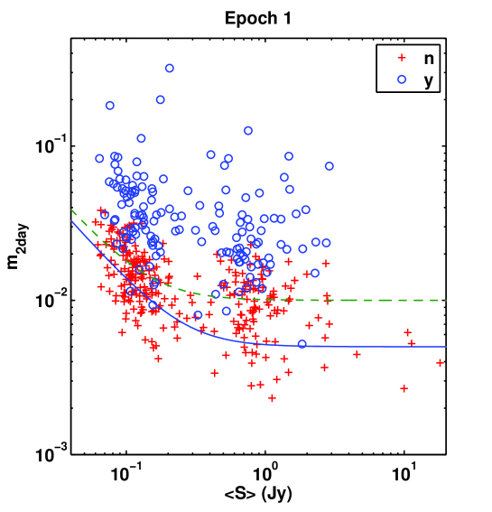
Figure 4: $m_{2\,{\rm d}}=\sqrt{D(2\,{\rm d})}$ (without any noise subtraction) plotted against mean source flux density. Circles are sources classified as variables and pluses as non-variables. The lines are equation(1) with $s=0.0015$ Jy and $p=0.01$ for the dashed line and $s=0.0013$ Jy and $p=0.005$ for the solid line. Similar plots are obtained for the other three epochs.

First consider the equivalent 2-day modulation index $m_{2\,{\rm d}}=\sqrt{0.5D(2\,{\rm d})}$ (without noise correction) plotted against the mean source flux density $\bar{S}$ for epoch 1 in Figure 4. It should be compared with the left and right panels of Figure 1 for the non-variable sources. The comparison makes it clear that $m_{2\,{\rm d}}>m_{2\,{\rm h}}$ for almost all of the non-variable sources. Indeed there is a close correspondence between $m_{2\,{\rm d}}$ and $m_{\rm raw}$. Thus it is clear that there are low level flux density variations on a timescale longer than 2 h in the sources classified as non-variable. In order to investigate what causes these we examined the difference $\Delta D=D(2\,{\rm d})-D(2\,{\rm h})$ for the non-variable sources from each epoch.

We examined how $\Delta D$ depends on mean flux density, Galactic latitude and H$\alpha$ emission – quantities which we find in §5 influence $D(2\,{\rm d})$ for the variable classifications. The results showed that the mean of $\Delta D$ in each epoch was significantly higher for the sources weaker than 0.4 Jy than for those stronger than 0.4 Jy. However, it showed no significant dependence on Galactic latitude or H$\alpha$ emission. Hence the process responsible for the low-level variability in the sources classified as non-variable is not ISS and is unlikely to have an astrophysical origin.

We consider the most likely cause to be confusion, which can be due either to extended source structure which is partially resolved on the baselines of each sub-array or to low level confusing sources in the primary beam. We had already eliminated obvious cases of confusion by removing sources whose light curves showed clear daily patterns of variability which repeated in each day of a 3 day sequence. Since our SF estimation is from the light curves normalized by $\bar{S}$ an increase in $\Delta D$ at low $\bar{S}$ is consistent with the effect of low level confusion characterized by a certain rms in Jy. This is supported by the VLA documentation that gives 2.3 mJy as the brightest source expected in a single antenna beam at 5 GHz.

We examined the shape of the mean $D(\tau)$ for high and low $\bar{S}$ sources in each epoch. Evidence for the effects of confusion was found in the consistent minima in $D(\tau)$ near time lags $\tau=$ 1d and 2d. However, there was also a component rising from the noise floor at 2h and typically saturating between 12 and 24h. All three components were substantially larger for the weak group of sources than for the strong sources. When averaged over four epochs the noise floor was, respectively, at $\sim 3.0\times 10^{-4}$ and $\sim 0.61\times 10^{-4}$ and the averages for $\Delta D$ were, respectively, $\sim 2.8\times 10^{-4}$ and $\sim 1.1\times 10^{-4}$ for these groups (mean flux density 0.13 Jy and 1.4 Jy). By equating these average SF amplitudes to $2\sigma_{err}^{2}$ using equation (1) we estimated $s=0.0013$ Jy and $p=0.0073$. The $s$ values for each epoch ranged from 0.001-0.002 Jy and for $p$ 0.003-0.01, but no consistent patterns were seen versus epoch.

We also considered the effect of long-term variations as characterized by the variation between epochs of the mean flux density from each epoch. These slower variations are mostly intrinsic and might contribute to a trend within the 3 or 4 days of each epoch. So we calculated the rate of change of flux density from the average of the magnitude of the differences in flux density between neighbouring epochs, divided by the number of days between epochs and the resulting magnitude of $D(2{\rm d})$ due to such a trend. Surprisingly, for all sources this was smaller than the noise-corrected $D(2{\rm d})$ except for those which were negative as a result of noise subtraction. Further the highest of them was 0.0001, which is one quarter of the threshold value. So we conclude that long-term variations did not make a significant contribution to the variations observed within the epochs. We note, however, that we can usefully estimate the structure function on time lags of 3 and 6 months from the MASIV survey data, which may be useful in studies of intrinsic variability. Thus we include the epoch averaged flux density for each epoch in the data table 4.

The foregoing studies reveal that the apparently non-variable light curves include not only white noise but also a low level contaminating process whose rms values can be approximately characterized by equation (1). While we can quantify the white noise process by this equation, the non-white contamination is not well enough understood to be reliably characterized by an SF which could be subtracted from the estimates for all sources at each epoch. So in order to reduce the effect of these non-white variations, we increased the estimated $D_{\rm noise}$ to to be subtracted by using the values $s=0.0013$ Jy and $p=0.007$, and we also set a threshold on $D(2\,{\rm d})=4\times 10^{-4}$ below which the noise-corrected SF values may be contaminated and therefore should only be interpreted as upper limits to the true SF of flux density variations.

It is of interest that, since confusion effects will be precisely repeated at 24 h intervals, the samples of the structure function at 24 and 48 hr will be unaffected by confusion. The results we present in subsequent sections are from fitting the SF over all time lags, since the fit makes better use of the data. However, we also analyzed the single sample estimates of $D(24{\rm h})$ and $D(48{\rm h})$ and found very similar results, though with somewhat worse statistical errors. As an extra precaution we re-reviewed all the light curves and SF plots for 24 h periodic patterns and found 34 sources that might be contaminated at a level near the threshold. For these sources we used the lower of $D(2\,{\rm d})$ from the fit and that estimated from $48\pm 2$ h.

4.3 Variability Timescales

Although we estimated the SF as described above for each source at each epoch, the single-epoch $D(2\,{\rm d})$ is only based on about one independent sample of a 2 d variation and so it has a large statistical error – such that its rms error is about equal to its mean (Rickett et al., 2000). Thus we do not attempt to evaluate the variability amplitude on a source by source basis for each of the epochs. Rather we average the SF for each source over all 4 epochs (after subtracting the $D_{\rm noise}$ as defined in the previous section). Hence the SF results are insensitive to any intermittency or annual changes in ISS due to the effects of the Earth’s velocity.

We then fitted the following simple model to the SFs:

$$D(\tau)=2m^{2}\frac{\tau}{\tau+\tau_{\rm char}},$$ (3)

where $2m^{2}$ is the amplitude at which the function would saturate and $\tau_{\rm char}$ is the characteristic timescale where the SF reaches half of its saturation. The motivation for this form is described in Appendix A. It approximates the form expected from ISS caused by a turbulent interstellar medium uniformly distributed through a thick scattering region, as opposed to turbulence confined to a thin layer (see equation(A4)). We estimated two parameters only: the timescale $\tau_{\rm char}$ and the value of $D(\tau=2\,\mbox{d})$ for each source. It should also be noted that a light curve that is dominated by a linear trend in flux density gives rise to a parabolic SF, which is not well fitted by equation (3). The value of $D(\tau=2\,\mbox{d})$ in such a case will be somewhat underestimated.

An example of fitted SF is shown in Figure 2. The points show $D(\tau)$ increasing (noisily) with time lag $\tau$ but not reaching saturation. Since the timescale is defined at half the saturation value it is poorly constrained in this example: $\tau_{\rm char}=1.0\pm 0.5$ days. However, from the same fit $D(t=2\,\mbox{d})=(44\pm 3)\times 10^{-4}$, which is quite well constrained. With observations limited to 3 days (4 days for epoch 3) it is not possible to estimate timescales longer than about 3 days. However, in those cases it was possible to recognize that the characteristic timescale is longer than 3 days from the shape of the structure function. Two other examples are shown in Figure 3, in which there is evidence for faster variations. For source J0949+5819 the variations are very strong in epoch 1 and much weaker in epoch 3. From the epoch-average we find $\tau_{\rm char}=0.02\pm 0.05$ days and $D(t=2\,\mbox{d})=(19\pm 2)\times 10^{-3}$. For J1328+6221 the variations are more consistent over the epochs with $\tau=0.2\pm 0.2$ days and $D(t=2\,\mbox{d})=(10\pm 1)\times 10^{-3}$. Given our 2 hr sampling and the typically large fractional errors in the timescale we have simply classified the timescale into fast $\tau_{\rm char}<0.5$ d, medium $0.5<\tau_{\rm char}<3$ d and slow $3\,{\rm d}<\tau_{\rm char}$. We also looked for any correlation between the timescale and $D(t=2\,\mbox{d})$ but found no consistent pattern.

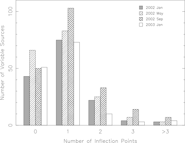
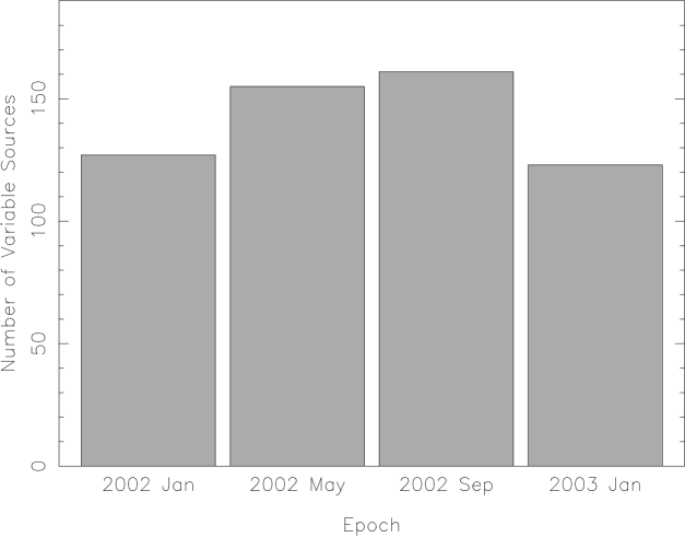
Figure 5: Upper: The number of sources classified as variable versus the observed number of changes in the sign of the derivative of flux density vs time (i.e. number of inflection points). Clearly a majority of the sources vary on timescales of 3 days or longer. Lower: Numbers of sources classified as variable in each epoch. Screens moving at the LSR would be expected to result in fewer variables beeing seen in epoch 3; we see no such deficit.

During the visual examination of the light curves for each source at each epoch, the timescales were estimated by counting the number of inflection points (i.e. change in sign of the derivative) for those epochs classified as variable. Since in the visual examination there was an effective smoothing, inflection points due to noise-like deviations were not counted. The majority of sources were found to show none or at most one inflection point indicating variability timescales that are predominantly longer than 3 days. The observed distribution of inflection points is shown in Figure 5. Only a small number of sources (20%) showed 2 or more inflection points. A comparison of the distribution of inflection points for the weak and strong sources revealed no significant difference between the two classes. Overall, the distribution of timescales was statistically the same for each epoch, remembering that epoch 3 was four days rather than the three days of the other epochs. An important conclusion from the timescale study is our 3 or 4 d lightcurves commonly underestimate both the timescale and true modulation index for many of the sources.

The annual cycle reported in a number of IDV sources is due to the changing relative velocities of the Earth and the ISM responsible for the scattering (Macquart & Jauncey, 2003). If the ISM velocities follow the Local Standard of Rest, many sources would be expected to exhibit slower variations in the third quarter of the year (i.e. during the third epoch), and hence may more easily be missed because of the lengthened time-scales. Figure 5 shows the numbers of variables found at each of the four epochs. A Chi-squared contingency test shows no evidence that the numbers differ from the mean in any epoch, even though epoch 3 lasted for four rather than three days. The uniformity of variable numbers in each epoch suggests a lack of evidence for a third-quarter slow-down, and it follows that the majority of the scattering material is not moving at the LSR. This is perhaps not unexpected; both PKS 1257–326 and J1819+3845, the two sources for which reliable screen velocities have been measured, have measured screen velocities that differ significantly from the LSR (Bignall et al., 2006; Dennett-Thorpe & de Bruyn, 2003; Linsky et al., 2007).

In summary we used the visual analysis to classify each source at each epoch as variable or not variable. We computed SFs for all sources and then examined the SFs of those classified as non-variable in order to quantify the measurement errors. We were able to correct the SFs by subtracting a constant versus time lag due to errors that are independent over the 2 h sampling and are characterized by equation 1. In addition we found a low level contaminating process with a timescale of 1-2 d, which we suggest is due to low-level confusion with an rms of 1-2 mJy. The SF of the slower contamination could not be reliably estimated and so sets a limit on the minimum detectable variation in flux density. By fitting a simple curve to the epoch-averaged and noise-corrected SFs, we estimated $D(t=2\,\mbox{d})$ for each source. The contamination is minimized by requiring this quantity to be above a threshold of $4\times 10^{-4}$ for a useable estimate of the timescale $\tau_{\rm char}$. Most sources were classified as slow variables.

4.4 Comparison of SF with the visual variability classification

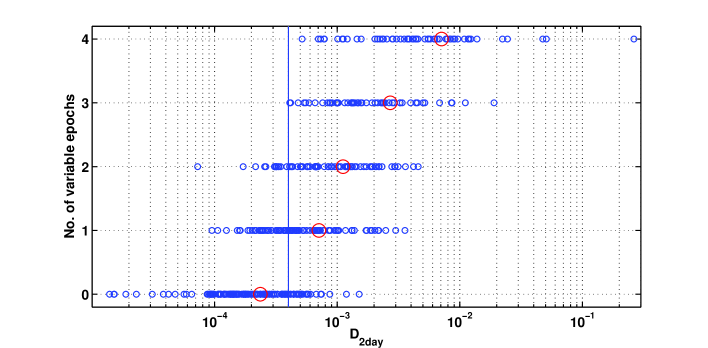
Figure 6: The number of “variable” epochs plotted against the value of $D(2\mbox{d})$ fitted to the cumulative structure function for all four epochs. The large circles show the mean values for each group of sources (see Table 3).

We now compare the SF analysis with the variability classification from §3. Figure 6 shows the number of epochs in which a source was classified as variable plotted against its value of $D(2\,\mbox{d})$ obtained as described from a fit to the structure function of the cumulative data from all 4 epochs. The large circle shows the mean values for each group of sources. While it is clear that the sources with higher $D(2\,\mbox{d})$ were classified as variable more frequently, there is a very wide distribution in the rms level of the variation over 2 d among the sources. The vertical line marks the threshold $D(2\,\mbox{d})=4\times 10^{-4}$ above which we have made a timescale estimate. Values below this should be regarded as upper bounds in view of the possibility of low level confusion.

Table 3 lists the source counts sorted by the number of “variable” epochs for the 443 sources (as always excluding those used as calibrators in more than one epoch.) It also shows the mean values of $D(2\,\mbox{d})$ and the numbers of sources above and below the SF threshold. In total 37% of them are above the threshold versus 45% from the variability classification on 2 or more epochs. In the latter classification process we do not characterize the rms amplitude but attempt to quantify any intermittency in the phenomenon. In contrast the SF analysis quantifies the rms amplitude over 2 d averaged over all 4 epochs.

5 Interpretation as Interstellar Scintillation

We now examine our basic hypothesis, stated in the introduction, that the variations in flux density detected in the MASIV survey are caused by interstellar scintillation (ISS). The extremely small diameters of pulsars revealed the ISS phenomenon almost as soon as pulsars were discovered and they still provide the best information on the distribution of small scale structure in the ionized interstellar medium – indeed they provide a calibration of the ISS phenomenon. The pulsar observations have been combined into a model for the distribution of electron density in the interstellar medium by Taylor & Cordes (1993) and revised by Cordes and Lazio (2005).

Because the refractive index of an ionized medium varies with radio frequency, there is a transition frequency ($f_{\rm w}$) above which the scintillation of a point source, like a pulsar, is weak in the sense that its scintillation (modulation) index ($m_{\rm pt}$) is less than one. This frequency is on the order of 5 GHz but depends on the strength of the turbulent fluctuations in electron density on the given line of sight (Walker, 1998; Cordes and Lazio, 2005). Above $f_{\rm w}$ the ISS of a point source has a single timescale approximately given by $t_{\rm F}=r_{\rm F}/V$, where $V$ is the effective velocity of the Earth through the ISS diffraction pattern and $r_{\rm F}=\sqrt{L\lambda/2\pi}$ and $L$ is the typical distance to the scattering region.

In our observations the angular diameters of the extra-galactic sources are considerably larger than those of pulsars and so their ISS is heavily quenched. See Rickett et al. (2006) for a discussion of how the “low-wavenumber approximation” can be applied for quenched scintillation even below the transition frequency. If we approximate the scattering as taking place in a thin region of the Galactic plane, we obtain simple expressions for the reduction in scintillation index and lengthening of timescale (e.g. Rickett (1986)). In Appendix A we apply the same simple “screen” model to the structure function analysis and obtain expressions for how the observable $D(2\,\mbox{d})$ might vary with angular size of each source and on distance to the scattering region and the level of turbulence on each line of sight. Of course the level of ISS also depends on properties of the source – in particular the fraction of its flux density in its most compact component and on the effective diameter of that component.

5.1 Galactic Dependence of ISS

We start by comparing our $D(2\mbox{d})$ results with the emission measure (column density of the square of the electron density) as estimated from observations of H$\alpha$ emission. We find the intensity of H$\alpha$ emission (in Rayleighs) from the WHAM Northern sky survey on a 1 degree grid (Haffner et al., 2003) nearest to each source. We use the intensity summed over all velocities, which Haffner et al. (2003) interpret as proportional to the ISM emission measure on that line of sight, assuming the temperature of the emitting gas does not vary by a large percentage. We expect the level of ISS to be related to the emission measure on that line of sight, as described by Spangler & Cordes (1998) and observed by Rickett et al. (2006).

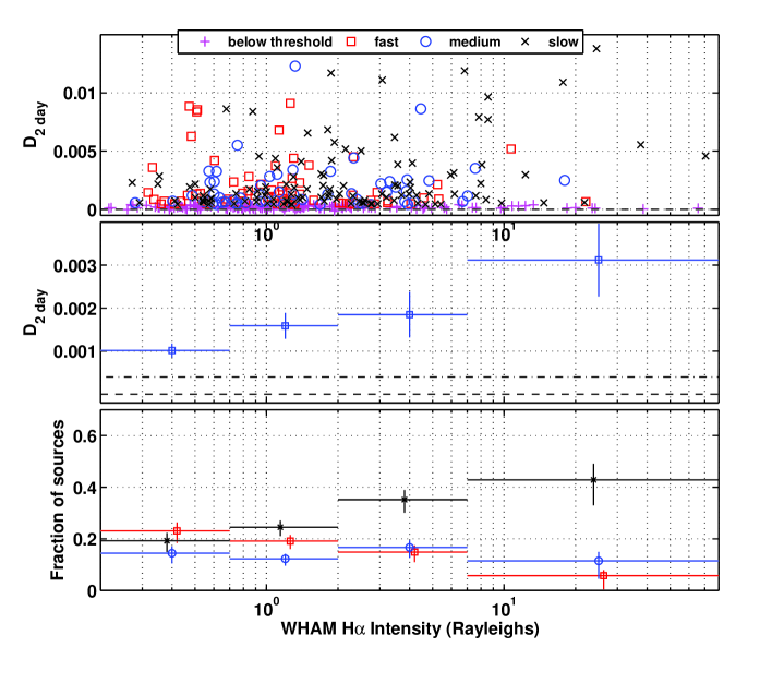
Figure 7: Upper panel: Log-log Scatter plot of $D(2\mbox{d})$ against WHAM H$\alpha$ emission which is proportional to the emission measure on a line of sight sampled on a 1 degree grid of the Northern sky (Haffner et al., 2003). The intra-hour variable source J1819+3845 is off scale at 0.25. The different symbols represent the three classifications of ISS timescale, as described in the text. Center panel: Mean value of $D(2\mbox{d})$ in the indicated bins of H$\alpha$ emission including all sources except J1819+3845; vertical bar gives the standard error in the mean. Lower panel: Fraction of sources above the threshold in each timescale class in each bin showing that fast ISS is commonest for the lower column density of electrons and slower ISS dominates for higher column densities. Error bars assume binomial distributions. The same method is used in Figures 8, 10, 11 & 13.

Figure 7 plots $D(2\mbox{d})$ against the WHAM H$\alpha$ emission (in Rayleighs). Though the scatter plot in the top panel shows little obvious trend, the bin averages in the middle panel show a clear upward trend with emission measure, which establishes ISS as the dominant cause of the variability in the MASIV survey. We stress the complete independence of the two data sets in this figure and that the bin averages are independent of any threshold set on $D(2\mbox{d})$. We exclude the extreme IHV source J1819+3845 from this and subsequent bin average plots because its $D(2\mbox{d})$ value is 0.25 which is so much higher than the next highest at 0.015 that it distorts the mean and the variance within its bin.

The bottom panel shows that the fraction of slowly scintillating sources clearly increases with emission measure and vice-versa for the fast scintillators. This finding that the longer timescales occur when seen through greater column density of electrons is consistent with enhanced ISS from strongly ionized regions of the ISM, which are typically at low Galactic latitudes and at greater distances $L$. An increase in $L$ increases the scale of the scintillation pattern which slows the scintillation time - see Appendix A.

Since the strength and effective distance of the scattering layer depends on Galactic latitude, we also expect a dependence of ISS on Galactic latitude. For our visual classification of sources (as variable or non-variable) we asked the simple question “are their latitude distributions the same?”. A Chi-squared contingency test dividing the sources into two samples, a low latitude sample, $|b|<$ 40 degrees, and high latitude sample, $|b|>$ 40 degrees, shows that the two distributions differ at the 98% confidence level. There are fractionally more variables at low latitudes than there are at high latitudes, supporting ISS as the origin of the intra-day variability.

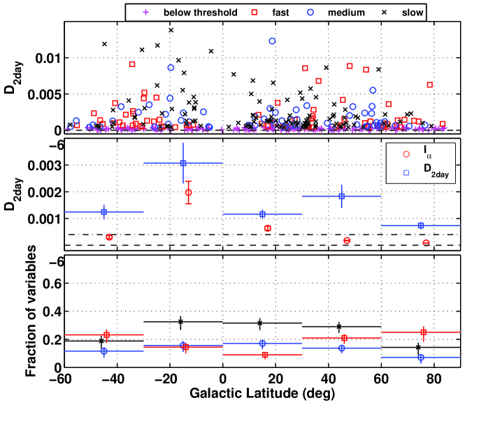
Figure 8: Upper panel: Scatter plot of $D(2\mbox{d})$ (on log scale) against Galactic latitude. The intra-hour variable source J1819+3845 is off scale at 0.25. The different symbols represent the three classifications of timescale, as described in §4.3. Center panel: Squares show mean value of $D(2\mbox{d})$ in 30 degree bins of latitude including all sources except J1819+3845; vertical bar gives the error in the mean. Note the N-S asymmetry in the circles show mean H$\alpha$ emission in each bin. Lower panel: Fraction of sources above the threshold in each timescale class in each bin.

For the structure function analysis we simply plot $D(2\mbox{d})$ against the Galactic latitude of each source, in a fashion similar to that of Heeschen & Rickett (1987). The upper panel of figure 8 is a scatter plot, differentiated by the timescale group (fast, medium or slow). The middle panel averages $D(2\mbox{d})$ into 30 degree wide bins for all sources, which as already noted is independent of the threshold on $D(2\mbox{d})$. There is a low level of scintillation above 60 degrees, increasing in the mid range (30-60 deg), in both northern and southern hemispheres. However in the low latitudes (0-30 deg) the ISS increases in the south of the plane but decreases north of the plane. While the figure is in reasonable agreement with the latitude dependence found by Rickett et al. (2006) in their analysis of the modulation index of 146 flat-spectrum sources observed at 2 GHz with the Green Bank Interferometer, there are competing effects in our MASIV survey since data were sampled for no more than 4 days.

As the latitude $b$ decreases both the distance $L$ to and the path length through the scattering medium increase ($\propto{\rm cosec}\;b)$. The increased path length makes the scintillation stronger at lower latitudes so that the modulation index should increase. However, the increased distance $L$ increases the scale of the scintillation pattern which slows the scintillation time so that the structure function will saturate at times longer than 4 days, causing a decrease in $D(2\mbox{d})$. The combination of these two effects requires careful modeling.

The model for the structure function described in Appendix A is a starting point for analyzing the effects of Galactic latitude. Equation (A5) shows that as the distance $L$ increases $D(2\mbox{d})$ should decrease. However, the equation assumes that the scintillation index of a point source $m_{\rm pt}=1$, omitting any increase due to the longer scattered path length at lower latitudes. In a more realistic model $m_{\rm pt}$ may be less than one looking out of the Galactic plane ($|b|\sim 90$ deg) and should increase with decreasing latitude, reaching unity at $\sim\pm 45$ deg (Walker, 1998). At lower latitudes still it will increase only slowly due to effects of refractive ISS. The increase in $m_{\rm pt}$ between 90 and 45 deg partially compensates for the reduction in $D(2\mbox{d})$ due to increasing distance $L$. At still lower latitudes $D(2\mbox{d})$ might be expected to decrease. In the observations one sees a difference of low latitude behavior between the Northern and Southern hemispheres. This asymmetry can be understood by looking at the center panel of Figure 8 which shows that the emission measure is commonly higher for Southern latitudes.

In a complete model the (unknown) compact fraction $f_{c}$ of the source flux density in the scintillating component must also be considered. Thus the expected variation of the ISS level with Galactic latitude must be combined with the probability distributions for the flux fraction and for the diameters of the compact components, which will further dilute the variation of $D(2\mbox{d})$ with latitude.

In the Green Bank Interferometer observations cited above, the data were sampled daily (or on alternate days) over many years and so provided estimates of the actual modulation index, which were not reduced by the lengthening ISS time scale at low latitudes. However, even for these data the latitude dependence is not a strong effect. Note that the asymmetry about the Galactic plane is very similar to the asymmetry in the typical H$\alpha$ emission as shown by the circles in the center plot. The lower panel of figure 8 plots the fraction of sources in the three timescale groups versus latitude and shows clear evidence that the fast scintillators dominate at high latitudes and that slow scintillators dominate at low latitudes. This agrees with the expected increase in ISS timescale at low latitudes outlined above.

5.2 Dependence of ISS on Source Spectral Index and Flux Density

As stated earlier the ISS of extragalactic sources is expected to be strongly suppressed, relative to that of pulsars, by the smoothing effect of their larger angular diameters. Consequently, we expect that the more compact sources should show higher levels of ISS. Here we examine the influence of mean flux density ($\bar{S}$) and spectral index $\alpha$ ($\bar{S}\propto\nu^{\alpha}$), since we expect synchrotron emitting sources to be more compact for larger $\alpha$ and lower $\bar{S}$, due to the effects of synchrotron self-absorption and inverse Compton losses.

In Heeschen (1984)’s initial survey of short-term variability of a large sample of both steep-spectrum and flat-spectrum sources he found that the flat-spectrum sources varied, “flicker”, but the steep-spectrum sources did not. This can be understood as the steep-spectrum sources are dominated by optically thin synchrotron emission with low brightness temperatures, while the flat spectrum sources are dominated by synchrotron self-absorbed components with very high brightness temperatures (Scheuer & Williams, 1968), making them compact enough to show ISS.

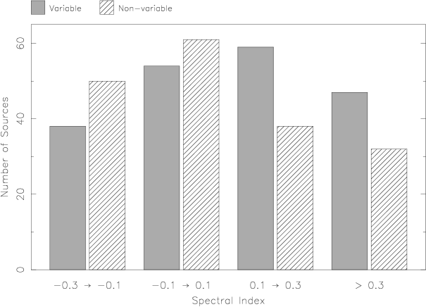
Figure 9: Number of variable and non-variable sources as a function of spectral index.

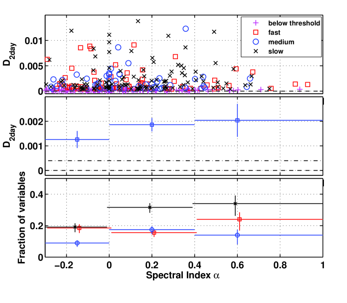
Figure 10: $D(2\mbox{d})$ as a function of spectral index. Upper panel: Logarithmic scatter plot of $D(2\mbox{d})$. Different symbols represent the three classifications of ISS timescale. Center panel: Mean $D(2\mbox{d})$ binned by spectral index including all sources except J1819+3845. Lower panel: Fraction of sources above the threshold in each timescale class in each bin. No significant trend is seen.

The MASIV sources were selected to have flat spectral indices $\alpha>-0.3$ (Lovell et al., 2003) and so are predominantly quasars with compact cores. However, it is possible that there are also some very compact galaxies in the sample. Figure 9 shows the spectral index distributions separately for the sources with the visual classification as variable or non-variable. The spectral indices shown are those used to form the sample: 1.4 GHz NVSS (Condon et al., 1998) to 8.5 GHz JVAS (Patnaik et al., 1992; Browne et al., 1998; Wilkinson et al., 1998) or CLASS (Myers et al., 1995) flux densities. This shows a slight increase in the fraction of sources that are variable with increasing $\alpha$, in agreement with the expectation that the flatter (and inverted) spectrum sources are more compact. Though in Figure 10 the mean $D(2\mbox{d})$ shows no significant trend with spectral index, the bottom panel shows a slight increase in the fraction of variable sources for $\alpha>0$. This is mostly due to an increase in the fraction of slow variables which constitute the largest timescale group. It is worth pointing out that the surveys from which the flux densities were drawn to obtain spectral index were not coeval. It is likely then that any change in sample properties as a function of spectral index will be blurred as many of the sources vary intrinsically.

Turning to the influence of mean flux density, we first discuss the visual variability classification and then plot $D(2\mbox{d})$ against flux density. The selection of sources for the MASIV survey divided them into a high mean flux density group (strong) and a low mean flux density group (weak $S<0.3$ Jy). As reported in Paper 1 there was a greater fraction of variable sources in epoch 1 from the low flux density group than from the high flux density group. Combining all four epochs the numbers of weak sources that varied in 0-4 epochs is (94, 46, 36, 39, 33) and for strong sources the numbers are (62, 45, 49, 22, 23). Thus there are significantly more 3 & 4 time variables among the weak sources than among the strong ones, though this trend is not supported in the 2 or 1 time variables.

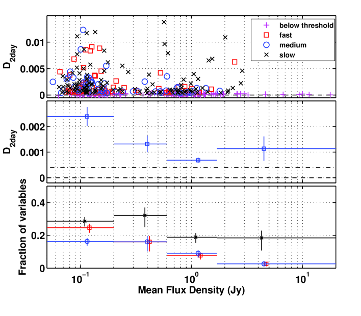
Figure 11: Upper panel: Scatter plot of $D(2\mbox{d})$ against mean flux density. The higher values are more common for lower flux density sources. The different symbols represent the three classifications of ISS timescale, as described in the text. Center panel: Mean value of $D(2\mbox{d})$ in bins of mean flux density for all sources (excluding extreme IHV quasar J1819+3845). Note lower levels of ISS for the sources with higher flux density. The points centered at 2.5 Jy have only a few sources in each timescale group giving larger errors in the mean for that bin. Lower panel: Fraction of sources in each timescale class in each bin. Note decreasing occurrence of fast variables among stronger sources.

Figure 11 shows $D(2\mbox{d})$ versus mean flux density. The center panel shows a clear downward trend with increasing flux density in the lowest three bins, while in the fourth bin it increases but with fewer sources the mean has a large error. The interpretation is an increasing angular diameter of the compact source components with increasing total mean flux density. Furthermore, the bottom panel shows a decrease in the fraction of fast and medium scintillators with increasing mean flux density. These are exactly the trends expected if their effective angular diameters are constrained by a maximum brightness temperature due to self-absorption or inverse Compton losses ($\theta\propto(\bar{S}/T_{\rm B})^{0.5}$).

5.3 Source Models

The foregoing analysis establishes that about half of the 443 compact flat spectrum radio sources in the MASIV survey show ISS at an rms level above 1% over times of 2 d. We now consider a simple model for the compact source structure based on Appendix A. Equation (A5) gives an approximate relation between $D(2\mbox{d})$ and parameters of the source ($f_{c}$ and $\theta_{\rm src}$) and of the interstellar medium ($L$ and $V$). We proceed by assuming a basic model for the latter parameters $L=500$ pc and $V=50$ km s^-1 and finding constraints on the source.

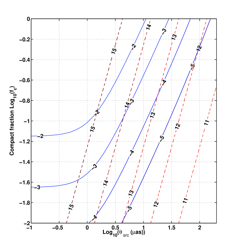
Figure 12: Solid lines show contours of $\log_{10}[D(2\mbox{d})]$ versus $f_{c}$ and $\theta_{\rm src}$ based on a Kolmogorov model for ISS in a region at a distance of 500 pc. Dashed lines are contours of $\log_{10}[T_{b}/\bar{S}_{\rm Jy}]$ for total source flux density $\bar{S}_{\rm Jy}$.

Figure 12 shows (solid) contours of $D(2\mbox{d})$ versus the source parameters: compact component diameter and compact flux fraction – defined in the observer’s frame. Also shown are (dashed) contours of $T_{b}/\bar{S}_{\rm Jy}$. The majority of sources are in the range $0.0004<D(2\mbox{d})<0.01$ which, for sources of 0.1 Jy mean flux density, maps to maximum brightness temperatures $10^{12}$K to $10^{14}$K. These figures require substantial Doppler factors in the AGN jets comparable with those estimated from VLBI. However, we note that the plot of Figure 12 only provides a guide since it is based on 500 pc as the distance to an interstellar scattering screen.

The distribution of scattering electrons along the line of sight to each source is likely to be much more complex and can extend from tens of pc to a few kpc. Scattering at tens of pc has been shown to be important for the rare rapid scintillators (IHV) and scattering from more than 1 kpc is responsible for the slower timescale ISS associated from sight lines with large emission measures. Since the implied angular diameters scale roughly with the distance, the uncertainty in $L$ corresponds to an extremely large range in implied brightness temperatures. We note, however, the fast ISS sources in our sample are mostly scintillating at levels of only 1-5%, unlike the large amplitude variations in the well studied IHV sources B0405–385, B1257–326 and J1819$+$3845. This suggests that the nearby scattering regions responsible are relatively rare covering only a small fraction of the sky. Lazio et al. (2008) discuss the relative importance of sparsely distributed “clumps of scattering material” and a more uniformly distributed interstellar scattering plasma, suggesting that the former could be more important for ISS and the latter for angular broadening in the ISM. These authors find minimum diameters of $\sim 1-2$ mas at 1 GHz, which they suggest is caused by interstellar scattering, which predicts $40-80\mu$as when scaled to 5 GHz. It will be important to use the full MASIV data set to re-examine these questions, but since our emphasis here is on presenting the data, we postpone them to a later paper.

5.4 Combined effects of Intrinsic Variations and ISS

Here we examine the competing contributions that scintillation and intrinsic variability would potentially make to the measured lightcurves. A source at an angular diameter distance $D_{A}$ undergoing intrinsic variations on a timescale $\tau$ has an implied maximum intrinsic angular size:

$$\theta=17.3\,{\cal D}\left(\frac{\tau}{100\,{\rm days}}\right)\left(\frac{D_{A}}{1\,{\rm Gpc}}\right)^{-1}\,\mu{\rm as},$$ (4)

where ${\cal D}$ is the Doppler factor. Further, a variation in flux density $\Delta S$ implies an observed brightness temperature of

$$T_{B}=6.4\times 10^{12}\,\left(\frac{\Delta S}{100\,{\rm mJy}}\right)\left(\frac{\tau}{100\,{\rm days}}\right)^{-2}\left(\frac{D_{A}}{1\,{\rm Gpc}}\right)^{2}\,{\rm K}.$$ (5)

When mapped into the emission rest frame the brightness temperature is then reduced by a factor ${\cal D}^{3}(1+z)^{-3}$, under the hypothesis of intrinsic variation.

As an example consider a source that undergoes $100\,$mJy intrinsic fluctuations in $100\,$days, as observed between epochs for several of our sources. At a typical distance $D_{A}\sim 1{\rm Gpc}$ the implied maximum source size would be $\sim 17\,{\cal D}\mu$as. Suppose further that it does not show ISS within an epoch, which implies it must be larger than $~{}80\,\mu$as in the observed frame and so ${\cal D}>4.6$. Hence mapping equation (5) into the emission frame gives $T_{\rm B,em}\mathbin{\lower 3.0pt\hbox{$\hbox to0.0pt{\raise 5.0pt\hbox{$\char 60\relax$}\hss}\mathchar 29208\relax$}}5\times 10^{10}$K. We conclude that sources showing intra-epoch (intrinsic) variation and no ISS have relatively low emission frame brightness and, conversely, higher brightness sources that show intra-epoch variation have to show ISS.

5.5 Dependence of ISS on Source Redshift

We found redshifts for about half of the 443 sources in the survey from the published literature and we have subsequently measured another 69 (Pursimo et al., 2008) for a total of 275 redshifts. This constitutes the largest sample of ISS measurements versus redshift.

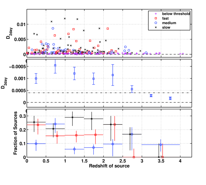
Figure 13: Upper panel: Scatter plot of $D(2\mbox{d})$ against source redshift. The different symbols represent the three classifications of ISS timescale, as described in the text. Center panel: Mean value of $D(2\mbox{d})$ in redshift bins for the 271 sources (out of 443) with measured redshift (excluding extreme IHV quasar J1819+3845). Note lower levels of ISS at high redshift. Values below the dash-dot line are upper bounds since they may be raised slightly by low level confusion. Lower panel: Fraction of sources in each timescale class in each bin. The two bins above z=3 have been combined, as there are so few sources at this redshift.

Figure 13 plots $D(2\mbox{d})$ versus redshift and reveals a highly significant decrease in the prevalence of ISS as redshift increases. In particular the middle panel shows that when binned in redshift the mean level of ISS drops steeply above redshift 2. As in other plots in this format the binned averages are independent of any SF threshold. However, note that the exact value of the lowest binned averages of $D(2\mbox{d})$ depend on the details of the noise subtraction. We note that, since the effect of confusion is to slightly increase $D(2\mbox{d})$, our estimates become upper limits when below the threshold of about 0.0004.

The bottom panel suggests that the fraction of fast variables drops more quickly with redshift than the fraction of slow and medium variables. However, the error bars show that this is only marginally significant, and in view of the importance of this question we list the source counts in Table 5. If true it would imply that the drop in mean ISS level is due to an increase in angular diameter with redshift, which also lengthens the ISS timescale. While the drop in ISS level seen in the middle panel could be due either to an increase in diameter of the compact core of emission from these sources or a decrease in the compact fraction of flux density in that core, the latter interpretation would not explain a steeper decrease in fast ISS with redshift than in slow ISS. The most likely conclusion from this analysis is that the extremely compact emitting regions responsible for the ISS in over half the quasars studied appear broader in angular diameter with redshift above 2. The interpretation of this result involves either an evolution in the emitting regions with redshift or an angular broadening phenomenon due to propagation. We caution that a full consideration of selection effects must be made when interpreting this result. For example, redshifts are currently more complete in the strong (84%) than the weak (43%) sub-samples. Therefore, although this new cosmologically important result is the major finding from the MASIV survey, we postpone a full discussion of the interpretation to a paper in preparation (Macquart et al., 2008) pending a thorough investigation of selection effects (Pursimo et al., 2008). Interested readers can consult preliminary discussions of the interpretation by Rickett et al. (2007). We also note that Lazio et al. (2008) plotted angular diameter at 1 GHz against redshift from a much smaller sample of scintillating and non-scintillating sources but could draw no firm conclusions.

5.6 Intermittent Variability

We now ask whether the sources that were only classified as variable in one to three of the four epochs are varying episodically or are the result of statistical uncertainty and a fixed threshold for variability on the raw modulation index. As a result of the measurement uncertainties there can be both false positives and false negatives, whose probabilities we can estimate. Concentrating on the 91 sources that were classified as variable in only one epoch and correcting for false positives leaves us with 61 sources $\sim 13$% of the total. These may be a category of short-lived, episodic scintillators revealed by our regular sampling over a full year.

We note the strong case for intermittent ISS in the rapid variable PKS 0405–385 (Kedziora-Chudczer et al., 2001b), and so consider a simple model for the intermittency in terms of the longevity of each IDV episode and the duration between episodes. Intermittency may arise either due to fluctuations in the level of turbulence responsible for ISS, or it may arise if the lifetimes of the bright, microarcsecond source components that undergo ISS are short. In the latter case one might expect sources to undergo IDV in conjunction with each outburst of the central engine.

Consider a simple model in which the IDV episodes have a finite duration $\Delta T$ and an interval, $T_{f}$, between outbursts. Obviously in reality both quantities will have a distribution of possible values, but given the infrequency of our time sampling we restrict ourselves to this simple assumption here. For any given source the IDV episode commences at some random time $t_{i}\in[0,T_{f})$, with the probability distribution of episodes distributed uniformly:

$$p(t_{i})=T_{f}^{-1},\quad 0\leq t_{i}<T_{f}.$$ (6)

If we make a single observation the probability that the source will be exhibiting IDV is

$$p_{1}=\Delta T/T_{f},$$ (7)

so for a survey that examines $N$ intermittent sources the expected number showing IDVs at any one time is $N\Delta T/T_{f}$. One can similarly calculate the probability of detecting IDV in a source during one or more of multiple observing epochs of a multi-epoch survey (see Appendix B). In particular, the probability of detecting IDV in a source in one or more epochs of a four epoch survey, with epochs separated evenly in time by $t_{\rm obs}$, is

$$p_{4}=\left\{\begin{array}[]{ll}\frac{\Delta T+3t_{\rm obs}}{T_{f}},&t_{\rm obs}\leq\Delta T,\\ \frac{4\Delta T}{T_{f}},&t_{\rm obs}>\Delta T.\\ \end{array}\right.$$ (10)

The number of IDV sources detected is a maximum when the interval between observing epochs exceeds the duration of IDV episodes because for shorter epoch intervals, after one merely discovers few new IDVs after the first epoch, one only keeps reobserving all the IDVs that were present in the first epoch. (Obviously, in the limit when $t_{\rm obs}$ is small, multiple observations discover the same number of sources as a single-epoch survey.)

Now, the mean detection rate of IDV sources in each epoch is 30%, whereas the fraction of sources that exhibited IDV in one or more of our four epochs is 58%. These two numbers imply a typical burst duration $\Delta T=1.2$ yr and a burst period of $T_{f}=3.8\,$yr.

We can also calculate the corresponding probability that IDV is observed in a source in all four epochs:

$$p_{\rm all4}=\left\{\begin{array}[]{ll}\frac{\Delta T-3t_{\rm obs}}{T_{f}},&3t_{\rm obs}<\Delta T,\\ 0,&3t_{\rm obs}>\Delta T.\end{array}\right.$$ (13)

Based on the foregoing estimates of $\Delta T$ and $T_{f}$ one estimates that only 4% of all sources should be common to all four epochs. However, the actual detection fraction is 12%.

It should be remembered that this model does not take into account several effects which are likely to be important, including: (i) annual cycle effects influence the number of sources one detects at any one epoch (ii) there is likely a distribution of episode durations and repetition rates, (iii) the repetition is likely irregular and (iv) not all IDVs are likely to be episodic. We favor (ii), the importance of which is illustrated by the fact that many one-time IDVs were seen in epochs 2 & 3 that were (obviously) not detected in epoch 4. However, our model implies that sources that commenced IDV in these epochs should have been detected subsequently because the predicted burst duration exceeds the interval between observing runs (i.e. $\Delta T>3t_{\rm obs}$).

6 Conclusions

We have reported results from the four epochs of the MASIV survey. There were 710 sources with flat spectra ($\alpha<-0.3$) near 5 GHz selected in weak and strong flux density groups surveyed for variability in four epochs over a year. These flat spectrum sources are predominantly quasars with compact emission probably from a core and jet, many with effective diameters small enough to show interstellar scintillation (ISS). In each epoch the flux density was measured using sub-arrays of the VLA every 2 hrs for about 12 hrs each day for 3-4 days. Sources were removed from the study if they showed evidence for changing correlated flux density due to confusion or resolution of their more extended structure, leaving 443 sources which were analyzed for variability in two ways.

The first was a binary classification based on the raw modulation index (visual method) in which 43% of the sources were classified as variable in 2, 3 or 4 of the epochs. The second was a fit to the epoch-averaged structure function parameterized by $D(2\mbox{d})$ and a timescale $\tau_{\rm char}$. In view of the uncertainties in the latter we classified sources as slow ($>3$ days), medium (0.5-3 days) or fast ($<0.5$ days) if $D(2\mbox{d})$ exceeded $4\times 10^{-4}$. By this criterion 37% of the sources varied with more than 1.4% modulation index over 2 days, which is similar to the 43% variables by the visual classification.

We found that $D(2\mbox{d})$ and timescale varied both with coordinates in the Galaxy and also with source-based quantities. This confirms that the variations are dominated by ISS, which depends on both the strength of scattering and the distance to the scattering region and also on the fraction of flux density in its most compact component and its effective angular diameter. The following is a summary of our findings:

• The amplitude of 2-d variability increases with increasing emission measure estimated from H$\alpha$ intensity for each line of sight. Emission measure is the column density for the square of the electron density which is expected to be strongly correlated with inhomogeneity in the ionized medium that causes ISS. This result provides observational evidence that ISS is the dominant cause of the variations. We find fast variations dominate for low emission measure, as expected since such regions will be seen out of the plane and closer to the Earth, and slow variations dominate for high emission measure which are typically seen at greater distances toward the Galactic plane especially for southern latitudes where the H$\alpha$ intensity is high.

• The amplitude of 2-d ISS variability varies significantly with Galactic latitude but differs substantially between positive and negative latitudes. The expected behaviour is complicated; greater path lengths at low latitudes, where the scattering should be stronger, cause the scattering to be slower which should reduce the rms over 3 d. However, the observed timescales show that there are more sources with fast variations at high latitudes and more sources with slow variations at low latitudes in both hemispheres, in clear support of ISS as the dominant cause.

• The ISS modulation index tends to decrease with increasing mean flux density, as expected if the compact emission is limited by synchrotron self absorption or inverse Compton losses to have a maximum brightness temperature. In that case the expected angular diameter $\propto\sqrt{\bar{S}}$ which will quench the ISS of the stronger sources.

• There is little change in the ISS amplitude with spectral index for our sample with $\alpha>-0.3$.

• There is evidence that the ISS can be intermittent on times of 3-6 months for some sources, but this is hard to quantify from the 3 day observing sequences, when the time scale of the variations is of the same order.

• We model $D(2\mbox{d})$ as a function of compact source component fractional flux density and angular diameter, from which we find compact diameter to lie in the range 0.005 – 0.15 milli arcseconds and brightness temperatures in the range $10^{12}-10^{14}$K.

• The most far-reaching result reported here is the discovery of a decrease in both the fraction of sources that scintillate and in their scintillation amplitude beyond redshifts around 2. We conclude that there is an increase in the typical angular diameter of the most compact radio-emitting regions of the quasars beyond reshift 2. The possible interpretations of this exciting result will be presented in a companion paper (Macquart et al., 2008).

• A further surprise (at least to us) was the apparent absence of the very rapid variables (IHV). J1819+3845 fell in our sample, but it was the only source to show remarkable large amplitude variability. J0929+5013 showed rapid variability in the January 2002 epoch (Lovell et al., 2003) but, although monitored closely, revealed only slower, many-hour variability in the three later epochs. We had expected to find more of these rapid variables especially given that two of the three known, J1819+3845 and PKS1257-326 were discovered serendipitously. This strongly suggests that the IHV sources lie behind discrete local interstellar clouds which cover a small fraction of the sky.

Appendix A Structure function for ISS

In all of the MASIV data the intrinsic source diameters ($\theta_{\rm src}$) are large enough to suppress the scintillations relative to those of a point source (such as a pulsar), which at 6 cm would be expected to have a true modulation index $m_{\rm pt}$ near unity. In this section we describe a model for the structure function for such extended sources; this is easier to interpret than the apparent modulation index $m_{i}$.

The source diameter smoothes the ISS of a point source and so reduces the modulation index to $m_{\theta}$ and lengthens the timescale to $\tau_{\theta}$. If the scattering is concentrated at a distance $L$ from the Earth and we are near the transition from weak to strong scintillation, a useful approximate relation is:

$$m_{\theta}\sim m_{\rm pt}\frac{\theta_{\rm F}^{7/6}}{(\theta_{\rm F}^{2}+\theta_{\rm src}^{2})^{7/12}}\,.$$ (A1)

Here $\theta_{\rm F}=\sqrt{\lambda/(2\pi L)}$ is the angular size subtended by the Fresnel scale ($r_{\rm F}$) and $\theta_{\rm src}$ is the angular radius of the source. The exponents $7/6$ and $7/12$ apply for a Kolmogorov spectrum of interstellar turbulence (Coles et al., 1987). To the same accuracy the ISS timescale for a point source would be $\tau_{\rm F}=L\theta_{\rm F}/V$ and the source smoothing would increase it to:

$$\tau_{\theta}=\tau_{\rm F}\frac{\sqrt{\theta_{\rm F}^{2}+\theta_{\rm src}^{2}}}{\theta_{\rm F}}\,,$$ (A2)

where $V$ is the effective transverse velocity of the observer relative to the layer of scattering plasma. Note that when the source diameter is sufficiently large to suppress the scintillations we have

$$m_{\theta}\sim(\theta_{\rm F}/\theta_{\rm src})^{7/6}\;,\tau_{\theta}\sim L\theta_{\rm src}/V\,,$$ (A3)

where we have set $m_{\rm pt}=1$ (Rickett, 1986).

The theoretical form of the auto-correlation function for an extended source that substantially suppresses the scintillation index is given by the low wavenumber approximation of Coles et al. (1987). This in turn gives the theoretical structure function, whose detailed shape depends on both the spectrum of the plasma density and on its distribution along the line of sight through the Galaxy. Figure 14 of Rickett et al. (2006) shows the form for sources with Gaussian brightness with peak temperature $10^{11}-10^{13}$K, when the medium is modeled by the Cordes and Lazio (2005) electron distribution at a Galactic latitude of 45^∘ (away from the Galactic center). The form of the structure function at small time lags depends strongly on the density distribution in the local ISM. A useful approximation to these results is given by:

$$D(t)=2f_{c}^{2}m_{\theta}^{2}\frac{t^{a}}{t^{a}+\tau_{\theta}^{a}}\,,$$ (A4)

where $1\leq a\leq 2$ is a constant that depends on the density distribution in the local ISM. Here $a\sim 2$ for a local bubble with low turbulence such that the effective scattering distance is beyond the bubble ($>100$ pc) and alternatively $a\sim 1$ if the medium is uniformly turbulent out to a scale height (as in the “disk” of the CL05 electron density model). We have also introduced an extra variable $f_{c}$ that is the fraction of the source flux density in the bright (core) component.

Equations (A4) and (A3) thus provide a simple interpretation for our estimates of $D(t=2\mbox{d})$. Inserting $m_{\theta}$ and $\tau_{\theta}$ from equation (A3) we obtain:

$$D(2\mbox{d})=2f_{c}^{2}[\frac{1}{1+2\pi L\theta_{\rm src}^{2}/\lambda}]^{7/6}\frac{1}{1+(L\theta_{\rm src}/V2\mbox{d})^{a}}\,,$$ (A5)

An important feature of this result is that $D(2\mbox{d})$ decreases steeply with increasing $\theta_{\rm src}$ and so provides a sensitive measure of source diameter. In estimating $D(2\mbox{d})$ for every source-epoch we set $a=1$, which allows us to estimate the scintillation timescale $\tau_{\theta}$ without having to also estimate the exponent $a$. $D(2\mbox{d})$ can be converted to an effective 2-day modulation index by $m_{2\rm{d}}=\sqrt{0.5D(2\mbox{d})}$. We note that $m_{2\rm{d}}$ can substantially exceed the apparent modulation index $m_{i}$ when the time scale is longer than about 2 days.

Appendix B A simple model for IDV intermittency

Consider a model in which a source outbursts every duration $T_{f}$ in time and each IDV episode lasts $\Delta T$. The initial outburst time is unknown, but its probability is evenly distributed in the interval $t_{i}\in[0,T_{f})$: $p(t_{i})=T_{f}^{-1}$. Now consider a function $\bar{f}(t)=1-[H(t)-H(t-\Delta T)]$, which assumes the value one whenever the source shows no IDV but the value zero when it is on.

Thus the fraction of the time in which the source is off for initial burst durations between $t_{i}$ and $t_{i}+d\delta t_{i}$ is $\bar{f}(t_{i})p(t_{i})\delta t_{i}$. Thus the probability that IDV is absent is

$$p_{\rm 1off} = \int_{0}^{T_{f}}dt_{i}\bar{f}(t_{i})p(t_{i})$$ (B1)

$$= 1-\frac{\Delta T}{T_{f}}.$$

Thus the probability that the source is observed to exhibit IDV is $1-p_{\rm 1off}=\Delta T/T_{f}$.

Now suppose we look for IDV at times $t=0,t_{\rm obs},2t_{\rm obs},3t_{\rm obs}$. The fraction of the burst times between $t_{i}$ and $t_{i}+\delta t_{i}$ for which IDV is absent in all four observations is $\bar{f}(t_{i})\bar{f}(t_{i}+t_{\rm obs})\bar{f}(t_{i}+2t_{\rm obs})\bar{f}(t_{i}+3t_{\rm obs})p(t_{i})\delta t_{i}$. If we assume that the repetition period exceeds the total duration of our observations (i.e. $T_{f}>3\,t_{\rm obs}$), the probability of observing no IDV over all four epochs is

$$p_{\rm 4off} = \int_{0}^{T_{f}}dt_{i}\bar{f}(t_{i})\bar{f}(t_{i}+t_{\rm obs})\bar{f}(t_{i}+2t_{\rm obs})\bar{f}(t_{i}+3t_{\rm obs})p(t_{i})$$ (B4)

$$= \left\{\begin{array}[]{ll}1-\frac{\Delta T+3t_{\rm obs}}{T_{f}},&t_{\rm obs}\leq\Delta T,\\ 1-\frac{4\Delta T}{T_{f}},&t_{\rm obs}>\Delta T.\end{array}\right.$$

Thus the probability that IDV is observed in any one or more of these four epochs is

$$p_{\hbox{\footnotesize any of 4 on}}=1-p_{\rm 4off}=\left\{\begin{array}[]{ll}\frac{\Delta T+3t_{\rm obs}}{T_{f}},&t_{\rm obs}\leq\Delta T,\\ \frac{4\Delta T}{T_{f}},&t_{\rm obs}>\Delta T.\end{array}\right.$$ (B7)

We can similarly consider the probability of observing IDV in multiple observations by defining the function $f(t)=H(t)-H(t-\Delta T)$ which takes the value one whenever the IDV is on and zero otherwise. The probability that IDV is observed in all four epochs is thus

$$p_{\rm 4on} = \int_{0}^{T_{f}}dt_{i}f(t_{i})f(t_{i}+t_{\rm obs})f(t_{i}+2t_{\rm obs})f(t_{i}+3t_{\rm obs})p(t_{i})$$ (B10)

$$= \left\{\begin{array}[]{ll}\frac{\Delta T-3t_{\rm obs}}{T_{f}},&3t_{\rm obs}\leq\Delta T,\\ 0,&T_{f}>3t_{\rm obs}>\Delta T.\end{array}\right.$$

Table 1: A Summary of the observation dates, durations and VLA array configurations for the first four MASIV epochs.

Epoch Number	Start Time (UT)		Duration (h)	Array Configuration
1	2002 January 19,	19:14	72	D $\rightarrow$ A
2	2002 May 9,	08:02	72	A $\rightarrow$ BnA
3	2002 September 13,	17:50	96	B $\rightarrow$ CnB
4	2003 January 10,	16:21	72	C $\rightarrow$ DnC

Table 2: Observed numbers and percentages of sources classified as variable in the four epochs. Percentages are given of the 443 sources observed, which excludes those used as calibrators in more than one epoch. The predicted percentage of misclassifications assuming all sources were non-variable (where $P=0.05$ is the probability of a single misclassification).

Number of	Observed number	Observed percentage	Predicted fraction	Predicted fraction
variable epochs	of sources	of sources	of misclassifications	if none are variable
0	161	36%	$(1-P)^{4}$	81.5%
1	90	21%	$4P(1-P)^{3}$	17.2%
2	79	18%	$6P^{2}(1-P)^{2}$	1.3%
3	58	13%	$4P^{3}(1-P)$	0.05%
4	55	12%	$P^{4}$	0.0006%

Table 3: Statistics of SF and visual variability classifications for the 443 source sample.

No. epochs “variable”	No. of Sources	% Sources	Mean $D(2\,\mbox{d})$	No. $>4\times 10^{-4}$	No. $<4\times 10^{-4}$
0	161	36%	0.00024	27	134
1	90	21%	0.00071	54	36
2	79	18%	0.0011	64	15
3	58	13%	0.0027	58	0
4	55	12%	0.0071	55	0

Table 4: MASIV source variability characteristics. Column 4 gives H$\alpha$ in Rayleighs for WHAM. Columns 5-8 give mean flux density for epochs 1-4; Columns 9-12 give raw modulation index in % for epochs 1-4; Column 13 $\sigma_{\rm err}$ as %; Column 14 gives the visual classification per epoch for variable (y), non-variable (n) and non-variable source used as a secondary calibrator (c); Column 15 gives $D(2{\rm d})$ from fit to epoch average SF where error -1 flags a non-convergent fit; Column 16 gives timescale classifications, 1:$\tau_{\rm char}<0.5$d, 2:0.5d$<\tau_{\rm char}<3$d, 3:$\tau_{\rm char}>3$d, 0: $D(2{\rm d})$ below threshold of $4\times 10^{-4}$.

Name	RA(J2000)	Dec(J2000)	H$\alpha$ R	$\bar{S_{\nu}}$(Jy)	Mod index %	%err	Var	$D(2{\rm d})$	tim
J0005+3820	00:05:57.17	38:20:15.1	2.9	0.61 0.57 0.43 0.47	1.1 1.1 1.2 1.5	0.57	nnny	+4.73e-04 $\pm$ 1.4e-05	3
J0007+5706	00:07:48.47	57:06:10.4	10.8	0.18 0.20 0.17 0.17	2.1 0.9 1.1 1.0	0.88	nnnn	+2.91e-04 $\pm$ 4.3e-05	0
J0009+1513	00:09:43.47	15:13:37.9	0.7	0.16 0.16 0.17 0.16	1.0 1.7 2.0 1.3	0.94	nnnn	+4.92e-04 $\pm$ 5.5e-05	2
J0010+1724	00:10:33.99	17:24:18.7	0.8	0.85 0.83 0.81 0.81	0.8 1.0 0.9 0.5	0.53	nnnn	+1.07e-04 $\pm$ 1.3e-05	0
J0010+4412	00:10:30.04	44:12:42.4	2.3	0.20 0.20 0.19 0.18	1.5 1.2 1.5 1.7	0.83	nynn	+4.28e-04 $\pm$ 3.9e-05	1
J0011+7045	00:11:31.90	70:45:31.6	6.7	0.62 0.71 0.63 0.59	1.9 0.6 0.6 1.4	0.54	ynny	+3.46e-04 $\pm$ 3.6e-05	0
J0017+5312	00:17:51.75	53:12:19.1	13.3	0.61 0.60 0.61 0.65	1.5 0.9 1.2 1.2	0.54	nnyy	+3.88e-04 $\pm$ -1.0e+00	0
J0017+8135	00:17:08.47	81:35:08.1	2.2	0.91 0.92 0.92 0.92	1.4 1.2 0.5 0.7	0.52	nnnn	+2.13e-04 $\pm$ 1.6e-05	0
J0019+2021	00:19:37.85	20:21:45.5	0.7	1.16 1.05 1.03 1.22	2.0 0.2 1.0 0.7	0.52	ynnn	+4.86e-04 $\pm$ 3.6e-05	3
J0019+7327	00:19:45.78	73:27:30.0	4.3	0.45 0.46 0.47 0.47	1.5 0.8 1.7 1.0	0.57	nnyn	+5.27e-04 $\pm$ 1.0e+03	3
J0038+4137	00:38:24.84	41:37:06.0	2.6	0.53 0.53 0.53 0.53	1.3 0.9 1.6 1.0	0.56	ynyn	+5.71e-04 $\pm$ 2.6e-05	3
J0041+1339	00:41:17.21	13:39:27.4	1.1	0.15 0.16 0.16 0.16	0.8 2.5 1.9 1.8	0.97	nynn	+7.29e-04 $\pm$ 5.7e-05	2
J0042+2320	00:42:04.54	23:20:01.1	0.7	0.78 0.79 0.84 0.87	0.7 1.0 0.8 0.1	0.52	nnnn	+1.87e-04 $\pm$ 1.0e+03	0
J0042+5708	00:42:19.45	57:08:36.5	23.5	0.86 0.84 0.86 0.83	1.4 0.9 0.4 0.5	0.52	ynnn	+1.06e-04 $\pm$ 9.5e-06	0
J0043+0502	00:43:46.73	05:02:56.0	0.4	0.10 0.10 0.10 0.10	1.1 2.3 2.2 1.8	1.40	nnnn	+7.44e-04 $\pm$ 8.5e-05	3
J0052+1633	00:52:36.16	16:33:00.4	0.8	0.17 0.17 0.17 0.17	0.8 1.0 1.1 0.4	0.91	nnnn	+1.39e-05 $\pm$ 1.0e+03	0
J0056+1625	00:56:55.29	16:25:13.3	0.8	0.19 0.23 0.29 0.27	1.7 3.0 2.9 1.8	0.72	nyyy	+1.39e-03 $\pm$ 1.1e-04	1
J0056+3142	00:56:22.61	31:42:09.1	1.2	0.08 0.08 0.07 0.07	2.3 2.2 2.2 2.6	1.82	nnnn	+5.83e-04 $\pm$ 9.3e-05	1
J0057+3021	00:57:48.88	30:21:08.8	1.2	0.67 0.69 0.70 0.67	0.6 1.0 1.3 1.2	0.53	nnnn	+2.36e-04 $\pm$ 2.4e-05	0
J0101+5004	01:01:16.99	50:04:44.9	7.0	0.16 0.16 0.17 0.16	2.6 1.1 1.7 2.9	0.95	ynny	+1.16e-03 $\pm$ 1.1e-04	2
J0102+5824	01:02:45.76	58:24:11.1	17.7	1.37 1.88 2.63 2.34	8.0 3.5 6.3 3.1	0.53	yyyy	+1.09e-02 $\pm$ 3.4e-04	3
J0104+1134	01:04:10.62	11:34:16.3	0.8	0.08 0.08 0.08 0.08	1.4 2.5 1.8 1.7	1.70	nnnn	+3.64e-04 $\pm$ 8.5e-05	0
J0104+2949	01:04:08.32	29:49:05.6	1.2	0.09 0.09 0.09 0.09	2.8 3.5 2.2 1.5	1.54	yynn	+9.06e-04 $\pm$ 1.4e-04	1
J0105+4819	01:05:49.92	48:19:03.1	5.4	1.09 1.17 1.15 1.19	0.8 0.2 1.0 0.2	0.51	nnnn	+1.87e-04 $\pm$ 2.2e-05	0
J0108+0135	01:08:38.77	01:35:00.3	0.7	2.41 2.41 2.60 2.83	0.5 1.7 1.3 0.8	0.50	nyyn	+2.56e-04 $\pm$ 3.6e-05	0
J0111+3906	01:11:37.31	39:06:28.0	1.8	1.31 1.34 1.29 1.31	0.2 0.6 0.7 0.7	0.51	nnnn	+4.77e-05 $\pm$ 6.6e-06	0
J0121+0422	01:21:56.86	04:22:24.7	0.6	0.89 0.89 0.95 0.97	1.6 2.0 1.2 0.7	0.52	yynn	+5.13e-04 $\pm$ 2.9e-05	2
J0121+1149	01:21:41.59	11:49:50.4	0.7	1.70 1.71 1.57 1.59	0.7 1.4 0.5 0.8	0.51	nnnn	+1.34e-04 $\pm$ 1.8e-05	0
J0122+0310	01:22:01.91	03:10:02.4	0.5	0.12 0.11 0.10 0.10	0.7 1.6 1.6 1.4	1.30	nnnn	+1.30e-04 $\pm$ 5.1e-05	0
J0122+2502	01:22:38.81	25:02:31.7	0.9	0.82 0.82 0.84 0.86	1.1 1.5 1.1 1.2	0.52	nnny	+3.81e-04 $\pm$ 2.5e-05	0
J0122+2536	01:22:40.77	25:36:14.9	0.9	0.10 0.11 0.11 0.12	1.5 2.0 1.8 4.8	1.27	nnny	+2.16e-03 $\pm$ 3.9e-04	1
J0126+2559	01:26:42.79	25:59:01.2	1.0	0.74 0.76 0.79 0.81	0.8 2.1 0.8 0.5	0.53	nynn	+3.68e-04 $\pm$ 6.2e-05	0
J0135+2158	01:35:53.49	21:58:16.1	0.9	0.13 0.13 0.12 0.12	1.5 1.6 1.5 1.1	1.15	nnnn	+3.04e-04 $\pm$ 2.7e-05	0
J0136+4751	01:36:58.59	47:51:29.1	8.0	2.75 3.26 2.52 2.71	1.8 2.0 1.2 4.2	0.51	yyyy	+2.23e-03 $\pm$ 6.4e-05	3
J0141+7506	01:41:00.62	75:06:28.2	1.9	0.09 0.10 0.09 0.09	4.3 1.4 2.1 2.0	1.49	ynnn	+1.72e-03 $\pm$ -1.0e+00	3
J0150+2646	01:50:02.80	26:46:28.0	1.3	0.12 0.14 0.13 0.12	7.7 4.2 4.2 7.2	1.14	yyyy	+9.10e-03 $\pm$ 1.9e-03	1
J0151+2744	01:51:27.14	27:44:41.7	1.4	0.85 0.84 0.83 0.83	0.2 0.8 0.8 0.4	0.52	nnnn	+9.88e-05 $\pm$ 2.0e-05	0
J0152+2207	01:52:18.05	22:07:07.7	0.9	1.06 1.04 1.04 1.06	1.2 1.0 0.7 0.6	0.52	ynnn	+1.25e-04 $\pm$ 1.5e-05	0
J0154+4743	01:54:56.29	47:43:26.5	8.4	0.44 0.35 0.39 0.39	1.3 1.0 2.0 2.0	0.60	ynyy	+8.34e-04 $\pm$ 4.9e-05	3
J0158+4137	01:58:23.84	41:37:39.5	2.6	0.08 0.08 0.08 0.09	1.9 1.6 1.4 2.0	1.63	nnnn	+1.11e-04 $\pm$ 3.4e-05	0
J0200+0322	02:00:40.81	03:22:49.5	0.5	0.32 0.27 0.22 0.20	1.0 2.8 1.2 0.9	0.75	nynn	+6.87e-04 $\pm$ 8.3e-05	1
J0204+1514	02:04:50.41	15:14:11.0	0.7	2.81 3.07 3.04 3.01	0.9 1.3 0.1 0.8	0.50	nnnn	+2.38e-04 $\pm$ 2.9e-05	0
J0212+3626	02:12:09.73	36:26:17.9	2.2	0.09 0.08 0.08 0.08	2.3 1.8 1.4 2.1	1.68	nnnn	+3.78e-04 $\pm$ 9.3e-05	0
J0213+3652	02:13:48.19	36:52:33.9	2.1	0.13 0.16 0.16 0.18	1.6 1.2 2.0 1.0	0.96	nnyn	+5.35e-04 $\pm$ 1.0e+03	1
J0217+7349	02:17:30.81	73:49:32.6	2.2	3.43 3.46 3.41 3.41	0.1 1.0 0.1 0.1	0.50	nnnn	+3.95e-04 $\pm$ 2.7e-05	0
J0228+6721	02:28:50.05	67:21:03.0	4.3	2.07 2.02 1.79 1.63	0.6 0.1 0.6 0.3	0.51	nnnn	+2.30e-05 $\pm$ 4.7e-06	0
J0237+2046	02:37:50.62	20:46:18.4	1.4	0.10 0.10 0.10 0.10	3.5 5.2 2.8 2.4	1.41	yyyy	+4.10e-03 $\pm$ 2.3e-04	3
J0237+2848	02:37:52.40	28:48:08.9	1.8	2.78 3.05 3.47 3.69	0.9 0.4 1.1 0.1	0.50	nnnn	+3.08e-04 $\pm$ 5.5e-05	0
J0238+1636	02:38:38.93	16:36:59.2	1.1	1.50 1.61 1.58 1.34	2.8 3.0 1.2 1.8	0.51	yyyy	+1.19e-03 $\pm$ 9.5e-05	1
J0239+0416	02:39:51.26	04:16:21.4	0.8	0.65 0.60 0.60 0.68	0.7 0.9 1.6 0.5	0.54	nnnn	+3.06e-04 $\pm$ 4.5e-05	0
J0242+1101	02:42:29.17	11:01:00.7	1.0	1.12 1.16 1.24 1.21	0.2 1.1 0.9 0.8	0.51	nnnn	+1.41e-04 $\pm$ 2.2e-05	0
J0246+3536	02:46:21.07	35:36:37.9	3.0	0.17 0.17 0.16 0.16	1.6 4.1 2.1 1.1	0.93	nyyn	+2.20e-03 $\pm$ 1.5e-04	2
J0248+0434	02:48:14.82	04:34:40.8	0.8	0.15 0.15 0.15 0.14	0.9 1.0 1.1 1.3	1.01	nnnn	+4.21e-05 $\pm$ 1.8e-05	0
J0249+0619	02:49:18.01	06:19:51.9	0.8	0.68 0.68 0.70 0.68	0.9 1.1 1.1 0.9	0.53	nnnn	+1.75e-04 $\pm$ 2.3e-05	0
J0251+4315	02:51:34.53	43:15:15.8	5.7	1.18 1.23 1.20 1.21	0.6 0.6 0.2 0.2	0.51	nnnn	+6.50e-06 $\pm$ 4.1e-06	0
J0253+3217	02:53:33.65	32:17:20.8	2.7	0.09 0.11 0.12 0.14	2.5 12.5 6.6 4.3	1.21	yyyy	+2.23e-02 $\pm$ 1.5e-03	3
J0257+4338	02:57:59.07	43:38:37.6	5.6	0.13 0.14 0.14 0.14	1.5 0.8 1.4 1.2	1.07	nnnn	+2.11e-04 $\pm$ 2.4e-05	0
J0259+1925	02:59:29.65	19:25:44.3	1.3	0.20 0.23 0.22 0.19	1.6 4.8 2.4 3.1	0.80	nyyy	+2.65e-03 $\pm$ 2.6e-04	1
J0301+0221	03:01:00.08	02:21:46.4	2.3	0.14 0.13 0.14 0.13	1.2 1.4 1.4 1.0	1.09	nnnn	+8.83e-05 $\pm$ 2.1e-05	0
J0303+4716	03:03:35.24	47:16:16.2	5.0	1.28 1.29 1.41 1.22	0.4 1.1 0.5 0.4	0.51	nnnn	+1.12e-04 $\pm$ 9.2e-06	0
J0304+6821	03:04:22.00	68:21:37.4	2.6	0.65 0.67 0.68 0.67	1.8 1.4 0.7 0.7	0.54	yynn	+3.29e-04 $\pm$ 3.7e-05	0
J0308+1208	03:08:39.38	12:08:49.7	1.9	0.08 0.08 0.08 0.07	4.5 3.7 4.0 1.2	1.76	yyyn	+3.26e-03 $\pm$ 2.1e-04	2
J0309+1029	03:09:03.62	10:29:16.3	1.5	0.65 0.69 0.73 0.71	0.7 1.2 1.2 0.5	0.53	nnnn	+3.51e-04 $\pm$ 2.2e-05	0
J0313+0228	03:13:13.40	02:28:35.2	6.8	0.13 0.13 0.15 0.13	6.3 6.9 6.7 3.0	1.07	yyyy	+1.19e-02 $\pm$ 5.9e-04	3
J0314+4345	03:14:08.05	43:45:19.7	3.5	0.20 0.21 0.20 0.20	1.1 1.1 1.1 0.7	0.81	nnnn	+1.35e-04 $\pm$ 2.5e-05	0
J0319+4130	03:19:48.16	41:30:42.1	4.6	18.10 18.10 17.40 17.30	0.5 0.5 0.7 0.1	0.50	nnnn	+3.82e-05 $\pm$ 7.9e-06	0
J0321+1221	03:21:53.10	12:21:13.9	2.1	1.50 1.52 1.51 1.49	0.7 1.6 1.0 0.8	0.51	nnnn	+2.36e-04 $\pm$ 3.0e-05	0
J0323+0446	03:23:14.72	04:46:12.5	4.6	0.15 0.15 0.14 0.13	2.3 3.1 1.4 2.8	1.04	yyny	+9.87e-04 $\pm$ 1.7e-04	1
J0328+2552	03:28:44.34	25:52:08.4	3.5	0.16 0.17 0.19 0.17	1.8 3.5 5.0 1.5	0.89	yyyy	+6.18e-03 $\pm$ 1.0e+03	3
J0331+2403	03:31:47.47	24:03:10.2	2.4	0.12 0.12 0.12 0.12	1.1 1.2 2.4 1.4	1.22	nnnn	+4.71e-04 $\pm$ 7.2e-05	2
J0338+3818	03:38:27.99	38:18:56.5	6.2	0.07 0.07 0.08 0.10	1.6 2.6 3.3 1.2	1.69	nnyn	+1.32e-03 $\pm$ -1.0e+00	3
J0342+3859	03:42:16.26	38:59:06.2	8.1	0.10 0.11 0.12 0.13	3.1 3.2 4.5 3.1	1.24	yyyy	+3.83e-03 $\pm$ 1.5e-04	3
J0343+3622	03:43:28.95	36:22:12.4	7.8	0.75 0.51 0.56 0.73	8.3 4.2 2.2 4.3	0.57	yyyy	+7.91e-03 $\pm$ 4.0e-04	3
J0344+6827	03:44:41.44	68:27:47.8	2.5	0.09 0.10 0.12 0.11	5.5 1.5 3.0 4.2	1.31	ynyy	+5.01e-03 $\pm$ 2.5e-04	3
J0345+1453	03:45:06.41	14:53:49.5	2.2	0.33 0.32 0.33 0.35	1.3 2.0 1.8 0.7	0.63	ynyn	+5.04e-04 $\pm$ 3.3e-05	1
J0349+4609	03:49:18.74	46:09:59.6	2.8	1.00 0.97 0.91 0.00	0.2 1.0 0.6 0.0	0.51	nnnn	+1.43e-04 $\pm$ 2.4e-05	0
J0351+1308	03:51:26.23	13:08:05.0	3.1	0.10 0.10 0.08 0.10	2.1 2.6 7.8 6.0	1.48	nyyy	+1.11e-02 $\pm$ 4.1e-04	3
J0354+4643	03:54:30.01	46:43:18.7	2.5	0.79 0.80 0.79 0.00	1.4 2.0 0.5 0.0	0.52	yynn	+5.01e-04 $\pm$ 2.0e-05	2
J0355+2005	03:55:19.85	20:05:08.0	1.9	0.07 0.07 0.06 0.06	1.3 2.4 1.9 1.6	2.11	nnnn	-1.22e-04 $\pm$ 4.1e-05	0
J0357+0924	03:57:46.63	09:24:10.3	18.0	0.07 0.05 0.05 0.05	2.9 5.4 1.6 4.0	2.35	nynn	+2.49e-03 $\pm$ 3.8e-04	2
J0358+3850	03:58:44.43	38:50:21.6	12.3	0.12 0.12 0.11 0.11	1.8 4.0 2.3 1.8	1.24	nyyn	+2.97e-03 $\pm$ 1.0e+03	3
J0359+6005	03:59:02.64	60:05:22.0	4.4	0.85 0.84 0.78 0.74	0.6 1.4 0.9 0.8	0.53	nyny	+3.18e-04 $\pm$ -1.0e+00	0
J0403+2600	04:03:05.58	26:00:01.5	4.7	0.86 0.84 0.83 0.83	0.1 1.3 1.4 0.7	0.52	nnyn	+4.20e-04 $\pm$ 2.4e-05	3
J0406+2511	04:06:25.99	25:11:31.2	4.5	0.11 0.09 0.10 0.11	2.3 4.5 4.5 8.8	1.39	nyyy	+8.63e-03 $\pm$ 4.9e-04	2
J0409+1217	04:09:22.00	12:17:39.8	7.6	0.73 0.65 0.59 0.45	1.2 4.1 4.4 1.9	0.55	yyyy	+3.52e-03 $\pm$ 2.0e-04	2
J0411+0843	04:11:33.85	08:43:11.4	10.7	0.13 0.10 0.10 0.09	4.7 5.1 5.4 4.0	1.32	yyyy	+5.19e-03 $\pm$ 4.0e-04	1
J0414+3418	04:14:37.25	34:18:51.1	13.3	1.36 1.37 1.32 1.36	0.7 0.2 0.9 0.2	0.51	nnnn	+1.49e-04 $\pm$ 1.8e-05	0
J0419+3955	04:19:22.55	39:55:28.9	3.9	0.34 0.37 0.39 0.41	3.2 4.2 2.2 2.4	0.60	yyyy	+2.54e-03 $\pm$ 1.1e-04	2
J0422+0219	04:22:52.21	02:19:26.9	4.6	1.09 1.21 1.27 1.27	1.1 0.2 1.4 0.6	0.51	ynyn	+3.08e-04 $\pm$ 2.7e-05	0
J0423+4150	04:23:56.01	41:50:02.7	2.8	1.70 1.68 1.71 0.00	0.1 1.0 1.2 0.0	0.51	nyyn	+3.09e-04 $\pm$ -1.0e+00	0
J0427+4133	04:27:46.04	41:33:01.0	2.8	0.79 0.83 0.78 0.00	1.6 1.1 1.0 0.0	0.53	yyny	+4.17e-04 $\pm$ 2.9e-05	2
J0432+3131	04:32:06.44	31:31:13.3	3.7	0.12 0.11 0.11 0.12	0.9 2.6 2.4 2.0	1.24	nyyn	+1.22e-03 $\pm$ 1.3e-04	3
J0443+3441	04:43:31.63	34:41:06.6	2.9	0.87 0.84 0.83 0.81	0.6 0.8 0.9 0.7	0.52	nnnn	+1.18e-04 $\pm$ 9.8e-06	0
J0449+1121	04:49:07.67	11:21:28.6	9.8	2.31 2.25 1.90 1.89	1.4 1.0 1.3 0.1	0.51	yyyn	+5.37e-04 $\pm$ 1.0e+03	3
J0453+0128	04:53:02.23	01:28:35.6	8.4	0.17 0.18 0.17 0.18	5.9 6.1 13.3 2.7	0.90	yyyy	+2.45e-02 $\pm$ 1.5e-03	2
J0459+0229	04:59:52.05	02:29:31.1	7.4	1.21 1.21 1.22 1.13	0.4 0.7 1.2 0.8	0.51	nnnn	+1.41e-04 $\pm$ 1.2e-05	0
J0502+1338	05:02:33.21	13:38:10.9	8.6	0.54 0.69 0.53 0.53	5.0 4.8 4.2 5.7	0.55	yyyy	+9.64e-03 $\pm$ 2.6e-04	3
J0503+0203	05:03:21.19	02:03:04.6	9.9	2.00 1.95 1.94 1.88	0.1 0.8 1.0 0.8	0.50	nnnn	+1.49e-04 $\pm$ 1.8e-05	0
J0505+0459	05:05:23.18	04:59:42.7	12.3	0.79 0.76 0.86 0.79	1.3 1.3 1.1 1.0	0.52	nnnn	+3.12e-04 $\pm$ 1.4e-05	0
J0509+0541	05:09:25.96	05:41:35.3	24.5	0.52 0.49 0.56 0.69	3.1 3.8 6.1 6.9	0.55	yyyy	+1.38e-02 $\pm$ 4.8e-04	3
J0510+1800	05:10:02.36	18:00:41.5	22.1	0.68 0.71 0.58 0.63	1.8 1.8 1.6 1.0	0.55	yyyn	+6.60e-04 $\pm$ 6.8e-05	1
J0512+2037	05:12:39.07	20:37:42.7	6.1	0.12 0.12 0.11 0.12	1.4 4.0 4.1 1.6	1.24	nyyn	+3.14e-03 $\pm$ 2.0e-04	3
J0530+1331	05:30:56.41	13:31:55.1	70.5	2.73 2.42 2.86 3.44	1.1 6.9 0.6 1.8	0.51	nyny	+4.58e-03 $\pm$ 2.2e-04	3
J0534+1047	05:34:40.73	10:47:16.5	147.0	0.14 0.14 0.15 0.16	1.2 0.9 0.9 0.8	1.01	nnnn	+1.52e-05 $\pm$ 1.7e-05	0
J0536+5038	05:36:20.23	50:38:26.2	1.7	0.94 0.93 0.92 0.91	1.0 0.7 0.8 0.3	0.52	nnnn	+1.07e-04 $\pm$ 8.0e-06	0
J0539+1433	05:39:42.36	14:33:45.5	30.3	1.04 1.19 1.20 1.23	0.1 1.6 1.8 0.2	0.51	nyyn	+7.86e-04 $\pm$ 8.9e-05	0
J0541+5312	05:41:16.17	53:12:24.8	1.4	0.43 0.42 0.40 0.41	0.8 0.7 1.1 0.9	0.59	nnnn	+1.23e-04 $\pm$ 1.1e-05	0
J0544+4541	05:44:01.16	45:41:02.7	2.1	0.15 0.16 0.15 0.15	2.5 1.3 1.4 0.9	0.98	ynnn	+1.26e-04 $\pm$ 1.2e-04	0
J0552+0313	05:52:50.10	03:13:27.2	18.4	0.62 0.57 0.56 0.66	0.9 1.0 0.9 0.3	0.55	nnnn	+1.10e-04 $\pm$ 1.5e-05	0
J0553+1439	05:53:38.03	14:39:29.7	9.7	0.14 0.14 0.14 0.13	0.6 2.1 1.5 1.1	1.09	nnnn	+2.62e-04 $\pm$ 4.1e-05	0
J0558+0044	05:58:08.44	00:44:48.1	24.2	0.16 0.16 0.17 0.17	0.9 1.2 1.1 0.7	0.93	nnnn	+8.69e-05 $\pm$ 2.5e-05	0
J0605+4030	06:05:50.85	40:30:08.0	1.8	1.03 1.06 0.95 0.92	1.3 1.8 1.5 1.1	0.52	yyyy	+7.02e-04 $\pm$ 2.2e-05	3
J0605+5753	06:05:42.22	57:53:16.3	1.3	0.24 0.23 0.22 0.21	0.7 0.9 1.1 1.0	0.76	nnnn	+1.49e-04 $\pm$ 2.2e-05	0
J0606+4401	06:06:50.21	44:01:40.8	1.6	0.08 0.09 0.10 0.09	1.6 1.9 1.8 1.2	1.49	nnnn	+3.82e-04 $\pm$ 7.4e-05	0
J0608+4508	06:08:03.43	45:08:25.0	1.9	0.10 0.10 0.10 0.10	0.8 1.4 1.4 1.7	1.41	nnnn	-9.46e-05 $\pm$ 3.5e-05	0
J0610+7801	06:10:24.27	78:01:36.1	1.9	0.08 0.08 0.09 0.10	2.1 3.5 4.8 2.8	1.61	nyyn	+4.19e-03 $\pm$ 1.0e+03	3
J0614+6046	06:14:23.86	60:46:21.7	1.7	0.71 0.71 0.72 0.71	0.8 0.3 0.8 0.8	0.53	nnnn	+9.33e-05 $\pm$ 1.0e-05	0
J0618+4207	06:18:08.61	42:07:59.8	1.3	0.16 0.15 0.12 0.12	1.3 1.2 2.6 1.9	1.07	ynyn	+7.33e-04 $\pm$ 5.0e-05	2
J0624+3856	06:24:19.02	38:56:48.7	1.7	0.55 0.55 0.54 0.60	1.1 1.1 1.0 1.4	0.55	nnnn	+3.74e-04 $\pm$ 1.9e-05	0
J0639+7324	06:39:21.96	73:24:58.0	1.8	0.78 0.79 0.86 0.84	1.5 3.4 1.3 0.8	0.52	yynn	+1.39e-03 $\pm$ 4.5e-05	3
J0643+1238	06:43:59.85	12:38:18.0	8.6	0.09 0.08 0.10 0.09	3.2 4.4 3.6 6.1	1.47	yyyy	+7.71e-03 $\pm$ 1.0e+03	3
J0644+2911	06:44:44.82	29:11:04.0	3.5	0.15 0.15 0.15 0.16	3.0 2.0 2.9 2.1	0.99	ynyn	+2.09e-03 $\pm$ 1.2e-04	3
J0644+3914	06:44:53.71	39:14:47.5	1.1	0.59 0.58 0.63 0.67	0.6 1.2 1.3 1.1	0.54	nnyn	+3.46e-04 $\pm$ 1.6e-05	0
J0646+4451	06:46:32.02	44:51:16.5	1.0	2.67 2.69 2.82 2.90	0.3 0.5 0.5 0.1	0.50	nnnn	+3.76e-06 $\pm$ 1.0e-05	0
J0650+6001	06:50:31.25	60:01:44.5	1.3	1.16 1.19 1.11 1.10	0.2 1.3 1.0 1.3	0.51	nyny	+4.33e-04 $\pm$ 2.1e-05	3
J0653+3705	06:53:58.28	37:05:40.6	2.0	0.56 0.57 0.57 0.60	0.8 1.3 0.7 0.8	0.55	nnnn	+1.90e-04 $\pm$ 1.4e-05	0
J0657+3858	06:57:54.46	38:58:02.5	1.1	0.07 0.08 0.07 0.08	2.5 3.4 3.5 4.7	1.80	nnny	+3.00e-03 $\pm$ 1.7e-04	2
J0659+0813	06:59:17.99	08:13:30.9	7.6	0.84 0.83 0.85 0.77	0.6 1.1 0.9 0.5	0.52	nnnn	+1.55e-04 $\pm$ 1.5e-05	0
J0700+1709	07:00:01.52	17:09:21.7	3.8	1.15 1.09 0.98 0.90	1.0 1.4 2.4 0.5	0.53	nyyn	+6.78e-04 $\pm$ 7.2e-05	2
J0704+4502	07:04:50.96	45:02:41.6	1.0	0.09 0.09 0.09 0.09	2.1 2.2 1.8 1.9	1.55	nnnn	+3.92e-04 $\pm$ 6.0e-05	0
J0708+3455	07:08:24.44	34:55:42.1	2.0	0.15 0.15 0.15 0.17	1.4 2.5 2.7 1.5	0.97	nyyn	+1.33e-03 $\pm$ 1.3e-04	3
J0709+3422	07:09:55.43	34:22:56.7	2.4	0.10 0.10 0.10 0.10	2.2 2.3 1.4 1.6	1.35	nnnn	+2.53e-04 $\pm$ 3.0e-05	0
J0713+4349	07:13:38.16	43:49:17.1	1.2	1.56 1.55 1.54 1.54	0.1 0.8 0.1 0.2	0.51	nnnn	+1.29e-04 $\pm$ 2.5e-05	0
J0713+5053	07:13:12.89	50:53:43.9	0.5	0.15 0.16 0.16 0.16	1.5 1.5 1.6 0.9	0.96	nnnn	+2.26e-04 $\pm$ 9.8e-05	0
J0714+6814	07:14:58.37	68:14:00.5	1.2	0.10 0.10 0.10 0.10	1.8 1.5 3.3 3.5	1.42	nnyy	+1.43e-03 $\pm$ 1.1e-04	1
J0717+5231	07:17:29.94	52:31:04.8	0.5	0.14 0.14 0.14 0.13	1.0 1.0 1.0 1.0	1.08	nnnn	-3.06e-05 $\pm$ 1.2e-05	0
J0725+1425	07:25:16.80	14:25:13.7	4.1	0.95 1.09 1.12 0.98	2.6 2.9 4.6 1.0	0.51	yyyn	+3.97e-03 $\pm$ 1.0e+03	3
J0726+4124	07:26:22.42	41:24:43.6	1.1	0.16 0.16 0.14 0.13	1.4 2.2 1.6 1.5	1.00	nnnn	+5.12e-04 $\pm$ 4.7e-05	1
J0726+6125	07:26:51.67	61:25:13.6	1.0	0.16 0.14 0.12 0.09	2.5 2.1 4.1 3.9	1.17	ynyy	+2.82e-03 $\pm$ 1.2e-04	2
J0726+7911	07:26:11.74	79:11:31.0	1.0	0.85 0.88 0.85 0.86	1.5 0.7 1.4 0.8	0.52	nnyn	+3.28e-04 $\pm$ 1.5e-05	0
J0728+5701	07:28:49.63	57:01:24.3	0.9	0.44 0.46 0.49 0.50	2.0 0.8 1.1 2.2	0.57	ynny	+6.69e-04 $\pm$ 3.6e-05	2
J0734+6528	07:34:18.03	65:28:02.6	1.0	0.10 0.09 0.10 0.10	1.7 1.8 1.5 3.0	1.44	nnny	+7.16e-04 $\pm$ 1.2e-04	2
J0738+1742	07:38:07.39	17:42:18.9	4.0	1.62 1.60 1.70 1.71	0.1 1.3 1.1 0.1	0.50	nnyn	+2.81e-04 $\pm$ 4.3e-05	0
J0739+0137	07:39:18.03	01:37:04.6	1.8	1.43 1.44 1.56 1.61	1.4 0.3 5.5 1.9	0.50	ynyy	+6.84e-03 $\pm$ 9.0e-04	3
J0739+1739	07:39:28.55	17:39:27.1	4.0	0.08 0.08 0.08 0.08	1.3 2.1 2.1 4.0	1.77	nnny	+1.87e-03 $\pm$ 1.0e+03	3
J0739+7527	07:39:13.19	75:27:47.7	1.3	0.21 0.21 0.21 0.21	1.0 1.0 1.0 0.9	0.79	nnnn	+9.16e-05 $\pm$ 8.7e-06	0
J0741+2557	07:41:29.74	25:57:32.2	2.8	0.07 0.07 0.07 0.07	1.7 2.3 2.3 1.7	1.96	nnnn	+4.82e-04 $\pm$ -1.0e+00	3
J0741+3112	07:41:10.70	31:12:00.2	2.3	2.70 2.49 2.25 2.07	0.4 0.2 1.5 0.4	0.52	nnyn	+4.75e-04 $\pm$ 3.4e-05	0
J0745+1011	07:45:33.05	10:11:12.6	1.4	3.40 3.39 3.40 3.36	0.1 1.1 1.1 0.1	0.50	nnyn	+3.37e-04 $\pm$ 6.2e-05	0
J0748+2400	07:48:36.11	24:00:24.1	4.0	0.57 0.62 0.60 0.62	1.2 1.1 1.8 1.4	0.54	nnyn	+4.92e-04 $\pm$ 2.6e-05	1
J0749+0837	07:49:58.53	08:37:30.7	1.3	0.11 0.11 0.11 0.11	1.2 2.7 2.5 1.8	1.28	nyyn	+1.29e-03 $\pm$ 7.3e-05	3
J0750+1231	07:50:52.04	12:31:04.8	1.8	1.37 1.38 1.33 1.34	0.7 2.9 2.1 2.3	0.51	nyyy	+1.30e-03 $\pm$ 1.0e-04	2
J0753+5352	07:53:01.38	53:52:59.6	0.8	0.71 0.96 0.92 1.00	1.0 1.5 2.4 0.9	0.52	nnyn	+7.01e-04 $\pm$ 3.9e-05	3
J0757+0956	07:57:06.64	09:56:34.8	1.5	1.48 1.34 1.36 1.57	5.8 2.4 3.0 2.3	0.51	yyyy	+6.55e-03 $\pm$ 3.3e-04	3
J0757+6110	07:57:44.69	61:10:32.7	1.0	0.11 0.11 0.11 0.11	1.6 1.6 1.7 1.4	1.31	nnnn	+2.69e-04 $\pm$ 4.7e-05	0
J0758+0827	07:58:28.04	08:27:09.0	1.3	0.10 0.10 0.11 0.11	4.5 3.5 8.5 3.4	1.33	yyyy	+1.23e-02 $\pm$ 5.4e-04	2
J0800+4854	08:00:34.37	48:54:24.0	0.5	0.11 0.12 0.11 0.11	4.0 4.7 1.7 11.4	1.26	yyny	+8.55e-03 $\pm$ 8.7e-04	1
J0801+6639	08:01:36.38	66:39:09.9	0.7	0.10 0.11 0.11 0.11	1.5 2.8 2.5 2.3	1.30	nyyy	+1.35e-03 $\pm$ 1.1e-04	3
J0802+1809	08:02:48.03	18:09:49.2	3.9	0.53 0.52 0.54 0.54	1.6 0.9 1.1 1.7	0.55	ynny	+4.26e-04 $\pm$ 3.2e-05	2
J0804+1012	08:04:07.58	10:12:13.2	1.5	0.08 0.08 0.08 0.08	4.9 5.0 2.8 3.3	1.69	yyyy	+3.78e-03 $\pm$ 4.2e-04	1
J0805+6144	08:05:18.17	61:44:23.7	0.8	1.06 1.17 1.22 1.27	1.0 1.1 0.6 0.2	0.51	nnnn	+9.93e-05 $\pm$ 1.3e-05	0
J0807+1352	08:07:38.50	13:52:17.3	1.7	0.18 0.18 0.17 0.17	1.6 1.7 1.7 0.9	0.90	ynnn	+5.00e-04 $\pm$ 4.1e-05	2
J0808+0514	08:08:38.84	05:14:39.9	1.0	0.11 0.10 0.10 0.13	1.8 2.5 2.8 1.6	1.28	nyyn	+1.02e-03 $\pm$ 5.7e-05	1
J0808+4950	08:08:39.66	49:50:36.5	0.6	0.75 0.67 0.64 0.60	2.6 1.2 0.9 1.0	0.54	ynnn	+4.64e-04 $\pm$ 5.1e-05	1
J0810+1010	08:10:26.42	10:10:41.0	1.3	0.13 0.13 0.13 0.12	1.0 1.2 1.2 0.7	1.14	nnnn	-1.90e-05 $\pm$ 1.9e-05	0
J0811+0146	08:11:26.70	01:46:52.2	1.7	0.90 0.85 0.82 0.86	0.9 2.0 3.7 3.3	0.53	nyyy	+2.91e-03 $\pm$ 2.2e-04	3
J0818+4222	08:18:16.00	42:22:45.4	1.2	0.96 0.89 0.79 0.87	1.3 3.5 1.5 2.9	0.53	nyyy	+1.59e-03 $\pm$ 1.8e-04	1
J0821+3107	08:21:07.61	31:07:51.1	2.3	0.12 0.12 0.11 0.11	1.3 1.9 1.8 1.1	1.26	nnnn	+4.96e-04 $\pm$ 7.9e-05	3
J0823+4138	08:23:55.81	41:38:10.1	1.2	0.13 0.14 0.14 0.14	1.0 2.5 1.7 1.5	1.07	nnnn	+4.14e-04 $\pm$ 3.7e-05	1
J0824+5552	08:24:47.23	55:52:42.6	0.8	1.21 1.16 1.08 1.03	0.8 1.0 0.2 0.6	0.52	nnnn	+9.78e-05 $\pm$ 1.1e-05	0
J0825+0309	08:25:50.33	03:09:24.5	0.9	0.96 0.90 1.30 1.26	1.2 2.1 2.3 1.4	0.51	nyyy	+1.31e-03 $\pm$ 1.0e-04	2
J0825+0831	08:25:04.77	08:31:11.0	2.2	0.14 0.14 0.14 0.14	1.4 1.5 1.5 0.9	1.07	nnnn	+1.79e-04 $\pm$ 3.7e-05	0
J0829+4018	08:29:35.57	40:18:59.2	1.1	0.08 0.09 0.10 0.11	9.2 11.3 11.5 17.5	1.47	yyyy	+4.75e-02 $\pm$ 5.0e-03	1
J0830+2410	08:30:52.08	24:10:59.8	2.9	0.98 1.03 1.28 1.34	2.1 1.2 1.4 1.0	0.51	ynyn	+4.75e-04 $\pm$ 4.1e-05	1
J0831+0429	08:31:48.87	04:29:39.0	1.4	1.06 0.96 1.13 1.16	0.2 1.3 1.0 0.7	0.51	nnyn	+1.62e-04 $\pm$ 1.4e-05	0
J0839+0319	08:39:49.19	03:19:53.8	1.9	0.63 0.61 0.60 0.58	1.3 0.8 1.1 0.7	0.55	ynyn	+2.62e-04 $\pm$ 1.7e-05	0
J0839+2002	08:39:10.89	20:02:07.3	2.6	0.11 0.11 0.10 0.10	1.1 2.9 1.6 1.1	1.33	nynn	+7.88e-04 $\pm$ 1.0e+03	3
J0839+4301	08:39:52.37	43:01:48.8	0.8	0.10 0.10 0.10 0.10	1.6 2.0 1.4 1.5	1.41	nnnn	+1.13e-04 $\pm$ 2.6e-05	0
J0842+1835	08:42:05.09	18:35:40.9	2.0	1.08 1.07 1.04 1.02	0.1 1.2 1.2 0.1	0.52	nnyn	+4.89e-04 $\pm$ 1.9e-05	0
J0850+5159	08:50:42.24	51:59:11.6	0.7	0.11 0.11 0.11 0.10	3.5 1.4 6.3 5.3	1.31	ynyy	+8.62e-03 $\pm$ -1.0e+00	3
J0851+4847	08:51:36.51	48:47:30.7	0.8	0.06 0.06 0.07 0.08	2.7 2.5 2.9 1.8	1.92	nnyn	+1.05e-03 $\pm$ 1.1e-04	2
J0854+2006	08:54:48.87	20:06:30.6	1.3	2.28 2.67 2.17 1.93	1.4 0.1 0.2 0.9	0.51	ynnn	+3.01e-04 $\pm$ 4.0e-05	0
J0854+8034	08:54:48.58	80:34:22.3	1.6	0.15 0.16 0.17 0.18	2.1 1.5 1.7 2.5	0.92	yyyy	+7.81e-04 $\pm$ 4.3e-05	1
J0856+7146	08:56:54.86	71:46:23.8	0.9	0.20 0.17 0.14 0.14	3.4 2.3 4.0 5.1	0.94	yyyy	+4.56e-03 $\pm$ 2.4e-04	3
J0902+0443	09:02:27.16	04:43:09.5	2.7	0.13 0.13 0.14 0.13	1.1 1.7 1.4 1.4	1.08	nnnn	+4.71e-04 $\pm$ 5.5e-05	3
J0903+6757	09:03:53.15	67:57:22.6	0.8	0.60 0.61 0.62 0.62	1.1 0.9 1.3 0.8	0.54	nnyn	+2.77e-04 $\pm$ 2.6e-05	0
J0909+0121	09:09:10.09	01:21:35.6	1.4	1.99 1.80 1.85 1.97	1.0 1.1 0.1 0.4	0.51	nnnn	+1.42e-04 $\pm$ 1.7e-05	0
J0914+0245	09:14:37.91	02:45:59.2	2.1	0.41 0.41 0.45 0.52	5.2 1.8 1.0 1.3	0.58	yyyy	+2.03e-03 $\pm$ 1.0e+03	3
J0916+0242	09:16:41.77	02:42:52.9	1.9	0.12 0.12 0.12 0.14	5.7 4.4 2.8 2.2	1.17	yyyy	+5.75e-03 $\pm$ 2.8e-04	3
J0920+4441	09:20:58.45	44:41:53.9	0.4	1.06 1.02 1.03 1.03	0.4 0.9 1.0 0.5	0.52	nnnn	+1.12e-04 $\pm$ 1.5e-05	0
J0921+6215	09:21:36.23	62:15:52.1	0.8	1.40 1.27 1.17 1.12	1.0 1.0 0.8 0.3	0.51	nnnn	+1.45e-04 $\pm$ 1.5e-05	0
J0922+4209	09:22:39.58	42:09:53.3	0.4	0.10 0.10 0.10 0.11	1.5 3.4 1.9 2.1	1.36	nynn	+7.07e-04 $\pm$ 1.0e-04	1
J0923+2018	09:23:09.07	20:18:49.4	1.1	0.06 0.06 0.07 0.08	2.2 2.3 3.1 4.5	1.94	nnny	+3.57e-03 $\pm$ 1.9e-04	3
J0929+5013	09:29:15.44	50:13:35.9	0.6	0.51 0.54 0.58 0.45	6.2 3.1 3.4 5.0	0.55	yyyy	+4.19e-03 $\pm$ 1.7e-04	1
J0931+2750	09:31:51.78	27:50:50.6	0.8	0.16 0.17 0.16 0.16	1.4 1.8 3.0 2.1	0.95	nyyy	+1.73e-03 $\pm$ 1.2e-04	3
J0943+2028	09:43:48.09	20:28:09.9	0.6	0.14 0.14 0.13 0.14	1.9 2.1 2.3 1.3	1.08	nynn	+1.01e-03 $\pm$ 5.9e-05	3
J0946+5020	09:46:16.04	50:20:09.3	0.5	0.13 0.14 0.16 0.16	8.1 7.1 1.9 3.6	1.01	yyyy	+8.85e-03 $\pm$ 9.0e-04	1
J0948+4039	09:48:55.34	40:39:44.5	0.5	1.84 1.81 1.84 1.89	1.0 1.3 0.9 0.7	0.50	yynn	+1.80e-04 $\pm$ 2.1e-05	0
J0949+5819	09:49:39.81	58:19:12.9	0.7	0.08 0.05 0.03 0.02	15.1 5.7 6.1 13.5	3.37	yyny	+1.90e-02 $\pm$ 1.9e-03	1
J0952+4941	09:52:00.66	49:41:25.9	0.5	0.15 0.15 0.15 0.14	1.6 1.1 0.7 1.0	1.02	nnnn	+3.39e-05 $\pm$ 3.2e-05	0
J0953+1720	09:53:59.23	17:20:56.6	0.9	0.15 0.13 0.13 0.17	1.8 1.3 3.9 2.7	1.03	ynyy	+2.04e-03 $\pm$ 1.0e-04	2
J0956+2515	09:56:49.87	25:15:16.0	0.6	0.97 0.93 0.93 0.92	0.1 1.8 2.1 0.2	0.52	nyyn	+1.21e-03 $\pm$ 7.7e-05	0
J0958+4725	09:58:19.67	47:25:07.8	0.7	1.67 1.75 1.95 1.77	2.6 1.3 1.3 1.0	0.50	yyyy	+7.86e-04 $\pm$ 3.4e-05	2
J0958+6533	09:58:47.24	65:33:54.8	1.1	0.70 0.62 0.53 0.51	1.1 1.9 1.7 1.4	0.55	nyyy	+4.80e-04 $\pm$ 5.4e-05	1
J1007+1356	10:07:41.49	13:56:29.6	1.2	0.83 0.88 0.85 0.85	0.9 1.3 1.5 0.7	0.52	nyyn	+3.20e-04 $\pm$ 2.7e-05	0
J1008+0621	10:08:00.81	06:21:21.2	0.8	0.72 0.83 0.87 0.59	2.6 2.2 2.5 2.4	0.53	yyyy	+1.57e-03 $\pm$ 6.5e-05	1
J1009+0622	10:09:49.80	06:22:00.9	0.8	0.23 0.23 0.23 0.23	0.7 0.8 1.7 1.0	0.75	nnyn	+2.92e-04 $\pm$ 2.7e-05	0
J1009+1322	10:09:00.09	13:22:54.4	1.2	0.07 0.07 0.07 0.07	2.1 1.9 2.8 2.0	1.91	nnnn	+7.34e-04 $\pm$ 8.3e-05	3
J1011+6529	10:11:38.18	65:29:21.3	0.8	0.12 0.12 0.11 0.10	1.7 1.9 1.9 2.2	1.25	nnyn	+5.99e-04 $\pm$ 6.1e-05	1
J1013+2449	10:13:53.42	24:49:16.4	0.3	0.92 0.92 0.93 0.91	0.4 1.6 2.0 0.8	0.52	nyyn	+5.66e-04 $\pm$ 6.0e-05	2
J1016+2037	10:16:44.32	20:37:47.3	0.8	0.79 0.77 0.77 0.78	0.5 1.9 1.6 1.1	0.53	nyyn	+5.22e-04 $\pm$ 3.4e-05	2
J1018+3542	10:18:10.98	35:42:39.4	0.6	0.83 0.86 0.90 0.96	0.9 0.3 1.5 0.8	0.52	nnyn	+2.90e-04 $\pm$ 2.5e-05	0
J1021+5114	10:21:32.23	51:14:33.7	0.3	0.10 0.10 0.10 0.11	1.9 2.1 1.9 1.4	1.36	nnnn	+3.99e-04 $\pm$ 6.3e-05	0
J1022+4126	10:22:02.02	41:26:05.3	0.6	0.11 0.12 0.13 0.14	2.2 4.2 2.7 2.0	1.16	nyyn	+2.32e-03 $\pm$ 1.2e-04	2
J1024+1912	10:24:44.81	19:12:20.4	0.8	0.52 0.51 0.51 0.56	0.7 2.0 1.2 1.1	0.56	nynn	+3.36e-04 $\pm$ 3.7e-05	0
J1024+2332	10:24:53.63	23:32:33.9	0.8	0.15 0.20 0.17 0.16	5.6 5.7 3.0 2.2	0.91	yyyy	+5.51e-03 $\pm$ 3.4e-04	2
J1025+1253	10:25:56.28	12:53:49.0	1.3	0.78 0.78 0.76 0.69	1.0 1.5 1.4 0.6	0.53	nyyn	+4.09e-04 $\pm$ 2.5e-05	3
J1026+7032	10:26:36.68	70:32:43.0	1.2	0.12 0.12 0.13 0.12	1.6 2.4 2.8 1.9	1.14	nyyy	+2.14e-03 $\pm$ 2.2e-04	3
J1029+2911	10:29:11.47	29:11:01.9	0.7	0.09 0.08 0.07 0.07	2.3 1.4 2.6 2.7	1.73	nnnn	+6.74e-04 $\pm$ 9.5e-05	1
J1034+6832	10:34:01.11	68:32:27.1	0.7	0.10 0.11 0.11 0.10	1.4 1.4 1.2 1.3	1.33	nnnn	+1.89e-05 $\pm$ 3.3e-05	0
J1041+0610	10:41:17.16	06:10:16.9	1.5	1.47 1.40 1.36 1.31	0.5 0.2 1.4 0.2	0.51	nnnn	+2.27e-04 $\pm$ 2.2e-05	0
J1041+4138	10:41:16.62	41:38:59.0	0.6	0.09 0.09 0.10 0.11	1.4 2.4 2.5 2.4	1.39	nnyn	+1.01e-03 $\pm$ 8.1e-05	2
J1042+3615	10:42:32.24	36:15:20.8	0.5	0.10 0.09 0.09 0.09	2.3 3.7 2.1 1.4	1.46	nnnn	+1.19e-03 $\pm$ 1.9e-04	2
J1043+2408	10:43:09.03	24:08:35.4	0.6	0.98 1.02 0.96 0.91	0.1 0.2 3.5 1.2	0.52	nnyy	+2.52e-03 $\pm$ 1.0e+03	0
J1044+8054	10:44:23.06	80:54:39.4	1.0	1.09 1.13 1.20 1.18	0.8 0.1 0.2 0.2	0.51	nnnn	+6.81e-05 $\pm$ 7.7e-06	0
J1048+7143	10:48:27.62	71:43:35.9	0.5	1.47 1.47 1.30 1.33	1.1 0.9 1.8 0.2	0.51	nnyn	+6.40e-04 $\pm$ 3.9e-05	3
J1049+1429	10:49:46.32	14:29:38.5	0.9	0.16 0.15 0.15 0.20	4.3 3.7 3.5 5.9	0.94	yyyy	+8.39e-03 $\pm$ 4.7e-04	3
J1054+3928	10:54:32.42	39:28:12.3	0.3	0.12 0.14 0.14 0.14	2.4 4.2 4.3 2.2	1.08	nyyn	+3.60e-03 $\pm$ 3.6e-04	1
J1056+7011	10:56:53.61	70:11:45.9	-0.2	0.53 0.43 0.38 0.41	1.4 1.0 1.1 2.1	0.59	nnny	+3.97e-04 $\pm$ 3.4e-05	0
J1058+0133	10:58:29.60	01:33:58.8	0.9	3.41 3.40 3.14 3.10	0.1 0.6 0.9 0.7	0.50	nnnn	+9.99e-05 $\pm$ -1.0e+00	0
J1101+0215	11:01:37.43	02:15:12.2	1.0	0.10 0.10 0.11 0.12	2.3 2.8 2.6 2.0	1.30	nyyy	+9.98e-04 $\pm$ 9.7e-05	1
J1104+3812	11:04:27.31	38:12:31.7	0.6	0.58 0.60 0.65 0.69	0.3 2.4 1.5 0.4	0.54	nyyn	+7.26e-04 $\pm$ 5.6e-05	0
J1105+1754	11:05:38.81	17:54:15.6	0.4	0.14 0.14 0.14 0.14	1.0 1.9 1.2 1.3	1.05	nnnn	+2.51e-04 $\pm$ 3.1e-05	0
J1107+5219	11:07:25.83	52:19:31.6	0.1	0.14 0.14 0.15 0.14	2.9 1.8 2.3 1.4	1.04	ynyn	+1.07e-03 $\pm$ 7.7e-05	2
J1112+3527	11:12:08.08	35:27:07.6	0.6	0.09 0.09 0.09 0.09	2.1 2.5 1.9 1.6	1.54	nnnn	+4.40e-04 $\pm$ 6.1e-05	1
J1118+2922	11:18:57.92	29:22:13.7	0.5	0.09 0.09 0.09 0.09	1.3 2.6 2.2 1.7	1.57	nnnn	+3.53e-04 $\pm$ 4.8e-05	0
J1120+2108	11:20:11.65	21:08:48.1	0.6	0.09 0.09 0.09 0.09	1.1 3.1 2.1 1.7	1.48	nnnn	+2.71e-04 $\pm$ 1.7e-04	0
J1125+2610	11:25:53.71	26:10:19.9	0.5	0.82 0.83 0.83 0.85	0.1 1.8 0.4 0.2	0.52	nynn	+7.08e-04 $\pm$ 9.7e-05	0
J1130+3815	11:30:53.28	38:15:18.5	0.5	0.95 0.98 1.03 1.04	1.3 2.0 0.2 2.8	0.52	nyny	+2.18e-03 $\pm$ 1.2e-04	3
J1132+4455	11:32:23.76	44:55:10.3	0.5	0.13 0.13 0.13 0.13	2.5 2.8 1.9 3.0	1.13	nynn	+1.38e-03 $\pm$ 1.0e-04	1
J1134+2901	11:34:14.32	29:01:21.1	0.4	0.16 0.16 0.16 0.16	0.6 1.6 1.3 0.9	0.95	nnnn	+1.26e-04 $\pm$ 2.7e-05	0
J1137+3441	11:37:09.16	34:41:55.9	0.5	0.08 0.08 0.08 0.08	3.2 3.9 2.1 1.8	1.72	nynn	+1.32e-03 $\pm$ 1.3e-04	1
J1141+5953	11:41:16.06	59:53:08.7	0.4	0.11 0.11 0.12 0.12	1.3 2.5 1.7 1.5	1.25	nnnn	+4.44e-04 $\pm$ 2.9e-05	1
J1149+3559	11:49:33.97	35:59:08.0	0.5	0.14 0.15 0.18 0.15	1.5 2.9 2.3 1.3	0.96	nyyn	+1.21e-03 $\pm$ 6.8e-05	1
J1150+2417	11:50:19.21	24:17:53.8	0.4	0.72 0.72 0.72 0.78	0.5 1.0 1.0 0.6	0.53	nnnn	+9.68e-05 $\pm$ 1.1e-05	0
J1153+8058	11:53:12.49	80:58:29.1	1.2	1.47 1.56 1.57 1.57	0.2 0.9 1.2 0.6	0.51	nnyn	+2.47e-04 $\pm$ 6.5e-06	0
J1157+0641	11:57:00.65	06:41:12.6	0.8	0.18 0.18 0.16 0.14	1.7 1.4 1.9 1.5	0.94	nnyn	+5.25e-04 $\pm$ 3.5e-05	1
J1158+2450	11:58:25.78	24:50:17.9	0.3	0.80 0.79 0.78 0.77	0.3 0.3 0.6 0.4	0.53	nnnn	-1.44e-05 $\pm$ -1.0e+00	0
J1159+2914	11:59:31.83	29:14:43.8	0.5	2.89 2.89 2.28 1.90	5.8 3.4 4.6 4.5	0.52	yyyy	+6.27e-03 $\pm$ 5.4e-04	1
J1203+1118	12:03:12.98	11:18:17.3	0.8	0.17 0.21 0.22 0.23	1.1 1.7 1.9 1.1	0.80	nnnn	+5.65e-04 $\pm$ 4.8e-05	2
J1219+4829	12:19:06.41	48:29:56.1	0.5	0.70 0.66 0.61 0.59	0.6 1.2 0.9 0.5	0.54	nnnn	+1.58e-04 $\pm$ 1.5e-05	0
J1221+2813	12:21:31.69	28:13:58.4	0.4	0.74 0.70 0.66 0.64	1.4 1.0 0.6 0.3	0.54	ynnn	+2.13e-04 $\pm$ 2.9e-05	0
J1222+0413	12:22:22.55	04:13:15.7	0.2	0.62 0.57 0.59 0.62	0.7 1.2 1.2 0.5	0.55	nnnn	+1.66e-04 $\pm$ 1.5e-05	0
J1224+0330	12:24:52.42	03:30:50.2	0.2	0.82 0.80 0.78 0.76	1.0 0.7 1.3 0.4	0.53	nnnn	+1.38e-04 $\pm$ 1.2e-05	0
J1229+5522	12:29:09.28	55:22:30.5	0.3	0.07 0.09 0.11 0.12	2.8 1.6 3.5 2.2	1.43	nnyn	+2.18e-03 $\pm$ 1.8e-04	3
J1242+3751	12:42:51.37	37:51:00.0	0.5	0.65 0.66 0.67 0.70	1.4 0.3 1.2 0.9	0.54	ynnn	+3.93e-04 $\pm$ 3.4e-05	0
J1247+7046	12:47:07.55	70:46:45.1	0.4	0.13 0.14 0.17 0.17	2.6 2.7 3.3 2.0	0.98	yyyy	+2.85e-03 $\pm$ 1.0e+03	3
J1247+7124	12:47:09.32	71:24:20.0	0.4	0.13 0.13 0.13 0.13	1.4 1.3 1.2 1.5	1.10	nnnn	+1.52e-04 $\pm$ 2.5e-05	0
J1248+2022	12:48:37.26	20:22:26.3	0.7	0.08 0.08 0.08 0.08	1.9 1.3 3.0 3.3	1.74	nnyn	+8.79e-04 $\pm$ 1.3e-04	1
J1252+1607	12:52:36.51	16:07:06.9	0.3	0.11 0.11 0.11 0.12	1.1 2.2 1.4 1.8	1.26	nnnn	+5.70e-04 $\pm$ 6.1e-05	3
J1254+0233	12:54:45.46	02:33:28.9	0.4	0.22 0.22 0.21 0.20	0.8 1.2 1.3 0.8	0.79	nnnn	+2.56e-04 $\pm$ 1.0e+03	0
J1254+1141	12:54:38.25	11:41:05.8	0.3	0.64 0.65 0.67 0.67	0.6 0.8 1.6 1.0	0.54	nnyn	+3.40e-04 $\pm$ 1.0e+03	0
J1254+1856	12:54:33.27	18:56:01.9	0.6	0.13 0.13 0.13 0.12	1.1 0.8 2.0 1.7	1.14	nnnn	+2.57e-04 $\pm$ 4.0e-05	0
J1256+1247	12:56:34.85	12:47:34.2	0.5	0.10 0.09 0.08 0.08	1.1 2.0 3.2 1.9	1.57	nyyy	+1.01e-03 $\pm$ 1.4e-04	3
J1300+0828	13:00:36.44	08:28:02.8	0.3	0.12 0.12 0.12 0.12	3.8 2.1 2.3 1.2	1.20	yyyn	+2.30e-03 $\pm$ 1.0e+03	3
J1302+4819	13:02:17.19	48:19:17.5	0.5	0.29 0.27 0.24 0.23	1.0 1.8 1.6 0.9	0.72	nnnn	+3.54e-04 $\pm$ 3.7e-05	0
J1302+5748	13:02:52.46	57:48:37.6	0.3	0.95 0.89 0.84 0.91	1.3 0.3 0.9 0.8	0.52	nnnn	+1.72e-04 $\pm$ 2.6e-05	0
J1309+0716	13:09:29.18	07:16:56.3	0.6	0.10 0.10 0.10 0.11	1.7 1.6 1.8 2.3	1.37	nnnn	+3.58e-04 $\pm$ 4.3e-05	0
J1309+1154	13:09:33.93	11:54:24.5	0.4	1.13 1.15 1.10 1.07	0.3 0.2 1.5 0.2	0.51	nnnn	+4.12e-04 $\pm$ 5.5e-05	0
J1310+3220	13:10:28.66	32:20:43.7	0.2	1.63 1.74 1.81 1.74	0.8 0.1 1.2 0.9	0.51	nnnn	+2.20e-04 $\pm$ 3.8e-05	0
J1310+3233	13:10:59.40	32:33:34.4	0.2	0.69 0.72 0.74 0.79	0.7 1.3 1.3 1.2	0.53	nynn	+2.42e-04 $\pm$ 2.9e-05	0
J1312+3113	13:12:48.80	31:13:00.5	0.3	0.10 0.10 0.12 0.13	1.6 0.9 1.8 1.7	1.28	nnnn	+3.26e-04 $\pm$ 6.1e-05	0
J1316+0504	13:16:22.95	05:04:52.6	0.5	0.09 0.09 0.09 0.10	2.0 1.5 2.6 2.7	1.48	nnny	+1.17e-03 $\pm$ 1.1e-04	3
J1316+6927	13:16:22.98	69:27:16.6	0.4	0.11 0.11 0.12 0.12	1.5 1.3 1.8 1.6	1.24	nnnn	+4.19e-04 $\pm$ 5.2e-05	3
J1327+2210	13:27:00.86	22:10:50.1	0.5	1.18 0.98 0.85 0.82	0.1 0.9 1.4 0.4	0.53	nnnn	+2.94e-04 $\pm$ 2.5e-05	0
J1328+6221	13:28:40.56	62:21:37.0	0.5	0.12 0.12 0.12 0.12	5.0 6.0 8.0 5.2	1.17	yyyy	+8.36e-03 $\pm$ 5.0e-04	1
J1329+3154	13:29:52.86	31:54:11.0	0.2	1.47 1.32 1.15 1.12	0.6 0.9 0.2 0.5	0.51	nnnn	+9.31e-05 $\pm$ 1.3e-05	0
J1330+4954	13:30:29.38	49:54:27.4	0.5	0.12 0.12 0.12 0.11	2.1 1.6 1.5 1.2	1.23	nnnn	+2.36e-04 $\pm$ 4.5e-05	0
J1350+3034	13:50:52.73	30:34:53.5	0.4	0.33 0.32 0.26 0.30	1.0 2.0 1.7 1.1	0.67	nyyn	+6.99e-04 $\pm$ 4.6e-05	2
J1352+3603	13:52:00.94	36:03:51.2	0.4	0.11 0.10 0.10 0.10	1.4 1.2 1.7 1.0	1.33	nnnn	+1.73e-04 $\pm$ 3.6e-05	0
J1354+6645	13:54:23.08	66:45:25.5	0.6	0.12 0.13 0.12 0.11	3.9 3.9 3.2 1.7	1.19	yyyn	+3.26e-03 $\pm$ 1.8e-04	2
J1355+3024	13:55:41.11	30:24:11.8	0.5	0.11 0.11 0.11 0.11	1.1 1.5 2.0 1.0	1.30	nnyn	+1.94e-04 $\pm$ 4.6e-05	0
J1407+2827	14:07:00.39	28:27:14.6	0.4	2.46 2.47 2.47 2.48	0.1 0.1 0.7 0.0	0.50	nnnn	+5.44e-05 $\pm$ 1.8e-05	0
J1410+6141	14:10:30.98	61:41:36.9	0.4	0.13 0.13 0.14 0.14	1.3 0.8 1.5 1.0	1.09	nnnn	+2.46e-04 $\pm$ 3.8e-05	0
J1414+1922	14:14:29.50	19:22:18.4	0.7	0.16 0.15 0.15 0.15	0.6 0.8 1.5 0.8	0.98	nnnn	+1.79e-04 $\pm$ 1.0e+03	0
J1415+1320	14:15:58.81	13:20:23.7	0.4	0.85 0.89 0.94 0.92	0.7 1.0 1.2 0.8	0.52	nnyn	+2.58e-04 $\pm$ 1.1e-05	0
J1416+1242	14:16:28.65	12:42:13.5	0.4	0.10 0.10 0.10 0.10	1.3 1.7 0.7 1.3	1.39	nnnn	-1.82e-05 $\pm$ 4.3e-05	0
J1417+3818	14:17:40.44	38:18:21.1	0.3	0.10 0.09 0.12 0.12	2.7 2.5 2.6 2.7	1.32	yyyy	+1.45e-03 $\pm$ 1.4e-04	1
J1419+3821	14:19:46.61	38:21:48.4	0.3	0.60 0.67 0.66 0.73	1.0 0.5 1.1 0.9	0.54	nnnn	+2.10e-04 $\pm$ 2.2e-05	0
J1419+5423	14:19:46.59	54:23:14.7	0.5	0.95 0.89 0.95 0.91	1.3 1.2 1.1 0.7	0.52	nyyn	+2.16e-04 $\pm$ 1.8e-05	0
J1426+3625	14:26:37.08	36:25:09.5	0.2	0.41 0.42 0.42 0.46	1.0 1.5 1.0 1.3	0.59	nnnn	+2.87e-04 $\pm$ 3.7e-05	0
J1434+1952	14:34:39.79	19:52:00.7	0.7	0.22 0.24 0.25 0.24	0.6 0.9 2.1 0.9	0.73	nnyn	+6.54e-04 $\pm$ 6.7e-05	2
J1436+2321	14:36:40.98	23:21:03.2	0.5	0.71 0.64 0.59 0.56	0.4 0.8 1.6 0.3	0.55	nnyn	+3.67e-04 $\pm$ 3.1e-05	0
J1436+6336	14:36:45.80	63:36:37.8	0.4	1.14 1.14 1.14 1.14	1.1 0.8 0.2 0.2	0.51	nnnn	+1.31e-04 $\pm$ 1.2e-05	0
J1437+5112	14:37:19.79	51:12:49.3	0.7	0.13 0.14 0.15 0.14	2.8 1.6 1.7 1.6	1.04	ynny	+6.56e-04 $\pm$ 4.6e-05	1
J1438+1235	14:38:37.79	12:35:34.2	0.6	0.11 0.11 0.10 0.13	1.5 3.4 1.3 0.9	1.27	nynn	+9.48e-04 $\pm$ 1.0e+03	3
J1442+0625	14:42:12.23	06:25:26.1	0.6	0.10 0.10 0.08 0.07	3.1 2.9 3.3 4.4	1.59	yyyy	+3.29e-03 $\pm$ 5.2e-04	2
J1444+0257	14:44:31.76	02:57:53.4	0.6	0.12 0.10 0.11 0.10	2.9 2.6 2.9 3.2	1.32	yyyy	+2.38e-03 $\pm$ 1.6e-04	2
J1444+1632	14:44:39.23	16:32:12.7	0.4	0.10 0.10 0.10 0.10	1.1 1.1 2.1 2.5	1.41	nnnn	+4.63e-04 $\pm$ 7.2e-05	1
J1446+1721	14:46:35.34	17:21:07.5	0.3	1.01 0.99 0.93 0.81	0.6 0.2 1.0 0.8	0.53	nnnn	+1.35e-04 $\pm$ 2.9e-05	0
J1447+1920	14:47:16.08	19:20:46.9	0.3	0.10 0.11 0.11 0.12	1.2 2.6 3.1 2.3	1.29	nynn	+1.27e-03 $\pm$ 1.5e-04	1
J1448+5326	14:48:59.17	53:26:09.2	0.7	0.19 0.19 0.19 0.19	1.1 0.9 1.2 0.8	0.85	nnnn	+6.51e-05 $\pm$ 2.3e-05	0
J1451+0106	14:51:45.94	01:06:18.7	0.6	0.08 0.08 0.08 0.08	2.3 2.9 2.8 1.4	1.73	nyyn	+1.73e-03 $\pm$ 1.0e+03	3
J1453+2648	14:53:53.60	26:48:33.4	0.5	0.35 0.37 0.34 0.31	0.7 1.8 1.8 0.8	0.63	nyyn	+6.61e-04 $\pm$ 4.8e-05	3
J1457+0938	14:57:52.53	09:38:16.5	1.1	0.23 0.23 0.23 0.23	0.4 0.8 0.8 0.3	0.75	nnnn	-5.92e-06 $\pm$ 1.5e-05	0
J1459+2708	14:59:39.91	27:08:18.8	0.5	0.11 0.11 0.11 0.11	1.4 2.6 3.1 1.8	1.30	nyyn	+9.57e-04 $\pm$ 1.3e-04	1
J1500+4751	15:00:48.65	47:51:15.5	0.6	0.32 0.31 0.33 0.38	2.1 1.3 1.4 1.0	0.64	ynyn	+6.85e-04 $\pm$ 4.1e-05	2
J1502+3350	15:02:33.94	33:50:55.7	0.4	0.08 0.08 0.09 0.10	2.1 1.9 2.9 1.1	1.55	nnyn	+7.01e-04 $\pm$ 1.2e-04	1
J1505+0326	15:05:06.47	03:26:30.8	1.0	0.64 0.81 0.87 0.85	0.5 0.7 3.5 0.5	0.52	nnyn	+1.92e-03 $\pm$ 1.6e-04	3
J1505+3318	15:05:09.01	33:18:32.5	0.4	0.08 0.08 0.08 0.09	1.8 2.9 1.7 1.6	1.61	nnnn	+5.11e-04 $\pm$ 7.5e-05	1
J1506+3730	15:06:09.53	37:30:51.1	0.7	0.76 0.70 0.68 0.65	1.3 2.9 1.0 0.8	0.54	nnnn	+6.57e-04 $\pm$ 1.4e-04	2
J1514+2931	15:14:20.88	29:31:03.6	0.5	0.12 0.12 0.12 0.12	1.3 1.7 2.3 1.3	1.20	nnyn	+6.41e-04 $\pm$ 5.3e-05	2
J1516+1932	15:16:56.79	19:32:13.0	0.9	0.50 0.53 0.52 0.49	0.9 2.2 2.2 1.0	0.56	nyyn	+1.23e-03 $\pm$ 1.0e+03	1
J1521+1756	15:21:17.58	17:56:01.0	0.8	0.17 0.17 0.17 0.17	0.6 1.1 1.9 0.6	0.91	nnyn	+3.16e-04 $\pm$ 4.1e-05	0
J1521+7858	15:21:02.80	78:58:30.2	0.8	0.09 0.09 0.08 0.10	2.1 2.0 1.7 1.8	1.53	nnnn	+3.03e-04 $\pm$ 3.0e-05	0
J1526+1632	15:26:41.90	16:32:45.9	0.8	0.11 0.11 0.10 0.10	1.0 1.6 1.7 1.1	1.35	nnnn	+1.21e-04 $\pm$ 5.1e-05	0
J1530+3758	15:30:16.25	37:58:31.1	0.6	0.15 0.14 0.15 0.15	1.3 2.1 1.0 1.0	1.02	nynn	+2.60e-04 $\pm$ 6.0e-05	0
J1534+0131	15:34:52.45	01:31:04.2	0.8	0.82 0.85 0.88 0.86	0.9 0.7 0.9 0.8	0.52	nnnn	+1.38e-04 $\pm$ 1.1e-05	0
J1535+4836	15:35:14.65	48:36:59.6	0.2	0.12 0.12 0.12 0.12	1.5 1.6 0.9 1.1	1.19	nnnn	+1.20e-04 $\pm$ 5.6e-05	0
J1535+6953	15:35:19.22	69:53:18.3	1.2	0.08 0.07 0.06 0.06	2.4 2.1 2.4 2.2	2.00	nnnn	+4.41e-04 $\pm$ 6.4e-05	2
J1536+3833	15:36:13.84	38:33:28.6	0.5	0.15 0.15 0.17 0.18	0.5 1.3 1.5 1.2	0.92	nnyn	+3.73e-04 $\pm$ 3.2e-05	0
J1549+0237	15:49:29.43	02:37:01.1	1.4	1.23 1.28 1.37 1.23	0.7 0.7 1.1 0.7	0.51	nnyn	+2.39e-04 $\pm$ 3.9e-05	0
J1549+5038	15:49:17.46	50:38:05.7	0.4	1.00 1.03 1.05 1.05	0.2 1.1 2.7 0.2	0.52	nyyn	+1.73e-03 $\pm$ 1.0e+03	0
J1550+0527	15:50:35.26	05:27:10.4	1.0	2.89 3.01 3.39 3.56	0.7 0.7 0.7 0.6	0.50	nnnn	+4.80e-05 $\pm$ 1.0e-05	0
J1556+1230	15:56:50.78	12:30:35.6	1.2	0.13 0.13 0.12 0.13	0.8 1.4 2.1 0.9	1.13	nnyn	+4.63e-04 $\pm$ 1.0e-04	3
J1559+0805	15:59:49.72	08:05:17.5	0.9	0.12 0.12 0.12 0.12	1.2 1.7 1.1 1.1	1.22	nnnn	+5.88e-05 $\pm$ 2.1e-05	0
J1602+3326	16:02:07.26	33:26:53.0	0.5	1.68 1.68 1.63 1.58	0.1 1.0 1.2 0.1	0.51	nnyn	+2.87e-04 $\pm$ 2.7e-05	0
J1604+1744	16:04:26.50	17:44:31.1	1.0	0.13 0.12 0.11 0.11	1.0 1.2 2.2 1.6	1.23	nnnn	+5.24e-04 $\pm$ 4.5e-05	3
J1608+1029	16:08:46.20	10:29:07.7	1.4	2.81 3.29 2.85 2.16	0.1 1.3 0.9 0.5	0.51	nnnn	+2.25e-04 $\pm$ 2.3e-05	0
J1610+7809	16:10:50.62	78:09:00.5	0.8	0.12 0.12 0.12 0.12	5.2 2.3 3.5 2.3	1.21	yyyy	+2.82e-03 $\pm$ 1.5e-04	1
J1613+3412	16:13:41.06	34:12:47.9	0.5	4.56 4.73 4.64 4.61	0.5 1.3 0.1 0.7	0.50	nynn	+1.60e-04 $\pm$ 1.6e-05	0
J1615+0623	16:15:55.67	06:23:19.0	0.8	0.11 0.11 0.10 0.10	1.3 2.1 1.4 1.0	1.34	nnnn	+1.53e-04 $\pm$ 3.6e-05	0
J1616+0459	16:16:37.55	04:59:32.7	1.2	0.81 0.81 0.79 0.80	0.4 1.1 0.7 0.6	0.53	nnnn	+1.32e-04 $\pm$ 2.2e-05	0
J1616+4632	16:16:03.76	46:32:25.2	0.5	0.11 0.09 0.08 0.08	2.0 1.3 2.5 2.1	1.53	ynyn	+7.84e-04 $\pm$ 1.1e-04	3
J1617+0246	16:17:49.90	02:46:43.0	1.1	0.71 0.68 0.66 0.68	0.8 1.2 1.5 0.9	0.54	nnyn	+4.49e-04 $\pm$ -1.0e+00	3
J1619+2247	16:19:14.82	22:47:47.9	0.6	0.68 0.68 0.66 0.67	0.5 2.4 1.6 1.1	0.54	nyyy	+9.09e-04 $\pm$ 6.0e-05	3
J1623+6308	16:23:46.77	63:08:47.1	0.9	0.07 0.07 0.07 0.07	1.7 3.3 3.0 2.1	1.91	nyyn	+1.55e-03 $\pm$ 1.0e+03	3
J1624+0543	16:24:07.73	05:43:24.2	1.2	0.25 0.24 0.25 0.22	2.2 1.2 1.0 1.7	0.74	ynny	+6.78e-04 $\pm$ 3.1e-05	3
J1625+4134	16:25:57.66	41:34:40.6	0.4	1.02 1.07 1.08 1.11	0.8 1.4 0.6 1.0	0.52	nnnn	+1.58e-04 $\pm$ 2.0e-05	0
J1635+3808	16:35:15.49	38:08:04.4	0.4	2.63 2.62 2.62 2.57	0.1 1.5 0.9 0.6	0.50	nyyn	+1.71e-04 $\pm$ 2.6e-05	0
J1638+5720	16:38:13.45	57:20:23.9	0.8	1.17 1.30 1.37 1.50	0.9 1.5 0.9 0.6	0.51	nnnn	+1.73e-04 $\pm$ 1.7e-05	0
J1639+4128	16:39:15.81	41:28:33.7	0.5	0.07 0.13 0.18 0.13	2.7 3.4 2.4 1.9	1.16	nyyy	+1.92e-03 $\pm$ 1.6e-04	3
J1640+3946	16:40:29.63	39:46:46.0	1.0	0.82 0.91 1.07 1.13	0.7 1.2 0.7 0.8	0.51	nnnn	+1.07e-04 $\pm$ 8.3e-06	0
J1642+3948	16:42:58.81	39:48:36.9	1.0	10.60 9.49 8.75 8.85	0.6 1.1 0.9 0.7	0.51	nnnn	+1.18e-04 $\pm$ 1.7e-05	0
J1646+0042	16:46:06.96	00:42:27.2	2.5	0.07 0.06 0.09 0.07	2.5 2.6 1.9 1.8	1.81	ynnn	+6.59e-04 $\pm$ -1.0e+00	3
J1648+2141	16:48:17.06	21:41:05.8	1.1	0.08 0.09 0.09 0.09	6.9 5.3 5.3 4.8	1.56	yyyy	+6.80e-03 $\pm$ 4.2e-04	1
J1649+7442	16:49:40.95	74:42:44.6	1.1	0.10 0.10 0.10 0.10	2.3 2.2 3.3 3.5	1.40	nnyy	+1.65e-03 $\pm$ 1.2e-04	1
J1651+0129	16:51:03.66	01:29:23.4	1.9	0.72 0.70 0.72 0.73	1.0 1.4 0.7 0.3	0.53	nynn	+2.18e-04 $\pm$ 3.1e-05	0
J1658+0515	16:58:33.44	05:15:16.4	2.1	0.91 0.90 0.98 0.98	0.7 1.4 1.5 1.1	0.52	nnyn	+3.52e-04 $\pm$ 4.0e-05	0
J1659+1714	16:59:13.85	17:14:15.0	1.1	0.12 0.12 0.12 0.12	0.9 2.2 2.0 1.4	1.17	nnnn	+8.70e-04 $\pm$ 3.8e-05	3
J1701+0338	17:01:21.37	03:38:51.1	2.0	0.23 0.20 0.22 0.23	2.2 2.3 1.1 1.4	0.78	yyny	+8.78e-04 $\pm$ 6.2e-05	3
J1708+3346	17:08:01.24	33:46:46.4	1.0	0.15 0.15 0.15 0.16	1.0 1.6 2.9 1.0	0.99	nyyn	+1.20e-03 $\pm$ 9.5e-05	3
J1711+6853	17:11:20.17	68:53:01.6	1.2	0.11 0.10 0.10 0.10	2.1 2.5 2.3 4.5	1.33	ynny	+1.94e-03 $\pm$ 1.2e-04	1
J1716+6836	17:16:13.93	68:36:38.7	1.3	0.50 0.52 0.55 0.58	1.6 1.7 1.1 1.4	0.55	yyny	+4.10e-04 $\pm$ 3.0e-05	1
J1717+1917	17:17:01.16	19:17:40.6	1.0	0.27 0.26 0.25 0.24	0.7 1.3 1.2 0.9	0.71	nnnn	+1.81e-04 $\pm$ 2.3e-05	0
J1717+3905	17:17:28.51	39:05:22.7	1.2	0.10 0.10 0.09 0.09	1.1 1.1 1.2 1.5	1.48	nnnn	-8.36e-05 $\pm$ 5.2e-05	0
J1718+4448	17:18:07.39	44:48:12.4	0.8	0.12 0.11 0.10 0.12	1.5 1.4 1.8 2.2	1.24	nnny	+3.97e-04 $\pm$ 6.7e-05	0
J1719+0817	17:19:52.20	08:17:03.5	2.0	0.63 0.64 0.62 0.64	1.9 1.7 1.6 1.1	0.54	yyyn	+5.53e-04 $\pm$ 4.9e-05	1
J1719+1745	17:19:13.04	17:45:06.4	1.1	0.66 0.68 0.82 0.75	2.0 0.2 1.5 3.0	0.52	ynyy	+1.49e-03 $\pm$ 1.3e-04	2
J1727+4530	17:27:27.65	45:30:39.7	1.0	0.96 1.79 1.21 0.96	1.0 0.1 0.9 0.9	0.52	nnnn	+1.96e-04 $\pm$ 1.6e-05	0
J1728+0427	17:28:24.95	04:27:04.8	2.5	0.89 0.85 0.92 0.82	1.6 1.1 1.4 1.2	0.52	ynyy	+5.89e-04 $\pm$ 5.1e-05	3
J1728+1931	17:28:54.86	19:31:11.1	1.3	0.12 0.12 0.12 0.12	1.3 1.4 1.2 1.6	1.19	nnnn	+1.44e-04 $\pm$ 5.3e-05	0
J1730+0024	17:30:34.99	00:24:38.6	1.9	0.16 0.17 0.18 0.18	1.3 1.4 1.3 1.4	0.90	nnnn	+3.90e-04 $\pm$ 3.8e-05	0
J1733+1635	17:33:01.54	16:35:52.6	1.3	0.14 0.13 0.14 0.13	1.3 0.9 2.0 1.1	1.09	nnnn	+3.70e-04 $\pm$ 6.3e-05	0
J1734+3857	17:34:20.57	38:57:51.4	1.4	0.68 0.87 0.74 0.76	2.6 1.4 1.2 2.1	0.53	yyny	+9.84e-04 $\pm$ 4.0e-05	3
J1734+4625	17:34:30.29	46:25:53.1	1.0	0.07 0.07 0.07 0.06	2.1 3.4 3.5 2.4	2.08	nnnn	+1.51e-03 $\pm$ 1.7e-04	3
J1735+3616	17:35:48.08	36:16:45.6	1.3	0.40 0.42 0.40 0.38	0.8 1.0 1.4 1.0	0.60	nnyn	+4.06e-04 $\pm$ 3.2e-05	3
J1739+2240	17:39:38.12	22:40:31.0	1.7	0.10 0.09 0.09 0.09	2.2 2.5 3.4 1.9	1.49	nyyn	+2.04e-03 $\pm$ 1.6e-04	3
J1739+4737	17:39:57.12	47:37:58.3	1.3	0.69 0.90 0.94 1.03	1.5 1.2 1.9 1.4	0.53	yyyy	+5.17e-04 $\pm$ 5.9e-05	1
J1740+5211	17:40:36.97	52:11:43.4	0.9	0.55 0.73 1.15 1.34	1.5 1.9 1.8 1.4	0.53	yyyy	+1.01e-03 $\pm$ 1.0e-04	3
J1742+5945	17:42:32.00	59:45:06.7	1.3	0.11 0.12 0.11 0.11	2.1 2.8 4.2 4.2	1.23	nyyy	+3.39e-03 $\pm$ 1.7e-04	2
J1745+1720	17:45:35.20	17:20:01.4	1.6	0.79 0.73 0.70 0.69	0.1 0.2 1.2 0.6	0.53	nnnn	+3.00e-04 $\pm$ 4.8e-05	0
J1745+4059	17:45:28.45	40:59:51.8	2.1	0.09 0.08 0.10 0.10	4.8 1.9 4.4 3.1	1.48	ynyy	+5.18e-03 $\pm$ -1.0e+00	3
J1747+4658	17:47:26.64	46:58:50.9	1.1	0.28 0.28 0.27 0.25	3.5 3.8 3.2 2.2	0.69	yyyy	+4.37e-03 $\pm$ 1.3e-04	3
J1751+0939	17:51:32.81	09:39:00.7	3.1	3.09 2.72 2.10 2.28	0.1 1.7 1.3 2.7	0.51	nyyy	+1.33e-03 $\pm$ 8.5e-05	3
J1753+4409	17:53:22.64	44:09:45.6	1.7	0.69 0.68 0.72 0.83	1.1 1.1 2.9 1.5	0.54	nnyy	+1.03e-03 $\pm$ 1.1e-04	3
J1757+0531	17:57:58.82	05:31:47.9	3.4	0.15 0.13 0.13 0.14	1.9 1.8 1.2 2.1	1.07	yyny	+7.62e-04 $\pm$ 6.5e-05	3
J1757+4757	17:57:28.34	47:57:24.4	0.9	0.17 0.18 0.17 0.17	1.1 1.0 0.8 1.2	0.90	nnnn	+6.79e-05 $\pm$ 2.6e-05	0
J1800+3848	18:00:24.76	38:48:30.6	2.2	0.73 0.76 0.75 0.77	0.8 1.1 1.3 0.9	0.53	nyyn	+3.18e-04 $\pm$ 2.0e-05	0
J1800+7828	18:00:45.68	78:28:04.0	2.6	2.47 2.46 2.73 2.23	0.8 0.1 1.0 0.6	0.50	nnnn	+1.28e-04 $\pm$ 7.2e-06	0
J1804+0101	18:04:15.98	01:01:32.3	11.5	0.72 0.74 0.71 0.79	1.5 1.2 0.5 1.0	0.53	ynnn	+2.68e-04 $\pm$ 2.9e-05	0
J1812+5603	18:12:57.66	56:03:49.1	1.8	0.35 0.33 0.30 0.27	1.8 1.8 2.2 1.6	0.65	yyyy	+1.12e-03 $\pm$ 4.9e-05	3
J1816+4021	18:16:53.67	40:21:04.0	1.3	0.09 0.09 0.09 0.09	2.7 1.7 2.4 1.5	1.55	ynnn	+4.34e-04 $\pm$ 6.7e-05	1
J1817+5528	18:17:19.65	55:28:37.7	2.1	0.14 0.14 0.14 0.15	1.7 1.1 1.8 1.5	1.04	nnnn	+3.26e-04 $\pm$ 2.8e-05	0
J1818+0903	18:18:40.06	09:03:46.2	3.6	0.11 0.09 0.08 0.07	1.6 2.8 4.5 2.0	1.55	nnyn	+2.03e-03 $\pm$ 1.7e-04	3
J1819+0640	18:19:20.59	06:40:22.3	4.1	0.12 0.10 0.11 0.10	1.1 1.9 1.0 1.4	1.32	nnnn	+1.51e-04 $\pm$ 5.6e-05	0
J1819+3845	18:19:26.54	38:45:01.7	2.2	0.20 0.40 0.30 0.34	36.7 30.9 29.3 37.1	0.67	yyyy	+2.63e-01 $\pm$ 1.5e-02	1
J1824+1044	18:24:02.85	10:44:23.7	2.7	0.78 0.76 0.80 0.76	1.0 1.2 0.2 0.7	0.53	nnnn	+1.58e-04 $\pm$ 2.1e-05	0
J1829+2819	18:29:06.79	28:19:51.4	3.2	0.08 0.09 0.10 0.10	2.1 2.6 2.2 2.3	1.48	nnnn	+5.58e-04 $\pm$ 6.9e-05	1
J1832+1357	18:32:43.47	13:57:44.4	2.3	0.48 0.50 0.43 0.45	1.4 1.1 0.9 0.9	0.57	nnnn	+2.82e-04 $\pm$ 2.6e-05	0
J1834+3205	18:34:49.09	32:05:25.3	3.3	0.13 0.12 0.12 0.12	1.3 1.6 1.1 1.2	1.17	nnnn	+1.79e-04 $\pm$ -1.0e+00	0
J1839+4100	18:39:05.80	41:00:59.0	2.4	0.17 0.16 0.15 0.14	1.8 2.3 2.1 1.0	0.97	yyyn	+8.67e-04 $\pm$ 5.2e-05	2
J1841+6740	18:41:42.30	67:40:05.5	3.2	0.11 0.12 0.12 0.12	2.3 1.7 2.5 2.6	1.23	ynyy	+1.48e-03 $\pm$ 1.2e-04	2
J1842+6809	18:42:33.64	68:09:25.2	4.2	0.68 0.85 0.69 0.74	1.1 1.7 1.8 0.9	0.54	nyyn	+6.74e-04 $\pm$ 3.7e-05	2
J1848+3219	18:48:22.09	32:19:02.5	5.3	0.97 0.93 0.77 0.73	1.3 1.1 1.4 3.1	0.52	ynny	+8.90e-04 $\pm$ 1.0e+03	1
J1850+2825	18:50:27.59	28:25:13.1	5.8	1.18 1.18 1.14 1.12	0.1 1.0 0.3 0.2	0.51	nnnn	+7.76e-05 $\pm$ 8.3e-05	0
J1854+7351	18:54:57.29	73:51:19.9	2.0	0.48 0.49 0.50 0.50	1.0 1.2 1.3 1.5	0.56	nyny	+3.17e-04 $\pm$ 1.6e-05	0
J1905+1943	19:05:36.47	19:43:08.0	3.2	0.20 0.21 0.18 0.20	1.0 0.9 2.2 2.1	0.83	nnny	+1.03e-03 $\pm$ 6.1e-05	3
J1919+3159	19:19:13.22	31:59:45.0	6.5	0.13 0.14 0.14 0.14	0.7 1.6 2.0 0.9	1.10	nnnn	+3.97e-04 $\pm$ 6.9e-05	0
J1925+2106	19:25:59.60	21:06:26.1	5.1	1.53 1.94 1.97 1.87	0.7 1.2 2.1 0.4	0.50	nnyn	+6.43e-04 $\pm$ 1.2e-04	3
J1931+4743	19:31:16.55	47:43:41.2	5.2	0.10 0.11 0.11 0.12	4.5 2.5 2.2 2.3	1.26	yyyy	+2.13e-03 $\pm$ 2.3e-04	1
J1947+0422	19:47:51.53	04:22:14.9	4.0	0.09 0.09 0.09 0.09	1.9 1.4 1.5 3.4	1.53	nnny	+1.32e-03 $\pm$ 1.0e+03	3
J1950+0807	19:50:05.54	08:07:13.9	3.5	1.09 1.12 1.08 1.11	0.9 0.9 0.7 1.4	0.51	nnny	+2.49e-04 $\pm$ 4.2e-05	0
J1953+3537	19:53:30.87	35:37:59.3	38.5	0.36 0.36 0.37 0.38	0.8 1.1 0.5 0.5	0.61	nnnn	+3.10e-05 $\pm$ 9.1e-06	0
J1955+5131	19:55:42.73	51:31:48.5	7.6	1.16 1.18 1.05 1.02	0.9 1.9 2.4 1.3	0.52	nyyn	+1.17e-03 $\pm$ 7.6e-05	3
J2002+4725	20:02:10.41	47:25:28.7	14.7	0.77 0.78 0.74 0.73	2.1 1.1 0.6 1.0	0.53	ynnn	+5.63e-04 $\pm$ 3.2e-05	3
J2005+1033	20:05:30.34	10:33:39.8	2.8	0.13 0.14 0.13 0.13	2.5 1.1 1.4 2.9	1.10	ynnn	+7.70e-04 $\pm$ 7.2e-05	1
J2005+7752	20:05:30.99	77:52:43.2	1.9	1.07 1.14 1.05 1.07	1.2 1.0 1.1 0.9	0.52	nnnn	+2.57e-04 $\pm$ 1.1e-05	0
J2006+6424	20:06:17.69	64:24:45.4	4.3	0.46 0.42 0.37 0.36	2.9 1.5 1.4 1.2	0.60	yyyy	+1.21e-03 $\pm$ 4.6e-05	3
J2007+4029	20:07:44.94	40:29:48.6	174.0	2.64 2.70 2.79 2.63	0.1 1.2 0.2 0.1	0.50	nnnn	+3.43e-04 $\pm$ 5.0e-05	0
J2009+7229	20:09:52.30	72:29:19.3	4.8	1.30 1.24 1.23 1.19	2.5 1.3 1.5 0.3	0.51	yyyn	+1.34e-03 $\pm$ 1.1e-04	3
J2011+7205	20:11:03.82	72:05:12.1	4.8	0.13 0.12 0.13 0.11	2.4 3.4 3.1 2.1	1.13	yyyn	+2.46e-03 $\pm$ 8.1e-05	2
J2012+5308	20:12:32.60	53:08:44.0	5.4	0.08 0.08 0.08 0.08	1.4 1.9 2.0 1.9	1.73	nnnn	+4.41e-04 $\pm$ 5.3e-05	3
J2012+6319	20:12:22.02	63:19:11.9	3.9	0.09 0.09 0.09 0.00	3.6 1.4 3.2 0.0	1.56	ynyy	+1.56e-03 $\pm$ 9.6e-05	2
J2015+3410	20:15:28.83	34:10:39.4	65.6	0.78 0.74 0.92 0.83	0.7 1.2 0.3 0.7	0.52	nnnn	+9.44e-05 $\pm$ 2.4e-05	0
J2016+1632	20:16:13.86	16:32:34.1	3.6	0.42 0.40 0.41 0.43	2.2 1.8 4.1 2.8	0.59	yyyy	+3.86e-03 $\pm$ 1.7e-04	3
J2022+6136	20:22:06.68	61:36:58.8	3.4	3.04 3.10 3.06 0.00	0.2 0.8 0.1 0.0	0.49	nnnn	+2.28e-04 $\pm$ 1.6e-05	0
J2023+5427	20:23:55.84	54:27:35.8	5.6	1.03 1.01 1.00 1.02	0.8 0.2 0.8 0.5	0.52	nnnn	+1.20e-04 $\pm$ 9.7e-06	0
J2027+1213	20:27:39.10	12:13:55.2	3.3	0.11 0.12 0.12 0.10	3.6 1.1 4.2 2.5	1.26	ynyy	+2.39e-03 $\pm$ 2.0e-04	2
J2030+5957	20:30:11.30	59:57:26.8	3.5	0.13 0.12 0.10 0.09	2.9 1.9 2.3 5.0	1.26	ynny	+1.90e-03 $\pm$ 1.4e-04	2
J2031+1219	20:31:54.99	12:19:41.3	2.3	0.86 0.81 0.72 0.56	2.4 0.7 2.9 1.9	0.53	ynyy	+1.36e-03 $\pm$ 9.4e-05	2
J2031+5455	20:31:47.95	54:55:03.1	4.6	0.81 0.79 0.80 0.78	0.8 0.7 0.8 1.4	0.53	nnnn	+1.36e-04 $\pm$ 2.1e-05	0
J2049+1003	20:49:45.86	10:03:14.3	1.4	0.48 0.59 0.61 0.67	1.5 0.3 1.8 1.3	0.55	ynyn	+8.41e-04 $\pm$ 7.2e-05	2
J2101+0341	21:01:38.83	03:41:31.3	1.5	0.85 0.75 0.62 0.58	0.8 0.7 1.2 1.3	0.54	nnyy	+3.35e-04 $\pm$ 1.3e-05	0
J2109+3532	21:09:31.87	35:32:57.6	21.8	1.30 1.40 1.51 1.38	1.8 0.2 0.7 1.8	0.51	ynny	+5.98e-04 $\pm$ 5.2e-05	3
J2113+1121	21:13:54.72	11:21:25.4	1.9	0.12 0.14 0.10 0.10	3.0 7.3 3.7 4.7	1.25	yyyy	+1.17e-02 $\pm$ 5.7e-04	3
J2114+3742	21:14:44.12	37:42:25.7	20.0	0.17 0.16 0.14 0.13	1.4 1.2 1.0 1.3	1.00	nnnn	+1.45e-04 $\pm$ 2.9e-05	0
J2116+0337	21:16:40.90	03:37:47.0	1.4	0.10 0.09 0.09 0.09	2.2 1.9 1.1 1.2	1.55	ynnn	+2.33e-04 $\pm$ 9.6e-05	0
J2116+0536	21:16:36.63	05:36:17.0	1.4	0.15 0.16 0.16 0.17	1.5 2.1 2.8 2.4	0.94	nyyy	+1.31e-03 $\pm$ 1.1e-04	1
J2123+0535	21:23:44.51	05:35:22.0	1.4	1.96 2.10 2.30 2.14	2.7 1.5 0.9 0.1	0.50	yynn	+8.51e-04 $\pm$ 5.0e-05	3
J2130+0339	21:30:10.49	03:39:54.8	1.2	0.11 0.11 0.11 0.10	1.2 1.2 1.9 1.1	1.29	nnnn	+2.63e-04 $\pm$ 5.6e-05	0
J2136+0041	21:36:38.58	00:41:54.2	1.2	9.97 10.10 9.99 10.00	0.3 0.8 0.1 1.0	0.50	nnnn	+2.00e-04 $\pm$ 1.0e+03	0
J2137+0451	21:37:30.02	04:51:22.1	1.3	0.11 0.12 0.11 0.12	1.5 2.5 3.3 1.5	1.23	nyyn	+1.86e-03 $\pm$ 9.2e-05	3
J2148+0657	21:48:05.45	06:57:38.6	0.9	6.86 6.72 6.70 6.67	0.2 0.8 0.3 0.9	0.50	nnnn	+1.21e-04 $\pm$ 1.1e-05	0
J2151+0552	21:51:37.87	05:52:12.9	1.2	0.86 0.89 0.90 0.90	0.5 0.8 0.5 1.2	0.52	nnny	+2.13e-04 $\pm$ 1.0e+03	0
J2151+0709	21:51:31.42	07:09:26.7	1.1	1.12 1.09 1.05 1.01	0.3 0.8 0.3 0.7	0.52	nnnn	+5.63e-05 $\pm$ 9.3e-06	0
J2155+0916	21:55:33.65	09:16:39.8	1.4	0.12 0.12 0.12 0.12	2.7 4.4 2.8 1.9	1.21	yyyn	+2.28e-03 $\pm$ 8.5e-05	1
J2203+1725	22:03:26.89	17:25:48.2	1.7	0.91 1.05 1.33 1.27	3.4 2.4 2.8 2.5	0.51	yyyy	+3.05e-03 $\pm$ 8.0e-05	3
J2208+1808	22:08:24.19	18:08:26.8	1.4	0.13 0.13 0.12 0.12	1.1 1.8 1.5 1.1	1.16	nnnn	+1.85e-04 $\pm$ 3.3e-05	0
J2212+2355	22:12:05.96	23:55:40.5	2.3	1.38 0.89 1.09 1.00	0.1 1.2 2.4 2.2	0.51	nyyy	+1.22e-03 $\pm$ 9.4e-05	1
J2212+2759	22:12:39.10	27:59:38.4	4.0	0.18 0.19 0.16 0.17	3.9 2.7 2.4 2.4	0.90	yyyy	+2.34e-03 $\pm$ 2.8e-04	3
J2220+3354	22:20:51.24	33:54:57.3	6.0	0.08 0.08 0.08 0.08	3.7 4.0 2.6 2.7	1.78	yynn	+2.94e-03 $\pm$ 3.0e-04	3
J2221+1117	22:21:19.15	11:17:41.9	1.0	0.11 0.10 0.09 0.08	1.4 1.8 1.6 1.1	1.43	nnnn	+2.19e-04 $\pm$ 5.1e-05	0
J2230+6946	22:30:36.46	69:46:28.0	6.7	0.47 0.55 0.54 0.00	2.6 0.9 1.3 0.0	0.56	ynyn	+6.80e-04 $\pm$ 3.9e-05	2
J2236+0830	22:36:42.49	08:30:24.4	1.3	0.11 0.12 0.12 0.13	2.3 1.8 1.9 3.2	1.21	ynny	+1.28e-03 $\pm$ 8.8e-05	2
J2236+2828	22:36:22.47	28:28:57.4	1.6	1.86 1.89 2.10 1.89	1.4 1.7 0.7 0.4	0.50	ynnn	+2.86e-04 $\pm$ 3.6e-05	0
J2237+4216	22:37:04.20	42:16:48.2	5.1	0.18 0.13 0.14 0.14	12.0 7.0 9.6 10.4	1.01	yyyy	+5.08e-02 $\pm$ 1.0e+03	3
J2241+0953	22:41:49.71	09:53:52.4	1.4	0.66 0.64 0.64 0.64	1.4 2.3 1.6 1.0	0.54	yyyn	+1.02e-03 $\pm$ 1.0e+03	3
J2241+4120	22:41:07.20	41:20:11.6	37.6	0.24 0.24 0.23 0.24	2.9 5.7 3.8 1.8	0.74	yyyy	+5.54e-03 $\pm$ 3.5e-04	3
J2242+2955	22:42:15.16	29:55:43.1	2.3	0.15 0.15 0.17 0.14	4.7 1.9 4.6 4.4	0.98	ynyy	+4.51e-03 $\pm$ 4.7e-04	1
J2243+2021	22:43:54.74	20:21:03.8	1.5	0.10 0.11 0.12 0.11	2.3 2.0 2.9 1.6	1.24	nnyn	+1.74e-03 $\pm$ 7.5e-05	3
J2245+0324	22:45:28.28	03:24:08.8	0.6	0.43 0.44 0.43 0.44	0.4 1.8 1.1 0.7	0.58	nynn	+4.26e-04 $\pm$ 2.2e-05	3
J2247+0310	22:47:58.68	03:10:42.3	0.7	0.65 0.64 0.62 0.59	1.2 0.3 1.1 0.8	0.54	ynnn	+2.03e-04 $\pm$ 2.2e-05	0
J2248+7054	22:48:00.77	70:54:49.3	4.6	0.12 0.12 0.12 0.12	1.5 1.6 1.4 1.0	1.20	nnnn	+2.60e-04 $\pm$ 2.6e-05	0
J2249+2107	22:49:00.56	21:07:02.8	1.5	0.58 0.71 0.73 0.72	0.2 1.9 0.8 0.9	0.53	nynn	+2.71e-04 $\pm$ 5.6e-05	0
J2253+1608	22:53:57.74	16:08:53.5	1.2	11.30 11.30 11.40 12.10	0.6 1.7 0.6 0.8	0.50	nnnn	+1.96e-04 $\pm$ 4.1e-05	0
J2253+3236	22:53:12.50	32:36:04.3	2.9	0.16 0.23 0.21 0.17	1.9 3.4 2.3 1.9	0.82	yyyn	+1.59e-03 $\pm$ 2.2e-04	1
J2258+0516	22:58:24.60	05:16:39.1	0.9	0.18 0.19 0.20 0.20	0.7 1.5 1.2 0.6	0.83	nnnn	+2.60e-04 $\pm$ 3.7e-05	0
J2301+3513	23:01:14.44	35:13:00.8	2.6	0.12 0.12 0.12 0.12	1.6 1.4 2.4 1.9	1.20	nnnn	+4.90e-04 $\pm$ 5.3e-05	1
J2303+1431	23:03:09.95	14:31:41.3	1.1	0.12 0.12 0.14 0.16	3.4 2.9 4.8 2.9	1.09	yyyy	+3.74e-03 $\pm$ 4.1e-04	1
J2304+2710	23:04:29.40	27:10:31.1	1.3	0.06 0.07 0.07 0.07	5.4 5.9 2.7 4.5	2.05	yyny	+4.39e-03 $\pm$ 4.4e-04	1
J2307+3230	23:07:15.91	32:30:31.9	2.1	0.52 0.51 0.49 0.48	1.0 1.5 0.9 1.3	0.57	nynn	+3.20e-04 $\pm$ 2.5e-05	0
J2308+0946	23:08:44.17	09:46:26.0	1.3	0.30 0.33 0.34 0.29	1.1 2.8 1.3 1.3	0.64	nynn	+8.69e-04 $\pm$ 6.9e-05	1
J2311+3156	23:11:27.20	31:56:34.7	2.2	0.11 0.11 0.11 0.11	1.5 2.8 1.8 1.2	1.30	nnnn	+6.60e-04 $\pm$ 1.5e-04	1
J2311+4543	23:11:47.41	45:43:56.0	3.2	0.66 0.65 0.58 0.60	2.2 1.3 1.7 2.1	0.54	yyyy	+7.32e-04 $\pm$ 4.7e-05	1
J2313+0628	23:13:07.70	06:28:38.8	0.7	0.10 0.11 0.10 0.11	2.4 4.8 3.1 1.8	1.32	yyyn	+2.35e-03 $\pm$ 3.9e-04	1
J2314+1923	23:14:19.63	19:23:26.0	1.2	0.11 0.10 0.10 0.11	2.2 1.6 2.6 1.9	1.34	nnyn	+6.76e-04 $\pm$ 8.4e-05	1
J2315+8631	23:15:49.82	86:31:43.6	2.3	0.22 0.23 0.23 0.25	2.2 1.5 2.2 0.9	0.75	yyyn	+1.15e-03 $\pm$ 4.1e-05	3
J2317+1539	23:17:46.64	15:39:41.6	1.3	0.09 0.10 0.10 0.10	2.1 3.0 4.1 1.7	1.41	nyyn	+2.79e-03 $\pm$ 1.4e-04	3
J2318+2404	23:18:33.96	24:04:39.7	1.3	0.18 0.18 0.20 0.19	2.6 2.1 1.7 1.1	0.85	yynn	+6.70e-04 $\pm$ 8.1e-05	1
J2325+3957	23:25:17.87	39:57:36.5	2.3	0.08 0.08 0.08 0.08	3.6 4.4 3.5 4.6	1.68	yyyy	+4.41e-03 $\pm$ 3.0e-04	2
J2327+0940	23:27:33.57	09:40:09.4	0.6	0.78 0.83 0.81 0.81	0.8 1.3 1.8 0.5	0.52	nyyn	+5.80e-04 $\pm$ -1.0e+00	3
J2330+1100	23:30:40.85	11:00:18.7	0.9	1.04 1.04 1.03 1.01	0.2 1.7 0.9 1.3	0.52	nyny	+6.61e-04 $\pm$ 2.7e-05	3
J2334+0736	23:34:12.82	07:36:27.5	0.6	0.94 0.91 0.99 1.08	1.9 1.4 1.1 0.5	0.52	yynn	+4.20e-04 $\pm$ 2.1e-05	2
J2339+0244	23:39:29.71	02:44:05.3	0.6	0.10 0.11 0.12 0.12	1.9 2.6 2.5 1.9	1.24	nyyn	+1.32e-03 $\pm$ 7.0e-05	2

Table 5: Counts versus redshift for sources with $D(2{\rm d})$ above the threshold $4\times 10^{-4}$ .

Redshift	0-0.5	0.5-1	1-1.5	1.5-2.1	2.1-2.6	2.6-3.1	3.1-4.1
No. of sources	51	58	69	43	21	18	11
Fast	12	9	11	7	5	0	0
Medium	5	14	4	3	2	3	1
Slow	13	12	20	12	5	3	0
% above threshold	59	60	51	57	57	33	9

References

- Bignall et al. (2003) Bignall, H. E., Jauncey, D. L., Lovell, J. E. J., Tzioumis, A. K., Kedziora-Chudczer, L., Macquart, J.-P., Tingay, S. J., Rayner, D. P. & Clay, R. W. 2003, ApJ., 585, 653.
- Bignall et al. (2006) Bignall, H.E., Macquart, J-P., Jauncey, D.L., Lovell, J.E.J., Tzioumis, A.K. & Kedziora-Chudczer, L. 2006, ApJ., 652, 1050
- Browne et al. (1998) Browne, I.W.A., Wilkinson, P. N., Patnaik, A. R. & Wrobel, J. M. 1998, MNRAS, 293, 257
- Coles et al. (1987) Coles, W. A., Frehlich, R. G., Rickett, B. J., & Codona, J. L. 1987, ApJ, 315, 666
- Condon et al. (1998) Condon, J.J., Cotton, W. D., Greisen, E. W., Yin, Q. F., Perley, R. A., Taylor, G. B. & Broderick, J. J. 1998, AJ, 115, 1693
- Condon & Jauncey (1974) Condon, J.J. & Jauncey, D.L. 1974, AJ., 79, 1220
- Cordes and Lazio (2005) Cordes, J. M. & Lazio, T. J. W. 2005, astro-ph/0207156 (CL05, version 3)
- Dennett-Thorpe & de Bruyn (2000) Dennett-Thorpe, J. & de Bruyn, A. G. 2000, ApJ., 529, 65
- Dennett-Thorpe & de Bruyn (2001) Dennett-Thorpe, J. & de Bruyn, A.G. 2001, Astrophys. & Space Sci., 278, 101
- Dennett-Thorpe & de Bruyn (2002) Dennett-Thorpe, J. & de Bruyn, A.G. 2002, Nature, 415, 57
- Dennett-Thorpe & de Bruyn (2003) Dennett-Thorpe, J. & de Bruyn, A.G. 2003, A&A, 404, 113
- Haffner et al. (2003) Haffner, L. M., Reynolds, R. J., Tufte, S. L., Madsen, G. J., Jaehnig, K. P., Percival, J. W. 2003, ApJS, 149, 405.
- Heeschen (1984) Heeschen, D.S. 1984, AJ, 89, 1111
- Heeschen & Rickett (1987) Heeschen, D.S. & Rickett, B.J. 1987, AJ, 93, 589
- Hirabayashi et al. (1998) Hirabayashi, H., et al. 1998, Science, 281, 1825
- Jauncey et al. (2000) Jauncey, D.L., Kedziora-Chudczer, L., Lovell, J.E.J., Nicolson, G.D., Perley, R.A., Reynolds, J.E., Tzioumis, A.K. & Wieringa, M.H. 2000, , in Astrophysical Phenomena Revealed by Space VLBI, ed H. Hirabayashi, P.G. Edwards & D.W. Murphy, 147
- Jauncey & Macquart (2001) Jauncey, D.L., & Macquart, J-P. 2001, A&A, 370, L9
- Jauncey et al. (2003) Jauncey, D. L., Johnston, H. M., Bignall, H. E., Lovell, J. E. J., Kedziora-Chudczer, L., Tzioumis, A. K., Macquart, J-P 2003, Ap&SS, 288, 63
- Kedziora-Chudczer et al. (1997) Kedziora-Chudczer, L., Jauncey, D. L., Wieringa, M. H., Walker, M. A., Nicolson, G. D., Reynolds, J. E., Tzioumis, A. K. 1997, ApJ., 490, L9
- Kedziora-Chudczer et al. (2001a) Kedziora-Chudczer, L. L.; Jauncey, D. L.; Wieringa, M. H.; Tzioumis, A. K.; Reynolds, J. E. 2001, MNRAS, 325,1411
- Kedziora-Chudczer et al. (2001b) Kedziora-Chudczer, L., Jauncey, D. L., Lovell, J. E. J., Walker, M. A., Macquart, J.-P., Wieringa, M. H., Tzioumis, A. K., Perley, R. A., Reynolds, J. E. 2001 in “Particles and Fields in Radio Galaxies”, ASP Conference Proceedings Vol. 250, Eds. Robert A. Laing & Katherine M. Blundell, Astronomical Society of the Pacific, 128
- Lazio et al. (2008) Lazio, T. J. W.; Ojha, R., Fey, A. L., Kedziora-Chudczer, L., Cordes, J. M., Jauncey, D. L., Lovell, J. E. J., 2008, ApJ, 672, 115
- Linsky et al. (2007) Linsky, J., Rickett, B.J. & Redfield, S. 2007, ApJ, 675, 413
- Lovell et al. (2003) Lovell, J. E. J., Jauncey, D. L., Bignall, H. E., Kedziora-Chudczer, L., Macquart, J.-P., Rickett, B. J., Tzioumis, A. K. 2003, AJ., 126, 1699
- Macquart & Jauncey (2003) Macquart, J-P, & Jauncey, D. L. 2002, ApJ, 572, 786
- Macquart et al. (2008) Macquart, J-P. et al., 2008, in preparation.
- Myers et al. (1995) Myers, S.T., et al 1995, ApJ, 447, L5
- Ojha et al. (2004) Ojha, R., Fey, A.L., Lovell, J.E.J., Jauncey, D.L. & Johnston, K.J. 2004, AJ, 128, 1570
- Patnaik et al. (1992) Patnaik, A. R., Browne, I. W. A., Wilkinson, P. N., & Wrobel, J. M. 1992, MNRAS, 254, 655
- Preston et al. (1983) Preston, R.A., Morabito, D.D., Jauncey, D.L., 1983, ApJ, 269, 387
- Pursimo et al. (2008) Pursimo, T. et al., 2008, in preparation.
- Quirrenbach et al. (1989) Quirrenbach, A., Witzel, A., Krichbaum, T., Hummel, C. A., & Alberdi, A. 1989, Nature, 337, 442
- Quirrenbach et al. (1992) Quirrenbach, A., Witzel, A., Kirchbaum, T. P., Hummel, C. A., Wegner, R., Schalinski, C. J., Ott, M., Alberdi, A., Rioja, M. 1992, A&A, 258, 279
- Rickett (1986) Rickett, B.J. 1986,ApJ, 307, 564
- Rickett et al. (2000) Rickett, B. J., Coles, Wm. A. & Markkanen, J. 2000, ApJ, 503, 304
- Rickett et al. (2001) Rickett, B.J., Witzel, A., Kraus, A., Krichbaum, T. P., Qian, S. J. 2001, ApJ, 550, L11
- Rickett et al. (2006) Rickett, B.J., Lazio, T.J.W., & Ghigo, F.D. 2006 ApJS, 165, 439
- Rickett et al. (2007) Rickett, B.J. et al. 2007, in proceedings of “From Planets to Dark Energy: the Modern Radio Universe”, Manchester, Eds. R. J. Beswick, P. J. Diamond & R. Schilizzi, PoS(MRU)046
- Scheuer & Williams (1968) Scheuer, P.A.G. & Williams, P.J.S. 1968, ARA&A, 6, 321
- Spangler & Cordes (1998) Spangler, S.R. & Cordes, J.M. 1998, ApJ, 505, 766
- Taylor & Cordes (1993) Taylor, J. H., & Cordes, J. M. 1993, ApJ, 411, 674
- Thompson et al. (2001) Thompson, A. R., Moran, J. M., & Swenson, G. W., Jr. 2001, Interferometry and synthesis in radio astronomy by A. Richard Thompson, James M. Moran, and George W. Swenson, Jr. 2nd ed. New York : Wiley, c2001.xxiii, 692 p. : ill. ; 25 cm. ”A Wiley-Interscience publication.” Includes bibliographical references and indexes. ISBN : 0471254924,
- Walker (1998) Walker, M. A. 1998, MNRAS, 294, 307
- Wilkinson et al. (1998) Wilkinson, P. N., Browne, I. W. A., Patnaik, A. R., Wrobel, J. M., Sorathia, B. 1998, MNRAS, 300, 790