Restricted Open-Shell Kohn-Sham Theory IV: Expressions for N Unpaired Electrons

Abstract

We present an energy expression for restricted open-shell Kohn-Sham theory for N unpaired electrons and single-electron operators for all multiplets formed from up to five unpaired electrons. It is shown that it is possible to derive an explicit energy expression for all low-spin multiplets of systems that exhibit neither radial nor cylindrical symmetry.

I Introduction

Restricted open-shell theory Roothaan60 ; Davidson73 and in particular restricted open-shell Kohn-Sham theory (ROKS) Frank98 ; Grimm2003 ; Friedrichs2008 has gained renewed interest in recent years due to its application in the simulation of photoreactions Nonnenberg2003 ; Roehrig2004 ; Grimm2005 ; Nonnenberg2005 ; Nonnenberg2006 ; Frank2007 . While the concept of restricted open-shell theory is seemingly simple, only part of the states of interest are accessible in present implementations. For the high-spin case (multiplicity = number of unpaired electrons + 1) the situation is simple: only one Slater determinant is needed for the description of the wavefunction. The most trivial case is the one with but one unpaired electron which gives rise to a doublet that is described by a single determinant in a straightforward way. For most single-determinant cases, results very similar to the unrestricted theory are obtained and the use of the restricted theory is not necessary. For low-spin cases the situation is much more involved and from a purely mathematical view one might doubt if these cases can be analysed at all. One of the general criticisms concerning open-shell theory has already been addressed by Roothaan in his original restricted open-shell Hartree-Fock (ROHF) paper Roothaan60 : He showed that although orbital-dependent operators are obtained, the equations can be augmented to a Hermitean formulation by the use of projection operators. This guarantees diagonalization to real eigenvalues. For low-spin cases there is the additional problem of orbital rotations leading to unphysical localization which has also been noted as sudden polarization in related approaches Salem76 , and there is a lot of confusion in the literature due to the difficulty in correctly interpreting and avoiding this phenomenon of unphysical orbital localization. Undesired rotations can in be avoided by exploiting spatial symmetry or by state averaging; general self-consistent solutions for the restricted open-shell problem are difficult to achieve Davidson76 . In recent years we have shown for the case of restricted open-shell Kohn-Sham theory, that by proper modification of the off-diagonal elements of the Kohn-Sham matrix these localizations can even be avoided in self-consistent calculations for first-principles molecular dynamics simulations Grimm2003 ; Friedrichs2008 . The parameters used in these algorithms are case dependent (localized / delocalized situations); up to now no unique approach exists that would efficiently converge to the correct solution for all cases. Finally, if one wants to use Kohn-Sham instead of Hartree-Fock expressions, there is the question how the energy expression for a multi-determinant approach should be determined. In ROKS Frank98 we use the energy expression as proposed in the sum method Ziegler77 . This expression reduces to the ROHF terms if it is used with the exact energy expectation values of the open-shell Slater determinants, instead of inserting the Kohn-Sham expressions.

Practical ROKS dynamics calculations are presently restricted to the case of two unpaired electrons which is by far the most important case for the description of photoreactions. This restriction has several reasons: 1. While the concept is clear, there is, to our knowledge, no explicit formulation of the energy expression for arbitrary low spin states in the Kohn-Sham literature. 2. Based on an energy expression, single-electron ROKS equations have to be derived for the particular spin densities involved. 3. Algorithms for the self-consistent solution of the equations for N electrons must be developed and tested. In the present paper, we address points 1 and 2.

We simplify the derivation, which corresponds to deriving an energy expression for a spin-adapted configuration, by neglecting the possibility of symmetry-determined degeneracy as it may be present in atoms ($[\hat{H},\hat{L^{2}}]=0$) or in diatomic molecules ($[\hat{H},\hat{L_{z}}]=0$). The treatment of such highly symmetric systems hardly plays a role in molecular dynamics simulations. Instead we use the occupation pattern as a symmetry like suggested in a similar way by the work of Ziegler, Rauk and Baerends Ziegler77 , Daul Daul94 , and Noodleman Noodleman81 ; Noodleman86 . On this basis it is possible to compute, for example not only the lowest singlet state, but the singlet states with zero, two, and so on, unpaired electrons. (Note that the singlet state with zero unpaired electrons is not necessarily the lowest one.) In calculations based on the sum method, in addition to the occupation pattern high spatial symmetry was exploited for the computation of multiplets in the context of ligand field theory (see Atanasov2003 and references cited therein). We do not make use of radial or cylindrical symmetry (or of approximate radial symmetry, if a central metal atom is in an environment). This means that for example, for two unpaired p electrons we cannot compute ³D, ¹D, ³P, ${}^{1}P$, ${}^{3}S$, and ${}^{1}S$, but just T₁ and S₁. Higher states are only accessible as local minima. Ignoring the fact that an atom might be in an environment with a particular symmetry seems appropriate for reactive molecular dynamics simulations, where the spatial symmetry and the degree of degeneracy should be free to change at any time. Note that the restriction of not treating symmetry-determined degeneracy explicitly, does not mean that degeneracy cannot be described at all. It just means that degeneracy is determined at the single-configuration level - which may turn out to be wrong in comparison with a multi-configuration approach.

In the next section, the energy expression for N unpaired electrons is derived. In the following two sections, first the general form of the ROKS operators for N electrons is given and then the explicit symmetry determined parameters of these operators are specified for up to five unpaired electrons.

II Energy expression for N electrons

Figure 1: Sketch of the relations between single-determinant levels and single-configuration levels for an N electron case. The energy levels for a certain multiplet $i$ (right side) are degenerate, the single-determinant energies are averaged for a certain $j$ (corresponding to a certain number of $\alpha$/$\beta$ electrons, left side). Hence the indices $l$ and $k$ numbering the different permutations / micro states can be omitted in the derivation of the general energy expression.

Since $[\hat{H},\hat{S}^{2}]=0$, an open-shell electronic configuration $\Psi_{i}^{C}$ must in general be composed of several Slater determinants $\Psi_{j}^{SD}$:

$$\Psi_{i}^{C}=\sum_{j}d_{ij}\Psi_{j}^{SD}$$ (1)

In this way it is possible to describe a spin-pure energy state. For the derivation of the energy expression, the coefficients $d_{ij}$ do not have to be explicitly determined.
The energy expectation values of a configuration $\Psi_{i}^{C}$ with N unpaired electrons can be obtained as a sum of the energy expectation values of the single determinants:

$$E_{i}^{C,N}=\sum_{j}c_{ij}E_{j}^{SD,N}$$ (2)

In the derivation of the coefficients $c_{ij}$ we use the short notation:

$$E^{C}=\sum_{j}c_{j}E_{j}^{SD}$$ (3)

with

$$j=\frac{N-|n(\alpha)-n(\beta)|}{2}$$ (4)

where $n(\alpha)$ and $n(\beta)$ are the total numbers of $\alpha$ and $\beta$ electrons respectively.
The Slater determinants which can be formed for a particular number of unpaired electrons N, can be ordered according to their magnetic spin quantum number $M_{S}$:

$$M_{S}=\frac{1}{2}(n(\alpha)-n(\beta))$$ (5)

With this ordering the Hamilton matrix for the wavefunction 1 factorizes (Fig. 2).

Figure 2: Hamilton matrix, ordered according to the $M_{S}$ values of the Slater determinants. Only the elements in the colored blocks differ from zero.

For S_max and -S_max (high-spin: all unpaired electrons have either $\alpha$ or $\beta$ spin) the 1x1 block consists of the expression for only one Slater determinant and $E^{C}$ = $E^{SD}_{j=0}=E^{SD}_{M_{S}=S_{max}}$ for the high-spin case. From this, an energy expression can be obtained for the block of the matrix with $M_{S}=S_{max}-1$:

$$\binom{N}{1}\langle E_{M_{S}=S_{max}-1}^{SD}\rangle=\left[\binom{N}{1}-\binom{N}{0}\right]E^{S=S_{max}-1}+\binom{N}{0}E^{S=S_{max}}$$ (6)

Similarly, for the block of the matrix with $M_{S}=S_{max}-2$:

$$\binom{N}{2}\langle E_{M_{S}=S_{max}-2}^{SD}\rangle=\left[\binom{N}{2}-\binom{N}{1}\right]E^{S=S_{max}-2}+\left[\binom{N}{1}-\binom{N}{0}\right]E^{S=S_{max}-1}+\binom{N}{0}E^{S=S_{max}}$$ (7)

With equation 6 it follows:

$$\binom{N}{2}\langle E_{M_{S}=S_{max}-2}^{SD}\rangle=\left[\binom{N}{2}-\binom{N}{1}\right]E^{S=S_{max}-2}+\binom{N}{1}\langle E_{M_{S}=S_{max}-1}^{SD}\rangle$$ (8)

This result can be generalized for the matrix block with $M_{S}=S_{max}-j$:

$$\binom{N}{j}\langle E_{M_{S}=S_{max}-j}^{SD}\rangle=\left[\binom{N}{j}-\binom{N}{j-1}\right]E^{S=S_{max}-j}+\binom{N}{j-1}\langle E_{M_{S}=S_{max}-(j-1)}^{SD}\rangle$$ (9)

or:

$$E^{S=S_{max}-j}=\frac{\binom{N}{j}\langle E_{M_{S}=S_{max}-j}^{SD}\rangle-\binom{N}{j-1}\langle E_{M_{S}=S_{max}-(j-1)}^{SD}\rangle}{\binom{N}{j}-\binom{N}{j-1}}$$ (10)

In a shorter notation, we write:

$$E^{C}_{j}=\frac{\binom{N}{j}\langle E_{j}^{SD}\rangle-\binom{N}{j-1}\langle E_{j-1}^{SD}\rangle}{\binom{N}{j}-\binom{N}{j-1}}$$ (11)

From this formula it follows:

$$E^{C}_{j}=\frac{N+1-j}{N+1-2j}\langle E_{j}^{SD}\rangle-\frac{j}{N+1-2j}\langle E_{j-1}^{SD}\rangle$$ (12)

That is, the energy of a state with multiplicity M = 2j + 1 can be determined from the energies $E_{j}^{SD}$ and $E_{j-1}^{SD}$, all other coefficients c_j are zero.
The resulting energy levels are depicted true to scale in Fig. 3.

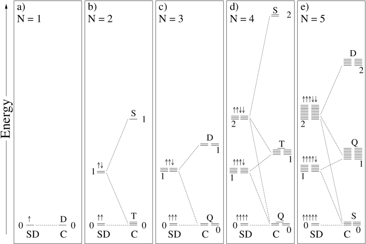
Figure 3: Energy diagram for up to five unpaired electrons. In the determination of the energy levels, equation 12 was used. The energy levels are numbered by the index j.

For the computation of multiplet energies, Noodlemans elegant and simple formula is frequently used Noodleman81 :

$$E^{LS}=(1+c)E^{BS}-cE^{HS}$$ (13)

with

$$c=\frac{1}{S_{max}+S_{min}}$$ (14)

In our notation this equation reads:

$$E^{C}_{j}=(1+c)E^{SD}_{j}-cE^{SD}_{0}$$ (15)

In contrast to equation 12, the energies are determined from $E^{SD}_{j}$ and $E^{SD}_{0}$. The Noodleman formula results in identical energy terms for up to three unpaired electrons. (Two unpaired electrons: triplet: $E_{0}^{C}=E_{0}^{SD}$, singlet: $E_{1}^{C}=2E_{1}^{SD}-E_{0}^{SD}$, three unpaired electrons: quartet: $E_{0}^{C}=E_{0}^{SD}$, doublet: $E_{1}^{C}=\frac{3}{2}E_{1}^{SD}-\frac{1}{2}E_{0}^{SD}$). For more than three unpaired electrons, as is readily verified, the Noodleman formula does not fulfill the sum rule which says that the sum of the energies of the configurations must equal the sum of the energies of the determinants they are formed from.

III General ROKS equations

Starting from

$$E_{j}^{C}=c_{j}E_{j}+c_{j-1}E_{j-1}$$ (16)

we derive single-electron ROKS equations. Using the coefficients c_j as determined by equation 12, the energy can be written in terms of energy expressions of single Slater determinants, whereby summation over half the determinants is sufficient since there are always two determinants with equal energy for which the $\alpha$ and $\beta$ spins are just interchanged.

$$\begin{split}E_{j}^{C}=&c_{j}\frac{\sum_{l=1}^{\frac{a_{j}^{SD}}{2}}E_{jl}[\rho_{jl}^{\alpha},\rho_{jl}^{\beta}]}{\frac{a_{j}^{SD}}{2}}\\ &+c_{j-1}\frac{\sum_{l=1}^{\frac{a_{j-1}^{SD}}{2}}E_{(j-1)l}[\rho_{(j-1)l}^{\alpha},\rho_{(j-1)l}^{\beta}]}{\frac{a_{j-1}^{SD}}{2}}\end{split}$$ (17)

Using the Kohn-Sham energy expression

$$\begin{split}E_{j}^{C}=&c_{j}\frac{\sum_{l=1}^{\frac{a_{j}^{SD}}{2}}\left[T[\rho_{jl}]+J[\rho_{jl}]+E_{xc}[\rho_{jl}^{\alpha},\rho_{jl}^{\beta}]+\int v(\mathbf{r})\rho_{jl}(\mathbf{r})d\mathbf{r}\right]}{\frac{a_{j}^{SD}}{2}}\\ &+c_{j-1}\frac{\sum_{l=1}^{\frac{a_{j-1}^{SD}}{2}}\left[T[\rho_{(j-1)l}]+J[\rho_{(j-1)l}]+E_{xc}[\rho_{(j-1)l}^{\alpha},\rho_{(j-1)l}^{\beta}]+\int v(\mathbf{r})\rho_{(j-1)l}(\mathbf{r})d\mathbf{r}\right]}{\frac{a_{j-1}^{SD}}{2}}\end{split}$$ (18)

the general ROKS operators for shell $i$ are obtained by functional variation:

$$\begin{split}\hat{F}_{i}=&\frac{1}{2}n_{i}\left[-\frac{1}{2}\nabla^{2}+\int\frac{\rho(\mathbf{r^{\prime}})}{|\mathbf{r}-\mathbf{r^{\prime}}|}d\mathbf{r^{\prime}}+v(\mathbf{r})\right]+\frac{1}{2}c_{j}\frac{\sum_{l=1}^{\frac{a_{j}^{SD}}{2}}\left(n_{ijl}^{\alpha}v_{xc}^{\alpha}[\rho_{jl}^{\alpha},\rho_{jl}^{\beta}]+n_{ijl}^{\beta}v_{xc}^{\beta}[\rho_{jl}^{\alpha},\rho_{jl}^{\beta}]\right)}{\frac{a_{j}^{SD}}{2}}\\ &+\frac{1}{2}c_{j-1}\frac{\sum_{l=1}^{\frac{a_{j-1}^{SD}}{2}}\left(n_{i(j-1)l}^{\alpha}v_{xc}^{\alpha}[\rho_{(j-1)l}^{\alpha},\rho_{(j-1)l}^{\beta}]+n_{i(j-1)l}^{\beta}v_{xc}^{\beta}[\rho_{(j-1)l}^{\alpha},\rho_{(j-1)l}^{\beta}]\right)}{\frac{a_{j-1}^{SD}}{2}}\end{split}$$ (19)

More details of the derivation are given for the case of two unpaired electrons in Frank98 .
For practical applications of equation 19, the n_ijl have to be determined, whereby the index $i$ denotes the - closed and open - shells, the index $j$ which numbers the energy levels is defined in equation 4, the index $l$ numbers the microstates belonging to a certain $j$. The coefficients n_ijl are given in the following section for up to five unpaired electrons.

IV Special ROKS operators

IV.1 Two unpaired electrons

The case of two unpaired electrons is described in detail in Frank98 . The energy expressions are as follows:

$$E^{C}_{0}=E^{SD}_{0}$$ (20)

$$E^{C}_{1}=2E^{SD}_{1}-E^{SD}_{0}$$ (21)

The spin densities are given in Fig. 4. The prefactors in equation 19 are listed in table 1 for the non-trivial singlet case.

Figure 4: Spin densities for the determinants that can be formed for two unpaired electrons, grouped according to their value of j. Here and in the following figures, the indices l are described with 1a, 1b, 2a, 2b etc., indicating that there are always two determinants with the same energy.

	A		B
No.	1a	1b	1a	1b
$n_{c}$	2	2	2	2
$n_{o1}^{\alpha}$	1	0	1	0
$n_{o1}^{\beta}$	0	1	0	1
$n_{o2}^{\alpha}$	1	0	0	1
$n_{o2}^{\beta}$	0	1	1	0

Table 1: Coefficients in equation 19 for two unpaired electrons.

This describes Kohn-Sham operators which explicitly read:

Triplet case:

$$\begin{split}\hat{F}_{c}=&-\frac{1}{2}\nabla^{2}+\int\frac{\rho(\mathbf{r^{\prime}})}{|\mathbf{r}-\mathbf{r^{\prime}}|}d\mathbf{r^{\prime}}+v(\mathbf{r})+\frac{1}{2}v_{xc}^{\alpha}[\rho_{A1}^{\alpha},\rho_{A1}^{\beta}]+\frac{1}{2}v_{xc}^{\beta}[\rho_{A1}^{\alpha},\rho_{A1}^{\beta}]\\ \hat{F}_{o1}=&\frac{1}{2}\left[-\frac{1}{2}\nabla^{2}+\int\frac{\rho(\mathbf{r^{\prime}})}{|\mathbf{r}-\mathbf{r^{\prime}}|}d\mathbf{r^{\prime}}+v(\mathbf{r})\right]+\frac{1}{2}v_{xc}^{\alpha}[\rho_{A1}^{\alpha},\rho_{A1}^{\beta}]\\ \hat{F}_{o2}=&\frac{1}{2}\left[-\frac{1}{2}\nabla^{2}+\int\frac{\rho(\mathbf{r^{\prime}})}{|\mathbf{r}-\mathbf{r^{\prime}}|}d\mathbf{r^{\prime}}+v(\mathbf{r})\right]+\frac{1}{2}v_{xc}^{\alpha}[\rho_{A1}^{\alpha},\rho_{A1}^{\beta}]\\ \end{split}$$ (22)

Singlet case:

$$\begin{split}\hat{F}_{c}=&-\frac{1}{2}\nabla^{2}+\int\frac{\rho(\mathbf{r^{\prime}})}{|\mathbf{r}-\mathbf{r^{\prime}}|}d\mathbf{r^{\prime}}+v(\mathbf{r})+v_{xc}^{\alpha}[\rho_{B1}^{\alpha},\rho_{B1}^{\beta}]+v_{xc}^{\beta}[\rho_{B1}^{\alpha},\rho_{B1}^{\beta}]\\ &-\frac{1}{2}(v_{xc}^{\alpha}[\rho_{A1}^{\alpha},\rho_{A1}^{\beta}]+v_{xc}^{\beta}[\rho_{A1}^{\alpha},\rho_{A1}^{\beta}])\\ \hat{F}_{o1}=&\frac{1}{2}\left[-\frac{1}{2}\nabla^{2}+\int\frac{\rho(\mathbf{r^{\prime}})}{|\mathbf{r}-\mathbf{r^{\prime}}|}d\mathbf{r^{\prime}}+v(\mathbf{r})\right]+v_{xc}^{\alpha}[\rho_{B1}^{\alpha},\rho_{B1}^{\beta}]-\frac{1}{2}v_{xc}^{\alpha}[\rho_{A1}^{\alpha},\rho_{A1}^{\beta}]\\ \hat{F}_{o2}=&\frac{1}{2}\left[-\frac{1}{2}\nabla^{2}+\int\frac{\rho(\mathbf{r^{\prime}})}{|\mathbf{r}-\mathbf{r^{\prime}}|}d\mathbf{r^{\prime}}+v(\mathbf{r})\right]+v_{xc}^{\beta}[\rho_{B1}^{\alpha},\rho_{B1}^{\beta}]-\frac{1}{2}v_{xc}^{\alpha}[\rho_{A1}^{\alpha},\rho_{A1}^{\beta}]\\ \end{split}$$ (23)

IV.2 Three unpaired electrons

$$E^{C}_{0}=E^{SD}_{0}$$ (24)

$$E^{C}_{1}=\frac{3}{2}E^{SD}_{1}-\frac{1}{2}E^{SD}_{0}$$ (25)

Figure 5: Spin densities for three unpaired electrons.

	A		B
No.	1a	1b	1a	2a	3a	1b	2b	3b
$n_{c}$	2	2	2	2	2	2	2	2
$n_{o1}^{\alpha}$	1	0	1	1	0	0	0	1
$n_{o1}^{\beta}$	0	1	0	0	1	1	1	0
$n_{o2}^{\alpha}$	1	0	1	0	1	0	1	0
$n_{o2}^{\beta}$	0	1	0	1	0	1	0	1
$n_{o3}^{\alpha}$	1	0	0	1	1	1	0	0
$n_{o3}^{\beta}$	0	1	1	0	0	0	1	1

Table 2: Coefficients in equation 19 for three unpaired electrons.

The Kohn-Sham operators for three unpaired electrons (quartet and doublet) are:

Quartet case:

$$\begin{split}\hat{F}_{c}=&-\frac{1}{2}\nabla^{2}+\int\frac{\rho(\mathbf{r^{\prime}})}{|\mathbf{r}-\mathbf{r^{\prime}}|}d\mathbf{r^{\prime}}+v(\mathbf{r})+\frac{1}{2}v_{xc}^{\alpha}[\rho_{A1}^{\alpha},\rho_{A1}^{\beta}]+\frac{1}{2}v_{xc}^{\beta}[\rho_{A1}^{\alpha},\rho_{A1}^{\beta}]\\ \hat{F}_{o1}=&\frac{1}{2}\left[-\frac{1}{2}\nabla^{2}+\int\frac{\rho(\mathbf{r^{\prime}})}{|\mathbf{r}-\mathbf{r^{\prime}}|}d\mathbf{r^{\prime}}+v(\mathbf{r})\right]+\frac{1}{2}v_{xc}^{\alpha}[\rho_{A1}^{\alpha},\rho_{A1}^{\beta}]\\ \hat{F}_{o2}=&\frac{1}{2}\left[-\frac{1}{2}\nabla^{2}+\int\frac{\rho(\mathbf{r^{\prime}})}{|\mathbf{r}-\mathbf{r^{\prime}}|}d\mathbf{r^{\prime}}+v(\mathbf{r})\right]+\frac{1}{2}v_{xc}^{\alpha}[\rho_{A1}^{\alpha},\rho_{A1}^{\beta}]\\ \hat{F}_{o3}=&\frac{1}{2}\left[-\frac{1}{2}\nabla^{2}+\int\frac{\rho(\mathbf{r^{\prime}})}{|\mathbf{r}-\mathbf{r^{\prime}}|}d\mathbf{r^{\prime}}+v(\mathbf{r})\right]+\frac{1}{2}v_{xc}^{\alpha}[\rho_{A1}^{\alpha},\rho_{A1}^{\beta}]\\ \end{split}$$ (26)

Doublet case:

$$\begin{split}\hat{F}_{c}=&-\frac{1}{2}\nabla^{2}+\int\frac{\rho(\mathbf{r^{\prime}})}{|\mathbf{r}-\mathbf{r^{\prime}}|}d\mathbf{r^{\prime}}+v(\mathbf{r})\\ &+\frac{3}{4}\Bigl{(}\frac{1}{3}(v_{xc}^{\alpha}[\rho_{B1}^{\alpha},\rho_{B1}^{\beta}]+v_{xc}^{\beta}[\rho_{B1}^{\alpha},\rho_{B1}^{\beta}]+v_{xc}^{\alpha}[\rho_{B2}^{\alpha},\rho_{B2}^{\beta}]\\ &~{}~{}~{}~{}~{}~{}~{}~{}~{}~{}+v_{xc}^{\beta}[\rho_{B2}^{\alpha},\rho_{B2}^{\beta}]+v_{xc}^{\alpha}[\rho_{B3}^{\alpha},\rho_{B3}^{\beta}]+v_{xc}^{\beta}[\rho_{B3}^{\alpha},\rho_{B3}^{\beta}])\Bigr{)}\\ &-\frac{1}{4}(v_{xc}^{\alpha}[\rho_{A1}^{\alpha},\rho_{A1}^{\beta}]+v_{xc}^{\beta}[\rho_{A1}^{\alpha},\rho_{A1}^{\beta}])\\ \hat{F}_{o1}=&\frac{1}{2}\left[-\frac{1}{2}\nabla^{2}+\int\frac{\rho(\mathbf{r^{\prime}})}{|\mathbf{r}-\mathbf{r^{\prime}}|}d\mathbf{r^{\prime}}+v(\mathbf{r})\right]\\ &+\frac{3}{4}\left(\frac{1}{3}(v_{xc}^{\alpha}[\rho_{B1}^{\alpha},\rho_{B1}^{\beta}]+v_{xc}^{\alpha}[\rho_{B2}^{\alpha},\rho_{B2}^{\beta}]+v_{xc}^{\beta}[\rho_{B3}^{\alpha},\rho_{B3}^{\beta}])\right)\\ &-\frac{1}{4}v_{xc}^{\alpha}[\rho_{A1}^{\alpha},\rho_{A1}^{\beta}]\\ \hat{F}_{o2}=&\frac{1}{2}\left[-\frac{1}{2}\nabla^{2}+\int\frac{\rho(\mathbf{r^{\prime}})}{|\mathbf{r}-\mathbf{r^{\prime}}|}d\mathbf{r^{\prime}}+v(\mathbf{r})\right]\\ &+\frac{3}{4}\left(\frac{1}{3}(v_{xc}^{\alpha}[\rho_{B1}^{\alpha},\rho_{B1}^{\beta}]+v_{xc}^{\beta}[\rho_{B2}^{\alpha},\rho_{B2}^{\beta}]+v_{xc}^{\alpha}[\rho_{B3}^{\alpha},\rho_{B3}^{\beta}])\right)\\ &-\frac{1}{4}v_{xc}^{\alpha}[\rho_{A1}^{\alpha},\rho_{A1}^{\beta}]\\ \hat{F}_{o3}=&\frac{1}{2}\left[-\frac{1}{2}\nabla^{2}+\int\frac{\rho(\mathbf{r^{\prime}})}{|\mathbf{r}-\mathbf{r^{\prime}}|}d\mathbf{r^{\prime}}+v(\mathbf{r})\right]\\ &+\frac{3}{4}\left(\frac{1}{3}(v_{xc}^{\beta}[\rho_{B1}^{\alpha},\rho_{B1}^{\beta}]+v_{xc}^{\alpha}[\rho_{B2}^{\alpha},\rho_{B2}^{\beta}]+v_{xc}^{\alpha}[\rho_{B3}^{\alpha},\rho_{B3}^{\beta}])\right)\\ &-\frac{1}{4}v_{xc}^{\alpha}[\rho_{A1}^{\alpha},\rho_{A1}^{\beta}]\\ \end{split}$$ (27)

To simplify the representation for the cases with more electrons we introduce a short notation for these equations (Tables 3 and 4).

			A
			1
	$\frac{1}{2}[~{}]$	$+\frac{1}{2}[($	$\alpha$	$\beta$	$)]$
c	2		1	1
o1	1		1	0
o2	1		1	0
o3	1		1	0

Table 3: ROKS operators for three unpaired electrons, quartet case.

			B							A
			1		2		3			1
	$\frac{1}{2}[~{}]$	$+\frac{3}{4}[\frac{1}{3}($	$\alpha$	$\beta$	$\alpha$	$\beta$	$\alpha$	$\beta$	$)]-\frac{1}{4}[($	$\alpha$	$\beta$	$)]$
c	2		1	1	1	1	1	1		1	1
o1	1		1	0	1	0	0	1		1	0
o2	1		1	0	0	1	1	0		1	0
o3	1		0	1	1	0	1	0		1	0

Table 4: ROKS operators for three unpaired electrons, doublet case.

IV.3 Four unpaired electrons

$$E^{C}_{0}=E^{SD}_{0}$$ (28)

$$E^{C}_{1}=\frac{4}{3}E^{SD}_{1}-\frac{1}{3}E^{SD}_{0}$$ (29)

$$E^{C}_{2}=3E^{SD}_{2}-2E^{SD}_{1}$$ (30)

Figure 6: Spin densities for four unpaired electrons.

Table 5 lists the coefficients for four unpaired electrons, tables 6, 7 and 8 the Fock operators in short notation.

	A		B								C
No.	1a	1b	1a	2a	3a	4a	1b	2b	3b	4b	1a	2a	3a	1b	2b	3b
$n_{c}$	2	2	2	2	2	2	2	2	2	2	2	2	2	2	2	2
$n_{o1}^{\alpha}$	1	0	1	1	1	0	0	0	0	1	1	1	1	0	0	0
$n_{o1}^{\beta}$	0	1	0	0	0	1	1	1	1	0	0	0	0	1	1	1
$n_{o2}^{\alpha}$	1	0	1	1	0	1	0	0	1	0	1	0	0	0	1	1
$n_{o2}^{\beta}$	0	1	0	0	1	0	1	1	0	1	0	1	1	1	0	0
$n_{o3}^{\alpha}$	1	0	1	0	1	1	0	1	0	0	0	0	1	1	1	0
$n_{o3}^{\beta}$	0	1	0	1	0	0	1	0	1	1	1	1	0	0	0	1
$n_{o4}^{\alpha}$	1	0	0	1	1	1	1	0	0	0	0	1	0	1	0	1
$n_{o4}^{\beta}$	0	1	1	0	0	0	0	1	1	1	1	0	1	0	1	0

Table 5: Coefficients in equation 19 for four unpaired electrons.

			A
			1
	$\frac{1}{2}[~{}]$	$+\frac{1}{2}[($	$\alpha$	$\beta$	$)]$
c	2		1	1
o1	1		1	0
o2	1		1	0
o3	1		1	0
o4	1		1	0

Table 6: ROKS operators for four unpaired electrons, quintet case.

			B									A
			1		2		3		4			1
	$\frac{1}{2}[~{}]$	$+\frac{4}{6}[\frac{1}{4}($	$\alpha$	$\beta$	$\alpha$	$\beta$	$\alpha$	$\beta$	$\alpha$	$\beta$	$)]-\frac{1}{6}[($	$\alpha$	$\beta$	$)]$
c	2		1	1	1	1	1	1	1	1		1	1
o1	1		1	0	1	0	1	0	0	1		1	0
o2	1		1	0	1	0	0	1	1	0		1	0
o3	1		1	0	0	1	1	0	1	0		1	0
o4	1		0	1	1	0	1	0	1	0		1	0

Table 7: ROKS operators for four unpaired electrons, triplet case.

			C							B
			1		2		3			1		2		3		4
	$\frac{1}{2}[~{}]$	$+\frac{3}{2}[\frac{1}{3}($	$\alpha$	$\beta$	$\alpha$	$\beta$	$\alpha$	$\beta$	$)]-[\frac{1}{4}($	$\alpha$	$\beta$	$\alpha$	$\beta$	$\alpha$	$\beta$	$\alpha$	$\beta$	$)]$
c	2		1	1	1	1	1	1		1	1	1	1	1	1	1	1
o1	1		1	0	1	0	1	0		1	0	1	0	1	0	0	1
o2	1		1	0	0	1	0	1		1	0	1	0	0	1	1	0
o3	1		0	1	0	1	1	0		1	0	0	1	1	0	1	0
o4	1		0	1	1	0	0	1		0	1	1	0	1	0	1	0

Table 8: ROKS operators for four unpaired electrons, singlet case.

IV.4 Five unpaired electrons

$$E^{C}_{0}=E^{SD}_{0}$$ (31)

$$E^{C}_{1}=\frac{5}{4}E^{SD}_{1}-\frac{1}{4}E^{SD}_{0}$$ (32)

$$E^{C}_{2}=2E^{SD}_{2}-E^{SD}_{1}$$ (33)

Figure 7: Spin densities for five unpaired electrons.

Table 9 lists the coefficients for five unpaired electrons, tables 10, 11 and 12 the Fock operators in short notation.

	A		B										C
No.	1a	1b	1a	2a	3a	4a	5a	1b	2b	3b	4b	5b	1a	2a	3a	4a	5a	6a	7a	8a	9a	10a	1b	2b	3b	4b	5b	6b	7b	8b	9b	10b
$n_{c}$	2	2	2	2	2	2	2	2	2	2	2	2	2	2	2	2	2	2	2	2	2	2	2	2	2	2	2	2	2	2	2	2
$n_{o1}^{\alpha}$	1	0	1	1	1	1	0	0	0	0	0	1	1	1	1	0	1	1	0	1	0	0	0	0	0	1	0	0	1	0	1	1
$n_{o1}^{\beta}$	0	1	0	0	0	0	1	1	1	1	1	0	0	0	0	1	0	0	1	0	1	1	1	1	1	0	1	1	0	1	0	0
$n_{o2}^{\alpha}$	1	0	1	1	1	0	1	0	0	0	1	0	1	1	0	0	1	0	1	0	1	1	0	0	1	1	0	1	0	1	0	0
$n_{o2}^{\beta}$	0	1	0	0	0	1	0	1	1	1	0	1	0	0	1	1	0	1	0	1	0	0	1	1	0	0	1	0	1	0	1	1
$n_{o3}^{\alpha}$	1	0	1	1	0	1	1	0	0	1	0	0	1	0	0	1	0	1	0	1	1	1	0	1	1	0	1	0	1	0	0	0
$n_{o3}^{\beta}$	0	1	0	0	1	0	0	1	1	0	1	1	0	1	1	0	1	0	1	0	0	0	1	0	0	1	0	1	0	1	1	1
$n_{o4}^{\alpha}$	1	0	1	0	1	1	1	0	1	0	0	0	0	0	1	1	1	0	1	1	0	1	1	1	0	0	0	1	0	0	1	0
$n_{o4}^{\beta}$	0	1	0	1	0	0	0	1	0	1	1	1	1	1	0	0	0	1	0	0	1	0	0	0	1	1	1	0	1	1	0	1
$n_{o5}^{\alpha}$	1	0	0	1	1	1	1	1	0	0	0	0	0	1	1	1	0	1	1	0	1	0	1	0	0	0	1	0	0	1	0	1
$n_{o5}^{\beta}$	0	1	1	0	0	0	0	0	1	1	1	1	1	0	0	0	1	0	0	1	0	1	0	1	1	1	0	1	1	0	1	0

Table 9: Coefficients in equation 19 for five unpaired electrons.

			A
			1
	$\frac{1}{2}[~{}]$	$+\frac{1}{2}[($	$\alpha$	$\beta$	$)]$
c	2		1	1
o1	1		1	0
o2	1		1	0
o3	1		1	0
o4	1		1	0
o5	1		1	0

Table 10: ROKS operators for five unpaired electrons, sextet case.

			B											A
			1		2		3		4		5			1
	$\frac{1}{2}[~{}]$	$+\frac{5}{8}[\frac{1}{5}($	$\alpha$	$\beta$	$\alpha$	$\beta$	$\alpha$	$\beta$	$\alpha$	$\beta$	$\alpha$	$\beta$	$)]-\frac{1}{8}[($	$\alpha$	$\beta$	$)]$
c	2		1	1	1	1	1	1	1	1	1	1		1	1
o1	1		1	0	1	0	1	0	1	0	0	1		1	0
o2	1		1	0	1	0	1	0	0	1	1	0		1	0
o3	1		1	0	1	0	0	1	1	0	1	0		1	0
o4	1		1	0	0	1	1	0	1	0	1	0		1	0
o5	1		0	1	1	0	1	0	1	0	1	0		1	0

Table 11: ROKS operators for five unpaired electrons, quartet case.

			C																					B
			1		2		3		4		5		6		7		8		9		10			1		2		3		4		5
	$\frac{1}{2}[~{}]$	$+[\frac{1}{10}($	$\alpha$	$\beta$	$\alpha$	$\beta$	$\alpha$	$\beta$	$\alpha$	$\beta$	$\alpha$	$\beta$	$\alpha$	$\beta$	$\alpha$	$\beta$	$\alpha$	$\beta$	$\alpha$	$\beta$	$\alpha$	$\beta$	$)]-\frac{1}{2}[\frac{1}{5}($	$\alpha$	$\beta$	$\alpha$	$\beta$	$\alpha$	$\beta$	$\alpha$	$\beta$	$\alpha$	$\beta$	$)]$
c	2		1	1	1	1	1	1	1	1	1	1	1	1	1	1	1	1	1	1	1	1		1	1	1	1	1	1	1	1	1	1
o1	1		1	0	1	0	1	0	0	1	1	0	1	0	0	1	1	0	0	1	0	1		1	0	1	0	1	0	1	0	0	1
o2	1		1	0	1	0	0	1	0	1	1	0	0	1	1	0	0	1	1	0	1	0		1	0	1	0	1	0	0	1	1	0
o3	1		1	0	0	1	0	1	1	0	0	1	1	0	0	1	1	0	1	0	1	0		1	0	1	0	0	1	1	0	1	0
o4	1		0	1	0	1	1	0	1	0	1	0	0	1	1	0	1	0	0	1	1	0		1	0	0	1	1	0	1	0	1	0
o5	1		0	1	1	0	1	0	1	0	0	1	1	0	1	0	0	1	1	0	0	1		0	1	1	0	1	0	1	0	1	0

Table 12: ROKS operators for five unpaired electrons, doublet case.

V Conclusions

We have derived a general explicit energy expression for restricted open-shell Kohn-Sham theory which fulfills the sum rule for the energies. If degeneracy is not prescribed and the occupation pattern is interpreted as a symmetry, the energy expression is also valid for the sum method by Ziegler, Rauk, and Baerends, and, if the exact energy expectation values are used, for ROHF itself. In the latter case the energy expression reduces to the exact energy of a single configuration Slater72 .
By inserting the Kohn-Sham expressions, we have derived ROKS operators and have given explicit expressions for these operators for up to five electrons.
The energy expression and the operators constitute just part of the restricted open-shell problem. For more than one open shell, only the high-spin solution is easily obtained. For the low-spin solutions of the ROKS equations, specific SCF algorithms turned out to be useful in the case of two open shells. In future work we want to extend these algorithms to more open shells.

VI Acknowledgment

This work was supported by the Deutsche Forschungsgemeinschaft: SFB 486 ’Manipulation von Materie auf der Nanometerskala’, SFB 749 ’Dynamik und Intermediate molekularer Transformationen’, and the Nanosystems Initiative Munich (NIM). The authors thank Sigrid Peyerimhoff and Jana Friedrichs for helpful comments and David Coughtrie for reading the manuscript.

References

• (1) C. C. J. Roothaan, Rev. Mod. Phys. 32, 179 (1960).
• (2) E. R. Davidson, Chem. Phys. Lett. 21, 565 (1973).
• (3) I. Frank, J. Hutter, D. Marx and M. Parrinello, J. Chem. Phys. 108, 4060 (1998).
• (4) S. Grimm, C. Nonnenberg and I. Frank, J. Chem. Phys. 119, 11574 (2003).
• (5) J. Friedrichs, K. Damianos and I. Frank, Chem. Phys. 347, 17 (2008).
• (6) C. Nonnenberg, S. Grimm and I. Frank, J. Chem. Phys. 119, 11585 (2003).
• (7) U. F. Röhrig, L. Guidoni, A. Laio, I. Frank and U. Röthlisberger, J. Am. Chem. Soc. 126, 15328 (2004).
• (8) C. Nonnenberg, C. Bräuchle and I. Frank, J. Chem. Phys. 122, 014311 (2005).
• (9) S. Grimm, C. Bräuchle and I. Frank, ChemPhysChem 6, 1943 (2005).
• (10) C. Nonnenberg, H. Gaub and I. Frank, ChemPhysChem 7, 1455 (2006).
• (11) I. Frank and K. Damianos, J. Chem. Phys. 126, 125105 (2007).
• (12) L. Salem, Science 191, 822 (1976).
• (13) E. R. Davidson, L. Z. Stenkamp, Int. J. Quantum Chem. Symp. 10, 21 (1976).
• (14) T. Ziegler, A. Rauk and E. Baerends, Theo. Chim. Acta 43, 261 (1977).
• (15) C. Daul, Int. J. Quant. Chem. 52, 867 (1994).
• (16) L. Noodleman, J. Chem. Phys. 74, 5737 (1981).
• (17) L. Noodleman and E.R. Davidson, Chem. Phys. 109, 131 (1986).
• (18) M. Atanasov and C. A. Daul, Chem. Phys. Lett. 379, 209 (2003).
• (19) J. C. Slater, Adv. Quantum Chem. 6, 1 (1972).