IPhT-Saclay Preprint t08/145

โ€ โ€ thanks: Supported by the Laboratoire de la Direction des Sciences de la Matiรจre du Commissariat ร  lโ€™Energie Atomique

Contact interactions in low scale string models with intersecting $D6$-branes

M. Chemtob marc.chemtob@cea.fr CEA, DSM, Institut de Physique Thรฉorique, IPhT, CNRS, MPPU, URA2306, Saclay, F-91191 Gif-sur-Yvette, FRANCE
Abstract

We evaluate the tree level four fermion string amplitudes in the TeV string mass scale models with intersecting $D6$-branes. The coefficient functions of contact interactions subsuming the contributions of string Regge resonance and winding mode excitations are obtained by subtracting out the contributions from the string massless and massive momentum modes. Numerical applications are developed for the Standard Model like solution of Cremades, Ibanez, and Marchesano for a toroidal orientifold with four intersecting $D6$-brane stacks. The chirality conserving contact interactions of the quarks and leptons are considered in applications to high energy collider and flavor changing neutral current phenomenology. The two main free parameters consist of the string and compactification mass scales, mssubscript๐‘š๐‘ m_{s} and $M_{c}$. Useful constraints on these parameters are derived from predictions for the Bhabha scattering differential cross section and for the observables associated to the mass shifts of the neutral meson systems $K-\bar{K},\ B-\bar{B},\ D-\bar{D}$ and the lepton number violating three-body leptonic decays of the charged leptons $\mu$ and $\tau$.

pacs:
12.10.Dm,11.25.Mj

I INTRODUCTION

The consideration of Dirichlet branes has led in recent years to remarkable advances in the particle physics model building. This has made possible the construction of wide classes of Standard Model realizations for type $II$ superstring theories using branes which extend along the flat spatial dimensions of $M_{4}$ and wrap around cycles of the internal space manifold. The existing two approaches employing configurations of multiple type $IIb$ branes located near orbifold singularitiesย gimpol ; gijohn ; singmod and type $IIa$ branes intersecting at anglesย berk96 , which we designate henceforth for lack of better names as setups of branes within branes and intersecting branes, respectively, are well-documented by now, thanks to the reviews inย revbib andย blumshiu05 ; blumger07 ; marche07 . The two most characteristic features of these string constructions reside in the wider freedom in choosing the string theory mass scale and in the occurrence of localized chiral fermions in the string spectrum.

Because they are amenable to experimental tests based on data from high-energy colliders and limits for rare processes, the TeV string mass scale modelsย antb90 ; lykken96 are clearly those with the greatest impact on phenomenology. In developing the string theory machinery for the physics from extra dimensions, one is especially encouraged by the applications using orbifold field theories in higher dimensional spacetimes with matter fermions which move in the bulk or are localized inside thinย add99 ; randrum99 or thickย arkan99 ; arkan00 ; mira00 ; georhailu01 domain wall branes. The theoretical and experimental aspects of collider studies of physics from extra dimensions are reviewed inย han99 ; giudice99 ; hewett02 ; cheung03 andย lands04 . The string theory framework embodies a higher degree of consistency in comparison to the field theory framework, and is also more economical thanks to a small parameter space restricted to the fundamental tension and coupling constant string parameters, ms2=1/ฮฑโ€ฒsubscriptsuperscript๐‘š2๐‘ 1superscript๐›ผโ€ฒm^{2}_{s}=1/\alpha^{\prime} and gssubscript๐‘”๐‘ g_{s}, along with adjustable parameters associated with the compactification and infrared cutoff mass scales. Several examples that qualify as TeV scale string models have been constructed within the branes within branesย kakutev98 and intersecting branesย isbtev approaches.

One important motivation for the interest in TeV scale string models is to gain insight on the hierarchy between the contributions from the various string excitations. In particular, one wishes to understand how the exchange of string Regge and winding modes compares with that of the gravitational Kaluza-Klein (KK) modes. This has a practical importance since, unlike the contributions the latter ones can be well described, in principle, within the familiar field theory framework.

The early string inspired studies were focused on models using single brane configurationsย dudas0 ; cpp00 . These have the characteristic property that the open string Regge resonance modes contribute at the tree (disk surface) level while the closed string modes contribute at the one-loop (cylinder surface) level of the string perturbation theory on the world sheet. (That the exchange of closed string modes can be viewed as a loop effect follows from the world sheet duality linking the ultraviolet and infrared regimes.) The strong constraints from the ${\cal N}=4$ supersymmetry preserved by the extremal branes of type II supergravity which saturate the BPS (Bogomolny-Prasad-Sommerfeld) bound, restrict the low-energy tree level contributions in single brane models to local operators of dimension ${\cal D}\geq 8$. Using the orbifolding mechanism, say, by placing the $D$-brane at an orbifold fixed point in order to reduce the number of preserved 4-d supercharges and produce a chiral open string spectrum, is indeed helpful towards obtaining semirealistic models but does not significantly modify the structure of string amplitudes. This is often referred as the inheritance property of orbifolds. Another characteristic of the single $D$-brane models is the insensitivity of predictions with respect to the structure of the internal space manifold. Here again the orbifold constraints on the Chan-Paton (CP) gauge factors greatly improve the description by ensuring that massless poles in channels with exotic quantum numbers cancel out. Useful applications to neutrino-nucleon elastic scattering at ultra-high energiesย cornet01 ; friess02 and to the two-body reactions at high-energy collidersย burik03 ; burik04 ; burik06 have been developed along these lines in terms of single $D$-brane models where mssubscript๐‘š๐‘ m_{s} and the CP factors are treated as free parameters. Also, building up on the initial studies of the single photon+jet signal in the high energy hadronic collider reaction, $p+p\to\gamma+j$, recent works discuss the dijet signalย ancho08 in the reaction, $p+p\to j+j$, along with signals from the various processes at the LHC modelย lust08 which could usefully test the single $D$-brane models of TeV string scale..

The multiple brane setups bring a crucial novel feature in this discussion through the presence of localized massless fermions whose contact interactions are not restricted to dimensions ${\cal D}\geq 8$. This point was first recognized by Antoniadis et al.,ย antbengier01 in the context of TeV scale string models with $Dp/D(p+4)$-branes. Finite tree level contributions were indeed found for the dimension ${\cal D}=6$ local operators coupling four fermions of which at least a single pair belongs to the non-diagonal open string sectors $(p,p+4)+(p+4,p)$. That the open string fermions localized at the intersection of $D$-branes behave in much the same way as the twisted modes of closed stringsย bersh87 ; dixon87 was realized by several authors in the context of multiple braneย hashi96 ; gava97 ; fro099 and intersecting braneย Cvetic:2003ch ; owen02 ; owen03 ; owenp03 ; KW03 ; chem06 models. The operator algebra approach for the superconformal field theory on the world sheet can be used to calculate the tree level string amplitudes. We also note as a side remark that the tools developed in recent years for the calculation of scattering amplitudes in gauge theoriesย cachazo05 and string theoriesย stietaylor07 should encourage pursuing applications for general $n$-point amplitudes at higher loop orders.

So far, the collider studies of TeV string scale models have been mostly focused on setups with single branesย dudas0 ; cpp00 and branes within branesย antbengier01 ; antorev01 ; shiusch99 , as already said above. No comparable applications exist for the intersecting branes models. Regarding the flavor physics, however, several studies have been devoted to both the branes within branesย kakutev98 and the intersecting branesย abel03 ; abeleb03 models. In parallel, a wide interest was aroused by the field theory models in flat extra dimensions with thin branesย delgado99 ; rizzo01 and thick branesย splitf03 ; masiero01 ; baren01 ; lill03 ; lill203 or in warped spacetimesย moreau06 ; csaki08 . The reader should be warned that the quoted references represent a tiny fraction of the literature on this subject.

In the present work we wish to pursue the discussion of the tree level contact interactions for four localized fermions in intersecting brane models with the view to confront the predictions against experimental data for colliders and flavor changing neutral current processes. Although the assumption of a low string mass scale is naturally paired with that of large extra space dimensions, the requirement that the string theory remains weakly coupled turns out to restrict the ratio of string to compactification scales, msโ€‹r=ms/Mcsubscript๐‘š๐‘ ๐‘Ÿsubscript๐‘š๐‘ subscript๐‘€๐‘m_{s}r=m_{s}/M_{c}, to a relatively narrow interval of $O(1)$. This circumstance has motivated us in taking the contributions from world sheet instantons into account. We evaluate the tree level string amplitudes by integrating the vacuum world sheet correlators over the moduli space of the disk surface with two pairs of massless fermion vertex operators inserted on the boundary. Since the tools for calculating open string amplitudes in intersecting brane modelsย hashi96 ; gava97 ; fro099 ; Cvetic:2003ch ; owen03 ; KW03 are well documented by now, we shall present very briefly the main formulas before proceeding to our main goal. The discussion will rely heavily on our previous workย chem06 .

We develop concrete calculations for the Standard Model solution obtained by Cremades et al.,ย CIM ; CIM2 for a toroidal orientifold with four $D6$-branes, using specifically the related family of solutions presented by Kokorelisย kokosusy02 . This is conceived as a local model (or premodel) described by a classical configuration of intersecting $D6$-branes decoupled from the gravitational interactions and the geometric moduli fields. It is encouraging that other searches of solutions for orientifolds with intersecting branes also select families of small size, as illustrated by the study focused on the $Z_{2}\times Z_{2}$ orbifold modelsย Cvetic:2004ui realizing the supersymmetric Pati-Salam model with a hidden sector, and the statistical studies of the open string landscape of vacua for the $Z_{2}\times Z_{2}$ย gmeiner05 ; douglor06 and $Z_{6-II}$ย gmeiner08 orbifolds realizing the minimal supersymmetric standard model and the Pati-Salam model with hidden sectors.

The proper identification of physics from extra dimensions presupposes that one can combine the new physics contributions with those from the Standard Model interactions in a consistent way. This condition is especially critical for the string theory applications where a satisfactory implementation of the electroweak symmetry breaking is not yet available. Rather than pursuing a full-fledged calculation, we shall adopt here a phenomenologically minded approach, similar to that used inย antbengier01 . This consists in separating out by hand in the low-energy expansion of string amplitudes the contributions from the string massless and momentum modes so as to access the contact interactions which subsume the contributions from the string Regge and winding excitations.

The exchange of massive modes from extra dimensions can also induce flavor changing interactions among fermions of different flavors which sit at points finite distances apart along the extra dimentions. These effects come on top of the flavor mixing effects generated during the electroweak gauge symmetry breaking by the trilinear Yukawa couplings of fermions to Higgs bosons. We focus here on a restricted set of hadronic and leptonic flavor observables believed to be among the most sensitive ones. To simplify calculations, we introduce certain assumptions on the flavor structure of the four fermion amplitudes which lead to an approximate factorization of the direct and indirect flavor changing effects.

The outline of the present work is as follows. Building up on our previous workย chem06 , we present in Sectionย II the tree level four fermion string amplitudes for the high energy processes of fermion-antifermion annihilation into fermion-antifermion pairs and fermion pair scattering, $f+\bar{f}\to f^{\prime}+\bar{f}^{\prime}$ and $f+f^{\prime}\to f+f^{\prime}$. We next consider an approximate construction of the contact interactions between pairs of quarks and/or leptons produced by the decoupling of string excitations. Finally, specializing to the Standard Model solution of Cremades et al.,ย CIM ; CIM2 , we present numerical results for the chirality conserving contact interactions as a function of the string and compactification mass scales and the parameters describing the separation of intersection points. The corrections to the Standard Model contributions are studied over the admissible parameter space for the string and compactification mass scales. For comprehensiveness, we provide in Appendixย A a brief review of the intersecting $D6$-brane models putting a special emphasis on the topics relating to the parameterization of the branes intersection points and the Chan-Paton gauge factors which have been lightly addressed so far. The discussion of tree level string amplitudes is complemented in Appendixย B by a review encompassing both the intersecting $D6$-brane and $D3/D7$-brane models aimed at the two-body processes of fermion-antifermion annihilation into pairs of gauge bosons and of gauge boson scattering, $f+\bar{f}\to\gamma+\gamma$ and $\gamma+\gamma\to\gamma+\gamma$.

In Sectionย III, we discuss the implications from the indirect high energy collider tests with a special focus on the Bhabha scattering differential cross section. In Sectionย IV, we examine the contributions from the flavor dependent four fermion contact interactions to the hadronic and leptonic flavor changing observables associated to the mass splitting of quark-antiquark neutral mesons and the lepton number violating three-body leptonic decays of the charged leptons. For all the above applications, we compare our predictions with experimental data in order to infer lower bounds on the string mass scale at a fixed ratio of the string to compactification mass scales.

II Tree level string amplitudes in intersecting brane models

We calculate the tree level open string amplitudes for four massless fermion modes localized at the intersection of $D6$-branes in toroidal orientifold models. After quoting in Subsec.ย II.1 the general formula for the string amplitudes and discussing its low-energy representation as infinite sums of pole terms and the subtraction prescription proposed to construct the contact interactions, we specialize in Subsec.ย II.2 to the Standard Model vacuum solution of Cremades et al.,ย CIM ; CIM2 and present in Subsec.ย II.3 numerical predictions for the contact interactions. Several notations are specified in Appendixย A which provides a brief review of intersecting $D6$-branes models. All calculations are performed with the space-time metric signature, $(-+++)$, using units where, ฮฑโ€ฒ=1/ms2=1superscript๐›ผโ€ฒ1superscriptsubscript๐‘š๐‘ 21\alpha^{\prime}={1/m_{s}^{2}}=1, except on certain occasions where $\alpha^{\prime}$ will be reinstated.

II.1 Four fermion string amplitudes and contact interactions

The open string amplitudes for four fermions localized at points of the internal manifold can be calculated most conveniently by means of the superconformal field theory on the world sheet. The basic tools were initially developed for the closed string orbifoldsย bersh87 ; dixon87 and refined in several subsequent works (seeย burwick , for instance). The application to the โ€˜twistedโ€™ or non-diagonal modes of open string sectors was discussed later for the case of branes within branesย hashi96 ; gava97 ; fro099 ; antbengier01 and of intersecting branesย Cvetic:2003ch ; owen03 ; abel03 ; chem06 .

II.1.1 String amplitudes of localized fermions

The general configuration of quantum numbers for the four fermion processes consist of two incoming conjugate fermion pairs, $f_{i}(k_{1})+\bar{f}_{j}(k_{2})+f^{\prime}_{k}(k_{3})+\bar{f}^{\prime}_{l}(k_{4})$, localized at the four intersection points, $X_{i},\ X_{j},\ X_{k},\ X_{l}\in T^{6}$, of the four $D6$-brane pairs, $(D,A),\ (A,B)$ and $(B,C),\ (C,D)$, intersecting at the angles, $\mp\theta^{I}$ and $\mp\theta^{{}^{\prime}I}$. The tree level open string amplitudes are obtained from the correlators of vertex operators inserted at points $x_{1},\ x_{2},\ x_{3},\ x_{4}$ on the disk surface boundary by integrating over the disk moduli space of the punctured disk. Using the invariance under the Mรถbius group to set, $x_{1}=0,\ x_{2}=x,\ x_{3}=1,\ x_{4}=X\to\infty$, one can write the resulting formula asย chem06

$\displaystyle{\cal A}^{\prime}_{f^{4}}\equiv{{\cal A}(V_{-\theta,(D,A),i,k_{1}}(x_{1})V_{\theta,(A,B),j,k_{2}}(x_{2})V_{-\theta^{\prime},(B,C),k,k_{3}}(x_{3})V_{\theta^{\prime},(C,D),l,k_{4}}(x_{4}))/[i(2\pi)^{4}\delta^{4}(\sum_{i}k_{i})]}$ (II.1)
=Cโ€‹(๐’ฎ1234โ€‹๐’ฏ1234โ€‹๐’ฑ1234โ€‹(s,t)+๐’ฎ1324โ€‹๐’ฏ1324โ€‹๐’ฑ1324โ€‹(u,t)+๐’ฎ1243โ€‹๐’ฏ1243โ€‹๐’ฑ1243โ€‹(s,u)),absent๐ถsubscript๐’ฎ1234subscript๐’ฏ1234subscript๐’ฑ1234๐‘ ๐‘กsubscript๐’ฎ1324subscript๐’ฏ1324subscript๐’ฑ1324๐‘ข๐‘กsubscript๐’ฎ1243subscript๐’ฏ1243subscript๐’ฑ1243๐‘ ๐‘ข\displaystyle=C\bigg{(}{\cal S}_{1234}{\cal T}_{1234}{\cal V}_{1234}(s,t)+{\cal S}_{1324}{\cal T}_{1324}{\cal V}_{1324}(u,t)+{\cal S}_{1243}{\cal T}_{1243}{\cal V}_{1243}(s,u)\bigg{)}, (II.2)

where we use the notations:

๐’ฑ1234โ€‹(s,t)=โˆซ01๐‘‘xโ€‹xโˆ’ฮฑโ€ฒโ€‹sโˆ’1โ€‹(1โˆ’x)โˆ’ฮฑโ€ฒโ€‹tโˆ’1โ€‹โˆI(2โ€‹sinโกฯ€โ€‹ฮธIIIโ€‹(x))12โ€‹โˆ‘cโ€‹lZcโ€‹lIโ€‹(x),subscript๐’ฑ1234๐‘ ๐‘กsuperscriptsubscript01differential-d๐‘ฅsuperscript๐‘ฅsuperscript๐›ผโ€ฒ๐‘ 1superscript1๐‘ฅsuperscript๐›ผโ€ฒ๐‘ก1subscriptproduct๐ผsuperscript2๐œ‹superscript๐œƒ๐ผsubscript๐ผ๐ผ๐‘ฅ12subscript๐‘๐‘™superscriptsubscript๐‘๐‘๐‘™๐ผ๐‘ฅ\displaystyle{\cal V}_{1234}(s,t)=\int_{0}^{1}dxx^{-\alpha^{\prime}s-1}(1-x)^{-\alpha^{\prime}t-1}\prod_{I}({2\sin\pi\theta^{I}\over I_{I}(x)})^{{1\over 2}}\sum_{cl}Z_{cl}^{I}(x), (II.3)
$\displaystyle{\cal T}_{1234}=T_{1234}+T_{4321},\ T_{1234}=Tr(\lambda_{1}\lambda_{2}\lambda_{3}\lambda_{4}),\ {\cal S}_{1234}=-{\cal S}_{1432}=(u_{1}^{T}\gamma^{0}\gamma_{\mu}u_{2})(u_{3}^{T}\gamma^{0}\gamma^{\mu}u_{4}),$ (II.4)
C=2โ€‹ฯ€โ€‹gsโ€‹ฮฑโ€ฒ=gฮผ2โ€‹|Lฮผ|2โ€‹ms2โ€‹Kฮผ,|Lฮผ|=โˆILฮผI,LฮผI=[(nฮผIโ€‹r1I)2+(m~ฮผIโ€‹r2I)2]12,formulae-sequence๐ถ2๐œ‹subscript๐‘”๐‘ superscript๐›ผโ€ฒsuperscriptsubscript๐‘”๐œ‡2subscript๐ฟ๐œ‡2superscriptsubscript๐‘š๐‘ 2subscript๐พ๐œ‡formulae-sequencesubscript๐ฟ๐œ‡subscriptproduct๐ผsuperscriptsubscript๐ฟ๐œ‡๐ผsuperscriptsubscript๐ฟ๐œ‡๐ผsuperscriptdelimited-[]superscriptsuperscriptsubscript๐‘›๐œ‡๐ผsuperscriptsubscript๐‘Ÿ1๐ผ2superscriptsuperscriptsubscript~๐‘š๐œ‡๐ผsuperscriptsubscript๐‘Ÿ2๐ผ212\displaystyle C=2\pi g_{s}\alpha^{\prime}={g_{\mu}^{2}|L_{\mu}|\over 2m_{s}^{2}K_{\mu}},\ |L_{\mu}|=\prod_{I}L_{\mu}^{I},\ L_{\mu}^{I}=[(n_{\mu}^{I}r_{1}^{I})^{2}+(\tilde{m}_{\mu}^{I}r_{2}^{I})^{2}]^{1\over 2}, (II.5)
s=โˆ’(k1+k2)2,t=โˆ’(k2+k3)2,u=โˆ’(k1+k3)2.formulae-sequence๐‘ superscriptsubscript๐‘˜1subscript๐‘˜22formulae-sequence๐‘กsuperscriptsubscript๐‘˜2subscript๐‘˜32๐‘ขsuperscriptsubscript๐‘˜1subscript๐‘˜32\displaystyle s=-(k_{1}+k_{2})^{2},\ t=-(k_{2}+k_{3})^{2},\ u=-(k_{1}+k_{3})^{2}. (II.6)

The string amplitude ${\cal A}^{\prime}_{f^{4}}$ in Eq.ย (II.2) is built from three reduced (partial) amplitudes associated to the cyclically inequivalent permutations of the insertion points. The second and third terms are obtained from the first term associated with the reference configuration $1234$ by substituting the mode labels $2\leftrightarrow 3$ and $3\leftrightarrow 4$, and modifying the interval of the $x$-integral from $x\in[0,1]$ to $x\in[1,\infty]$ and $x\in[-\infty,0]$. Each partial amplitude decomposes into a pair of amplitudes associated to the direct and reverse orientation permutations of the labels, corresponding to the substitutions, $2\leftrightarrow 4$ and $x\leftrightarrow(1-x)$. The requirement that the world sheet boundary is embedded in the $T^{2}_{I}$ on closed four-polygons with sides along the branes $ABCD$, can be satisfied, in general, only by a single partial amplitude, the conflict with the target space embedding forcing the other two to vanish. In our present notational conventions, only the reference term, ${\cal T}_{1234}{\cal V}_{1234}$, survives, while the other two terms, ${\cal T}_{1324}{\cal V}_{1324},\ {\cal T}_{1243}{\cal V}_{1243}$, cancel out.

The factorization of the residues of the massless pole terms from exchange of gauge bosons between fermion pairs into products of three point current vertices determines the normalization factor as, C=2โ€‹ฯ€โ€‹gsโ€‹ฮฑโ€ฒ๐ถ2๐œ‹subscript๐‘”๐‘ superscript๐›ผโ€ฒC=2\pi g_{s}\alpha^{\prime}. Using the familiar resultsย polchb for the $D$-branes of type $II$ string theories yields the formula in Eq.ย (II.2) expressing $C$ in terms of the gauge coupling constant $g_{\mu}$ of the 4-d gauge theory on the $D6_{\mu}$-brane and the volume of the three-cycle $|L_{\mu}|$ that it wraps. The same formula applies to each factor of the complete gauge group. The orientifold symmetry is taken into account by the factor $K_{\mu}$ which is assigned the value $K_{\mu}=1$ or $K_{\mu}=2$ when the brane $\mu$ is distinct or coincides with its mirror image, corresponding to the cases with $U(N)$ and extended $SO(2N)$ or $USp(2N)$ gauge symmetries, respectively. It is important to realize that the relation between the string theory gauge coupling constants, $g_{\mu}$, and their field theory counterparts which we denote momentarily by $g^{ft}_{\mu}$, also depends on the way in which the analogous field theory model is constructed. An illustrative discussion of the model dependence is presented inย KW03 . For the moment we express this relationship by the proportionality relation, $\eta g^{ft}_{\mu}=g_{\mu}$, involving the real parameter $\eta$.

The factors $I_{I}(x)$ and $Z^{I}_{cl}=\sum_{cl}e^{S^{I}_{cl}}$ for each $T_{2}^{I}$ in Eq.ย (II.2) designate the quantum (oscillator) and zero mode world sheet instanton contributions to the correlator of coordinate twist fields in the complex plane of $T^{2}_{I}$. With the choice of independent pair of cycles, ${\cal C}_{A}=(x_{1},x_{2}),\ {\cal C}_{B}=(x_{2},x_{3})$, surrounding the insertion points along the world sheet boundary, $x_{1},\cdots,x_{4}$, which map to the intersection points labeled $i,j,k,l$ in $T^{2}_{I}$, the summations in the classical partition function $Z^{I}_{cl}$ run over the large lattice generated by the one-cycles $L_{A}^{I}$ and $L_{B}^{I}$ wrapped by the $D6_{A}/D6_{B}$-branes in $T_{2}^{I}$. Going through a full circle around the cycles ${\cal C}_{A},\ {\cal C}_{B},$ induces the coordinate fields monodromies

$\displaystyle\sqrt{2}\Delta_{{\cal C}_{A}}X=2\pi(1-e^{2\pi i\theta})v_{A},\ \sqrt{2}\Delta_{{\cal C}_{B}}X=2\pi(1-e^{2\pi i\theta})v_{B},$ (II.7)

where

$\displaystyle v_{A}=p_{A}L_{A}+\delta_{ij}^{A}=(p_{A}+\epsilon_{ij}^{A})L_{A}+d_{ij}^{A},\ v_{B}=p_{B}L_{B}+\delta_{jk}^{B}=(p_{B}+\epsilon_{jk}^{B})L_{B}+d_{jk}^{B},$ (II.8)

with $p_{A},\ p_{B}\in Z$ denoting the winding numbers. The 2-d large lattices generated by the brane pairs in the complex planes of $T^{2}_{I}$ are displaced from the origin by the shifts separating the branes intersection points, $\delta^{A}=\epsilon^{A}L_{A}+d^{A},\ \delta^{B}=\epsilon^{B}L_{B}+d^{B},\ [\Re(L_{A,B}^{\star}d^{A,B})=0]$ where the real parameters $\epsilon^{A},\ \epsilon^{B}$ and $d^{A},\ d^{B}$ stand for the longitudinal and transverse components of the shift vectors relative to branes $A,\ B$. Detailed formulas for the functions $I(x)$ and $Z^{I}_{cl}$ can be found in our previous publicationย chem06 .

In the special case involving equal interbrane angles, $\theta^{I}=\theta^{{}^{\prime}I}$, which corresponds to the parallelogram $DABC$ with $D=B$ and $A=C$, the string amplitude simplifies to

$\displaystyle{\cal A}^{\prime}_{f^{4}}=C{\cal S}_{1234}\bigg{[}T_{1234}\int_{0}^{1}dxx^{-s-1}(1-x)^{-t-1}\sum_{cl}Z^{clI}_{12,34}(x)$ (II.9)
$\displaystyle+T_{4321}\int_{0}^{1}dxx^{-t-1}(1-x)^{-s-1}\sum_{cl}Z^{clI}_{43,21}(x)\bigg{]}({\sin\pi\theta^{I}\over F(x)F(1-x)})^{{1\over 2}},$ (II.10)

where

$\displaystyle Z^{clI}_{12,34}(x)=\vartheta[{{\epsilon^{A}_{12}}\atop 0}](\tau_{A})\vartheta[{{\epsilon^{B}_{23}}\atop 0}](\tau_{B})=\sum_{p_{A},\ p_{B}\in Z}e^{-{\pi}\sin\pi\theta_{I}[|(p_{A}+\epsilon^{A}_{12})L_{A}^{I}+d^{A}_{12}|^{2}{F(1-x)\over F(x)}+|(p_{B}+\epsilon^{B}_{23})L_{B}^{I}+d^{B}_{23}|^{2}{F(x)\over F(1-x)}]},$ (II.11)
$\displaystyle\tau_{A}(x)=i\sin(\pi\theta^{I})|L_{A}^{I}|^{2}{F(1-x)\over F(x)},\ \tau_{B}(x)=i\sin(\pi\theta^{I})|L_{B}^{I}|^{2}{F(x)\over F(1-x)},\ F(x)=F(\theta,1-\theta;1;x),$ (II.12)

with $F(a,b;c;x)$ denoting the Hypergeometric function and $\vartheta[{\theta\atop\phi}](\tau)$ the Jacobi Theta function. We have separated out the direct and reverse permutation terms in the quartic order trace factor, ${\cal T}_{1234}$. Verifying the equality of the factors multiplying $T_{1234}$ and $T_{4321}$ provides a useful check on calculations.

The string amplitudes for four fermions localized at the intersections of $Dp/D(p+4)$-branes are derivedย antbengier01 by a similar method to that used for intersecting branes. The resulting formulas are detailed in Appendixย B along with the similar results for the two-body processes, $f+\bar{f}\to\gamma+\gamma$ and $\gamma+\gamma\to\gamma+\gamma$.

II.1.2 Low-energy representations

The low-energy limit of compactified string theories is described by means of series expansions in powers of s/ms๐‘ subscript๐‘š๐‘ \sqrt{s}/m_{s} and (msโ€‹r)โˆ’1=Mcmssuperscriptsubscript๐‘š๐‘ ๐‘Ÿ1subscript๐‘€๐‘subscript๐‘š๐‘ (m_{s}r)^{-1}={M_{c}\over m_{s}}, where s๐‘ \sqrt{s} stands for the energy variable and $r=1/M_{c}$ for the characteristic compactification radius parameter. In the flat space limit, $r\to\infty$, both the partition function and fermion localization factors in the $x$-integral of Eq.ย (II.2) can be set to unity, $\sum_{cl}Z^{I}_{cl}=\sum_{cl}e^{-S^{I}_{cl}(x)}\to 1,\ I_{I}(x)\to 1$. Ignoring momentarily the gauge factor, one can express the string amplitude in this limit by the formula

Bโ€‹(โˆ’s,โˆ’t)โ‰กusโ€‹tโ€‹๐’ฎโ€‹(s,t)=โˆซ01๐‘‘xโ€‹xโˆ’sโˆ’1โ€‹(1โˆ’x)โˆ’tโˆ’1,๐ต๐‘ ๐‘ก๐‘ข๐‘ ๐‘ก๐’ฎ๐‘ ๐‘กsuperscriptsubscript01differential-d๐‘ฅsuperscript๐‘ฅ๐‘ 1superscript1๐‘ฅ๐‘ก1\displaystyle B(-s,-t)\equiv{u\over st}{\cal S}(s,t)=\int_{0}^{1}dxx^{-s-1}(1-x)^{-t-1}, (II.13)
[๐’ฎโ€‹(s,t)=ฮ“โ€‹(1โˆ’s)โ€‹ฮ“โ€‹(1โˆ’t)ฮ“โ€‹(1โˆ’sโˆ’t),Bโ€‹(โˆ’s,โˆ’t)โ‰กฮ“โ€‹(โˆ’s)โ€‹ฮ“โ€‹(โˆ’t)ฮ“โ€‹(โˆ’sโˆ’t)=โˆ‘n=0โˆž(โˆ’1)nโ€‹(โˆ’tโˆ’1)โ€‹โ‹ฏโ€‹(โˆ’tโˆ’n)n!โ€‹(โˆ’s+n)]delimited-[]formulae-sequence๐’ฎ๐‘ ๐‘กฮ“1๐‘ ฮ“1๐‘กฮ“1๐‘ ๐‘ก๐ต๐‘ ๐‘กฮ“๐‘ ฮ“๐‘กฮ“๐‘ ๐‘กsuperscriptsubscript๐‘›0superscript1๐‘›๐‘ก1โ‹ฏ๐‘ก๐‘›๐‘›๐‘ ๐‘›\displaystyle[{\cal S}(s,t)={\Gamma(1-s)\Gamma(1-t)\over\Gamma(1-s-t)},\ B(-s,-t)\equiv{\Gamma(-s)\Gamma(-t)\over\Gamma(-s-t)}=\sum_{n=0}^{\infty}(-1)^{n}{(-t-1)\cdots(-t-n)\over n!(-s+n)}] (II.14)

where we have exhibited in the second line the representation of Euler Beta function in terms of an infinite series of poles from s๐‘ s-channel exchange of the string Regge resonance of masses, Mn2=nโ€‹ms2,[nโˆˆZ]superscriptsubscript๐‘€๐‘›2๐‘›superscriptsubscript๐‘š๐‘ 2delimited-[]๐‘›๐‘M_{n}^{2}=nm_{s}^{2},\ [n\in Z]. At finite $r$, applying the familiar method of analytic continuation past poles to the $x$-integralย polchb with the factors $Z_{cl}$ and $I(x)$ included, produces infinite series of s๐‘ s-channel and $t$-channel pole terms at the squared masses of the open string momentum and winding modes. Since for the equal angle case associated with the brane configuration $DABC$ with $C=A,\ B=D$, the argument variable $\tau_{A}(x)\to 0$ at small $x$, one must carry beforehand the modular transformation on the Theta function with modular argument $\tau_{A}(x)$. At small $1-x$, the same applies to the Theta function with modular argument $\tau_{B}(x)$.

selecting the regions near $x=0$ in the representation of Eq.ย (II.12) yields the low-energy expansion of the string amplitude in the open string compactification modes

๐’œf4,0โ€ฒโ‰ƒCโ€‹๐’ฎ1234โ€‹(T1234|LB|โ€‹โˆ‘pA,pBโˆIฮดAโ€‹Bโˆ’MA12,B23Iโ€‹2โ€‹e2โ€‹iโ€‹ฯ€โ€‹pBโ€‹ฯต23Bโ€‹Iโˆ’s+โˆ‘IMA12,B23Iโ€‹2+T4321|LC|โ€‹โˆ‘pC,pDโˆIฮดBโ€‹Cโˆ’MB32,C43Iโ€‹2โ€‹e2โ€‹iโ€‹ฯ€โ€‹pDโ€‹ฯต32Bโ€‹Iโˆ’t+โˆ‘IMB32,C43Iโ€‹2),similar-to-or-equalssubscriptsuperscript๐’œโ€ฒsuperscript๐‘“40๐ถsubscript๐’ฎ1234subscript๐‘‡1234subscript๐ฟ๐ตsubscriptsubscript๐‘๐ดsubscript๐‘๐ตsubscriptproduct๐ผsuperscriptsubscript๐›ฟ๐ด๐ตsubscriptsuperscript๐‘€๐ผ2subscript๐ด12subscript๐ต23superscript๐‘’2๐‘–๐œ‹subscript๐‘๐ตsubscriptsuperscriptitalic-ฯต๐ต๐ผ23๐‘ subscript๐ผsubscriptsuperscript๐‘€๐ผ2subscript๐ด12subscript๐ต23subscript๐‘‡4321subscript๐ฟ๐ถsubscriptsubscript๐‘๐ถsubscript๐‘๐ทsubscriptproduct๐ผsuperscriptsubscript๐›ฟ๐ต๐ถsubscriptsuperscript๐‘€๐ผ2subscript๐ต32subscript๐ถ43superscript๐‘’2๐‘–๐œ‹subscript๐‘๐ทsubscriptsuperscriptitalic-ฯต๐ต๐ผ32๐‘กsubscript๐ผsubscriptsuperscript๐‘€๐ผ2subscript๐ต32subscript๐ถ43\displaystyle{\cal A}^{\prime}_{f^{4},0}\simeq C{\cal S}_{1234}\bigg{(}{T_{1234}\over|L_{B}|}\sum_{p_{A},p_{B}}{\prod_{I}\delta_{AB}^{-M^{I2}_{A_{12},B_{23}}}e^{2i\pi p_{B}\epsilon^{BI}_{23}}\over-s+\sum_{I}M^{I2}_{A_{12},B_{23}}}+{T_{4321}\over|L_{C}|}\sum_{p_{C},p_{D}}{\prod_{I}\delta_{BC}^{-M^{I2}_{B_{32},C_{43}}}e^{2i\pi p_{D}\epsilon^{BI}_{32}}\over-t+\sum_{I}M^{I2}_{B_{32},C_{43}}}\bigg{)}, (II.15)

where

$\displaystyle M^{I2}_{A_{ij},B_{jk}}=\sin^{2}(\pi\theta_{I})(p_{A}+\epsilon^{AI}_{ij})^{2}|L^{I}_{A}|^{2}+{p_{B}^{2}\over|L^{I}_{B}|^{2}},\ \ln\delta_{AB}=2\psi(1)-\psi(\theta^{I})-\psi(1-\theta^{I}),$ (II.16)

and $\psi(z)$ is the PolyGamma function. The squared masses, $M^{2}_{A,B}$, consist of string momentum modes of the sector $(B,B)$ along the compact directions wrapped by the brane $B$, and string winding modes of the sector $(A,A)$ for strings stretched transversally to the cycle $L_{B}$. Expressing the normalization factor C=2โ€‹ฯ€โ€‹gs๐ถ2๐œ‹subscript๐‘”๐‘ C=2\pi g_{s} in the s๐‘ s- and $t$-channel pole terms in terms of the corresponding parameters of branes $B$ and $C$, respectively, then comparison with the amplitude of the analogous field theory leads to the identifications, ${g_{B}^{2}\over 2K_{B}}T_{1234}=(g_{B}^{ft})^{2}\sum_{a}(T^{a})_{12}(T^{a})_{34}$ and ${g_{C}^{2}\over 2K_{C}}=(g_{C}^{ft})^{2}\sum_{a}(T^{a})_{23}(T^{a})_{14}$, where $a$ labels the Lie algebra generators of the gauge groups on branes $B,\ C$. The extra factor $2$ in the denominator accounts for the field theory normalization convention used for the field theory gauge coupling constant, corresponding to the gauge current vertex, $<J^{a}_{\lambda}(0)>=g_{A}T^{a}\gamma_{\lambda},\ [Trace(T_{a}T_{b})={1\over 2}\delta_{ab}]$.

The residues $\delta_{AB}^{-M_{A,B}^{2}}$ of the poles at s=MA,B2๐‘ subscriptsuperscript๐‘€2๐ด๐ตs=M^{2}_{A,B} (and the similar residues of the poles at $t=M^{2}_{B,C}$) represent the squares of the form factors for the three point couplings of fermion pairs localized at the $D6_{A}/D6_{B}$ brane intersections with the open string states of mass $M_{A,B}$ from the sectors $(A,A)$ and $(B,B)$. As the interbrane angle runs over the defining interval, $\theta^{I}\in[0,1]$ in the $T^{2}_{I}$ tori, $\ln\delta^{I}_{AB}$ asymptotes to $\cot(\pi\theta^{I})\to+\infty$ at the interval end points while reaching the minimum value, $\ln\delta^{I}_{AB}\simeq 2.77$, at the mid-point $\theta^{I}={1\over 2}$. The divergence of $\ln\delta^{I}_{AB}$ at $\theta^{I}=0$ and $1$ implies then the absence of contributions from the exchange of string compactification modes for parallel branes, as expected by virtue of the momentum conservation. The form factor, ${\cal F}_{AB}(p_{B})=\delta_{AB}^{-M_{A,B}^{2}/2}$, representing the cost for a fermion particle to absorb the gauge boson momentum $p_{B}$, arises as a consequence of the $D$-brane fuzziness caused by the finite spatial extension of string modes. Its configuration space representation, ${\cal F}_{AB}(y)$, can be evaluated by writing the three point coupling of fermion pairs to the momentum modes of the $D6_{B}$-brane gauge connection field, $A^{B}_{\mu}(x,y)$, as a Fourier integral over the cycle of radius $L_{B}$

$\displaystyle\int_{0}^{\pi|L_{B}|}dyA^{B}_{\mu}(x,y){\cal F}_{AB}(y-y_{i}^{B})\equiv\sqrt{2\over\pi|L_{B}|}\sum_{p_{B}}N_{p_{B}}[A^{B(p_{B})}_{\mu}(x)\int_{0}^{\pi|L_{B}|}dy\cos({yp_{B}\over|L_{B}|}){\cal F}_{AB}(y-y_{i}^{B})+\cdots]$ (II.17)
$\displaystyle=\sqrt{2\over\pi|L_{B}|}\sum_{p_{B}}N_{p_{B}}[A^{B(p_{B})}_{\mu}(x)\delta_{AB}^{-{p_{B}^{2}/(2|L_{B}|^{2})}}e^{ip_{B}y_{i}^{B}\over|L_{B}|}+\cdots],$ (II.18)

with the resulting formula

$\displaystyle{\cal F}_{AB}(y)\simeq\sqrt{2\over\pi\ln\delta_{AB}}e^{-{y^{2}\over 2|L_{B}|^{2}\ln\delta_{AB}}},\ [y_{i}^{B}=2\pi\epsilon_{i}^{B}|L_{B}|]$ (II.19)

where $y$ parameterizes the points on the $L_{B}$ cycle which has been described here by the orbifold $S^{1}/Z_{2}$ of length $\pi|L_{B}|$; $y_{i}^{B}$ denotes the position of the fermion mode; $N_{p_{B}}=1$ for pBโ‰ 0subscript๐‘๐ต0p_{B}\neq 0 and $N_{p_{B}}=1/\sqrt{2}$ for $p_{B}=0$; and the central dots stand for the sine stationary modes. The above approximate formula for ${\cal F}_{AB}(y)$ becomes exact in the large radius limit, $|L_{B}|\to\infty$. The exchange of massive KK gauge bosons contributes to the four fermion amplitude a sum of pole terms with residue factors, $e^{2\pi ip_{B}\epsilon^{B}_{jk}}\delta_{AB}^{-p_{B}^{2}/|L_{B}|^{2}}$, where $\epsilon^{B}_{jk}$ denotes the relative distance along the brane $B$, as expected by comparison with Eq.ย (II.16). A similar analysis holds for the momentum modes associated with the brane $C$. By contrast, there is no field theory interpretation for the form factors accompanying the coupling of localized fermions to the open string winding modes.

To illustrate further how the form factor originates within the field theory framework, we consider the toy-like 5-d $U(1)$ gauge theory with the fifth dimension compactified along the orbifold segment, $y\in[0,\pi|L_{B}|]$, assuming that the chiral fermions are trapped near the boundaries by some soliton kink solution involving a scalar field coupled to the fermions. Making use of the Gaussian ansatz for the normalizable zero mode wave function of a fermion localized at $y_{i}^{B}$,

$\displaystyle\psi^{(0)}_{i}(y)=Ne^{-(y-y_{i}^{B})^{2}/(2\sigma^{2}\pi^{2})},\ [\int_{0}^{\pi|L_{B}|}dy\psi^{(0)\star}_{i}(y)\psi^{(0)}_{i}(y)=1,\ N\simeq({2\over\pi^{3\over 2}\sigma})^{1\over 2}]$ (II.20)

where the normalization integral determining $N$ has been evaluated in the limit $L_{B}\to\infty$, we infer the gauge vertex coupling

$\displaystyle\sum_{p_{B}}N_{p_{B}}A_{\mu}^{B(p_{B})}(x)\int_{0}^{\pi|L_{B}|}dy\psi^{(0)\star}_{i}(y)\psi^{(0)}_{i}(y)\cos({yp_{B}\over|L_{B}|})\simeq\sum_{p_{B}}N_{p_{B}}e^{-{\pi^{2}\sigma^{2}p_{B}^{2}\over 4|L_{B}|^{2}}}\cos({y_{i}^{B}p_{B}\over|L_{B}|}).$ (II.21)

Comparison with the form factor ${\cal F}_{AB}(p_{B})$ in Eq.ย (II.19) allows us to identify the half-width parameter as, $\sigma\simeq\sqrt{2\ln\delta_{AB}}/\pi$. The above result for the form factor of fermion modes localized at intersecting branes agrees with that derivedย antbengier01 for the fermion modes of the non-diagonal sectors of $D3/D7$-branes, where $\theta^{I}={1\over 2}$. (The half-width parameter inย antbengier01 , which we distinguish here by the suffix label ${ABL}$, is related to ours as, $\sigma_{ABL}=\sigma\pi/\sqrt{2}$. For later reference, we note that our half-width parameter $\sigma$ identifies with the parameter denoted $\sigma$ inย lill03 .) It is of interest to note that a similar form factor also arises in the string amplitude for emission of a massive graviton mode $G(M_{cl})$ in the two-body reaction, $f+\bar{f}\to\gamma+G(M_{cl})$, with the characteristic dependence on the mass $M_{cl}$ of the closed string modeย cpp00 , โ„ฑGโ€‹(Mcโ€‹l)=eโˆ’lnโก(2)โ€‹Mcโ€‹l2/ms2subscriptโ„ฑ๐บsubscript๐‘€๐‘๐‘™superscript๐‘’2superscriptsubscript๐‘€๐‘๐‘™2superscriptsubscript๐‘š๐‘ 2{\cal F}_{G}(M_{cl})=e^{-\ln(2)M_{cl}^{2}/m_{s}^{2}}. Both the present string form factor and the one derived above, โ„ฑoโ€‹pโ€‹(Moโ€‹p)=eโˆ’Moโ€‹p2โ€‹lnโก(ฮด)/(2โ€‹ms2)subscriptโ„ฑ๐‘œ๐‘subscript๐‘€๐‘œ๐‘superscript๐‘’subscriptsuperscript๐‘€2๐‘œ๐‘๐›ฟ2superscriptsubscript๐‘š๐‘ 2{\cal F}_{op}(M_{op})=e^{-M^{2}_{op}\ln(\delta)/(2m_{s}^{2})}, should be distinguished from the form factor arising from the quantum fluctuations of branesย bando99 ; hisano99 ; murawells01 . Using a quantum field theory treatment of the Nambu-Goto action for domain walls with the transverse coordinate $y$ promoted to the would-be light Nambu-Goldstone scalar field associated to the spontaneous breaking of translational invariance, Bando et al.,ย bando99 found that the coupling to momentum modes in the effective 4-d action is accompanied by the recoil form factor

$\displaystyle{\cal F}_{rec}(M)\simeq e^{-\Delta^{2}M^{2}},\ [\Delta^{2}={M_{F}^{2}\over(4\pi)^{2}\tau_{p}}={M_{F}^{2}g^{2}_{Dp}\over 4m_{s}^{4}},\ M^{2}={p^{2}\over|L_{B}|^{2}}]$ (II.22)

where $M_{F}$ denotes the ultraviolet mass cut-off for the field theory on the domain wall whose tension parameter has been identified above to that of the $Dp$-brane, ฯ„Dโ€‹p=[ms2/(2โ€‹ฯ€โ€‹gDโ€‹p)]2subscript๐œ๐ท๐‘superscriptdelimited-[]superscriptsubscript๐‘š๐‘ 22๐œ‹subscript๐‘”๐ท๐‘2\tau_{Dp}=[m_{s}^{2}/(2\pi g_{Dp})]^{2}, with gauge coupling constant $g_{Dp}$. The specific case of a soliton domain wall is discussed in ย hisano99 . From the comparison of the ratio of half-width parameters for the form factors associated to the brane fuzziness and recoil, ฮ”2:ฯƒ2=MF2โ€‹gDโ€‹p24โ€‹ms4:lnโกฮด2โ€‹ms2โ‰ƒgDโ€‹p22โ€‹lnโกฮด:1:superscriptฮ”2superscript๐œŽ2superscriptsubscript๐‘€๐น2subscriptsuperscript๐‘”2๐ท๐‘4superscriptsubscript๐‘š๐‘ 4:similar-to-or-equals๐›ฟ2superscriptsubscript๐‘š๐‘ 2subscriptsuperscript๐‘”2๐ท๐‘2๐›ฟ:1\Delta^{2}:\sigma^{2}={M_{F}^{2}g^{2}_{Dp}\over 4m_{s}^{4}}:{\ln\delta\over 2m_{s}^{2}}\simeq{g^{2}_{Dp}\over 2\ln\delta}:1, where we have assumed in the second stage, MFโ‰ƒmssimilar-to-or-equalssubscript๐‘€๐นsubscript๐‘š๐‘ M_{F}\simeq m_{s}, we conclude that the suppression effect from brane recoil is parametrically weaker than that from the string finite size. This property was previously discussed inย cpp00 .

II.1.3 Contact interactions and flavor structure

The four fermion string amplitude receives infrared divergent contributions from the $x$-integral boundaries which correspond to the massless s,t๐‘ ๐‘กs,\ t channel pole terms from gauge bosons exchange. One way to regularize these harmless poles is to subtract out the small regions in the $x$-integral near the end points $x=0,\ x=1$, while adding up the corresponding pole terms by hand, as described by the subtraction, ๐’œโ†’๐’œโˆ’(โˆ’๐’œspโ€‹oโ€‹lโ€‹e+๐’œ|x=0)โˆ’(โˆ’๐’œtpโ€‹oโ€‹lโ€‹e+๐’œ|x=1)โ†’๐’œ๐’œsuperscriptsubscript๐’œ๐‘ ๐‘๐‘œ๐‘™๐‘’evaluated-at๐’œ๐‘ฅ0superscriptsubscript๐’œ๐‘ก๐‘๐‘œ๐‘™๐‘’evaluated-at๐’œ๐‘ฅ1{\cal A}\to{\cal A}-(-{\cal A}_{s}^{pole}+{\cal A}|_{x=0})-(-{\cal A}_{t}^{pole}+{\cal A}|_{x=1}). To account for the electroweak symmetry breaking, one can use the same prescription where the added pole terms correspond to the contributions from exchange of the physical gauge bosons with the observed finite values of the masses. For the four fermion coupling $(\bar{f}_{H}\gamma_{\mu}f_{H})(\bar{f}^{\prime}_{H^{\prime}}\gamma^{\mu}f^{\prime}_{H^{\prime}})$ in the electrically charge neutral channel for the $\gamma,\ Z$ gauge bosons, this is illustrated by the substitution, 1sโ†’1s+aHโ€‹(f)โ€‹aHโ€ฒโ€‹(fโ€ฒ)sโˆ’mZ2โ†’1๐‘ 1๐‘ subscript๐‘Ž๐ป๐‘“subscript๐‘Žsuperscript๐ปโ€ฒsuperscript๐‘“โ€ฒ๐‘ superscriptsubscript๐‘š๐‘2{1\over s}\to{1\over s}+{a_{H}(f)a_{H^{\prime}}(f^{\prime})\over s-m_{Z}^{2}}, where $a_{H}(f)$ denote the $Z$ boson vertex couplings. A similar replacement holds for the $t-$channel poles.

The contact interactions, subsuming the contributions from the massive string Regge and winding excitations, can be constructed in a similar way by subtracting also the pole terms associated to the string momentum excitations, as illustrated by the schematic formula

๐’œcโ€‹oโ€‹nโ€‹tโ€‹aโ€‹cโ€‹tโ€ฒ=๐’œโ€ฒโˆ’๐’œs,Kโ€‹Kโ€ฒโˆ’๐’œt,Kโ€‹Kโ€ฒ.subscriptsuperscript๐’œโ€ฒ๐‘๐‘œ๐‘›๐‘ก๐‘Ž๐‘๐‘กsuperscript๐’œโ€ฒsubscriptsuperscript๐’œโ€ฒ๐‘ ๐พ๐พsubscriptsuperscript๐’œโ€ฒ๐‘ก๐พ๐พ\displaystyle{\cal A}^{\prime}_{contact}={\cal A}^{\prime}-{\cal A}^{\prime}_{s,KK}-{\cal A}^{\prime}_{t,KK}. (II.23)

The same subtraction procedure was previously used to defineย antbengier01 the contact interactions in models with $Dp/D(p+4)$-branes. For consistency, we remove the sโˆ’limit-from๐‘ s-channel terms only for the configurations of intersection points with $i=j$ or $\epsilon^{A}_{ij}=0,$ and the $t-$channel terms only for those with $k=l$ or $\epsilon^{B}_{jk}=0$. No subtraction of momentum modes is needed in the cases, iโ‰ jโ‰ k๐‘–๐‘—๐‘˜i\neq j\neq k or ฯตiโ€‹jAโ‰ 0,ฯตjโ€‹kBโ‰ 0formulae-sequencesubscriptsuperscriptitalic-ฯต๐ด๐‘–๐‘—0subscriptsuperscriptitalic-ฯต๐ต๐‘—๐‘˜0\epsilon^{A}_{ij}\neq 0,\ \epsilon^{B}_{jk}\neq 0, where the thresholds for the momentum modes are separated by a finite gap corresponding to the mass terms, $\epsilon_{A}^{2}|L_{A}|^{2}$. One motivation for excluding the KK towers from the contact interactions is simply that it is always possible to include separately their contributions through the familiar field theory treatment, suitably generalized by the inclusion of form factors. In the flat space limit, $L_{B}\to\infty$, with the brane form factors set to unity, $\delta^{-M_{A,B}^{2}}\to 1$, the contact interactions from KK modes are described by the approximate formula

LEโ€‹Fโ€‹F=gB22โ€‹ms2โ€‹๐’ฎ1234โ€‹๐’ฏ1234โ€‹โˆ‘pโˆˆZฮดโˆ’p2/|LB|2(p2/|LB|2โˆ’s)โ‰ƒgB22โ€‹ms2โ€‹Snโ€‹(msโ€‹|LB|)n(nโˆ’2)โ€‹๐’ฎ1234โ€‹๐’ฏ1234,subscript๐ฟ๐ธ๐น๐นsuperscriptsubscript๐‘”๐ต22superscriptsubscript๐‘š๐‘ 2subscript๐’ฎ1234subscript๐’ฏ1234subscript๐‘๐‘superscript๐›ฟsuperscript๐‘2superscriptsubscript๐ฟ๐ต2superscript๐‘2superscriptsubscript๐ฟ๐ต2๐‘ similar-to-or-equalssuperscriptsubscript๐‘”๐ต22superscriptsubscript๐‘š๐‘ 2subscript๐‘†๐‘›superscriptsubscript๐‘š๐‘ subscript๐ฟ๐ต๐‘›๐‘›2subscript๐’ฎ1234subscript๐’ฏ1234\displaystyle L_{EFF}={g_{B}^{2}\over 2m_{s}^{2}}{\cal S}_{1234}{\cal T}_{1234}\sum_{p\in Z}{\delta^{-p^{2}/|L_{B}|^{2}}\over(p^{2}/|L_{B}|^{2}-s)}\simeq{g_{B}^{2}\over 2m_{s}^{2}}{S_{n}(m_{s}|L_{B}|)^{n}\over(n-2)}{\cal S}_{1234}{\cal T}_{1234}, (II.24)

where $S_{n}={2\pi^{n/2}\over\Gamma(n/2)}$ with $n=D-4$ denoting the number of real dimensions of the wrapped cycle.

In the kinematic regime where mass parameters and energies are negligible in comparison to mssubscript๐‘š๐‘ m_{s}, the four fermion local couplings are dominated by the chirality conserving couplings of dimension ${\cal D}=6$. The corresponding terms in the Standard Model effective Lagrangian are represented in the left and right chirality basis of fermion field operators by the general structure

$\displaystyle L_{EFF}=\sum_{f,f^{\prime}}[G_{ff^{\prime}}^{LL}(\bar{f}_{L}\gamma_{\mu}f_{L})(\bar{f}^{\prime}_{L}\gamma^{\mu}f^{\prime}_{L})+G_{ff^{\prime}}^{LR}(\bar{f}_{L}\gamma_{\mu}f_{L})(\bar{f}^{\prime}_{R}\gamma^{\mu}f^{\prime}_{R})$ (II.25)
$\displaystyle+G_{ff^{\prime}}^{RL}(\bar{f}_{R}\gamma_{\mu}f_{R})(\bar{f}^{\prime}_{L}\gamma^{\mu}f^{\prime}_{L})+G_{ff^{\prime}}^{RR}(\bar{f}_{R}\gamma_{\mu}f_{R})(\bar{f}^{\prime}_{R}\gamma^{\mu}f^{\prime}_{R})],$ (II.26)

where $G_{ff^{\prime}}^{HH^{\prime}}=\eta_{HH^{\prime}}{4\pi\over 2\Lambda^{ff^{\prime}2}_{HH^{\prime}}}$, with $H,\ H^{\prime}=(L,R)$. We follow the notational conventions for the coefficients $G_{ff^{\prime}}^{HH^{\prime}}$ commonly adopted in the context of composite modelsย peskin83 , with $\eta_{HH^{\prime}}$ denoting relative $\pm$ signs and $\Lambda^{ff^{\prime}2}_{HH^{\prime}}$ the characteristic squared mass scale parameters. For later reference, we also quote the effective Lagrangian of use in leptonic collider applications

$\displaystyle L_{EFF}=\sum_{f,H,H^{\prime}}{4\pi\eta_{HH^{\prime}}\over\Lambda^{ef2}_{HH^{\prime}}(1+\delta_{ef})}G_{ef}^{HH^{\prime}}(\bar{e}_{H}\gamma_{\mu}e_{H})(\bar{f}_{H^{\prime}}\gamma^{\mu}f_{H^{\prime}}),$ (II.27)

where $\delta_{ef}=1$ if $e=f$ and $\delta=0$ if eโ‰ f๐‘’๐‘“e\neq f. The left chirality basis for the fermion fields is related to the mixed left-right chirality basis by, LโˆผRcโฃโ€ similar-to๐ฟsuperscript๐‘…๐‘โ€ L\sim R^{c\dagger}, thus implying the identity, $(\bar{L}_{1}\gamma^{\mu}L_{2})=(\bar{R}_{2}^{c}\gamma^{\mu}R_{1}^{c})$, and the Fierz-Michel identities for the quartic order matrix elements,

$\displaystyle(\bar{L}_{1}\gamma^{\mu}L_{2})(\bar{R}_{3}\gamma_{\mu}R_{4})=2(\bar{L}_{1}R_{4})(\bar{R}_{3}L_{2}),\ (\bar{L}_{1}\gamma^{\mu}L_{2})(\bar{L}_{3}\gamma_{\mu}L_{4})=-(\bar{L}_{1}\gamma^{\mu}L_{4})(\bar{L}_{3}\gamma_{\mu}L_{2}),$ (II.28)

where $L,\ R$ denote c-number (commuting) Dirac spinors. The comparison with Eq.ย (II.2) yields the explicit formula for the dimensionless coefficient functions $g_{ff^{\prime}}^{HH^{\prime}}(L_{\mu})$ defined by

gfโ€‹fโ€ฒHโ€‹Hโ€ฒโ‰กms2โ€‹Kฮผ2โ€‹ฯ€โ€‹gฮผ2โ€‹Gfโ€‹fโ€ฒHโ€‹Hโ€ฒ=ฮทHโ€‹Hโ€ฒโ€‹ms2โ€‹Kฮผฮ›Hโ€‹Hโ€ฒfโ€‹fโ€ฒโ€‹2โ€‹gฮผ2=|Lฮผ|4โ€‹ฯ€โ€‹โˆซ01๐‘‘xโ€‹xโˆ’sโˆ’1โ€‹(1โˆ’x)โˆ’tโˆ’1โ€‹โˆI(2โ€‹sinโกฯ€โ€‹ฮธIIIโ€‹(x))12โ€‹โˆ‘cโ€‹lZcโ€‹lI,superscriptsubscript๐‘”๐‘“superscript๐‘“โ€ฒ๐ปsuperscript๐ปโ€ฒsuperscriptsubscript๐‘š๐‘ 2subscript๐พ๐œ‡2๐œ‹superscriptsubscript๐‘”๐œ‡2superscriptsubscript๐บ๐‘“superscript๐‘“โ€ฒ๐ปsuperscript๐ปโ€ฒsubscript๐œ‚๐ปsuperscript๐ปโ€ฒsuperscriptsubscript๐‘š๐‘ 2subscript๐พ๐œ‡subscriptsuperscriptฮ›๐‘“superscript๐‘“โ€ฒ2๐ปsuperscript๐ปโ€ฒsuperscriptsubscript๐‘”๐œ‡2subscript๐ฟ๐œ‡4๐œ‹superscriptsubscript01differential-d๐‘ฅsuperscript๐‘ฅ๐‘ 1superscript1๐‘ฅ๐‘ก1subscriptproduct๐ผsuperscript2๐œ‹superscript๐œƒ๐ผsubscript๐ผ๐ผ๐‘ฅ12subscript๐‘๐‘™subscriptsuperscript๐‘๐ผ๐‘๐‘™\displaystyle g_{ff^{\prime}}^{HH^{\prime}}\equiv{m_{s}^{2}K_{\mu}\over 2\pi g_{\mu}^{2}}G_{ff^{\prime}}^{HH^{\prime}}=\eta_{HH^{\prime}}{m_{s}^{2}K_{\mu}\over\Lambda^{ff^{\prime}2}_{HH^{\prime}}g_{\mu}^{2}}={|L_{\mu}|\over 4\pi}\int_{0}^{1}dxx^{-s-1}(1-x)^{-t-1}\prod_{I}({2\sin\pi\theta^{I}\over I_{I}(x)})^{{1\over 2}}\sum_{cl}Z^{I}_{cl}, (II.29)

such that the string four fermion amplitude reads as, ๐’œf4=2โ€‹ฯ€โ€‹gฮผ2ms2โ€‹Kฮผโ€‹gfโ€‹fโ€ฒHโ€‹Hโ€ฒโ€‹<๐’ฎ1234>Hโ€‹Hโ€ฒโ€‹<๐’ฏ1234>fโ€‹fโ€ฒ.subscript๐’œsuperscript๐‘“42๐œ‹subscriptsuperscript๐‘”2๐œ‡superscriptsubscript๐‘š๐‘ 2subscript๐พ๐œ‡superscriptsubscript๐‘”๐‘“superscript๐‘“โ€ฒ๐ปsuperscript๐ปโ€ฒsubscriptexpectationsubscript๐’ฎ1234๐ปsuperscript๐ปโ€ฒsubscriptexpectationsubscript๐’ฏ1234๐‘“superscript๐‘“โ€ฒ{\cal A}_{f^{4}}={2\pi g^{2}_{\mu}\over m_{s}^{2}K_{\mu}}g_{ff^{\prime}}^{HH^{\prime}}<{\cal S}_{1234}>_{HH^{\prime}}<{\cal T}_{1234}>_{ff^{\prime}}. For convenience, we shall employ in the sequel a similar notational convention for the string amplitudes for fermions of fixed chiralities.

To make contact with the amplitudes of physical processes involving the mass eigenstate fields, we need to perform the familiar bi-unitary linear transformations linking the above gauge basis to the mass eigenvector basis, fโ†’VLfโฃโ€ โ€‹f,fcโ†’VRfโ€‹Tโ€‹fc,[f=q,l]formulae-sequenceโ†’๐‘“superscriptsubscript๐‘‰๐ฟ๐‘“โ€ ๐‘“โ†’superscript๐‘“๐‘superscriptsubscript๐‘‰๐‘…๐‘“๐‘‡superscript๐‘“๐‘delimited-[]๐‘“๐‘ž๐‘™f\to V_{L}^{f\dagger}f,\ f^{c}\to V_{R}^{fT}f^{c},\ [f=q,l] which read in the left-right chirality basis as, fHโ†’VHfโฃโ€ โ€‹fH,[H=L,R]โ†’subscript๐‘“๐ปsuperscriptsubscript๐‘‰๐ป๐‘“โ€ subscript๐‘“๐ปdelimited-[]๐ป๐ฟ๐‘…f_{H}\to V_{H}^{f\dagger}f_{H},\ [H=L,R]. The flavor mixing matrices, $V^{f}_{L},\ V^{f}_{R}$, are determined through the diagonalization of the fermion mass matrices in generation space, VRfโ€‹Mfโ€‹VLfโฃโ€ =(Mf)dโ€‹iโ€‹aโ€‹gsuperscriptsubscript๐‘‰๐‘…๐‘“subscript๐‘€๐‘“superscriptsubscript๐‘‰๐ฟ๐‘“โ€ subscriptsubscript๐‘€๐‘“๐‘‘๐‘–๐‘Ž๐‘”V_{R}^{f}M_{f}V_{L}^{f\dagger}=(M_{f})_{diag}, but in a partial way since the Standard Model contributions from the quarks and leptons only depend on the products, VCโ€‹Kโ€‹M=VLuโ€‹VLdโฃโ€ subscript๐‘‰๐ถ๐พ๐‘€superscriptsubscript๐‘‰๐ฟ๐‘ขsuperscriptsubscript๐‘‰๐ฟ๐‘‘โ€ V_{CKM}=V_{L}^{u}V_{L}^{d\dagger} and Vโ€ฒ=VLฮฝโ€‹VLeโฃโ€ superscript๐‘‰โ€ฒsuperscriptsubscript๐‘‰๐ฟ๐œˆsuperscriptsubscript๐‘‰๐ฟ๐‘’โ€ V^{\prime}=V_{L}^{\nu}V_{L}^{e\dagger}, where the suffix label CKM refers to the quarks Cabibbo-Kobayashi-Maskawa matrix. The effective Lagrangian of dimension ${\cal D}=6$ in the vector spaces of the fermions generation and mass basis fields can now be expressed as

$\displaystyle L_{EFF}=\sum_{f,f^{\prime}}\sum_{H,H^{\prime}}G^{HH^{\prime}}_{ij,kl}[(\bar{f}_{iH}\gamma^{\mu}f_{jH})(\bar{f}^{\prime}_{kH^{\prime}}\gamma_{\mu}f^{\prime}_{lH^{\prime}})]_{flav}+H.c.$ (II.30)
=โˆ‘f,fโ€ฒโˆ‘H,Hโ€ฒG~iโ€‹j,kโ€‹lHโ€‹Hโ€ฒโ€‹[(fยฏiโ€‹Hโ€‹ฮณฮผโ€‹fjโ€‹H)โ€‹(fยฏkโ€‹Hโ€ฒโ€ฒโ€‹ฮณฮผโ€‹flโ€‹Hโ€ฒโ€ฒ)]mโ€‹aโ€‹sโ€‹s+H.c.,formulae-sequenceabsentsubscript๐‘“superscript๐‘“โ€ฒsubscript๐ปsuperscript๐ปโ€ฒsubscriptsuperscript~๐บ๐ปsuperscript๐ปโ€ฒ๐‘–๐‘—๐‘˜๐‘™subscriptdelimited-[]subscriptยฏ๐‘“๐‘–๐ปsuperscript๐›พ๐œ‡subscript๐‘“๐‘—๐ปsubscriptsuperscriptยฏ๐‘“โ€ฒ๐‘˜superscript๐ปโ€ฒsubscript๐›พ๐œ‡subscriptsuperscript๐‘“โ€ฒ๐‘™superscript๐ปโ€ฒ๐‘š๐‘Ž๐‘ ๐‘ ๐ป๐‘\displaystyle=\sum_{f,f^{\prime}}\sum_{H,H^{\prime}}\tilde{G}^{HH^{\prime}}_{ij,kl}[(\bar{f}_{iH}\gamma^{\mu}f_{jH})(\bar{f}^{\prime}_{kH^{\prime}}\gamma_{\mu}f^{\prime}_{lH^{\prime}})]_{mass}+H.c., (II.31)

where

G~iโ€‹j,kโ€‹lHโ€‹Hโ€ฒโ‰ก2โ€‹ฯ€โ€‹gA2ms2โ€‹KAโ€‹g~iโ€‹j,kโ€‹lHโ€‹Hโ€ฒ=Giโ€ฒโ€‹jโ€ฒ,kโ€ฒโ€‹lโ€ฒHโ€‹Hโ€ฒโ€‹(VHโ€‹iโ€‹iโ€ฒfโ€‹VHโ€‹jโ€‹jโ€ฒfโฃโ‹†)โ€‹(VHโ€ฒโ€‹kโ€‹kโ€ฒfโ€ฒโ€‹VHโ€ฒโ€‹lโ€‹lโ€ฒfโ€ฒโฃโ‹†),Giโ€‹j,kโ€‹lHโ€‹Hโ€ฒโ‰ก2โ€‹ฯ€โ€‹gA2ms2โ€‹KAโ€‹giโ€‹j,kโ€‹lHโ€‹Hโ€ฒformulae-sequencesubscriptsuperscript~๐บ๐ปsuperscript๐ปโ€ฒ๐‘–๐‘—๐‘˜๐‘™2๐œ‹superscriptsubscript๐‘”๐ด2superscriptsubscript๐‘š๐‘ 2subscript๐พ๐ดsuperscriptsubscript~๐‘”๐‘–๐‘—๐‘˜๐‘™๐ปsuperscript๐ปโ€ฒsubscriptsuperscript๐บ๐ปsuperscript๐ปโ€ฒsuperscript๐‘–โ€ฒsuperscript๐‘—โ€ฒsuperscript๐‘˜โ€ฒsuperscript๐‘™โ€ฒsubscriptsuperscript๐‘‰๐‘“๐ป๐‘–superscript๐‘–โ€ฒsubscriptsuperscript๐‘‰๐‘“โ‹†๐ป๐‘—superscript๐‘—โ€ฒsubscriptsuperscript๐‘‰superscript๐‘“โ€ฒsuperscript๐ปโ€ฒ๐‘˜superscript๐‘˜โ€ฒsubscriptsuperscript๐‘‰superscript๐‘“โ€ฒโ‹†superscript๐ปโ€ฒ๐‘™superscript๐‘™โ€ฒsubscriptsuperscript๐บ๐ปsuperscript๐ปโ€ฒ๐‘–๐‘—๐‘˜๐‘™2๐œ‹superscriptsubscript๐‘”๐ด2superscriptsubscript๐‘š๐‘ 2subscript๐พ๐ดsuperscriptsubscript๐‘”๐‘–๐‘—๐‘˜๐‘™๐ปsuperscript๐ปโ€ฒ\displaystyle\tilde{G}^{HH^{\prime}}_{ij,kl}\equiv{2\pi g_{A}^{2}\over m_{s}^{2}K_{A}}\tilde{g}_{ij,kl}^{HH^{\prime}}=G^{HH^{\prime}}_{i^{\prime}j^{\prime},k^{\prime}l^{\prime}}(V^{f}_{Hii^{\prime}}V^{f\star}_{Hjj^{\prime}})(V^{f^{\prime}}_{H^{\prime}kk^{\prime}}V^{f^{\prime}\star}_{H^{\prime}ll^{\prime}}),\ G^{HH^{\prime}}_{ij,kl}\equiv{2\pi g_{A}^{2}\over m_{s}^{2}K_{A}}g_{ij,kl}^{HH^{\prime}} (II.32)

by using the familiar tensorial notation for the flavor and mass bases coefficients in Eqs.ย (II.29) which are labeled by the same indices $i,j,k,l\in[1,2,3]$. The $4$-point couplings $G^{HH^{\prime}}_{ij,kl}$ of localized modes are subject to geometrical selection rules which are expressed in terms of the shift vectors, $w^{I}_{BA}$, associated to the embedding polygon with sides $D,A,B,C$ in each $T^{2}_{I}$, by the conditionsย higaki05

$\displaystyle w^{I}_{DA}+w^{I}_{AB}+w^{I}_{BC}+w^{I}_{CA}=0\ \text{mod }\ \Lambda^{I},\ [w^{I}_{BA}\in\Lambda^{I}_{BA}/\Lambda^{I}],$ (II.33)

where we use notations defined just below Eq.ย (A.11).

II.2 Standard Model realization with four branes

We here specialize to the solution of Cremades et al.,ย CIM ; CIM2 with the brane setup consisting of four $D6$-brane (baryon, left, right and lepton) stacks of size $N_{a}=3,\ N_{b}=1,\ N_{c}=1,\ N_{d}=1$, supporting the extended Standard Model gauge symmetry group, $U(3)_{a}\times SU(2)_{b}\times U(1)_{c}\times U(1)_{d}$. The weak gauge group, $USp(2)_{b}\sim SU(2)_{b}$, identifies with the enhanced gauge symmetry associated with the overlapping pair of mirror $D6_{b}/D6_{b^{\prime}}$-branes, and the hypercharge with the linear combination of Abelian charges, $Y={Q_{a}\over 6}-{Q_{c}\over 2}-{Q_{d}\over 2}$. As noted by Kokorelisย kokosusy02 , the present brane setup belongs to the family of solutions described by the winding numbers and intersection angles listed in the following table whose members are labeled by the discrete parameters, $\rho=(1,\ 1/3),\ \epsilon=\pm 1,\ \tilde{\epsilon}=\pm 1,\ [\epsilon\tilde{\epsilon}=1]$ with $\beta_{i}=1-\hat{b}_{i}=[1,{1\over 2}],\ [i=1,2]$ in correspondence with the cases of orthogonal and flipped tori $T^{2}_{2,3}$.

Brane $(N_{\mu})$ $(n^{1}_{\mu},m^{1}_{\mu})$ $(n^{2}_{\mu},m^{2}_{\mu})$ $(n^{3}_{\mu},m^{3}_{\mu})$ $\theta_{\mu}^{I=1,2,3}$ Susy Charges
Baryon $(N_{a}=3)$ $(1,0)$ $({1\over\rho},3\rho\epsilon\beta_{1})$ $({1\over\rho},-3\rho\tilde{\epsilon}\beta_{2})$ $(0,\pm\theta_{a},\mp\theta_{a})$ ${r_{(1)},r_{(4)}}$
Left $(N_{b}=1)$ $(0,\epsilon\tilde{\epsilon})$ $({1\over\beta_{1}},0)$ $(0,-\tilde{\epsilon})$ $(\theta_{b},0,\mp\theta_{b})$ ${r_{(1)},r_{(3)}\choose r_{(2)},r_{(4)}}$
Right $(N_{c}=1)$ $(0,\epsilon)$ $(0,-\epsilon)$ $({\tilde{\epsilon}\over\beta_{2}},0)$ $(\pm\theta_{c},\mp\theta_{c},0)$ ${r_{(3)},r_{(4)}}$
Lepton $(N_{d}=1)$ $(1,0)$ $({1\over\rho},3\rho\epsilon\beta_{1})$ $({1\over\rho},-3\rho\tilde{\epsilon}\beta_{2})$ $(0,\pm\theta_{d},\mp\theta_{d})$ ${r_{(1)},r_{(4)}}$

The massless spectrum of left chirality multiplets localized at the intersection points includes three generations of quarks and leptons. For the specific choice of brane angles characterized by a single vanishing angle and a pair of angles equal up to a sign, the various brane pairs preserve ${\cal N}=2$ supersymmetry each, provided the complex structure parameters of $T^{2}_{2,3}$ satisfy the relation, $\beta_{1}\chi_{2}=\beta_{2}\chi_{3}$. We have indicated in the last two columns of the above table the brane-orientifold angles and the spinor weights of the conserved supercharges, with the upper and lower signs corresponding to $\epsilon=\tilde{\epsilon}=\pm 1$. The finite intersection angles can then be expressed as, $\theta_{b}=\theta_{c}={1\over 2},\ \theta_{a}=\theta_{d}={1\over\pi}\tan^{-1}(3\rho^{2}\epsilon\beta_{1}\chi_{2})$. Only when $\epsilon=\tilde{\epsilon}=-1$ do all the four branes share the common spinor supercharge, $r_{(4)}=(----)$, implying the existence of an unbroken ${\cal N}=1$ supersymmetry in this case. The assignment of open string sectors and gauge group representations for the quarks and leptons and for the two Higgs bosons is displayed in the following table in correspondence with the gauge group $SU(3)_{a}\times SU(2)_{b}\times U(1)_{a}\times U(1)_{c}\times U(1)_{d}$.

Mode $q$ $u^{c}$ $d^{c}$ $l$ $e^{c}$ $\nu^{c}$ $H_{d}$ $H_{u}$
Brane $(a,b)+(a,b^{\prime})$ $(c,a)$ $(c^{\prime},a)$ $(d,b)+(d,b^{\prime})$ $(c^{\prime},d)$ $(d,c)$ $(c,b)+(c,b^{\prime})$ (c,b)โ€ +(c,bโ€ฒ)โ€ superscript๐‘๐‘โ€ superscript๐‘superscript๐‘โ€ฒโ€ (c,b)^{\dagger}+(c,b^{\prime})^{\dagger}
Irrep $3(3,2)_{1,0,0}$ $3(\bar{3},1)_{-1,1,0}$ $3(\bar{3},1)_{-1,-1,0}$ $3(1,2)_{0,0,1}$ $3(1,1)_{0,-1,-1}$ $3(1,1)_{0,-1,1}$ $(1,2)_{0,1,0}$ $(1,2)_{0,-1,0}$

The massless scalar modes for the pair of up and down Higg bosons arise as the hypermultiplet of the sector $(c,b)=(c,b^{\prime})$ with ${\cal N}=2$ supersymmetry, due to the coincidence of the branes $c$ and $b$ along the first complex plane $T^{2}_{1}$. The effective gauge field theory for this family of models is free from anomalies, despite the fact that the brane setup fails to satisfy the RR tadpole cancellation conditions. These can be satisfied, however, by including a hidden sector of distant brane stacks which do not intersect with the observable brane stacks. The quark generationsย CIM ; CIM2 are located in the three complex planes of $T^{2}_{I}$ at the intersection points

$\displaystyle P_{ab}^{(k)}(q)=\pmatrix{\epsilon_{q}^{(1)}&-{k\over 3}&\epsilon_{q}^{(3)}\cr\tilde{\epsilon}_{q}^{(1)}&0&1-3\epsilon_{q}^{(3)}},\ {P_{ca}^{(k)}(u^{c})\choose P_{c^{\prime}a}^{(k)}(d^{c})}=\pmatrix{\epsilon_{q}^{(1)}+r_{bc}&\epsilon_{q}^{(2)}&{k\over 3}\mp{\tilde{\epsilon}_{q}^{(3)}\over 3}\cr\tilde{\epsilon}_{q}^{(1)}&3\epsilon_{q}^{(2)}&\pm\tilde{\epsilon}_{q}^{(3)}},$ (II.34)

where the three entries in the upper and lower arrays stand for the coordinates in the orthogonal reference frames, $\Re(X^{I})/(2\pi r_{1}^{I})$ and $\Im(X^{I})/(2\pi r_{2}^{I}),\ [I=1,2,3]$. The intersection points for the lepton generations, $P_{db}^{(k)}(l),\ P_{c^{\prime}d}^{(k)}(e^{c}),\ P_{dc}^{(k)}(\nu^{c})$, are described by similar formulas to those for the quark generations with $\epsilon^{(I)}_{q}\to\epsilon^{(I)}_{l},\ \tilde{\epsilon}^{(I)}_{q}\to\tilde{\epsilon}^{(I)}_{l}.$ The intersection points along the branes are labeled by the integer index $k\in[0,1,2]\simeq[0,1,-1]$, with the branes transverse distance described by the real parameters, $\epsilon^{(1)}_{q,l},\ \tilde{\epsilon}^{(1)}_{q,l},\ \epsilon^{(2)}_{q,l},\ \epsilon^{(3)}_{q,l},\ \tilde{\epsilon}^{(3)}_{q,l},\ r_{bc}$. (We deviate only in the definition of the parameters in the third complex plane with the notations ofย CIM ; CIM2 which use the choice of unit of length, $\Im(X^{I=3})/(6\pi r_{2}^{I=3})$. The relationship between us and them reads, (ฯต~q(3))uโ€‹s=3โ€‹(ฯต~q(3))tโ€‹hโ€‹eโ€‹msubscriptsuperscriptsubscript~italic-ฯต๐‘ž3๐‘ข๐‘ 3subscriptsuperscriptsubscript~italic-ฯต๐‘ž3๐‘กโ„Ž๐‘’๐‘š(\tilde{\epsilon}_{q}^{(3)})_{us}=3(\tilde{\epsilon}_{q}^{(3)})_{them}.) Numerical studies for subsets of these parameters have been reportedย abel03 ; abeleb03 in attemps to fit the quarks and leptons Yukawa coupling constant matrices. Directions to improve certain shortcomings of the predictions for the fermions mass matrices are reviewed inย chamoun03 . Two important features of the present family of models are that the intersection points are separated along the branes by distances of order, $\epsilon\sim 1/3$, and that all three intersection points for the electroweak doublet and singlet fermion modes are placed at points which lie at finite distances apart only in the single complex planes, $T^{2}_{3}$ and $T^{2}_{2}$, respectively.

The gauge matrices are constructed along the lines traced out in Appendixย A. To the electroweak singlet leptons, $e^{c}=(c^{\prime},d),\ \nu^{c}=(d,c)$, with multiplicities, $I_{c^{\prime}d}=-3,\ I_{cd}=3$ and $U(1)_{c}\times U(1)_{d}$ charges, $(Q_{c},\ Q_{d})=(-1,-1)$ and $(+1,-1)$, we ascribe in the subspace of gauge quantum numbers $(c,d)$ the matrices $\lambda^{(cd)}_{e^{c}},\ \lambda^{(cd)}_{\nu^{c}}$ with non-vanishing entries $\gamma$ and $\alpha$, respectively, using the notations of Eq.ย (A.13). Explicitly, $\gamma=1$ for $e^{c}\sim(c^{\prime},d)_{-1,-1}$ and $\alpha=1$ for $\nu^{c}\sim(d,c)_{-1,1}$, with other entries set to zero. For the modes charged under the color group $SU(3)_{a}$, choosing the subspace $(a,c)$, we ascribe to the electroweak singlet quarks, ucโฃโ€ โˆผ(a,c),dcโฃโ€ โˆผ(a,cโ€ฒ)formulae-sequencesimilar-tosuperscript๐‘ข๐‘โ€ ๐‘Ž๐‘similar-tosuperscript๐‘‘๐‘โ€ ๐‘Žsuperscript๐‘โ€ฒu^{c\dagger}\sim(a,c),\ d^{c\dagger}\sim(a,c^{\prime}), of charges $(Q_{a},\ Q_{c})=(+1,\mp 1)$, the bifundamental representation matrices ฮปucโฃโ€ (aโ€‹c),ฮปdcโฃโ€ (aโ€‹c)subscriptsuperscript๐œ†๐‘Ž๐‘superscript๐‘ข๐‘โ€ subscriptsuperscript๐œ†๐‘Ž๐‘superscript๐‘‘๐‘โ€ \lambda^{(ac)}_{u^{c\dagger}},\ \lambda^{(ac)}_{d^{c\dagger}} with the non-vanishing entries for the column and array vectors, $\alpha_{\alpha},\ \gamma_{\alpha}$, in the notations of Eq.ย (A.13), transforming under the $SU(3)$ group fundamental representations. For the electroweak gauge group, $USp(2)\sim SU(2)$, supported by the $D6_{b}$-brane with the $USp$ projection, the two components of the electroweak doublet lepton mode, $l=(\nu\ e)^{T}\sim(d,b)$, with charges, $(Q_{d},T_{3}^{b})=(1,\pm 1)$, are ascribed the matrices, $\lambda^{(bd)}_{l}$, with the non-vanishing entries, $\gamma$ and $\alpha$, using the notations of Eq.ย (A.13). A similar construction holds for the two components of the electroweak doublet quark mode, $q=(u,\ d)$, which are ascribed the matrices $\lambda^{(ab)}_{q}$, with the non-vanishing entries, $\beta_{\alpha}$ and $\alpha_{\alpha}$. The CP matrices of the quarks and leptons modes are then given by the explicit formulas

$\displaystyle\lambda^{(cd)}_{e^{c}}={1\over\sqrt{2}}\pmatrix{0&0&0&0\cr 0&0&1&0\cr 0&0&0&0\cr 1&0&0&0},\ \lambda^{(cd)}_{\nu^{c}}={1\over\sqrt{2}}\pmatrix{0&0&1&0\cr 0&0&0&0\cr 0&0&0&0\cr 0&-1&0&0},$ (II.35)
$\displaystyle\lambda^{(db)}_{e}={1\over\sqrt{2}}\pmatrix{0&0&1&0\cr 0&0&0&0\cr 0&0&0&0\cr 0&-1&0&0},\ \lambda^{(db)}_{\nu}={1\over\sqrt{2}}\pmatrix{0&0&0&1\cr 0&0&0&0\cr 0&1&0&0\cr 0&0&0&0},$ (II.36)
ฮปuฮฑc(aโ€‹c)=12โ€‹(0000000โˆ’ฮดฮฑโ‹†ฮดฮฑโ€ 0000000),ฮปdฮฑc(aโ€‹c)=12โ€‹(000000ฮณฮฑโ‹†00000โˆ’ฮณฮฑโ€ 000),formulae-sequencesubscriptsuperscript๐œ†๐‘Ž๐‘subscriptsuperscript๐‘ข๐‘๐›ผ12matrix0000000superscriptsubscript๐›ฟ๐›ผโ‹†superscriptsubscript๐›ฟ๐›ผโ€ 0000000subscriptsuperscript๐œ†๐‘Ž๐‘subscriptsuperscript๐‘‘๐‘๐›ผ12matrix000000superscriptsubscript๐›พ๐›ผโ‹†00000superscriptsubscript๐›พ๐›ผโ€ 000\displaystyle\lambda^{(ac)}_{u^{c}_{\alpha}}={1\over\sqrt{2}}\pmatrix{0&0&0&0\cr 0&0&0&-\delta_{\alpha}^{\star}\cr\delta_{\alpha}^{\dagger}&0&0&0\cr 0&0&0&0},\ \lambda^{(ac)}_{d^{c}_{\alpha}}={1\over\sqrt{2}}\pmatrix{0&0&0&0\cr 0&0&\gamma_{\alpha}^{\star}&0\cr 0&0&0&0\cr-\gamma_{\alpha}^{\dagger}&0&0&0}, (II.37)
$\displaystyle\lambda^{(ab)}_{u_{\alpha}}={1\over\sqrt{2}}\pmatrix{0&0&0&\beta_{\alpha}\cr 0&0&0&0\cr 0&\beta_{\alpha}^{T}&0&0\cr 0&0&0&0},\ \lambda^{(ab)}_{d_{\alpha}}={1\over\sqrt{2}}\pmatrix{0&0&\alpha_{\alpha}&0\cr 0&0&0&0\cr 0&0&0&0\cr 0&-\alpha_{\alpha}&0&0},$ (II.38)

where the normalization condition is of form, Tโ€‹rโ€‹(ฮปfฮฑโ€‹ฮปfฮฒโ€ )=ฮดฮฑโ€‹ฮฒ๐‘‡๐‘Ÿsubscript๐œ†subscript๐‘“๐›ผsuperscriptsubscript๐œ†subscript๐‘“๐›ฝโ€ subscript๐›ฟ๐›ผ๐›ฝTr(\lambda_{f_{\alpha}}\lambda_{f_{\beta}}^{\dagger})=\delta_{\alpha\beta}, and, for convenience, we have kept a record of the pair of branes vector subspaces associated to each mode. The quartic traces of CP matrices are easily calculated from the above explicit representations. The sums of traces for the direct and reverse orientation terms, indicated below by the suffix label $(d+r)$, are given by the formulas

Tโ€‹r(d+r)โ€‹(ฮป(e)โ€ โ€‹ฮป(e)โ€‹ฮป(e)โ€ โ€‹ฮป(e))=Tโ€‹r(d+r)โ€‹(ฮป(ec)โ€ โ€‹ฮป(ec)โ€‹ฮป(ec)โ€ โ€‹ฮป(ec))=1,Tโ€‹r(d+r)โ€‹(ฮป(ec)โ€ โ€‹ฮป(ec)โ€‹ฮป(e)โ€‹ฮป(e)โ€ )=12,formulae-sequence๐‘‡subscript๐‘Ÿ๐‘‘๐‘Ÿsubscriptsuperscript๐œ†โ€ ๐‘’subscript๐œ†๐‘’subscriptsuperscript๐œ†โ€ ๐‘’subscript๐œ†๐‘’๐‘‡subscript๐‘Ÿ๐‘‘๐‘Ÿsubscriptsuperscript๐œ†โ€ superscript๐‘’๐‘subscript๐œ†superscript๐‘’๐‘subscriptsuperscript๐œ†โ€ superscript๐‘’๐‘subscript๐œ†superscript๐‘’๐‘1๐‘‡subscript๐‘Ÿ๐‘‘๐‘Ÿsubscriptsuperscript๐œ†โ€ superscript๐‘’๐‘subscript๐œ†superscript๐‘’๐‘subscript๐œ†๐‘’subscriptsuperscript๐œ†โ€ ๐‘’12\displaystyle Tr_{(d+r)}(\lambda^{\dagger}_{(e)}\lambda_{(e)}\lambda^{\dagger}_{(e)}\lambda_{(e)})=Tr_{(d+r)}(\lambda^{\dagger}_{(e^{c})}\lambda_{(e^{c})}\lambda^{\dagger}_{(e^{c})}\lambda_{(e^{c})})=1,\ Tr_{(d+r)}(\lambda^{\dagger}_{(e^{c})}\lambda_{(e^{c})}\lambda_{(e)}\lambda^{\dagger}_{(e)})={1\over 2}, (II.39)
Tโ€‹r(d+r)โ€‹(ฮป(qฮฑ)โ€ โ€‹ฮป(qฮฒ)โ€‹ฮป(e)โ€ โ€‹ฮป(e))=Tโ€‹r(d+r)โ€‹(ฮป(dฮฑc)โ€‹ฮป(dฮฒc)โ€ โ€‹ฮป(ec)โ€‹ฮป(ec)โ€ )=Tโ€‹r(d+r)โ€‹(ฮป(uฮฑc)โ€‹ฮป(uฮฒc)โ€ โ€‹ฮป(ec)โ€ โ€‹ฮป(ec))=12โ€‹ฮดฮฑโ€‹ฮฒ,๐‘‡subscript๐‘Ÿ๐‘‘๐‘Ÿsubscriptsuperscript๐œ†โ€ subscript๐‘ž๐›ผsubscript๐œ†subscript๐‘ž๐›ฝsubscriptsuperscript๐œ†โ€ ๐‘’subscript๐œ†๐‘’๐‘‡subscript๐‘Ÿ๐‘‘๐‘Ÿsubscript๐œ†subscriptsuperscript๐‘‘๐‘๐›ผsubscriptsuperscript๐œ†โ€ subscriptsuperscript๐‘‘๐‘๐›ฝsubscript๐œ†superscript๐‘’๐‘subscriptsuperscript๐œ†โ€ superscript๐‘’๐‘๐‘‡subscript๐‘Ÿ๐‘‘๐‘Ÿsubscript๐œ†subscriptsuperscript๐‘ข๐‘๐›ผsubscriptsuperscript๐œ†โ€ subscriptsuperscript๐‘ข๐‘๐›ฝsubscriptsuperscript๐œ†โ€ superscript๐‘’๐‘subscript๐œ†superscript๐‘’๐‘12subscript๐›ฟ๐›ผ๐›ฝ\displaystyle Tr_{(d+r)}(\lambda^{\dagger}_{(q_{\alpha})}\lambda_{(q_{\beta})}\lambda^{\dagger}_{(e)}\lambda_{(e)})=Tr_{(d+r)}(\lambda_{(d^{c}_{\alpha})}\lambda^{\dagger}_{(d^{c}_{\beta})}\lambda_{(e^{c})}\lambda^{\dagger}_{(e^{c})})=Tr_{(d+r)}(\lambda_{(u^{c}_{\alpha})}\lambda^{\dagger}_{(u^{c}_{\beta})}\lambda^{\dagger}_{(e^{c})}\lambda_{(e^{c})})={1\over 2}\delta_{\alpha\beta}, (II.40)
Tโ€‹r(d+r)โ€‹(ฮป(qฮฑc)โ€‹ฮป(qฮฒc)โ€ โ€‹ฮป(qฮณc)โ€‹ฮป(qฮดc)โ€ )=Tโ€‹r(d+r)โ€‹(ฮป(qฮฑ)โ€‹ฮป(qฮฒ)โ€ โ€‹ฮป(qฮณ)โ€‹ฮป(qฮด)โ€ )=Tฮฑโ€‹ฮฒโ€‹ฮณโ€‹ฮด,๐‘‡subscript๐‘Ÿ๐‘‘๐‘Ÿsubscript๐œ†subscriptsuperscript๐‘ž๐‘๐›ผsubscriptsuperscript๐œ†โ€ subscriptsuperscript๐‘ž๐‘๐›ฝsubscript๐œ†subscriptsuperscript๐‘ž๐‘๐›พsubscriptsuperscript๐œ†โ€ subscriptsuperscript๐‘ž๐‘๐›ฟ๐‘‡subscript๐‘Ÿ๐‘‘๐‘Ÿsubscript๐œ†subscript๐‘ž๐›ผsubscriptsuperscript๐œ†โ€ subscript๐‘ž๐›ฝsubscript๐œ†subscript๐‘ž๐›พsubscriptsuperscript๐œ†โ€ subscript๐‘ž๐›ฟsubscript๐‘‡๐›ผ๐›ฝ๐›พ๐›ฟ\displaystyle Tr_{(d+r)}(\lambda_{(q^{c}_{\alpha})}\lambda^{\dagger}_{(q^{c}_{\beta})}\lambda_{(q^{c}_{\gamma})}\lambda^{\dagger}_{(q^{c}_{\delta})})=Tr_{(d+r)}(\lambda_{(q_{\alpha})}\lambda^{\dagger}_{(q_{\beta})}\lambda_{(q_{\gamma})}\lambda^{\dagger}_{(q_{\delta})})=T_{\alpha\beta\gamma\delta}, (II.41)
Tโ€‹r(d+r)โ€‹(ฮป(qฮฑ)โ€‹ฮป(qฮฒ)โ€ โ€‹ฮป(qฮณc)โ€ โ€‹ฮป(qฮดc))=12โ€‹Tฮฑโ€‹ฮฒโ€‹ฮณโ€‹ฮด,[Tฮฑโ€‹ฮฒโ€‹ฮณโ€‹ฮด=12โ€‹(ฮดฮฑโ€‹ฮฒโ€‹ฮดฮณโ€‹ฮด+ฮดฮฑโ€‹ฮดโ€‹ฮดฮณโ€‹ฮฒ),q=u,d].๐‘‡subscript๐‘Ÿ๐‘‘๐‘Ÿsubscript๐œ†subscript๐‘ž๐›ผsubscriptsuperscript๐œ†โ€ subscript๐‘ž๐›ฝsubscriptsuperscript๐œ†โ€ subscriptsuperscript๐‘ž๐‘๐›พsubscript๐œ†subscriptsuperscript๐‘ž๐‘๐›ฟ12subscript๐‘‡๐›ผ๐›ฝ๐›พ๐›ฟdelimited-[]formulae-sequencesubscript๐‘‡๐›ผ๐›ฝ๐›พ๐›ฟ12subscript๐›ฟ๐›ผ๐›ฝsubscript๐›ฟ๐›พ๐›ฟsubscript๐›ฟ๐›ผ๐›ฟsubscript๐›ฟ๐›พ๐›ฝ๐‘ž๐‘ข๐‘‘\displaystyle\ Tr_{(d+r)}(\lambda_{(q_{\alpha})}\lambda^{\dagger}_{(q_{\beta})}\lambda^{\dagger}_{(q^{c}_{\gamma})}\lambda_{(q^{c}_{\delta})})={1\over 2}T_{\alpha\beta\gamma\delta},\ [T_{\alpha\beta\gamma\delta}={1\over 2}(\delta_{\alpha\beta}\delta_{\gamma\delta}+\delta_{\alpha\delta}\delta_{\gamma\beta}),\ q=u,d]. (II.42)

Making use of the $U(N_{c})$ group identity, $2\sum_{a=1}^{N_{c}^{2}-1}(T^{a})_{\alpha\beta}(T^{a})_{\gamma\delta}=(\delta_{\alpha\delta}\delta_{\beta\gamma}-{1\over N_{c}}\delta_{\alpha\beta}\delta_{\gamma\delta})$, with the first and second terms inside parentheses being associated to the non-Abelian and Abelian group factors $SU(N_{c})$ and $U(1)$ of $U(N_{c})$, one can cast the tensorial structure of the trace factor for quarks in the fundamental representation of $SU(N_{c})$ into the operator form

$\displaystyle{\cal T}_{1234}=T_{\alpha\beta\gamma\delta}\equiv{1\over 2}(\delta_{\alpha\beta}\delta_{\gamma\delta}+\delta_{\alpha\delta}\delta_{\beta\gamma})=\sum_{a=1}^{N^{2}_{c}-1}(T^{a})_{\alpha\beta}(T^{a})_{\gamma\delta}+{N_{c}+1\over 2N_{c}}\delta_{\alpha\beta}\delta_{\gamma\delta},$ (II.43)

where the traceless Lie algebra generators of $SU(N_{c})$ are normalized as, $Trace(T_{a}T_{b})={1\over 2}\delta_{ab}$. (The right hand side is symmetric under the substitutions, $\beta\leftrightarrow\delta$ or $\alpha\leftrightarrow\gamma$.) The corresponding quartic trace for leptons is ${\cal T}_{1234}=1$. Identifying the leading pole term in Eq.ย (II.16) to the pole term in the analogous field theory, and using the low-energy limit with due account for the gauge factors in Eq.ย (II.42), one finds that the ratio of the string to field theory gauge coupling constants of the non-Abelian gauge factors should be set as, $\eta=\sqrt{2}$.

II.3 Numerical results for contact interactions

We start off by stating the main simplifications made in our numerical study. We choose to set all the radii parameters, $r_{1}^{I}$, equal to a common radius parameter, denoted by $r=1/M_{c}$. The relation between the string theory parameters, the wrapped three-cycles volume and gauge coupling constant parameters, gs,ms,โ„’A,gA,[A=a,b,c,d]subscript๐‘”๐‘ subscript๐‘š๐‘ subscriptโ„’๐ดsubscript๐‘”๐ดdelimited-[]๐ด๐‘Ž๐‘๐‘๐‘‘g_{s},\ m_{s},\ {\cal L}_{A},\ g_{A},\ [A=a,b,c,d] simplifies then to

$\displaystyle m_{s}r=({4\pi K_{A}g_{s}\over g_{A}^{2}|{\cal L}_{A}|})^{1\over 3},\ [{\cal L}_{A}=\prod_{I}{|L^{I}_{A}|\over r}=\prod_{I}(n_{a}^{I2}+\tilde{m}_{a}^{I2}\chi^{I2})^{1\over 2},\ \chi^{I}={r_{2}^{I}\over r}]$ (II.44)

where $K_{a,c,d}=1,\ K_{b}=2$. From the explicit formulas for the three-cycles volumes, we infer the relations between the branes gauge coupling constants

$\displaystyle{\cal L}_{a}={\cal L}_{d}=[(\rho^{-2}+(3\rho\beta_{1}\chi_{2})^{2})(\rho^{-2}+(3\rho\beta_{2}\chi_{3})^{2})]^{1\over 2},\ {\cal L}_{b}={\chi_{1}\chi_{3}\over\beta_{1}},\ {\cal L}_{c}={\chi_{1}\chi_{2}\over\beta_{2}}$ (II.45)
$\displaystyle\Longrightarrow\ g_{a}=g_{d},\ {g_{b}^{2}/2\over g_{c}^{2}}={{\cal L}_{c}\over{\cal L}_{b}}={\beta_{1}\chi_{2}\over\beta_{2}\chi_{3}}.$ (II.46)

In the case with ${\cal N}=1$ supersymmetry, $\beta_{2}\chi_{3}=\beta_{1}\chi_{2}$, one has, ${\cal L}_{c}={\cal L}_{b}$ and $2g_{b}^{-2}=g_{c}^{-2}$. Specializing momentarily to this supersymmetric case and using the proportionality relation between the string and field theory gauge coupling constants discussed after Eq.ย (II.2), we can express the Standard Model gauge coupling constants $g_{3},\ g_{2},\ g_{1}$ along with the electric charge and weak angle parameters, $e$ and $\sin\theta_{W}$, by the formulas valid at the string mass scale

$\displaystyle\eta g_{3}=g_{a},\ \eta g_{2}=g_{b},\ (\eta g_{1})^{-2}={1\over 6}g_{a}^{-2}+{1\over 2}g_{c}^{-2}+{1\over 2}g_{d}^{-2}={2\over 3}g_{a}^{-2}+g_{b}^{-2},$ (II.47)
$\displaystyle\ \Longrightarrow\ (\eta e)^{-2}=(\eta g_{1})^{-2}+(\eta g_{2})^{-2}={2\over 3}g_{a}^{-2}+2g_{b}^{-2},\ \sin^{2}\theta_{W}\equiv{g_{2}^{-2}\over e^{-2}}={3g_{b}^{-2}\over 2g_{a}^{-2}+6g_{b}^{-2}}={1\over 2(1+g_{b}^{2}/(3g_{a}^{2}))}.$ (II.48)

Although the family of models under consideration has a parameter space of restricted size, to study the model dependence of predictions we found it convenient to introduce a reference set of natural values for the geometric parameters and consider small excursions in which the parameters are varied one by one. We define our reference set of parameters as, $\rho=1,\epsilon=1,\tilde{\epsilon}=1,\beta_{1}=1,\beta_{2}=1$.

The interbrane angle parameters in the three complex planes, $\theta^{I}_{\mu\nu}=\theta^{I}_{\nu}-\theta^{I}_{\mu},\ [\pi\theta^{I}_{\mu}=\arctan(m_{\mu}^{I}\chi^{I}/n_{\mu}^{I})]$ are grouped into two distinct sets with the entries in each set being equal up to permutations of the planes. For the reference set of parameters with $\chi^{I}=1$, we find $\theta^{I}(q)=\theta^{I}(e)=(0.50,0.60,0.89),$ and $\theta^{I}(u^{c})=\theta^{I}(\nu^{c})\simeq\theta^{I}(d^{c})=\theta^{I}(e^{c})=(0.50,0.89,0.60).$ Let us also quote, in reference to the discussion near Eq.(II.19), the numerical values assumed by the form factor parameter, $\ln\delta^{I}=(2.77,\ 2.97,\ 10.1)$, for the above quoted values of the interbrane angles for $\theta^{I}(q)$. Varying the tori complex structure parameters inside the range, $\chi^{I}\in[{1\over 2},2]$, or changing from orthogonal to tilted tori, causes insignificant changes in the angles. For instance, the choice $\beta_{1}=\beta_{2}={1\over 2}$ yields $\theta^{I}(q)=(0.5,0.687,0.812)$.

With the free parameters consisting of mssubscript๐‘š๐‘ m_{s} and msโ€‹r=ms/Mcsubscript๐‘š๐‘ ๐‘Ÿsubscript๐‘š๐‘ subscript๐‘€๐‘m_{s}r=m_{s}/M_{c}, the string coupling constant is fixed in terms of the gauge coupling constants by, gs=ms3โ€‹|LA|โ€‹gA24โ€‹ฯ€โ€‹KAsubscript๐‘”๐‘ superscriptsubscript๐‘š๐‘ 3subscript๐ฟ๐ดsuperscriptsubscript๐‘”๐ด24๐œ‹subscript๐พ๐ดg_{s}={m_{s}^{3}|L_{A}|g_{A}^{2}\over 4\pi K_{A}}. For the string theory not to be driven to strong coupling in the decompactification limit at fixed mssubscript๐‘š๐‘ m_{s}, the condition gsโˆ(msโ€‹r)3<1proportional-tosubscript๐‘”๐‘ superscriptsubscript๐‘š๐‘ ๐‘Ÿ31g_{s}\propto(m_{s}r)^{3}<1 restricts the radius parameter to msโ€‹r=Oโ€‹(1)subscript๐‘š๐‘ ๐‘Ÿ๐‘‚1m_{s}r=O(1). More precisely, setting tentatively in msโ€‹r=(4โ€‹ฯ€โ€‹KAโ€‹gsgA2โ€‹|โ„’A|)13,[A=a,b]subscript๐‘š๐‘ ๐‘Ÿsuperscript4๐œ‹subscript๐พ๐ดsubscript๐‘”๐‘ superscriptsubscript๐‘”๐ด2subscriptโ„’๐ด13delimited-[]๐ด๐‘Ž๐‘m_{s}r=({4\pi K_{A}g_{s}\over g_{A}^{2}|{\cal L}_{A}|})^{1\over 3},\ [A=a,b] the Standard Model gauge coupling constants to their observed values at the $Z$ boson mass scale, $g_{1}^{2}(m_{Z})=0.127,\ g_{2}^{2}(m_{Z})=0.425,\ g_{3}^{2}(m_{Z})=1.44$, we can express the conditions that the string theory is weakly coupled by the numerical results evaluated for the reference set of parameters, msโ€‹rโ‰ƒ[0.95, 3.9]โ€‹gs1/3/ฮท2/3similar-to-or-equalssubscript๐‘š๐‘ ๐‘Ÿ0.953.9superscriptsubscript๐‘”๐‘ 13superscript๐œ‚23m_{s}r\simeq[0.95,\ 3.9]g_{s}^{1/3}/\eta^{2/3}.

The weak angle depends sensitively on the geometric parameters. While setting $g_{a}=g_{b}$ reproduces the favored value, $\sin^{2}\theta_{W}={3\over 8}$, using the reference set of parameters with $\chi^{I}=1$, would yield instead, ${g_{a}^{2}/(g_{b}^{2}/2)}={\cal L}_{b}/{\cal L}_{a}\simeq 1/10\ \Longrightarrow\ \sin^{2}\theta_{W}\simeq 3/46$. However, as verified from the explicit formula, $\sin^{2}\theta_{W}=1/[2(1+2\beta_{1}(1+9\beta_{1}^{2}\chi_{2}^{2})/(3\chi_{1}\chi_{3}))]$, one can always fit the weak angle by adjusting the geometric parameters, for instance, by setting, $\beta_{1}=1/2$ with all $\chi^{I}$ equal. The renormalization group analysis of the gauge coupling constants for the present model is known to be consistent with grand unification with the parameters adjusted atย blumstieber03 msโ‰ƒMXโ‰ƒ1016similar-to-or-equalssubscript๐‘š๐‘ subscript๐‘€๐‘‹similar-to-or-equalssuperscript1016m_{s}\simeq M_{X}\simeq 10^{16} GeV for ms/Mcโ‰ƒ(2โˆ’ 5)similar-to-or-equalssubscript๐‘š๐‘ subscript๐‘€๐‘25m_{s}/M_{c}\simeq(2\ -\ 5). On the other hand, the qualitative study of the coupling constant unification for the class of minimal supersymmetric standard models selected by sampling over vacuum solutions of intersecting branes on orientifoldsย anastaso06 indicates that the maximal allowed string scale may vary over a wide interval, provided one regards the branes gauge coupling constants as free parameters. In order to justify the TeV string scale scenario of interest to us, one must invoke string threshold corrections which produce an accelerated power law running between the compactification and string mass scalesย dienes98 . Although the small extent of the admissible interval for the momentum scale, Qโˆˆ[Mc,ms]๐‘„subscript๐‘€๐‘subscript๐‘š๐‘ Q\in[M_{c},m_{s}], could render this option problematic, some freedom is still left in choosing the geometric parameters. To verify this statement we have pursued a qualitative study of the relation between the one-loop order running gauge coupling constants holding for the present model,

(4โ€‹ฯ€)2โ€‹[23โ€‹g32โ€‹(mZ)+2โ€‹sin2โกฮธWโ€‹(mZ)โˆ’1e2โ€‹(mZ)]โˆ’443โ€‹logโกmZ2ms2โ‰ƒโˆ’ฯ€โ€‹b^โ€‹(msMc)2,similar-to-or-equalssuperscript4๐œ‹2delimited-[]23subscriptsuperscript๐‘”23subscript๐‘š๐‘2superscript2subscript๐œƒ๐‘Šsubscript๐‘š๐‘1superscript๐‘’2subscript๐‘š๐‘443superscriptsubscript๐‘š๐‘2superscriptsubscript๐‘š๐‘ 2๐œ‹^๐‘superscriptsubscript๐‘š๐‘ subscript๐‘€๐‘2\displaystyle(4\pi)^{2}\bigg{[}{2\over 3g^{2}_{3}(m_{Z})}+{2\sin^{2}\theta_{W}(m_{Z})-1\over e^{2}(m_{Z})}\bigg{]}-{44\over 3}\log{m_{Z}^{2}\over m_{s}^{2}}\simeq-{\pi\hat{b}}({m_{s}\over M_{c}})^{2}, (II.49)

using similar inputs as those discussed in our previous workย chem06 . The power law running term on the right hand side is controlled by a linear combination of slope parameters denoted by $\hat{b}$. We have checked that with the assigned string mass scale, msโ‰ƒ1similar-to-or-equalssubscript๐‘š๐‘ 1m_{s}\simeq 1 TeV, we can satisfy the above relation by using the indicative values, b^โˆผ20,msMcโˆผ5.formulae-sequencesimilar-to^๐‘20similar-tosubscript๐‘š๐‘ subscript๐‘€๐‘5\hat{b}\sim 20,\ {m_{s}\over M_{c}}\sim 5.

Table 1: Chirality conserving contact interactions of two quark and/or lepton pairs of fixed chiralities. In Column $1$, we specify the four fermions configuration; in Column $2$, the target space polygon $DABC$ which realizes the world sheet embedding; in Column $3$, the interbrane angles $\theta,\ \theta^{\prime}$ associated to the two pairs of conjugate fermions $f,\ f^{\prime}$; in Column $4$, the quartic traces over the gauge matrices including the direct and reverse permutations, ${\cal T}_{1234}=T_{1234}+T_{4321}$, multiplied by the Dirac spinor matrix element, ${\cal S}_{1234}$, using the conventional ordering for the flavor and color indices $i,j,\cdots$ and $\alpha,\beta,\cdots$ of the incoming fermions, $f_{1,i,\alpha}(-\theta)f_{2,j,\beta}(\theta)f_{3,k,\gamma}(-\theta^{\prime})f_{4,l,\delta}(\theta^{\prime})$, with the dependence on color indices defined by, $T_{\alpha\beta\gamma\delta}={1\over 2}(\delta_{\alpha\beta}\delta_{\gamma\delta}+\delta_{\alpha\delta}\delta_{\gamma\beta})$; and in Column $5$, the numerical predictions in Cremades et al.,ย CIM ; CIM2 model for the flavor diagonal coefficients giโ€‹i,iโ€‹iHโ€‹Hโ€ฒโ‰ก(ms2โ€‹KA/ฮ›Hโ€‹Hโ€ฒfโ€‹fโ€ฒโ€‹2โ€‹gA2)subscriptsuperscript๐‘”๐ปsuperscript๐ปโ€ฒ๐‘–๐‘–๐‘–๐‘–superscriptsubscript๐‘š๐‘ 2subscript๐พ๐ดsuperscriptsubscriptฮ›๐ปsuperscript๐ปโ€ฒ๐‘“superscript๐‘“โ€ฒ2superscriptsubscript๐‘”๐ด2g^{HH^{\prime}}_{ii,ii}\equiv(m_{s}^{2}K_{A}/\Lambda_{HH^{\prime}}^{ff^{\prime}2}g_{A}^{2}) in Eq.ย (II.29) at the three values of the compactification scale parameter, msโ€‹r=1, 2, 3subscript๐‘š๐‘ ๐‘Ÿ123m_{s}r=1,\ 2,\ 3.
Fermions $f^{2}f^{{}^{\prime}2}$ (DABC) $\theta,\ \theta^{\prime}$ ${2\pi g^{2}_{\mu}\over K_{\mu}}{\cal T}_{1234}$ ${\cal S}_{1234}$ $g_{ff^{\prime}}^{HH^{\prime}}(L_{\mu})$
$(e_{L})^{2}(e_{L})^{2}$ $(bdbd)$ $\theta_{db},\ \theta_{db}$ ${2\pi g^{2}_{d}\over K_{d}}(\bar{e}_{1L}\gamma^{\mu}e_{2L})(\bar{e}_{3L}\gamma_{\mu}e_{4L})$ $+0.049-0.270-0.952$
$(e_{L}^{c})^{2}(e_{L}^{c})^{2}$ $(dc^{\prime}dc^{\prime})$ $\theta_{c^{\prime}d},\ \theta_{c^{\prime}d}$ ${2\pi g^{2}_{c}\over K_{c}}(\bar{e}_{2R}\gamma^{\mu}e_{1R})(\bar{e}_{4R}\gamma_{\mu}e_{3R})$ $+0.049-0.270-0.974$
$(e_{L})^{2}(e_{L}^{c})^{2}$ $(dc^{\prime}db)$ $\theta_{c^{\prime}d},\ \theta_{bd}$ ${2\pi g^{2}_{c}\over K_{c}}{1\over 2}(\bar{e}_{2R}\gamma^{\mu}e_{1R})(\bar{e}_{4L}\gamma_{\mu}e_{3L})$ $-0.405-1.92-5.74$
$(q_{L})^{2}(q_{L})^{2}$ $(baba)$ $\theta_{ab},\ \theta_{ab}$ ${2\pi g^{2}_{a}\over K_{a}}T_{\alpha\beta\gamma\delta}(\bar{q}_{1L}\gamma^{\mu}q_{2L})(\bar{q}_{3L}\gamma_{\mu}q_{4L})$ $+0.049-0.270-0.952$
$(u_{L}^{c})^{2}(u_{L}^{c})^{2}$ $(acac)$ $\theta_{ca},\ \theta_{ca}$ ${2\pi g^{2}_{c}\over K_{c}}T_{\alpha\beta\gamma\delta}(\bar{u}_{2R}\gamma^{\mu}u_{1R})(\bar{u}_{4R}\gamma_{\mu}u_{3R})$ $0.0422-0.286-1.015$
$(d_{L}^{c})^{2}(d_{L}^{c})^{2}$ $(ac^{\prime}ac^{\prime})$ $\theta_{c^{\prime}a},\ \theta_{c^{\prime}a}$ ${2\pi g^{2}_{c}\over K_{c}}T_{\alpha\beta\gamma\delta}(\bar{d}_{2R}\gamma^{\mu}d_{1R})(\bar{d}_{4R}\gamma_{\mu}d_{3R})$ $+0.049-0.270-0.974$
$(q_{L})^{2}(u_{L}^{c})^{2}$ $(abac)$ $\theta_{ba},\ \theta_{ca}$ ${2\pi g^{2}_{b}\over K_{b}}{1\over 2}T_{\alpha\beta\gamma\delta}(\bar{q}_{2L}\gamma^{\mu}q_{1L})(\bar{u}_{4R}\gamma_{\mu}u_{3R})$ $-0.388-1.85-5.54$
$(q_{L})^{2}(d_{L}^{c})^{2}$ $(abac^{\prime})$ $\theta_{ab},\ \theta_{c^{\prime}a}$ ${2\pi g^{2}_{b}\over K_{b}}{1\over 2}\delta_{\alpha\beta\gamma\delta}(\bar{q}_{2L}\gamma^{\mu}q_{1L})(\bar{d}_{4R}\gamma_{\mu}d_{3R})$ $-0.405-1.92-5.74$
$(q_{L})^{2}(e_{L})^{2}$ $(babd)$ $\theta_{ab},\ \theta_{db}$ ${2\pi g^{2}_{a}\over K_{a}}{1\over 2}\delta_{\alpha\beta}(\bar{q}_{1L}\gamma^{\mu}q_{2L})(\bar{e}_{3L}\gamma_{\mu}e_{4L})$ $0.049-0.270-0.974$
$(u_{L}^{c})^{2}e_{L}^{c})^{2}$ $(cacd^{\prime})$ $\theta_{ac},\ \theta_{d^{\prime}c}$ ${2\pi g^{2}_{a}\over K_{a}}{1\over 2}\delta_{\alpha\beta}(\bar{u}_{1R}\gamma^{\mu}u_{2R})(\bar{e}_{4R}\gamma_{\mu}e_{3R})$ $-0.165-1.43-4.15$
$(d_{L}^{c})^{2}(e_{L}^{c})^{2}$ $(c^{\prime}ac^{\prime}d)$ $\theta_{ac^{\prime}},\ \theta_{dc^{\prime}}$ ${2\pi g^{2}_{a}\over K_{a}}{1\over 2}T_{\alpha\beta}(\bar{d}_{1R}\gamma^{\mu}d_{2R})(\bar{e}_{3R}\gamma_{\mu}e_{4R})$ $-0.0157-0.835-2.22$

We now turn to the predictions for the chirality conserving contact interactions of four quarks and/or leptons. In view of the uncertainties on the renormalization group scale evolution of the gauge coupling constants and the coefficient functions, we have chosen to express gssubscript๐‘”๐‘ g_{s} by selecting the electroweak gauge coupling constant, $g_{b}=\eta g_{2}$, in the defining formula gs=|โ„’b|โ€‹ฮท2โ€‹g22โ€‹(mZ)8โ€‹ฯ€subscript๐‘”๐‘ subscriptโ„’๐‘superscript๐œ‚2superscriptsubscript๐‘”22subscript๐‘š๐‘8๐œ‹g_{s}={|{\cal L}_{b}|\eta^{2}g_{2}^{2}(m_{Z})\over 8\pi}, with the proportionality factor set at $\eta=1$.

The information on the branes configurations and on the structure of the associated coefficient functions is displayed in Tableย 1 for Cremades et al.,ย CIM ; CIM2 model. The volume of cycles may vary substantially from one brane stack to the other, so it is important to keep track of the data assigned to the brane configurations $DABC$ which affect the normalization factor of the local operators. Since we could not find any analytic approximation that yields reliable estimates for the coefficients $g^{HH^{\prime}}_{ij,kl}$ in the appropriate range of msโ€‹rsubscript๐‘š๐‘ ๐‘Ÿm_{s}r values, we have numerically evaluated Eq.ย (II.29) by following the same procedure described in our previous workย chem06 . The contributions from the localization and classical partition function factors in the $x$-integral are evaluated by numerical quadrature after removing the massless and momentum mode contributions by subtracting the leading terms near the end points $x\to 0$ and $x\to 1$, according to the prescription described schematically by Eq.ย (II.23). The series summations over the world sheet instantons must be carried out to large enough orders, $\max(p_{A})\simeq 6-10$ and the $x$-integral must be evaluated with care. (We have made use of the Mathematica package.)

The numerical values of the flavor diagonal ($\Delta F=0$) coefficients, $g^{HH^{\prime}}_{ii,ii}$, obtained with the reference set of parameters at the three values of the effective radius parameter, msโ€‹r=1, 2, 3subscript๐‘š๐‘ ๐‘Ÿ123m_{s}r=1,\ 2,\ 3, are displayed in the last three columns of Tableย 1. These results all refer to the $\Delta F=0$ configurations with coincident intersection points, $\epsilon_{A}=\epsilon_{B}=(0,0,0).$ The presence of strong cancellations from competing terms appears clearly from the fact that the coefficients change sign with variable msโ€‹rsubscript๐‘š๐‘ ๐‘Ÿm_{s}r. The results for the various flavor and chirality configurations are seen to cluster around two group of values associated with the pure and mixed chirality configurations, $f_{L,R}^{4}$ and $f_{L}^{2}f_{R}^{2}$, which also correspond to the cases with equal and unequal angles. The coefficients in the unequal angles group, $e_{L}^{2}e_{R}^{2},\ q_{L}^{2}d_{R}^{2},\ u_{R}^{2}e_{R}^{2}$, are roughly equal and separated by a gap of about a factor $5\ -\ 10$ from the coefficients in the equal angles group, $q_{L}^{4},\ e_{L}^{4},\ u_{R}^{4},\ d_{R}^{4},\ e_{R}^{4},\ q_{L}^{2}e_{L}^{2},\ d_{R}^{2}e_{R}^{2}$. Since the exchange of massive vector and axial vector bosons contribute pure and mixed chirality amplitudes of same and opposite signs, respectively, we infer from the comparison of the coefficients with same and opposite chiralities that the string excitations are akin to linear combinations of vector and axial vector modes. The flavor diagonal coefficients all feature the power law growth with the radius parameter, |giโ€‹i,iโ€‹iHโ€‹Hโ€ฒ|โˆ(msโ€‹r)5/2proportional-tosuperscriptsubscript๐‘”๐‘–๐‘–๐‘–๐‘–๐ปsuperscript๐ปโ€ฒsuperscriptsubscript๐‘š๐‘ ๐‘Ÿ52|g_{ii,ii}^{HH^{\prime}}|\propto(m_{s}r)^{5/2}. It is worth noting that the approximate representation in Eq.ย (II.16), subsuming the contributions near the boundaries of the $x$-integral, would not reproduce the observed power law dependence of the coefficients on msโ€‹rsubscript๐‘š๐‘ ๐‘Ÿm_{s}r.

The observed regularities in the coefficients are partly accounted for by the symmetric character of the brane setup in the model at hand. Since the branes $a$ and $d$ are always parallel in all three planes, equal interactions are found for $q_{L}^{4}$ and $e_{L}^{4}$ and for $d_{R}^{4}$ and $e_{R}^{4}$. Numerically close values are also found for, $u^{c4}_{L},\ d^{c4}_{L}$ and $e^{c4}_{L}$, due to the fact that the brane angles in the various configurations are equal up to permutations of the complex planes. The mixed chirality coefficients are larger because they involve brane configurations with two sets of unequal angles.

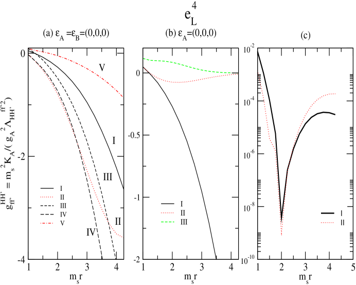
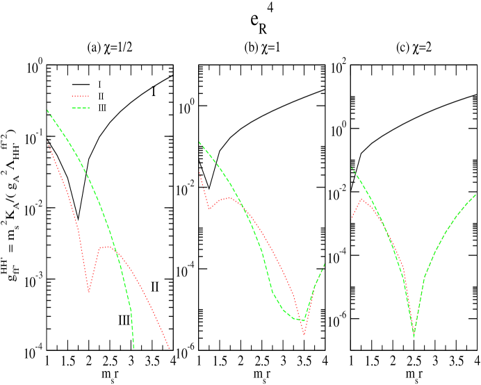
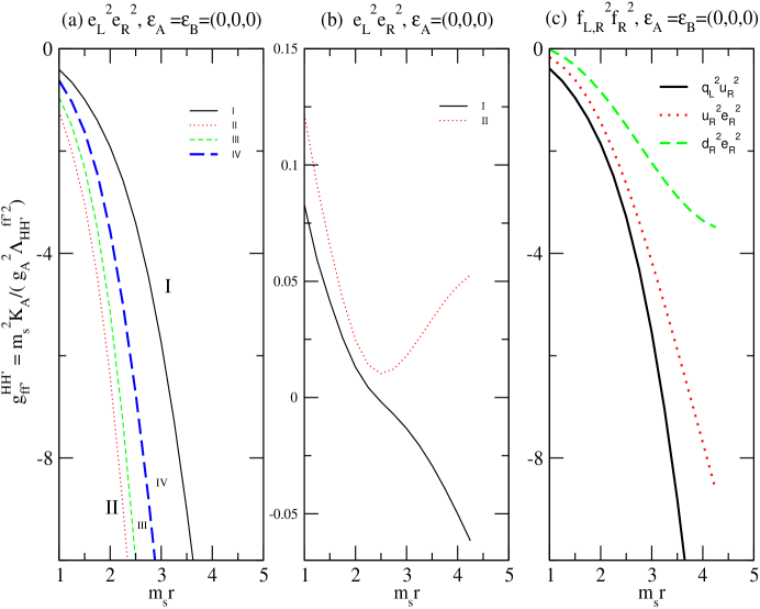
For a clearer assessment of the dependence on msโ€‹rsubscript๐‘š๐‘ ๐‘Ÿm_{s}r, we display in Figuresย 1, 2 and 3 plots of the coefficients $g_{ij,kl}^{HH^{\prime}}$. We study here the sensitivity on the geometric parameters by varying these one by one with respect to the reference set. Note that the longitudinal distances $\epsilon_{A},\ \epsilon_{B}$ are associated with flavor change while the transverse distances are associated with gauge symmetry breaking. We group the configurations into three classes corresponding to the flavor change: ฮ”F=0:ฯตA=ฯตB=0;ฮ”F=1:ฯตA=0,ฯตBโ‰ 0;\Delta F=0:\ \epsilon_{A}=\epsilon_{B}=0;\ \Delta F=1:\ \epsilon_{A}=0,\ \epsilon_{B}\neq 0; and ฮ”โ€‹F=2:ฯตAโ‰ 0,ฯตBโ‰ 0:ฮ”๐น2formulae-sequencesubscriptitalic-ฯต๐ด0subscriptitalic-ฯต๐ต0\Delta F=2:\ \epsilon_{A}\neq 0,\ \epsilon_{B}\neq 0. Figuresย 1 and 2 refer to the unmixed chirality configurations with equal brane angles and Figureย 3 to the mixed chirality configurations with unequal brane angles. The presence of cusp discontinuities in certain curves is due to our use of logarithmic plots for the absolute values of the coefficients aimed at representing quantitatively the size of the suppression.

We see on panel $(a)$ of Fig.ย 1 that the predictions are spread by an approximate factor $2\ -\ 3$ for reasonably restricted variations of the shape parameters. Using tilted 2-d tori, or increasing the complex structure parameter $\chi^{I}$, results in enhanced coefficients, while decreasing $\chi^{I}$ results in reduced coefficients. The $\Delta F=1$ coefficients with finite $\epsilon_{B}$ in panel $(b)$ are suppressed by order $10^{-1}$ while the $\Delta F=2$ coefficients with finite $\epsilon_{A}$ and $\epsilon_{B}$ in panel $(c)$ are suppressed by factors of order $10^{-2}-10^{-4}.$ The specific dependence on msโ€‹rsubscript๐‘š๐‘ ๐‘Ÿm_{s}r is a result of the tension between the power growth from the overall normalization factor gsโˆ(msโ€‹r)3proportional-tosubscript๐‘”๐‘ superscriptsubscript๐‘š๐‘ ๐‘Ÿ3g_{s}\propto(m_{s}r)^{3} and the exponential suppression from $Z_{cl}$. That the suppression effect is controlled by the classical factor is clear from the fact that the coefficients have comparable values near msโ€‹r=1subscript๐‘š๐‘ ๐‘Ÿ1m_{s}r=1.

The plots in Fig.ย 2 again confirm that $\chi^{I}<1$ and $\chi^{I}>1$ lead to reduced and enhanced coefficients. The nearly one order of magnitude suppression of the $\Delta F=1$ coefficients is independent of $\chi^{I}$. That the suppression is weaker than expected is explained by the specific feature in the present model that only a single component of the vectors $\epsilon_{B}^{I}$ are finite. The comparable predictions found for $\epsilon_{B}=(0,1/3,0)$ and $(0,2/3,0)$ are explained by the torus lattice periodicity. The cancellation effects from the oscillating factors $e^{2i\pi\epsilon L}$ explain both the change of sign from positive to negative coefficients and the smooth variation with msโ€‹rsubscript๐‘š๐‘ ๐‘Ÿm_{s}r.

The plots in Fig.ย 3 show that the coefficients in the unequal angle cases are systematically larger than those found for equal angles. The dependence of the wrapped cycle volumes on the torus shape parameters spreads the coefficients by a factor of $2\ -\ 3$.

Two general features of the predictions are the rapid power law increase with msโ€‹rsubscript๐‘š๐‘ ๐‘Ÿm_{s}r of the flavor conserving $\Delta F=0$ coefficients and the hierarchies of order $10^{-1}$ and $10^{-4}$ separating these from the flavor changing $\Delta F=1$ and $\Delta F=2$ coefficients which vary more slowly over the allowed interval for msโ€‹rsubscript๐‘š๐‘ ๐‘Ÿm_{s}r. While the variation of the coefficients with msโ€‹rsubscript๐‘š๐‘ ๐‘Ÿm_{s}r is not apparent on the result in Eq.ย (II.16), obtained by restricting the $x$-integral to the end point contributions, it appears possible to use this approximate formula in order to explain the dependence on the distance parameters, $\epsilon_{A},\ \epsilon_{B}$. Examination of the combined contributions from the string momentum and winding modes to the coefficients

gfโ€‹fโ€ฒHโ€‹Hโ€ฒโ‰ƒ|LA|4โ€‹ฯ€โ€‹|LB|โ€‹โˆ‘pBโ‰ 0โˆ‘pAโˆˆZโˆIฮดIโˆ’|sinโก(ฯ€โ€‹ฮธI)โ€‹(pA+ฯตAI)โ€‹LAI|2+|pB/LBI|2โ€‹e2โ€‹ฯ€โ€‹iโ€‹pBโ€‹ฯตBIโˆ‘I|sinโก(ฯ€โ€‹ฮธI)โ€‹(pA+ฯตAI)โ€‹LAI|2+|pB/LBI|2,similar-to-or-equalssubscriptsuperscript๐‘”๐ปsuperscript๐ปโ€ฒ๐‘“superscript๐‘“โ€ฒsubscript๐ฟ๐ด4๐œ‹subscript๐ฟ๐ตsubscriptsubscript๐‘๐ต0subscriptsubscript๐‘๐ด๐‘subscriptproduct๐ผsuperscriptsubscript๐›ฟ๐ผsuperscript๐œ‹superscript๐œƒ๐ผsubscript๐‘๐ดsuperscriptsubscriptitalic-ฯต๐ด๐ผsuperscriptsubscript๐ฟ๐ด๐ผ2superscriptsubscript๐‘๐ตsuperscriptsubscript๐ฟ๐ต๐ผ2superscript๐‘’2๐œ‹๐‘–subscript๐‘๐ตsuperscriptsubscriptitalic-ฯต๐ต๐ผsubscript๐ผsuperscript๐œ‹superscript๐œƒ๐ผsubscript๐‘๐ดsuperscriptsubscriptitalic-ฯต๐ด๐ผsuperscriptsubscript๐ฟ๐ด๐ผ2superscriptsubscript๐‘๐ตsuperscriptsubscript๐ฟ๐ต๐ผ2\displaystyle g^{HH^{\prime}}_{ff^{\prime}}\simeq{|L_{A}|\over 4\pi|L_{B}|}\sum_{p_{B}\neq 0}\sum_{p_{A}\in Z}{\prod_{I}\delta_{I}^{-|\sin(\pi\theta^{I})(p_{A}+\epsilon_{A}^{I})L_{A}^{I}|^{2}+|p_{B}/L_{B}^{I}|^{2}}e^{2\pi ip_{B}\epsilon_{B}^{I}}\over\sum_{I}|\sin(\pi\theta^{I})(p_{A}+\epsilon_{A}^{I})L_{A}^{I}|^{2}+|p_{B}/L_{B}^{I}|^{2}}, (II.50)

shows that for small finite $\epsilon_{A}$ the leading contribution to the ratio of $\Delta F=1$ to $\Delta F=0$ amplitudes is of form eโˆ’pAโ€‹ฯตAโ€‹|โ„’A|โ€‹(msโ€‹r)2superscript๐‘’subscript๐‘๐ดsubscriptitalic-ฯต๐ดsubscriptโ„’๐ดsuperscriptsubscript๐‘š๐‘ ๐‘Ÿ2e^{-p_{A}\epsilon_{A}|{\cal L}_{A}|(m_{s}r)^{2}}, while the $\Delta F=2$ amplitudes include the additional suppression from the oscillating factors, $e^{2\pi i\epsilon_{B}}$.

It is interesting to compare our predictions for the contact interactions of four fermions with those obtained in the $Dp/D(p+4)$-brane modelsย antbengier01 . (The formalism is briefly reviewed in Appendixย B.) For the coupling of four modes, $|(3,7_{I})|^{2}|(3,7_{J})|^{2}$, the comparison at fixed 4-d gauge coupling constant of our estimate, 2โ€‹ฯ€โ€‹gfโ€‹fโ€ฒHโ€‹Hโ€ฒโ€‹๐’ฎ1234โ€‹๐’ฏ1234โ‰ˆ2โ€‹ฯ€โ€‹(0.05โˆ’ 0.5)โ€‹(msโ€‹r)2โ€‹๐’ฎ1234โ€‹๐’ฏ12342๐œ‹superscriptsubscript๐‘”๐‘“superscript๐‘“โ€ฒ๐ปsuperscript๐ปโ€ฒsubscript๐’ฎ1234subscript๐’ฏ12342๐œ‹0.050.5superscriptsubscript๐‘š๐‘ ๐‘Ÿ2subscript๐’ฎ1234subscript๐’ฏ12342\pi g_{ff^{\prime}}^{HH^{\prime}}{\cal S}_{1234}{\cal T}_{1234}\approx 2\pi(0.05\ -\ 0.5)(m_{s}r)^{2}{\cal S}_{1234}{\cal T}_{1234}, with the result found by Antoniadis et al.,ย antbengier01 in the large radius limit, ${\cal T}_{1234}[0.12\ {\cal P}_{1234}+0.33\ {\cal S}_{1234}]$, reveals an order of magnitude concordance.

Finally, we compare our predictions with the contributions from the momentum modes evaluated by means of Eq.ย (II.24) for $n=3$. The resulting rough estimate, (gfโ€‹fโ€ฒHโ€‹Hโ€ฒ)Kโ€‹Kโ‰ƒ14โ€‹ฯ€โ€‹(nโˆ’2)โ€‹Snโ€‹(msโ€‹r)nโ€‹|โ„’B|โ‰ƒ(msโ€‹r)3โ€‹โ„’Bsimilar-to-or-equalssubscriptsuperscriptsubscript๐‘”๐‘“superscript๐‘“โ€ฒ๐ปsuperscript๐ปโ€ฒ๐พ๐พ14๐œ‹๐‘›2subscript๐‘†๐‘›superscriptsubscript๐‘š๐‘ ๐‘Ÿ๐‘›subscriptโ„’๐ตsimilar-to-or-equalssuperscriptsubscript๐‘š๐‘ ๐‘Ÿ3subscriptโ„’๐ต(g_{ff^{\prime}}^{HH^{\prime}})_{KK}\simeq{1\over 4\pi(n-2)}{S_{n}(m_{s}r)^{n}|{\cal L}_{B}|}\simeq(m_{s}r)^{3}{\cal L}_{B}, indicates that the contributions from the string momentum modes are significantly larger than those from winding modes. We should remember, however, that the present estimate must be regarded as an upper bound since it relies on the large $r$ limit and ignores the form factor suppression.

III Indirect high energy collider tests

We discuss in the present section the collider physics applications based on the formalism presented in Subsectionย II.1 and in Appendixย B for the orientifold model of Cremades et al.,ย CIM ; CIM2 . Since the distinction between the mass and gauge bases is not essential for these observables, all the results in this section are obtained by setting the flavor mixing matrices to unity, $V_{H}^{f}=1$.

III.1 Bounds on contact interactions mass scales

It is important to distinguish the mass scale $\Lambda$ associated to the ${\cal D}=6$ operators from the mass scale $M_{H}$ associated to the ${\cal D}=8$ operators in the 4-d effective Lagrange density quadratic in the energy-momentum tensorย hewett99 , $L_{EFF}=i{4\lambda\over M_{H}^{4}}T_{\mu\nu}T^{\mu\nu}$. The analyses of available high energy collider experimental data using field theories in extra space dimensions are sensitive to values of these mass scales, $M_{H}=1.5$ TeVย hewett99 , $\Lambda=2\ -\ 6$ TeVย rizzo99 and $\Lambda=1\ -\ 8$ TeVย antobequ99 . In the single $Dp$-brane models, the quantum gravity mass scale $M_{H}$ was found to be parametrically larger than the string scaleย cpp00 , MHmsโ‰ƒ23/4ฯ€โ€‹gssimilar-to-or-equalssubscript๐‘€๐ปsubscript๐‘š๐‘ superscript234๐œ‹subscript๐‘”๐‘ {M_{H}\over m_{s}}\simeq{2^{3/4}\over\pi\sqrt{g_{s}}}, thus making the detection of new physics effects harder. To pursue the comparison with the intersecting brane models, it is convenient to consider in place of $M_{H}$ the closely related gravitational mass scale $M_{G}$ defined in the case with $n$ flat extra dimensions byย add99 , $M_{G}^{n+2}r^{n}={M_{P}^{2}\over 4\pi}=(4\pi G_{N})^{-1}$. The mass scale $M_{G}$ is related to the fundamental string parameters of single $D3_{A}$-brane models asย cpp00 , (MG/ms)8=16โ€‹ฯ€/gA4.superscriptsubscript๐‘€๐บsubscript๐‘š๐‘ 816๐œ‹superscriptsubscript๐‘”๐ด4({M_{G}/m_{s}})^{8}={16\pi/g_{A}^{4}}. Repeating the same calculations for intersecting $D6_{A}$-branes gives us the modified formula in the large radius limit

(MGms)8=16โ€‹ฯ€gA4โ€‹(msโ€‹r)6โ€‹|mAIโˆ’nAIโ€‹UI|/U2I.superscriptsubscript๐‘€๐บsubscript๐‘š๐‘ 816๐œ‹superscriptsubscript๐‘”๐ด4superscriptsubscript๐‘š๐‘ ๐‘Ÿ6superscriptsubscript๐‘š๐ด๐ผsuperscriptsubscript๐‘›๐ด๐ผsuperscript๐‘ˆ๐ผsuperscriptsubscript๐‘ˆ2๐ผ\displaystyle({M_{G}\over m_{s}})^{8}={16\pi\over g_{A}^{4}(m_{s}r)^{6}|m_{A}^{I}-n_{A}^{I}U^{I}|/U_{2}^{I}}. (III.1)

The strong dependence on the geometric parameters indicates the interesting possibility that $M_{G}$ may assume lower values in multiple brane models.

We now discuss the constraints on the string mass parameter, mssubscript๐‘š๐‘ m_{s}, inferred by comparing our predictions for the chirality conserving contact interactions of ${\cal D}=6$ with a subset of the available experimental limitsย pdg06 . For the lepton and lepton-quark configurations, $e_{L}^{4},\ e_{L}^{2}q_{L}^{2}$ and the quark configuration, $q_{L}^{4}$, respectively, we evaluate the bounds on the string scale parameter, ms2=giโ€‹i,iโ€‹iLโ€‹Lโ€‹ฮ›Lโ€‹Leโ€‹fโ€‹2โ€‹(1+ฮดeโ€‹f)โ€‹gA2/KAsuperscriptsubscript๐‘š๐‘ 2subscriptsuperscript๐‘”๐ฟ๐ฟ๐‘–๐‘–๐‘–๐‘–subscriptsuperscriptฮ›๐‘’๐‘“2๐ฟ๐ฟ1subscript๐›ฟ๐‘’๐‘“superscriptsubscript๐‘”๐ด2subscript๐พ๐ดm_{s}^{2}=g^{LL}_{ii,ii}\Lambda^{ef2}_{LL}(1+\delta_{ef})g_{A}^{2}/K_{A}, at fixed msโ€‹rsubscript๐‘š๐‘ ๐‘Ÿm_{s}r, by setting the gauge coupling constants, $g_{A}^{2}/K_{A}$ at $g_{2}^{2}/2\simeq 0.213$ and $g_{3}^{2}\simeq 1.44$, respectively. Using the numerical values of the coefficients in Tableย 1, we obtain the following bounds on mssubscript๐‘š๐‘ m_{s} for the choice of three representative experimental limits on the mass scales:

ฮ›Lโ€‹Lยฑโ€‹(eโ€‹eโ€‹eโ€‹e)>[4.7, 6.1]โŸนms>[0.69, 2.1, 3.9]subscriptsuperscriptฮ›plus-or-minus๐ฟ๐ฟ๐‘’๐‘’๐‘’๐‘’4.76.1โŸนsubscript๐‘š๐‘ 0.692.13.9\displaystyle\Lambda^{\pm}_{LL}(eeee)>[4.7,\ 6.1]\ \Longrightarrow\ m_{s}>[0.69,\ 2.1,\ 3.9] (III.2)
ฮ›Lโ€‹Lยฑโ€‹(eโ€‹eโ€‹qโ€‹q)>[23.3, 12.5]โŸนms>[2.4, 3.0, 5.6]subscriptsuperscriptฮ›plus-or-minus๐ฟ๐ฟ๐‘’๐‘’๐‘ž๐‘ž23.312.5โŸนsubscript๐‘š๐‘ 2.43.05.6\displaystyle\Lambda^{\pm}_{LL}(eeqq)>[23.3,\ 12.5]\ \Longrightarrow\ m_{s}>[2.4,\ 3.0,\ 5.6] (III.3)
ฮ›Lโ€‹Lยฑโ€‹(qโ€‹qโ€‹qโ€‹q)>[2.7]โŸนms>[0.72, 1.7, 3.2],subscriptsuperscriptฮ›plus-or-minus๐ฟ๐ฟ๐‘ž๐‘ž๐‘ž๐‘ždelimited-[]2.7โŸนsubscript๐‘š๐‘ 0.721.73.2\displaystyle\Lambda^{\pm}_{LL}(qqqq)>[2.7]\ \Longrightarrow\ m_{s}>[0.72,\ 1.7,\ 3.2], (III.4)

where all masses are expressed in TeV units and the three entries refer to the values msโ€‹r=[1, 2, 3]subscript๐‘š๐‘ ๐‘Ÿ123m_{s}r=[1,\ 2,\ 3].

We next consider the constraint from the enhanced supernova cooling through the reaction producing right handed neutrino-antineutrino pairs by quark-antiquark pairs, $q+\bar{q}\to\nu^{c}+\bar{\nu}^{c}$, which is allowed as long as the contributions to the neutrino Dirac mass are bounded by the supernova temperature, $m_{\nu}\leq T_{SN}\simeq 50$ MeV. The lower bound on the mass scale in the effective Lagrangian, $L_{EFF}={4\pi\over\Lambda^{q\nu_{R}2}}(\bar{q}\gamma_{\mu}\gamma_{5}q)(\bar{\nu}_{R}\gamma^{\mu}\nu_{R})$, is found for the SN1987A to cover the rangeย grifols98 , $\Lambda^{q\nu_{R}}>(90\ -\ 250)$ TeV. For concreteness, we set our choice on the lower bound, $\Lambda^{q\nu_{R}}>200$ TeV. Using the numerical predictions in Tableย 1 and assuming the approximate equalities between the chirality basis amplitudes, $q_{L}^{2}\nu_{R}^{2}\simeq q_{L}^{2}u_{R}^{2}$ and $d_{R}^{2}\nu_{R}^{2}\simeq d_{R}^{4}$, we obtain the numerical estimate for the coefficient, $(g^{LR}_{q_{L}\nu_{R}}+g^{RR}_{q_{R}\nu_{R}})\simeq[0.66,\ 1.26,\ 2.14]$ for msโ€‹r=[1, 2, 3]subscript๐‘š๐‘ ๐‘Ÿ123m_{s}r=[1,\ 2,\ 3]. The resulting bounds on the string mass scale read, ms>[43, 82, 139]subscript๐‘š๐‘ 4382139m_{s}>[43,\ 82,\ 139] TeV. For reference, we note that the comparison with the contribution from the string momentum modes yieldsย abeleb03 the weaker bound, msโ‰ฅ(5โˆ’ 10)subscript๐‘š๐‘ 510m_{s}\geq(5\ -\ 10) TeV.

III.2 Bhabha scattering cross section

Useful constraints on the new physics are set by the experimental data at the high-energy colliders involving the two-body processesย lep2rev of Bhabha, Mรถller and photon pair scattering and fermion-antifermion pair production. The absence of significant deviations from the Standard Model predictions has led the statistical analyses of data to set exclusion limits on the free parameters. The global fits to the combined high-energy collider data based on the single $D$-brane model, with the gauge factors treated as free parameters, yieldsย cheung05 ms>(0.69โˆ’ 1.96)subscript๐‘š๐‘ 0.691.96m_{s}>(0.69\ -\ 1.96) TeV.

We focus here on the Bhabha scattering differential cross section for which high precision measurements along with higher order calculations of the pertubation theory corrections are due in the future. Experimental data has been collected by the LEP collaborationsย l399 ; aleph99 ; opal99 . The studies based on single $Dp$-brane models, describing the ratio of the string to Standard Model differential cross sections by the approximate formulaย cpp00

Rโ€‹(cosโกฮธ)โ‰ก(dโ€‹ฯƒ/dโ€‹ฮฉ)(dโ€‹ฯƒ/dโ€‹ฮฉ)Sโ€‹M=|๐’ฎโ€‹(s,t)|2,๐‘…๐œƒ๐‘‘๐œŽ๐‘‘ฮฉsubscript๐‘‘๐œŽ๐‘‘ฮฉ๐‘†๐‘€superscript๐’ฎ๐‘ ๐‘ก2\displaystyle R(\cos\theta)\equiv{(d\sigma/d\Omega)\over(d\sigma/d\Omega)_{SM}}=|{\cal S}(s,t)|^{2}, (III.5)
[๐’ฎโ€‹(s,t)โ‰กฮ“โ€‹(1โˆ’s)โ€‹ฮ“โ€‹(1โˆ’t)ฮ“โ€‹(1โˆ’sโˆ’t)โ‰ƒ1โˆ’ฯ€2โ€‹sโ€‹t6โ€‹ms4+โ‹ฏ]delimited-[]๐’ฎ๐‘ ๐‘กฮ“1๐‘ ฮ“1๐‘กฮ“1๐‘ ๐‘กsimilar-to-or-equals1superscript๐œ‹2๐‘ ๐‘ก6superscriptsubscript๐‘š๐‘ 4โ‹ฏ\displaystyle[{\cal S}(s,t)\equiv{\Gamma(1-s)\Gamma(1-t)\over\Gamma(1-s-t)}\simeq 1-{\pi^{2}st\over 6m_{s}^{4}}+\cdots] (III.6)

yield by comparison with the experimental data at the center of mass energy s=183๐‘ 183\sqrt{s}=183 GeV the $95\%$ confidence level exclusion limit on the string mass scale, ms>410subscript๐‘š๐‘ 410m_{s}>410 GeV. Similar bounds are found in the analysisย bouril99 including the experimental data at s=188.7๐‘ 188.7\sqrt{s}=188.7 GeV. At the higher energy, s=1๐‘ 1\sqrt{s}=1 TeV, the $95\%$ confidence exclusion limit obtained under similar conditions should extend the sensitivity reach toย cpp00 , ms>3.1subscript๐‘š๐‘ 3.1m_{s}>3.1 TeV.

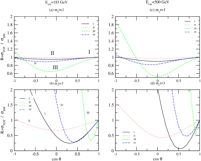
We now present our predictions for the Bhabha scattering differential cross section evaluated with Cremades et al.,ย CIM ; CIM2 model by adding the contributions from the contact interactions in Eq.ย (II.23) to the Standard Model amplitudes, using the formalism detailed in Appendixย B.2. In Fig.ย 4 and Fig.ย 5, we show plots of the ratio $R(\cos\theta)$ as a function of the scattering angle variable, $\cos\theta$, for the center of mass energies, s=183๐‘ 183\sqrt{s}=183 GeV and s=500๐‘ 500\sqrt{s}=500 GeV, respectively. The selected set of values for mssubscript๐‘š๐‘ m_{s} are different for these two cases, as dictated by the fact that the string corrections scale as s/ms2๐‘ superscriptsubscript๐‘š๐‘ 2s/m_{s}^{2}.

For a qualitative comparison with experimental data, we note that the LEP data points for the ratio at s=0.183๐‘ 0.183\sqrt{s}=0.183 TeV are spread over the interval of $\cos\theta\in[-1,\ +1]$ inside the band limited by the horizontal lines at, $R(\cos\theta)=(1.0\pm 0.4)$. As for the single $D$-brane model predictionย cpp00 in Eq.(III.6), this is represented by a nearly straight line which slopes from $1.06$ to $1.0$ as $\cos\theta$ increases from $-1$ to $1$. The exchange of string Regge and winding modes are seen to give a small reduction of $R(\cos\theta)$ near the forward scattering angles, $\cos\theta\sim 1$, gradually turning into a large enhancement near the backward angles, $\cos\theta\sim-1$. This implies a change from a relative negative sign to a positive sign at some intermediate angle in the interval $\cos\theta\in[-1,\ +1]$. The contributions grow rapidly with increasing msโ€‹rsubscript๐‘š๐‘ ๐‘Ÿm_{s}r. Requiring the predicted ratios in Figs.ย 4 andย 5 to remain bounded inside the interval $R(\cos\theta)\in[0.8,1.2]$ for $\cos\theta\in[-1,\ +1]$ imposes lower bounds on the string scale which cover the ranges, $m_{s}\geq(0.5\ -\ 3.)$ TeV and $m_{s}\geq(2.\ -\ 5.)$ TeV, respectively, for the interval of values msโ€‹rโˆˆ[1,3]subscript๐‘š๐‘ ๐‘Ÿ13m_{s}r\in[1,3].

We have also performed a more realistic calculation of the Bhabha scattering differential cross section in which the total regularized string amplitudes are obtained by subtracting by hand the pole terms from exchange of massless and massive momentum modes for the $\gamma\ +Z$ gauge bosons, while adding up the contributions from the physical $\gamma\ +Z$ pole terms, using the prescription in Eq.ย (II.23). To ease the numerical calculations we have only evaluated the pure chirality amplitudes $LL,\ RR$, while assuming the mixed chirality amplitudes $LR,\ RL$ to be proportional to these. The model dependence on the ratio of pure to mixed chirality amplitudes thus resides in the adjustable proportionality constant, $x=G_{e^{c}_{L}e_{L}}/G_{e_{L}e_{L}}=G^{RL}/G^{LL}=G^{LR}/G^{LL}$, which we have taken to vary inside the interval, $x=[{1\over 2},\ 5].$

The ratio $R(\cos\theta)$ of the predicted differential cross section to that of the Standard Model is plotted in Fig.ย 6 at the center of mass energies, s=183๐‘ 183\sqrt{s}=183 and $500$ GeV (left and right hand panels) for the two values of the string scale, ms=1, 2subscript๐‘š๐‘ 12m_{s}=1,\ 2 TeV and ms=2, 4subscript๐‘š๐‘ 24m_{s}=2,\ 4 TeV, respectively. The comparison of the curves $I,\ II$, and similarly of the curves $III,\ IV$, measures the sensitivity of $R(\cos\theta)$ with respect to the string scale mssubscript๐‘š๐‘ m_{s}. On the other hand, the comparison of the curves $I,\ III$, and similarly of the curves $II,\ IV$, measures the sensitivity with respect to the mixed chirality amplitudes. The large spread of predictions with variable $x$ and mssubscript๐‘š๐‘ m_{s} shows that Bhabha scattering can usefully test the model dependence. The results from the present complete calculation agree qualitatively with those in Figs.ย 4 andย 5, although the change of slope and subsequent rise of the ratio with decreasing $\cos\theta$ are generally less steep. We conclude that the representation of string amplitudes by contact interactions is reliable for the considered incident energies.

IV Flavor changing neutral current processes

IV.1 Direct and indirect flavor changing effects

The flavor changing neutral current observables are determined by the non-diagonal elements of the mass basis coefficients of contact interactions, $\tilde{G}_{ij,kl}$. These receive direct flavor changing contributions from the four point string amplitudes and indirect contributions from the linear transformations linking the gauge and mass bases of the fermions. Without further input information on the flavor structure, it appears impossible to infer quantitative constraints from a comparison with the flavor changing observables.

A natural description of the fermions flavor quantum numbers is provided by the basis labeled by the branes intersection points. The geometric constraints on string amplitudes, as stated by Eq.ย (II.33), directly translate as selection rules on the flavor amplitudes in this basis. For Cremades et al.,ย CIM ; CIM2 model, however, these rules turn out to be trivial ones, owing to the fact that the intersection points for the fixed chirality modes lie at finite distances apart only in single complex planes. Since the conditions involve at least one shift vector defined modulo $1$, no zero entries are enforced either on the trilinear Yukawa interactions, $\lambda^{f}_{ij}f_{i}f^{c}_{j}H$, or on the four fermions interactions, $G_{ij,kl}\bar{f}_{i}f_{j}\bar{f}_{k}f_{l}$. This property is also responsible for the separable structure of the Yukawa coupling constants, $\lambda^{f}_{ij}=a_{i}b_{j}$, implying that the mass matrices of quarks and leptons all have unit rank. Although the flavor non-diagonal coefficients are generally finite, the $\Delta F=1,\ 2$ operators associated with the configurations, i=jโ‰ k=l๐‘–๐‘—๐‘˜๐‘™i=j\neq k=l and iโ‰ jโ‰ k๐‘–๐‘—๐‘˜i\neq j\neq k, are strongly suppressed with increasing msโ€‹rsubscript๐‘š๐‘ ๐‘Ÿm_{s}r by the classical partition function factor for longitudinal distance parameters, $\epsilon_{A},\ \epsilon_{B}$ of $O(1)$. However, the fact that the tree level string amplitudes depend on the relative distances between intersection points, $\epsilon^{A}_{ij}$ and $\epsilon^{B}_{jk}$, introduces certain restrictions on the flavor structure of the coefficients $G_{ij,kl}$.

We here focus on the two flavor changing neutral current observables associated to the mass splitting of CP conjugate pairs of neutral mesons made of quark-antiquark pairs, $P=q_{i}\bar{q}_{j},\ \bar{P}=\bar{q}_{i}q_{j}$, and the three-body decays of leptons, $l_{j}\to l_{i}+l_{k}+\bar{l}_{l}.$ For simplicity, we assume that the Standard Model contributions to these observables are negligible relative to those from the contact interactions, so that we can directly use the experimental limit to derive bounds on the string scale. Convenient formulas for the contributions to these observables from the chirality conserving local operators have been obtained inย langplum00 for models with extra $U(1)$ gauge symmetries. We follow closely the formalism developed in the latter work, while accounting for the fact that the dependence on the color quantum numbers is different in our case. The observables for the real and imaginary parts of the $P^{0}-\bar{P}^{0}$ mass splitting, $\Delta m_{P}\equiv-\Re(<P_{0}|L^{DS=2}_{EFF}|\bar{P}^{0}>)$ and $\epsilon_{P}\equiv-\Im(<P_{0}|L^{DS=2}_{EFF}|\bar{P}^{0}>)/(2\sqrt{2}m_{P})$, are given in our notations by the explicit formulas

$\displaystyle\Delta m_{P}=-2m_{P}F_{P}^{2}[{1\over 3}\Re(\tilde{G}^{LL}_{ij,ij}+\tilde{G}^{RR}_{ij,ij})-\alpha^{\prime}_{ij}\Re(\tilde{G}^{LR}_{ij,ij})],$ (IV.1)
$\displaystyle\epsilon_{P}={m_{P}F_{P}^{2}\over\sqrt{2}\Delta m_{P}}[{1\over 3}\Im(\tilde{G}^{LL}_{ij,ij}+\tilde{G}^{RR}_{ij,ij})-\alpha^{\prime}_{ij}\Im(\tilde{G}^{LR}_{ij,ij})],$ (IV.2)

where $\alpha^{\prime}_{ij}={1\over 3}+{2\over 3}({m_{P}\over m_{q_{i}}+m_{q_{j}}})^{2}$. Note that the definition for the indirect CP violation observable applies specifically to the $K-\bar{K}$ system, $\epsilon_{P}=\epsilon_{K}$. The quarks flavor indices $i,\ j$ are set in accordance with the conventional assignments for the neutral mesons, K0โ€‹(sยฏโ€‹d),B0โ€‹(bยฏโ€‹d),Bs0โ€‹(bยฏโ€‹s),D0โ€‹(uยฏโ€‹c),superscript๐พ0ยฏ๐‘ ๐‘‘superscript๐ต0ยฏ๐‘๐‘‘superscriptsubscript๐ต๐‘ 0ยฏ๐‘๐‘ superscript๐ท0ยฏ๐‘ข๐‘K^{0}(\bar{s}d),\ B^{0}(\bar{b}d),\ B_{s}^{0}(\bar{b}s),\ D^{0}(\bar{u}c), with $F_{P}$ denoting the mesons two-body leptonic decay coupling constants. We have evaluated the hadronic matrix elements of the four fermion local operators for the pseudoscalar mesons to vacuum transition by making use of the vacuum insertion approximation. The bilinear axial current hadronic matrix elements are determined through the PCAC hypothesis in terms of the measured parameters $F_{P}$. Using the conventional definitions for the matrix elements of quark bilinear current operators

<0|sยฏฮฑโ€‹Lโ€‹ฮณฮผโ€‹dฮฒโ€‹L|K0โ€‹(p)>=โˆ’<Kยฏ0โ€‹(p)|sยฏฮฑโ€‹Lโ€‹ฮณฮผโ€‹dฮฒโ€‹L|0>=iโ€‹FK6โ€‹2โ€‹mKโ€‹pฮผโ€‹ฮดaโ€‹ฮฒ,quantum-operator-product0subscriptยฏ๐‘ ๐›ผ๐ฟsuperscript๐›พ๐œ‡subscript๐‘‘๐›ฝ๐ฟsuperscript๐พ0๐‘quantum-operator-productsuperscriptยฏ๐พ0๐‘subscriptยฏ๐‘ ๐›ผ๐ฟsuperscript๐›พ๐œ‡subscript๐‘‘๐›ฝ๐ฟ0๐‘–subscript๐น๐พ62subscript๐‘š๐พsuperscript๐‘๐œ‡subscript๐›ฟ๐‘Ž๐›ฝ\displaystyle<0|\bar{s}_{\alpha L}\gamma^{\mu}d_{\beta L}|K^{0}(p)>=-<\bar{K}^{0}(p)|\bar{s}_{\alpha L}\gamma^{\mu}d_{\beta L}|0>=i{F_{K}\over 6\sqrt{2m_{K}}}p^{\mu}\delta_{a\beta}, (IV.3)
<0|sยฏฮฑโ€‹ฮณ5โ€‹dฮฒ|K0โ€‹(p)>=<Kยฏ0โ€‹(p)|sยฏฮฑโ€‹ฮณ5โ€‹dฮฒ|0>=โˆ’iโ€‹FKโ€‹mK23โ€‹2โ€‹mKโ€‹(ms+md)โ€‹ฮดaโ€‹ฮฒ,quantum-operator-product0subscriptยฏ๐‘ ๐›ผsubscript๐›พ5subscript๐‘‘๐›ฝsuperscript๐พ0๐‘quantum-operator-productsuperscriptยฏ๐พ0๐‘subscriptยฏ๐‘ ๐›ผsubscript๐›พ5subscript๐‘‘๐›ฝ0๐‘–subscript๐น๐พsuperscriptsubscript๐‘š๐พ232subscript๐‘š๐พsubscript๐‘š๐‘ subscript๐‘š๐‘‘subscript๐›ฟ๐‘Ž๐›ฝ\displaystyle<0|\bar{s}_{\alpha}\gamma_{5}d_{\beta}|K^{0}(p)>=<\bar{K}^{0}(p)|\bar{s}_{\alpha}\gamma_{5}d_{\beta}|0>=-i{F_{K}m_{K}^{2}\over 3\sqrt{2m_{K}}(m_{s}+m_{d})}\delta_{a\beta}, (IV.4)

one can write the matrix elements of the relevant quadratic operators as

Qฮฑโ€‹ฮฒโ€‹ฮณโ€‹ฮดLโ€‹Lโ‰ก<Kยฏ0|(sยฏฮฑโ€‹Lโ€‹ฮณฮผโ€‹dฮฒโ€‹L)โ€‹(sยฏฮณโ€‹Lโ€‹ฮณฮผโ€‹dฮดโ€‹L)|K0>=FK2โ€‹mK36โ€‹(ฮดฮฑโ€‹ฮฒโ€‹ฮดฮณโ€‹ฮด+ฮดฮฑโ€‹ฮดโ€‹ฮดฮณโ€‹ฮฒ),subscriptsuperscript๐‘„๐ฟ๐ฟ๐›ผ๐›ฝ๐›พ๐›ฟquantum-operator-productsuperscriptยฏ๐พ0subscriptยฏ๐‘ ๐›ผ๐ฟsuperscript๐›พ๐œ‡subscript๐‘‘๐›ฝ๐ฟsubscriptยฏ๐‘ ๐›พ๐ฟsuperscript๐›พ๐œ‡subscript๐‘‘๐›ฟ๐ฟsuperscript๐พ0superscriptsubscript๐น๐พ2subscript๐‘š๐พ36subscript๐›ฟ๐›ผ๐›ฝsubscript๐›ฟ๐›พ๐›ฟsubscript๐›ฟ๐›ผ๐›ฟsubscript๐›ฟ๐›พ๐›ฝ\displaystyle Q^{LL}_{\alpha\beta\gamma\delta}\equiv<\bar{K}^{0}|(\bar{s}_{\alpha L}\gamma^{\mu}d_{\beta L})(\bar{s}_{\gamma L}\gamma^{\mu}d_{\delta L})|K^{0}>={F_{K}^{2}m_{K}\over 36}(\delta_{\alpha\beta}\delta_{\gamma\delta}+\delta_{\alpha\delta}\delta_{\gamma\beta}), (IV.5)
Qฮฑโ€‹ฮฒโ€‹ฮณโ€‹ฮดLโ€‹Rโ‰ก<Kยฏ0|(sยฏฮฑโ€‹Lโ€‹ฮณฮผโ€‹dฮฒโ€‹L)โ€‹(sยฏฮณโ€‹Rโ€‹ฮณฮผโ€‹dฮดโ€‹R)|K0>=โˆ’FK2โ€‹mK36โ€‹[ฮดฮฑโ€‹ฮฒโ€‹ฮดฮณโ€‹ฮด+2โ€‹(mKmqi+mqj)2โ€‹ฮดฮฑโ€‹ฮดโ€‹ฮดฮณโ€‹ฮฒ],subscriptsuperscript๐‘„๐ฟ๐‘…๐›ผ๐›ฝ๐›พ๐›ฟquantum-operator-productsuperscriptยฏ๐พ0subscriptยฏ๐‘ ๐›ผ๐ฟsuperscript๐›พ๐œ‡subscript๐‘‘๐›ฝ๐ฟsubscriptยฏ๐‘ ๐›พ๐‘…superscript๐›พ๐œ‡subscript๐‘‘๐›ฟ๐‘…superscript๐พ0superscriptsubscript๐น๐พ2subscript๐‘š๐พ36delimited-[]subscript๐›ฟ๐›ผ๐›ฝsubscript๐›ฟ๐›พ๐›ฟ2superscriptsubscript๐‘š๐พsubscript๐‘šsubscript๐‘ž๐‘–subscript๐‘šsubscript๐‘ž๐‘—2subscript๐›ฟ๐›ผ๐›ฟsubscript๐›ฟ๐›พ๐›ฝ\displaystyle Q^{LR}_{\alpha\beta\gamma\delta}\equiv<\bar{K}^{0}|(\bar{s}_{\alpha L}\gamma^{\mu}d_{\beta L})(\bar{s}_{\gamma R}\gamma^{\mu}d_{\delta R})|K^{0}>=-{F_{K}^{2}m_{K}\over 36}[\delta_{\alpha\beta}\delta_{\gamma\delta}+2({m_{K}\over m_{q_{i}}+m_{q_{j}}})^{2}\delta_{\alpha\delta}\delta_{\gamma\beta}], (IV.6)
โŸนQฮฑโ€‹ฮฒโ€‹ฮณโ€‹ฮดLโ€‹Lโ€‹Tฮฑโ€‹ฮฒโ€‹ฮณโ€‹ฮด=FK2โ€‹mK3,Qฮฑโ€‹ฮฒโ€‹ฮณโ€‹ฮดLโ€‹Rโ€‹Tฮฑโ€‹ฮฒโ€‹ฮณโ€‹ฮด=โˆ’FK2โ€‹mK3โ€‹[1+2โ€‹(mKms+md)2],formulae-sequenceโŸนabsentsubscriptsuperscript๐‘„๐ฟ๐ฟ๐›ผ๐›ฝ๐›พ๐›ฟsubscript๐‘‡๐›ผ๐›ฝ๐›พ๐›ฟsuperscriptsubscript๐น๐พ2subscript๐‘š๐พ3subscriptsuperscript๐‘„๐ฟ๐‘…๐›ผ๐›ฝ๐›พ๐›ฟsubscript๐‘‡๐›ผ๐›ฝ๐›พ๐›ฟsuperscriptsubscript๐น๐พ2subscript๐‘š๐พ3delimited-[]12superscriptsubscript๐‘š๐พsubscript๐‘š๐‘ subscript๐‘š๐‘‘2\displaystyle\ \Longrightarrow\ Q^{LL}_{\alpha\beta\gamma\delta}T_{\alpha\beta\gamma\delta}={F_{K}^{2}m_{K}\over 3},\ Q^{LR}_{\alpha\beta\gamma\delta}T_{\alpha\beta\gamma\delta}=-{F_{K}^{2}m_{K}\over 3}[1+2({m_{K}\over m_{s}+m_{d}})^{2}], (IV.7)

where the saturation of color indices displayed in the last entry above uses the tensor, $T_{\alpha\beta\gamma\delta}={1\over 2}(\delta_{\alpha\beta}\delta_{\gamma\delta}+\delta_{\alpha\delta}\delta_{\gamma\beta})$. The factor $\alpha^{\prime}_{ij}$ accompanying the coefficient $\tilde{G}^{LR}_{ij,ij}$, differs from that quoted inย langplum00 , $\alpha_{ij}={1\over 2}+{1\over 3}({m_{P}\over m_{q_{i}}+m_{q_{j}}})^{2}$, which refers to the dependence on color indices involving the diagonal tensor, $\delta_{\alpha\beta}\delta_{\gamma\delta}$. Similar formulas hold for the $B$ and $D$ mesons.

The contributions from contact interactions to the lepton number violating three-body decay rates of charged leptons are given byย langplum00

$\displaystyle\Gamma(e_{j}\to e_{i}+e_{k}+\bar{e}_{l})={m_{e_{j}}^{5}\over 384\pi^{3}}[(|\tilde{G}^{LL}_{ji,kl}|^{2}+|\tilde{G}^{LL}_{ji,kl}|^{2}+|\tilde{G}^{LR}_{ji,kl}|^{2}+|\tilde{G}^{LR}_{ji,kl}|^{2})+(L\leftrightarrow R)].$ (IV.8)

The partial rates for the pair of decay reactions, $\mu^{-}\to e^{-}+e^{+}+e^{-}$ and $\tau^{-}\to e^{-}+e^{+}+e^{-},$ with $j=2,\ 3$ and $i=k=l=1$, are described by the simplified formula

ฮ“โ€‹(ejโ†’ei+ei+eยฏi)=mej5384โ€‹ฯ€3โ€‹(2โ€‹ฯ€โ€‹gA2ms2โ€‹KA)2โ€‹[2โ€‹|g~jโ€‹i,iโ€‹iLโ€‹L|2+2โ€‹|g~jโ€‹i,iโ€‹iRโ€‹R|2+|g~jโ€‹i,iโ€‹iLโ€‹R|2+|g~jโ€‹i,iโ€‹iRโ€‹L|2],ฮ“โ†’subscript๐‘’๐‘—subscript๐‘’๐‘–subscript๐‘’๐‘–subscriptยฏ๐‘’๐‘–superscriptsubscript๐‘šsubscript๐‘’๐‘—5384superscript๐œ‹3superscript2๐œ‹superscriptsubscript๐‘”๐ด2superscriptsubscript๐‘š๐‘ 2subscript๐พ๐ด2delimited-[]2superscriptsubscriptsuperscript~๐‘”๐ฟ๐ฟ๐‘—๐‘–๐‘–๐‘–22superscriptsubscriptsuperscript~๐‘”๐‘…๐‘…๐‘—๐‘–๐‘–๐‘–2superscriptsubscriptsuperscript~๐‘”๐ฟ๐‘…๐‘—๐‘–๐‘–๐‘–2superscriptsubscriptsuperscript~๐‘”๐‘…๐ฟ๐‘—๐‘–๐‘–๐‘–2\displaystyle\Gamma(e_{j}\to e_{i}+e_{i}+\bar{e}_{i})={m_{e_{j}}^{5}\over 384\pi^{3}}({2\pi g_{A}^{2}\over m_{s}^{2}K_{A}})^{2}[2|\tilde{g}^{LL}_{ji,ii}|^{2}+2|\tilde{g}^{RR}_{ji,ii}|^{2}+|\tilde{g}^{LR}_{ji,ii}|^{2}+|\tilde{g}^{RL}_{ji,ii}|^{2}], (IV.9)

where we have included an extra symmetry factor ${1\over 2}$ in order to account for the pair of identical charged leptons in the final states.

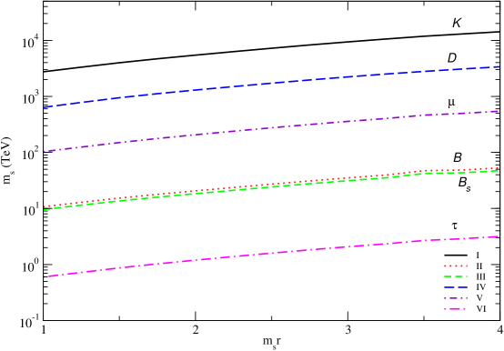
The bounds on the string scale implied by the mesons mass shifts and the charged leptons decay rates are expressed by the explicit formulas

msโ‰ฅ[โˆ’2โ€‹ฯ€โ€‹gA2KAโ€‹2โ€‹mPโ€‹FP2ฮ”โ€‹mPโ€‹[13โ€‹โ„œโก(g~iโ€‹j,iโ€‹jLโ€‹L+g~iโ€‹j,iโ€‹jRโ€‹R)โˆ’ฮฑiโ€‹jโ€ฒโ€‹โ„œโก(g~iโ€‹j,iโ€‹jLโ€‹R)]]12,subscript๐‘š๐‘ superscriptdelimited-[]2๐œ‹superscriptsubscript๐‘”๐ด2subscript๐พ๐ด2subscript๐‘š๐‘ƒsuperscriptsubscript๐น๐‘ƒ2ฮ”subscript๐‘š๐‘ƒdelimited-[]13subscriptsuperscript~๐‘”๐ฟ๐ฟ๐‘–๐‘—๐‘–๐‘—subscriptsuperscript~๐‘”๐‘…๐‘…๐‘–๐‘—๐‘–๐‘—subscriptsuperscript๐›ผโ€ฒ๐‘–๐‘—subscriptsuperscript~๐‘”๐ฟ๐‘…๐‘–๐‘—๐‘–๐‘—12\displaystyle m_{s}\geq\bigg{[}-{2\pi g_{A}^{2}\over K_{A}}{2m_{P}F_{P}^{2}\over\Delta m_{P}}[{1\over 3}\Re(\tilde{g}^{LL}_{ij,ij}+\tilde{g}^{RR}_{ij,ij})-\alpha^{\prime}_{ij}\Re(\tilde{g}^{LR}_{ij,ij})]\bigg{]}^{1\over 2}, (IV.10)
msโ‰ฅ(2โ€‹ฯ€โ€‹gA2KA)12โ€‹[mj5384โ€‹ฯ€3โ€‹ฮ“โ€‹(ejโ†’ei+ei+eยฏi)โ€‹(2โ€‹|g~jโ€‹i,iโ€‹iLโ€‹L|2+2โ€‹|g~jโ€‹i,iโ€‹iRโ€‹R|2+2โ€‹|g~jโ€‹i,iโ€‹iLโ€‹R|2+2โ€‹|g~jโ€‹i,iโ€‹iRโ€‹L|2)]1/4.subscript๐‘š๐‘ superscript2๐œ‹superscriptsubscript๐‘”๐ด2subscript๐พ๐ด12superscriptdelimited-[]superscriptsubscript๐‘š๐‘—5384superscript๐œ‹3ฮ“โ†’subscript๐‘’๐‘—subscript๐‘’๐‘–subscript๐‘’๐‘–subscriptยฏ๐‘’๐‘–2superscriptsubscriptsuperscript~๐‘”๐ฟ๐ฟ๐‘—๐‘–๐‘–๐‘–22superscriptsubscriptsuperscript~๐‘”๐‘…๐‘…๐‘—๐‘–๐‘–๐‘–22superscriptsubscriptsuperscript~๐‘”๐ฟ๐‘…๐‘—๐‘–๐‘–๐‘–22superscriptsubscriptsuperscript~๐‘”๐‘…๐ฟ๐‘—๐‘–๐‘–๐‘–214\displaystyle m_{s}\geq({2\pi g_{A}^{2}\over K_{A}})^{1\over 2}\bigg{[}{m_{j}^{5}\over 384\pi^{3}\Gamma(e_{j}\to e_{i}+e_{i}+\bar{e}_{i})}(2|\tilde{g}^{LL}_{ji,ii}|^{2}+2|\tilde{g}^{RR}_{ji,ii}|^{2}+2|\tilde{g}^{LR}_{ji,ii}|^{2}+2|\tilde{g}^{RL}_{ji,ii}|^{2})\bigg{]}^{1/4}. (IV.11)

In view of the partial information that we dispose on the matrices $V^{f}_{H}$ and the complicated summations over the flavor basis amplitudes, we choose to perform an approximate calculation motivated by the specific flavor structure of contact interactions for the model at hand. We only retain the coefficients $g_{ij,kl}^{HH^{\prime}}$ with $i=j,\ k=l$, denoted by $g^{HH^{\prime}}_{ik}\equiv g^{HH^{\prime}}_{ii,kk}$, and neglect the distinction between intersection points, by assuming the diagonal terms $g_{ii}$ to be independent of $i$ and the non-diagonal terms to be symmetric, $g_{ij}=g_{ji}$. Applying now the unitarity conditions on the quarks transformation matrices, $V^{q}_{H}$, allows us to express the mass basis coefficients for the neutral meson observables in the form

$\displaystyle\tilde{g}^{HH^{\prime}}_{ij,ij}\simeq(2h_{ij}h^{{}^{\prime}}_{ij}+\tilde{h}_{ij}h^{\prime}_{ij}+h_{ij}\tilde{h}^{{}^{\prime}}_{ij})(g^{HH^{\prime}}_{ii}-g^{HH^{\prime}}_{ik})+2\tilde{h}_{ij}\tilde{h}^{{}^{\prime}}_{ij}(g^{HH^{\prime}}_{ii}-g^{HH^{\prime}}_{jk})+(\tilde{h}_{ij}h^{\prime}_{ij}+h_{ij}\tilde{h}^{{}^{\prime}}_{ij})(g^{HH^{\prime}}_{ij}-g^{HH^{\prime}}_{jk}),$ (IV.12)
[hiโ€‹j=VHโ€‹iโ€‹jqโ€‹VHโ€‹iโ€‹iqโฃโ‹†,h~iโ€‹j=VHโ€‹iโ€‹jqโฃโ‹†โ€‹VHโ€‹jโ€‹jq,iโ‰ jโ‰ k]delimited-[]formulae-sequencesubscriptโ„Ž๐‘–๐‘—subscriptsuperscript๐‘‰๐‘ž๐ป๐‘–๐‘—subscriptsuperscript๐‘‰๐‘žโ‹†๐ป๐‘–๐‘–formulae-sequencesubscript~โ„Ž๐‘–๐‘—subscriptsuperscript๐‘‰๐‘žโ‹†๐ป๐‘–๐‘—subscriptsuperscript๐‘‰๐‘ž๐ป๐‘—๐‘—๐‘–๐‘—๐‘˜\displaystyle[h_{ij}=V^{q}_{Hij}V^{q\star}_{Hii},\ \tilde{h}_{ij}=V^{q\star}_{Hij}V^{q}_{Hjj},\ i\neq j\neq k] (IV.13)

where $h^{\prime}_{ij},\ \tilde{h}^{\prime}_{ij}$ are given by same formulas as $h_{ij},\ \tilde{h}_{ij}$ with $H\to H^{\prime}$. Assuming further that the non-diagonal elements are independent of the specific pair, $i,j$, so that $g_{12}=g_{13}=g_{23}$, leads to the factorized form

$\displaystyle\tilde{g}^{HH^{\prime}}_{ij,ij}\approx{\cal V}^{P}_{ij}(g^{HH^{\prime}}_{ii}-g^{HH^{\prime}}_{ij}),$ (IV.14)
$\displaystyle[{\cal V}^{P}_{ij}=2h_{ij}h^{{}^{\prime}}_{ij}+2\tilde{h}_{ij}\tilde{h}^{{}^{\prime}}_{ij}+\tilde{h}_{ij}h^{\prime}_{ij}+h_{ij}\tilde{h}^{{}^{\prime}}_{ij}].$ (IV.15)

We have considered the alternative approximation defined by assuming that the diagonal coefficients $g_{ii}=g_{d}$ are independent of $i$ and the non-diagonal ones satisfy $g_{ik}=g_{ki}\simeq g_{nd}$, but without imposing the unitarity conditions. The resulting form of the $\Delta F=2$ coefficients reads

$\displaystyle\tilde{g}^{HH^{\prime}}_{ij,ij}\simeq V_{ij}^{HH^{\prime}}g_{d}+(W_{ij}^{HH^{\prime}}+W_{ji}^{H^{\prime}H\star}+X_{ij}^{HH^{\prime}})g_{nd},$ (IV.16)
[Viโ€‹jHโ€‹Hโ€ฒ=โˆ‘kVH,iโ€‹kqโ€‹VH,jโ€‹kโ‹†qโ€‹VHโ€ฒ,iโ€‹kqโ€‹VHโ€ฒ,jโ€‹kqโฃโ‹†,Wiโ€‹jHโ€‹Hโ€ฒ=โˆ‘kโ‰ lVH,iโ€‹kqโ€‹VH,jโ€‹lqโฃโ‹†โ€‹VHโ€ฒ,iโ€‹kqโ€‹VHโ€ฒ,jโ€‹kqโฃโ‹†,Xiโ€‹jHโ€‹Hโ€ฒ=โˆ‘kโ‰ lVH,iโ€‹kqโ€‹VHโ€ฒ,jโ€‹kqโฃโ‹†โ€‹VHโ€ฒ,iโ€‹lqโ€‹VH,jโ€‹kqโฃโ‹†].\displaystyle[V_{ij}^{HH^{\prime}}=\sum_{k}V^{q}_{H,ik}V^{{}^{q}\star}_{H,jk}V^{q}_{H^{\prime},ik}V^{q\star}_{H^{\prime},jk},\ W_{ij}^{HH^{\prime}}=\sum_{k\neq l}V^{q}_{H,ik}V^{q\star}_{H,jl}V^{q}_{H^{\prime},ik}V^{q\star}_{H^{\prime},jk},\ X_{ij}^{HH^{\prime}}=\sum_{k\neq l}V^{q}_{H,ik}V^{q\star}_{H^{\prime},jk}V^{q}_{H^{\prime},il}V^{q\star}_{H,jk}]. (IV.17)

For the coefficients $\tilde{g}^{HH^{\prime}}_{ij,ii}$ entering the charged leptons decay widths, we use the same assumptions as in the calculation done just above to obtain the simplified formula for the mass basis coefficients

$\displaystyle\tilde{g}_{ji,ii}={\cal V}_{ji}g_{ii}+{\cal V}^{\prime}_{ji}g_{ji},$ (IV.18)
[๐’ฑjโ€‹i=โˆ‘kVHโ€‹jโ€‹klโ€‹VHโ€‹iโ€‹klโฃโ‹†โ€‹VHโ€ฒโ€‹iโ€‹klโ€‹VHโ€ฒโ€‹iโ€‹klโฃโ‹†,๐’ฑjโ€‹iโ€ฒ=โˆ‘kโ‰ lVHโ€‹jโ€‹klโ€‹VHโ€‹iโ€‹klโฃโ‹†โ€‹VHโ€ฒโ€‹iโ€‹llโ€‹VHโ€ฒโ€‹iโ€‹llโฃโ‹†].delimited-[]formulae-sequencesubscript๐’ฑ๐‘—๐‘–subscript๐‘˜subscriptsuperscript๐‘‰๐‘™๐ป๐‘—๐‘˜subscriptsuperscript๐‘‰๐‘™โ‹†๐ป๐‘–๐‘˜subscriptsuperscript๐‘‰๐‘™superscript๐ปโ€ฒ๐‘–๐‘˜subscriptsuperscript๐‘‰๐‘™โ‹†superscript๐ปโ€ฒ๐‘–๐‘˜subscriptsuperscript๐’ฑโ€ฒ๐‘—๐‘–subscript๐‘˜๐‘™subscriptsuperscript๐‘‰๐‘™๐ป๐‘—๐‘˜subscriptsuperscript๐‘‰๐‘™โ‹†๐ป๐‘–๐‘˜subscriptsuperscript๐‘‰๐‘™superscript๐ปโ€ฒ๐‘–๐‘™subscriptsuperscript๐‘‰๐‘™โ‹†superscript๐ปโ€ฒ๐‘–๐‘™\displaystyle[{\cal V}_{ji}=\sum_{k}V^{l}_{Hjk}V^{l\star}_{Hik}V^{l}_{H^{\prime}ik}V^{l\star}_{H^{\prime}ik},\ {\cal V}^{\prime}_{ji}=\sum_{k\neq l}V^{l}_{Hjk}V^{l\star}_{Hik}V^{l}_{H^{\prime}il}V^{l\star}_{H^{\prime}il}]. (IV.19)

IV.2 Results and discussion

We have numerically calculated the mesons mass shifts and the three-body leptonic decay rates for Cremades et al.,ย CIM ; CIM2 model with the reference set of parameters described previously and the longitudinal distances set at, $\epsilon_{A}=(0,0,0),\ \epsilon_{B}=(0,1/3,0)$. Somewhat arbitrarily, we choose to set the various flavor mixing matrices equal to the CKM matrix, $V^{q,l}_{H}=V_{CKM},\ [H=L,R]$. The following input data, expressed in GeV units, are needed to calculate the mass shifts:

mu=3ร— 10โˆ’3,md=7ร— 10โˆ’3,ms=0.095,mc=1.25,mb=4.20;formulae-sequencesubscript๐‘š๐‘ข3superscript103formulae-sequencesubscript๐‘š๐‘‘7superscript103formulae-sequencesubscript๐‘š๐‘ 0.095formulae-sequencesubscript๐‘š๐‘1.25subscript๐‘š๐‘4.20\displaystyle m_{u}=3\times\ 10^{-3},\ m_{d}=7\times\ 10^{-3},\ m_{s}=0.095,\ \ m_{c}=1.25,\ m_{b}=4.20;\ (IV.20)
$\displaystyle F_{K}=0.1598,\ m_{K}=0.497,\ \Delta m_{K}=3.483\ \times\ 10^{-15},\ {\cal V}^{K}=0.0979;$ (IV.21)
$\displaystyle\ F_{B}=0.176,\ m_{B}=5.2794,\ \Delta m_{B}=3.337\ \times\ 10^{-13},\ {\cal V}^{B_{d}}=0.000125;$ (IV.22)
FBs=0.176,mBs=5.367,ฮ”โ€‹mBs=1.145ร— 10โˆ’11,๐’ฑBs=0.00347;formulae-sequencesubscript๐นsubscript๐ต๐‘ 0.176formulae-sequencesubscript๐‘šsubscript๐ต๐‘ 5.367formulae-sequenceฮ”subscript๐‘šsubscript๐ต๐‘ 1.145superscript1011superscript๐’ฑsubscript๐ต๐‘ 0.00347\displaystyle\ F_{B_{s}}=0.176,\ m_{B_{s}}=5.367,\ \Delta m_{B_{s}}=1.145\ \times\ 10^{-11},\ {\cal V}^{B_{s}}=0.00347; (IV.23)
$\displaystyle\ F_{D}=0.2226,\ m_{D}=1.8645,\ \Delta m_{D}=4.607\ \times\ 10^{-14},\ {\cal V}^{D}=0.0979.$ (IV.24)

The following input data, expressed in GeV units, are needed to calculate the charged leptons three-body decays:

$\displaystyle m_{e}=0.511\times\ 10^{-3},\ m_{\mu}=0.1056,\ \Gamma(\mu\to e+e+\bar{e})<3.29\ \times\ 10^{-31},\ \Re{\cal V}_{21}=-0.198633,\ \Re{\cal V}^{\prime}_{21}=0.198722;$ (IV.25)
$\displaystyle m_{\tau}=1.777,\ \Gamma(\tau\to e+e+\bar{e})<4.529\ \times 10^{-19},\ \Re({\cal V}_{31})=0.00641,\ \Re({\cal V}^{\prime}_{31})=-0.00660.$ (IV.26)

The results obtained with the flavor mixing described by the approximate formulas in Eqs.ย (IV.15) and (IV.19) are plotted in Fig.ย 7. The use of Eq.ย (IV.17) gives similar results. We see that the bounds on mssubscript๐‘š๐‘ m_{s}, at fixed msโ€‹rsubscript๐‘š๐‘ ๐‘Ÿm_{s}r, increase with increasing msโ€‹rsubscript๐‘š๐‘ ๐‘Ÿm_{s}r according to the approximate power law, (msโ€‹r)5/4.superscriptsubscript๐‘š๐‘ ๐‘Ÿ54(m_{s}r)^{5/4}. Wide disparities appear between different cases mainly because of the flavor mixing factor. The most constraining observable, corresponding to the $K-\bar{K}$ mass shift, yields the bound, ms>Oโ€‹(103)subscript๐‘š๐‘ ๐‘‚superscript103m_{s}>O(10^{3}) TeV. Relaxing our assumption that the Standard Model contributions are negligible can only strengthen the bounds on mssubscript๐‘š๐‘ m_{s}. However, one may expect significantly weaker bounds if the flavor and mass bases were not too strongly misaligned so that the flavor change is dominated by the direct contributions. For instance, using the order of magnitude predictions for the off-diagonal coefficient $g_{ij,kl}^{HH^{\prime}}$ in panel $(c)$ of Fig.ย 1, with $V_{H}^{f}=1$, would reduce the bound on mssubscript๐‘š๐‘ m_{s} from the $K-\bar{K}$ mass shift by a factor of order $10^{-1}\ -\ 10^{-2}.$ A careful treatment of the flavor structure of the model would be needed in order to make a more definite statement.

For comparison, we note that the bound from the $K\ -\ \bar{K}$ mass shift obtained inย abel03 ; abeleb03 by using the approximate representation of Eq.ย (II.16) for the string momentum modes reads, msโ‰ฅ100subscript๐‘š๐‘ 100\ m_{s}\geq 100 TeV. A similar gap exists for the other flavor changing observables. However, these results were obtained by setting, msโ€‹rโ‰ƒ20similar-to-or-equalssubscript๐‘š๐‘ ๐‘Ÿ20m_{s}r\simeq 20, which lies well above the allowed interval.

We comment briefly on the CP violating observable, $\epsilon_{K}$, which is set by the experimental data for the $K_{L}^{0}\to\pi+\pi$ decays to the value, $|\epsilon_{K}|_{exp}\simeq|\eta_{00}|=(2.285\pm 0.019)\ 10^{-3}$. Since the coefficients $g^{HH^{\prime}}_{ij,kl}$ are real, the prediction for $\epsilon_{K}$ depends in a crucial way on the flavor mixing matrices. In our treatment of the indirect flavor mixing leading to Eq.ย (IV.15), the predictions for $\epsilon_{K}$ and the mass shift scale as, $|\epsilon_{K}/\Delta m_{K}|=|\Im({\cal V}^{K})/\Re({\cal V}^{K})|$. Since the CP violation effects enter the CKM matrix through the second and third fermion generations, ${\cal V}^{K}_{12}$ is real and hence $\epsilon_{K}=0$. The alternative prescription for the flavor mixing described by Eq.ย (IV.17), with the matrices $V_{H}^{f}$ still identified with the CKM matrix, yields an uninteresting small bound on mssubscript๐‘š๐‘ m_{s}.

It is also instructive to compare with the split fermion models. The bound from the $K-\bar{K}$ mass shiftย lill03 , $M_{c}>\beta[{\cal V}^{K}F(\rho\alpha)]^{1\over 2}\simeq(100\ -\ 600)$ TeV with $\beta=1125$ TeV and $F(\rho\alpha)\simeq(2.\ -8.)$, is of same magnitude as ours, while sampling over the parameters which control the indirect flavor mixing effects give the ability to suppress the bound by factors of $10\ -\ 100$. The description of exchange contributions in these models differs from that in intersecting brane models where the flavor hierarchies originate in the instanton contributions, rather than the wave function overlaps, and the parameter space is more restricted. In addition to the extra dimension size parameter, $M_{c}=1/r$, the split fermion modelsย lill03 introduce the scaled localization width and fermion separation parameters, $\rho=\sigma/r$ and $\alpha=\Delta y/\sigma$, which qualitatively identify with the string theory parameters, ฯโˆผMc/mssimilar-to๐œŒsubscript๐‘€๐‘subscript๐‘š๐‘ \rho\sim M_{c}/m_{s} and ฮฑโˆผฯตโ€‹ms/Mc=ฯตโ€‹msโ€‹rsimilar-to๐›ผitalic-ฯตsubscript๐‘š๐‘ subscript๐‘€๐‘italic-ฯตsubscript๐‘š๐‘ ๐‘Ÿ\alpha\sim\epsilon m_{s}/M_{c}=\epsilon m_{s}r, assuming ฯƒโˆผ1/mssimilar-to๐œŽ1subscript๐‘š๐‘ \sigma\sim 1/m_{s}. We conclude from this indirect comparison that the wide hierarchies, $\alpha\in[0,15]$ and $\rho\in[10^{-1},10^{-4}]$, which are needed in split fermion models to weaken the bounds on $M_{c}$, are not favored by the analogous intersecting brane models.

Finally, we present the result of an indicative study of the tau-lepton hadronic and semi-hadronic decays, $\tau\to\pi+\mu$ and $\tau\to\pi+\pi+\mu$, based on the analysisย black03 of the effective interaction for the associated subprocesses, $\Delta L_{EFF}={4\pi\over\Lambda^{\tau q2}}(\bar{\mu}\gamma^{\mu}\tau)(\bar{q}\gamma_{\mu}q)+H.c.$, which yields the bound, $\Lambda^{\tau q}>12$ TeV. Using the predictions in panel $(c)$ of Fig.ย 1, we deduce the bound ms=ฮ›ฯ„โ€‹qโ€‹gaโ€‹(glโ€‹qLโ€‹L)12>0.5subscript๐‘š๐‘ superscriptฮ›๐œ๐‘žsubscript๐‘”๐‘Žsuperscriptsuperscriptsubscript๐‘”๐‘™๐‘ž๐ฟ๐ฟ120.5m_{s}=\Lambda^{\tau q}g_{a}(g_{lq}^{LL})^{1\over 2}>0.5 TeV at msโ€‹r=1subscript๐‘š๐‘ ๐‘Ÿ1m_{s}r=1. At larger msโ€‹rsubscript๐‘š๐‘ ๐‘Ÿm_{s}r, neglecting the flavor mixing effects leads to useless small bounds due to the strong suppression of the flavor non-diagonal string amplitude.

V Summary and Conclusions

We have discussed in this work collider and flavor physics tests of the four fermion tree level string amplitudes in intersecting brane models. Although the study was specialized to the isolated orientifold premodel of Cremades et al.,ย CIM ; CIM2 realizing the Standard Model, this is a good representative of the families of string models selected in current explorations of the landscape of open string vacua. Based on a qualitative examination of the predictions for the gauge coupling constants, we also verified that it is compatible with a TeV string mass scale.

The string theory predictions depend on two free mass parameters, mssubscript๐‘š๐‘ m_{s} and $M_{c}=1/r$, along with the geometric shape parameters of the internal $T^{6}$ torus and known inputs for the electroweak gauge bosons masses and gauge coupling constants. The necessary condition for weakly coupled open strings imposes the restricted variation interval, msโ€‹r=ms/Mcโˆˆ[1,4]subscript๐‘š๐‘ ๐‘Ÿsubscript๐‘š๐‘ subscript๐‘€๐‘14m_{s}r=m_{s}/M_{c}\in[1,4]. We have studied the four fermion contact interactions from exchange of string Regge and winding modes in various configurations of the quarks and leptons, paying special attention to the gauge group structure and the contributions from world sheet instantons. The general features of predictions for the contact interactions may be briefly summarized as follows. The size of coefficients present regularities which reflect in part the symmetric configuration of the brane setup. The sensitivity of predictions to the tori shape parameters leads to a moderate sensitivity of the flavor diagonal coefficients $\Delta F=0$ on geometric parameters which spreads predictions by a factor $2\ -\ 3$. The widest disparities occur between the mixed and unmixed chirality amplitudes. Two characteristic features reside in the strong growth of the flavor diagonal coefficients, (msโ€‹r)5/2superscriptsubscript๐‘š๐‘ ๐‘Ÿ52(m_{s}r)^{5/2}, and the strong suppression of the flavor non-diagonal $\Delta F=1,\ 2$ relative to $\Delta F=0$ by factors of order $10^{-1}$ and $10^{-4}$, due to the classical partition function factor when the distances between intersection points relative to the wrapped cycles radius are of $\epsilon=O(1/3)$.

The Bhabha scattering differential cross section is an important high precision observable for which the theoretical and experimental uncertainties are expected to reach $O(10^{-3})$ in the future. We have considered a qualitative comparison with the LEP data which leads to bounds on the string mass scale of TeV order. These are expectedly stronger than the bounds obtained in the single brane modelย cpp00 where the local operators have dimension $8$. It should be useful to pursue a systematic study for the set of $2-2$ body processes including the Drell-Yan lepton pair production and the parton subprocesses with initial states, for $e+q,\ q+\bar{q}^{\prime}$ and $q+q^{\prime}$.

We have also considered the direct contributions to the four fermion contact interactions from string Regge and winding modes to a subset of flavor changing neutral current observables using an approximate description of the indirect flavor mixing effects where the direct and indirect flavor changing effects factorize. The $K-\bar{K}$ mass splitting yield the strongest constraint, ms>103subscript๐‘š๐‘ superscript103m_{s}>10^{3} TeV. This bound, as well as other ones deduced from flavor changing observables, are an order of magnitude stronger than those obtained from the contributions to contact interactions due to the string momentum modesย abel03 ; abeleb03 . It is fair to say, however, that this conclusion is at best qualitative since the two calculations rely on different inputs and approximations. To obtain more realistic estimates, the highest priority should be set on obtaining realistic inputs for the flavor mixing matrices which match the predictions for the fermions mass matrices to observations while improving on the restrictive rank 1 property of the fermions mass matrices in the model at hand.

Appendix A Brief review of open string sectors in toroidal orientifolds

We consider type $II$ string theory compactified on factorisable toroidal orientifolds, $T^{6}/\Omega{\cal R},\ [T^{6}=\prod_{I=1}^{3}T^{2}_{I}]$ where the involution symmetry, ${\cal R}=\prod_{I=1}^{3}{\cal R}_{I}$, acts on the orthogonal basis of complex coordinates, $X^{I}=(X^{I}_{1}+iX^{I}_{2})/\sqrt{2}$ in the $T^{2}_{I},\ [I=1,2,3]$ complex planes as reflections across the real axes, ${\cal R}_{I}\cdot X^{I}=\bar{X}^{I}$. We restrict to the subset of factorisable three-cycles in the integer homology vector space, ฮ ฮผโˆˆH3โ€‹(T6,Z)subscriptฮ ๐œ‡superscript๐ป3superscript๐‘‡6๐‘\Pi_{\mu}\in H^{3}(T^{6},Z), represented in terms of the homology of one-cycles with lattice dual bases, $[a^{I}],\ [b^{I}]\in H^{1}(T^{2}_{I},Z)$, by the three pairs of integer quantized winding numbers, $(n^{I}_{\mu},\ m^{I}_{\mu})$. These three-cycles are represented in the orthogonal coordinate system of the three complex planes of $T^{6}$ by

[ฮ ฮผ]=(nฮผI,m~ฮผI),[m~ฮผI=mฮผIโˆ’nฮผIU1I,UIโ‰กU1I+iU2I=โˆ’e1Ie2I=โˆ’b^I+iฯ‡I,ฯ‡I=r2Ir1I]\displaystyle[\Pi_{\mu}]=(n^{I}_{\mu},\ \tilde{m}^{I}_{\mu}),\ [\tilde{m}^{I}_{\mu}=m^{I}_{\mu}-n^{I}_{\mu}U_{1}^{I},\ U^{I}\equiv U^{I}_{1}+iU^{I}_{2}=-{e_{1}^{I}\over e_{2}^{I}}=-\hat{b}_{I}+{i\over\chi^{I}},\ \chi_{I}={r_{2}^{I}\over r_{1}^{I}}] (A.1)

where $U^{I}$ denote the $T^{2}_{I}$ tori complex structure moduli whose real parts are subject to the restriction, $\hat{b}_{I}=0,\ {1\over 2}$, for orthogonal and tilted tori, respectively. We have denoted by $r_{1}^{I},\ r_{2}^{I}$ the radius parameters of the one-cycles of $T^{2}_{I}$ projected on the pair of orthogonal axes. For non-orthogonal 2-d tori, $T^{2}_{I}$, we choose to work with the case of upwards tilted tori, where $r_{2}^{I}$ refers to the one-cycle along the imaginary (vertical) axis of the complex plane and $r_{1}^{I}$ to the projection of the dual one-cycle radius along the real (horizontal) axis. The orientifold $O6$-planes are the loci of points fixed under ${\cal R}$ which extend along the three uncompactified dimensions of Minkowski space-time, $M_{4}$, and wrap the three one-cycles, $(n^{I}_{\mu},m^{I}_{\mu})=(1,0)$. Both the $O6$-planes and $D6$-branes are sources for the closed string RR modes seven-form, $C_{7}$, with RR charges determined by the winding numbers of the wrapped three-cycles. The divergent tadpoles of RR modes due to the $O6$-planes in the one-loop closed string (Klein bottle surface) amplitude are assumed to cancel against the tadpoles in the open string (cylinder and Mรถbius strip surface) amplitudes contributed by introducing $K$ parallel stacks of $N_{\mu}$ branes $D6_{\mu},\ [\mu=1,2,\cdots,K=a,b,\cdots]$. To the $D6_{\mu}$-brane stack wrapped around [ฮ ฮผI]=(nฮผI,m~ฮผI)delimited-[]subscriptsuperscriptฮ ๐ผ๐œ‡superscriptsubscript๐‘›๐œ‡๐ผsuperscriptsubscript~๐‘š๐œ‡๐ผ[\Pi^{I}_{\mu}]=(n_{\mu}^{I},\tilde{m}_{\mu}^{I}), is associated the orientifold mirror image $D6_{\mu^{\prime}}$-brane stack, wrapped around the image cycle [ฮ ฮผโ€ฒI]=(nฮผโ€ฒI,m~ฮผโ€ฒI)=(nฮผI,โˆ’m~ฮผI)delimited-[]subscriptsuperscriptฮ ๐ผsuperscript๐œ‡โ€ฒsuperscriptsubscript๐‘›superscript๐œ‡โ€ฒ๐ผsuperscriptsubscript~๐‘šsuperscript๐œ‡โ€ฒ๐ผsuperscriptsubscript๐‘›๐œ‡๐ผsuperscriptsubscript~๐‘š๐œ‡๐ผ[\Pi^{I}_{\mu^{\prime}}]=(n_{\mu^{\prime}}^{I},\tilde{m}_{\mu^{\prime}}^{I})=(n_{\mu}^{I},-\tilde{m}_{\mu}^{I}). For toroidal orientifolds, the RR tadpole cancellation conditions are of form

$\displaystyle\sum_{\mu=1}^{K}N_{\mu}n^{I}_{\mu}n^{J}_{\mu}n^{K}_{\mu}+{1\over 2}Q_{Op}=0,\ \sum_{\mu=1}^{K}N_{\mu}n^{I}_{\mu}\tilde{m}^{J}_{\mu}\tilde{m}^{K}_{\mu}=0,\ [Q_{Op}=\mp 2^{p-4}f_{p}=\mp 32]$ (A.2)

where the summations run over the orientifold equivalence classes, counting mirror pairs as single units; $I,J,K\in[1,2,3]$ run over the distinct permutations of the complex planes indices; $f_{p}=2^{9-p}$ denotes the $Op$-planes multiplicity; and the upper and lower signs of the orientifold charge $Q_{Op}$ refer to the $SO$ and $Sp$ (orthogonal and symplectic group) orientifold projections.

The $D6_{a}$-brane location in the $T^{2}_{I}$ complex planes is described by an oriented vector tilted relative to the $O6$-plane (along the real axes) by the angles, $\pi\theta_{a}^{I}=\arctan(\tilde{m}^{I}_{a}/n^{I}_{a}U_{2}^{I})$. The $D6$-branes serve as boundaries for the end points of open strings which carry their perturbative excitations. The open string sectors, $(a,b)$ and $(a,b^{\prime})$, associated to the two pairs of branes, $D6_{a}/D6_{b}$ and $D6_{a}/D6_{b^{\prime}}$, are assigned the interbrane angles, $\theta_{ab}=\theta_{b}-\theta_{a}$ and $\theta_{ab^{\prime}}=\theta_{b^{\prime}}-\theta_{a}=-\theta_{b}-\theta_{a}$. We use notational conventions where the brane-orientifold and interbrane angles vary inside the intervals, $\theta_{a,b}^{I}\in[-1,+1]$ and $\theta_{ab}^{I}\in[0,+1],\ [I=1,2,3]$ with positive sign angles associated to counterclockwise rotations. Transforming back to values of the angles inside these ranges requires geometric information on the signs of winding numbers. The brane pairs $a,\ b$ intersect at fixed numbers of points determined by the topological invariants

$\displaystyle I_{ab}=\prod_{I}(n_{a}^{I}\tilde{m}_{b}^{I}-\tilde{m}_{a}^{I}n_{b}^{I}),\ I_{a^{\prime}b}=\prod_{I}(n_{a^{\prime}}^{I}\tilde{m}_{b}^{I}-\tilde{m}_{a^{\prime}}^{I}n_{b}^{I})=\prod_{I}(n_{a}^{I}\tilde{m}_{b}^{I}+\tilde{m}_{a}^{I}n_{b}^{I}).$ (A.3)

The low-energy dynamics on a single isolated stack of $N\ D6$-branes in the 4-d space-time $M_{4}$ is approximately that of a gauge field theory with gauge group $U(N)$, supersymmetry ${\cal N}=4$, and a certain content of massless modes associated with the branes moduli. The open string sectors for the $D6_{a}/D6_{b}$-brane pair supporting the gauge symmetry $U(N_{a})\times U(N_{b})$ include: (1) The diagonal modes, $(\mu,\mu),\ [\mu=a,\ b]$ which carry the adjoint representations; (2) The orientifold twisted modes, $(\mu,\mu^{\prime})$, which carry the symmetric and antisymmetric representations ${\bf A},\ {\bf S}$ of $U(N_{\mu})$ with the multiplicities, ${1\over 2}(I_{\mu\mu^{\prime}}\pm I_{\mu O6}),\ [I_{\mu O6}\equiv[\pi_{\mu}]\cdot[\pi_{O6}]=\prod_{I}(-m_{\mu})]$; and (3) The non-diagonal โ€˜twistedโ€™ modes, (a,b)โˆผ(b,a)โ€ similar-to๐‘Ž๐‘superscript๐‘๐‘Žโ€ (a,b)\sim(b,a)^{\dagger} and (aโ€ฒ,b)โˆผ(b,aโ€ฒ)โ€ similar-tosuperscript๐‘Žโ€ฒ๐‘superscript๐‘superscript๐‘Žโ€ฒโ€ (a^{\prime},b)\sim(b,a^{\prime})^{\dagger}, which carry the bifundamental representations, $I_{ab}(N_{a},\bar{N}_{b})\oplus I_{a^{\prime}b}(\bar{N}_{a},\bar{N}_{b})$. The equivalence relations between open string sector sectors, (a,b)โˆผ(bโ€ฒ,aโ€ฒ)โˆผ(b,a)โ€ ,(a,bโ€ฒ)โˆผ(b,aโ€ฒ)โˆผ(bโ€ฒ,a)โ€ formulae-sequencesimilar-to๐‘Ž๐‘superscript๐‘โ€ฒsuperscript๐‘Žโ€ฒsimilar-tosuperscript๐‘๐‘Žโ€ similar-to๐‘Žsuperscript๐‘โ€ฒ๐‘superscript๐‘Žโ€ฒsimilar-tosuperscriptsuperscript๐‘โ€ฒ๐‘Žโ€ (a,b)\sim(b^{\prime},a^{\prime})\sim(b,a)^{\dagger},\ (a,b^{\prime})\sim(b,a^{\prime})\sim(b^{\prime},a)^{\dagger}, where the dagger stands for the complex conjugation of the states space-time and internal group quantum numbers, lead to interpret the intersection numbers $I_{ab}$ or $I_{a^{\prime}b}$ of negative signs as multiplicities for the modes with conjugate chirality and group representation, $|I_{ab}|(\bar{N}_{a},N_{b})$ or $|I_{a^{\prime}b}|(N_{a},N_{b})$.

The key condition to preserve ${\cal N}=1$ supersymmetry on the branes 4-d intersection is that the wrapped three-cycles be of special Lagrangian type. For Calabi-Yau manifolds, these are the cycles whose real number valued volume integrals are calibrated by the holomorphic three-form, $e^{i\varphi}\Omega_{3}$, characterized by a fixed choice of the angle parameter, $\varphi$. In close analogy with the conditions selecting in closed string theories the holonomy of subgroups of the internal space manifold symmetry group $SO(6)$, one preserves ${\cal N}=1$ or ${\cal N}=2$ supersymmetry to the extent that the rotation matrices relating the branes to the orientifold planes belong to the group $SU(3)$ or $SU(2)$ย berk96 . The requirement that the wrapped cycles ฮ asubscriptฮ ๐‘Ž\Pi_{a} and ฮ bsubscriptฮ ๐‘\Pi_{b} are calibrated by the same three-form so that the $D6_{a}/D6_{b}$-brane pair preserves ${\cal N}=1$ supersymmetry, amounts to the conditions, $\sum_{I}\theta_{a,\ b}^{I}=0\ \text{mod}\ 2$. In terms of the spinor weights $r^{a}_{(\alpha)}$ of $SO(8)$ for the $16$ supercharges conserved in the bulk, ${\cal N}=1,\ 2$ supersymmetry arises when a single or a pair of spinor weights $r_{(\alpha)}$ solves the equations, $\sum_{a=1}^{4}r_{(\alpha)}^{a}\theta^{a}_{\mu}=0,\ [a=1,\cdots,4;\ \mu=1,\cdots,K]$ where the intersection angle in $M_{4}$ is set here to zero, $\theta^{4}=0$. In the basis of independent spinor charges for $SO(8)$ defined by

$\displaystyle r_{(1)}=(-++-),\ r_{(2)}=(+-+-),\ r_{(3)}=(++--),\ r_{(4)}=(----),$ (A.4)

with the notational convention, $r_{(1)}^{a}=(-++-)=(-{1\over 2},{1\over 2},{1\over 2},-{1\over 2}),\ [a=1,2,3,4]$ the three special angle configurations, $(0,\theta_{A},\pm\theta_{A}),\ (\theta_{B},0,\pm\theta_{B}),\ (\theta_{C},\pm\theta_{C},0),$ preserve the ${\cal N}=2$ supersymmetries associated to the pairs of spinor weights, ${r_{(2)},r_{(3)}\choose r_{(1)},r_{(4)}},\ {r_{(1)},r_{(3)}\choose r_{(2)},r_{(4)}},\ {r_{(1)},r_{(2)}\choose r_{(3)},r_{(4)}}$.

We discuss next the dependence of intersection points on geometrical data for the angles and transverse separations of $D6_{A}/D6_{B}$-brane pairs that do not necessarily pass through a common point of $T^{6}$. Suppressing the index $I$ of the 2-d tori $T^{2}_{I}$, for convenience, we parameterize the $D6_{A}$-brane wrapped around the one-cycle of $T^{2}$ with winding numbers $(n_{A},m_{A})$ by the equation

$\displaystyle X_{A}(\xi_{A})=(L_{A}\xi_{A}+q_{A}+p_{A}\tau+d_{A}t_{A})e_{1},$ (A.5)

where

$\displaystyle L_{A}=n_{A}+m_{A}\tau=\tilde{n}_{A}+im_{A}\tau_{2},\ t_{A}=-m_{A}\tau_{2}+i\tilde{n}_{A},\ \tilde{n}_{A}=n_{A}+m_{A}\tau_{1},$ (A.6)
$\displaystyle[\tau=\tau_{1}+i\tau_{2}={e_{2}\over e_{1}},\ e_{1}=2\pi r_{1},\ e_{2}=2\pi r_{2}e^{i\alpha}]$ (A.7)

with $\tau$ denoting the $T^{2}$ torus complex structure modulus, $d_{A}$ the transverse displacement from the origin, $q_{A},\ p_{A}\in Z$ the lattice displacements along the basis of dual cycles, and $\xi_{A},\ d_{A}\in R$ parameterize points along longitudinal and transverse directions. We have formulated the problem here in the case of sideways tilted torus, which is related to the case of upwards tilted torus considered in Eq.ย (A.1) by the transformation, $\tau=-1/U$. (The formulas for the upwards and sideways tilted tori are also related by the substitutions, $n\to m,\ m\to-n,\ e_{1}\to e_{2},\ e_{2}\to-e_{1}.$) We now introduce a similar equation for $D6_{B}:\ X_{B}(\xi_{B})/e_{1}=L_{B}\xi_{B}+q_{B}+p_{B}\tau+d_{B}t_{B}$, and require the condition, $X_{A}(\xi_{A})=X_{B}(\xi_{B})$. The resulting pair of linear equations for the real variables $\xi_{A}$ and $\xi_{B}$,

$\displaystyle\pmatrix{\tilde{n}_{A}&-\tilde{n}_{B}\cr m_{A}&-m_{B}}\pmatrix{\xi_{A}\cr\xi_{B}}=-\pmatrix{Q_{AB}\cr P_{AB}},$ (A.8)

where

$\displaystyle Q_{AB}=Q_{A}-Q_{B},\ P_{AB}=P_{A}-P_{B},\ Q_{\mu}=q_{\mu}-d_{\mu}m_{\mu}\tau_{2},\ P_{\mu}=p_{\mu}+d_{\mu}\tilde{n}_{\mu}/\tau_{2},\ [\mu=A,B]$ (A.9)

is solved in matrix notation by

$\displaystyle\pmatrix{\xi_{A}\cr\xi_{B}}=-{1\over I_{AB}}\pmatrix{m_{B}&-\tilde{n}_{B}\cr m_{A}&-\tilde{n}_{A}}\pmatrix{Q_{AB}\cr P_{AB}}\ \Longrightarrow\ X_{A}={k_{AB}L_{A}\over I_{AB}},\ X_{B}={k^{\prime}_{BA}L_{B}\over I_{AB}},$ (A.10)
$\displaystyle[I_{AB}=n_{A}m_{B}-m_{A}n_{B},\ k_{AB}=(\tilde{n}_{B}P_{AB}-m_{B}Q_{AB})\ \text{mod}(I_{AB}),\ k^{\prime}_{BA}=(\tilde{n}_{A}P_{AB}-m_{A}Q_{AB})\ \text{mod}(I_{AB})].$ (A.11)

The $I_{AB}$ solutions for $\xi_{A},\ \xi_{B}$ are in one-to-one correspondence with the pairs of integers $k_{AB},\ k^{\prime}_{BA}$. The shift vectors, $w_{BA}\equiv X_{B}-X_{A}=(k^{\prime}_{BA}L_{B}-k_{AB}L_{A})/I_{AB}$, which link the positions of a given intersection point along the pair of intersecting branes $(B,A)$ in the complex plane of $T^{2}$, belong to the lattice coset, $\Lambda_{BA}/\Lambda$, where $\Lambda_{BA}$ denotes the grand torus lattice generated by the cycles $L_{B},\ L_{A}$, and $\Lambda$ the $T^{2}$ torus latticeย higaki05 .

We next discuss the vector space of open string states, (a,b),[a=b,aโ‰ b]๐‘Ž๐‘delimited-[]formulae-sequence๐‘Ž๐‘๐‘Ž๐‘(a,b),\ [a=b,\ a\neq b]. The state vectors, $|(a,b)k,N,r_{(\alpha)},(A,ij)>\lambda^{(ab)}_{A,ij}$, are described by the four momentum $k$; the coordinates oscillator number $N$; the weight vector $r_{(\alpha)}$ of the $SO(8)$ group Cartan torus lattice; and the gauge group multiplet component $A$. The CP gauge factors, $\lambda^{(ab)}_{A,ij},\ [i=1,\cdots,N_{a};\ j=1,\cdots,N_{b}]$ are matrices whose array and column indices $i=(1,\cdots,N_{a}),\ j=(1,\cdots,N_{b})$ label the coincident branes inside the stacks $a,\ b$ of size $N_{a},\ N_{b}$. In orientifolds, the combined systems of mirror brane pairs, $(a+a^{\prime},\ b+b^{\prime})$, are described by single matrices, $\lambda^{(ab)}_{A,ij},\ [i,\ j\in(a+a^{\prime},\ b+b^{\prime})]$ of size $(2N_{a}+2N_{b})\times(2N_{a}+2N_{b})$. These are conveniently represented by $2\times 2$ block matrices with sub-blocks labeled by $a,a^{\prime},b,b^{\prime}$. The diagonal open string states $(a,a)$ are ascribed $2N_{a}\times 2N_{a}$ gauge matrices, $\lambda^{(aa)}_{A,ij}$. We drop in the following the suffix labels $(ab),\ (aa)$ and $A,\ i,j$ on the matrices, except when needed. We use conventions in which the matrices satisfy the normalization and closure sum conditions, Tโ€‹rโ€‹aโ€‹cโ€‹eโ€‹(ฮปAโ€‹ฮปBโ€ )=ฮดAโ€‹B,โˆ‘ATโ€‹rโ€‹aโ€‹cโ€‹eโ€‹(O1โ€‹ฮปA)โ€‹Tโ€‹rโ€‹aโ€‹cโ€‹eโ€‹(O2โ€‹ฮปA)=Tโ€‹rโ€‹aโ€‹cโ€‹eโ€‹(O1โ€‹O2).formulae-sequence๐‘‡๐‘Ÿ๐‘Ž๐‘๐‘’subscript๐œ†๐ดsuperscriptsubscript๐œ†๐ตโ€ subscript๐›ฟ๐ด๐ตsubscript๐ด๐‘‡๐‘Ÿ๐‘Ž๐‘๐‘’subscript๐‘‚1subscript๐œ†๐ด๐‘‡๐‘Ÿ๐‘Ž๐‘๐‘’subscript๐‘‚2subscript๐œ†๐ด๐‘‡๐‘Ÿ๐‘Ž๐‘๐‘’subscript๐‘‚1subscript๐‘‚2Trace(\lambda_{A}\lambda_{B}^{\dagger})=\delta_{AB},\quad\sum_{A}Trace(O_{1}\lambda_{A})Trace(O_{2}\lambda_{A})=Trace(O_{1}O_{2}).

The orientifold symmetry $\Omega{\cal R}$ acts on the gauge quantum numbers of brane stacks through the twist matrix given by the direct product of $2N_{\mu}\times 2N_{\mu}$ unitary matrices, $\gamma_{\Omega{\cal R},\mu},\ [\mu=a,b]$. The orientifold projection on physical states is then defined by, $\lambda^{(ab)}_{A}=\eta_{A}\gamma_{\Omega{\cal R},a}\lambda^{(ab)T}_{A}\gamma_{\Omega{\cal R},b}^{-1},$ where $\eta_{A}$ are state dependent complex phase factors. These conditions must be imposed only for brane stacks $\mu$ which wrap cycles coinciding with their orientifold mirror images, $\mu=\mu^{\prime}$, hence fixed under the orientifold twist, ฮ ฮผ=ฮ ฮผโ€ฒ=ฮ Oโ€‹6subscriptฮ ๐œ‡subscriptฮ superscript๐œ‡โ€ฒsubscriptฮ ๐‘‚6\Pi_{\mu}=\Pi_{\mu^{\prime}}=\Pi_{O6}. In the case of a brane stack $\mu$ at generic angles, ฮผโ‰ ฮผโ€ฒ๐œ‡superscript๐œ‡โ€ฒ\mu\neq\mu^{\prime}, no conditions need be imposed beyond requiring that the representations for $\mu$ and $\mu^{\prime}$ be conjugate. Nevertheless, it is convenient to treat in a unified way the cases with $\mu=\mu^{\prime}$ and ฮผโ‰ ฮผโ€ฒ๐œ‡superscript๐œ‡โ€ฒ\mu\neq\mu^{\prime}, by taking the orientifold projection matrix in the latter subspaces to be trivial, $\gamma_{\Omega{\cal R},\mu}=1$. The $SO$ and $Sp$ orientifold projections, corresponding to $Q_{O6}=\mp 2^{5}$, are characterized by the property of the twist embedding matrix, $\gamma_{\Omega{\cal R},\mu}^{T}=\pm\gamma_{\Omega{\cal R},\mu}$.

We now specialize to the $Sp$ type projection which is the appropriate one for the model of interest to us to be discussed in Subsectionย II.2. Solving the condition for the bifundamental representation, $\lambda^{(\mu\nu)}=-\gamma_{\Omega{\cal R},\mu}\lambda^{(\mu\nu)T}\gamma_{\Omega{\cal R},\nu}^{-1}$, with antisymmetric twist matrices, $\gamma_{\Omega{\cal R},a},\ [a=\mu,\nu]$ of dimension $(2N_{\mu}+2N_{\nu})\times(2N_{\mu}+2N_{\nu})$, and the similar condition for the adjoint representation matrix, $\lambda^{(G_{\mu})}$, of dimension $2N_{\mu}\times 2N_{\mu}$, one obtains

ฮป(Gฮผ)=(ms1s2โˆ’mT),ฮป(ฮผโ€‹ฮฝ)=(0BBโ€ฒ0),formulae-sequencesuperscript๐œ†subscript๐บ๐œ‡matrix๐‘šsubscript๐‘ 1subscript๐‘ 2superscript๐‘š๐‘‡superscript๐œ†๐œ‡๐œˆmatrix0๐ตsuperscript๐ตโ€ฒ0\displaystyle\lambda^{(G_{\mu})}=\pmatrix{m&s_{1}\cr s_{2}&-m^{T}},\ \lambda^{(\mu\nu)}=\pmatrix{0&B\cr B^{\prime}&0}, (A.12)
$\displaystyle[B=\pmatrix{\alpha&\beta\cr\gamma&\delta},\ B^{\prime}=\pmatrix{-\delta^{T}&\beta^{T}\cr\gamma^{T}&-\alpha^{T}},\ \gamma_{\Omega{\cal R},\mu}=\pmatrix{0&1_{N_{\mu}}\cr-1_{N_{\mu}}&0}]$ (A.13)

where the sub-blocks $m,\alpha,\ \beta,\ \gamma,\ \delta$ and s1,s2subscript๐‘ 1subscript๐‘ 2s_{1},\ s_{2} designate arbitrary generic and symmetric matrices with m,s1,s2๐‘šsubscript๐‘ 1subscript๐‘ 2m,\ s_{1},\ s_{2} and $\alpha,\ \beta,\ \gamma,\ \delta$ having dimensions $N_{\mu}\times N_{\mu}$ and $N_{\mu}\times N_{\nu}$, respectively. The conjugate group representations are assigned Hermitian conjugate matrices. The adjoint representation matrix $\lambda^{(G_{\mu})}$ in Eq.ย (A.13) involves $2N_{\mu}(2N_{\mu}+1)/2$ independent parameters, as needed to match the dimension of the gauge group $USp(2N_{\mu})$. The special case for the matrix $\lambda^{(G_{\mu})}$ with s1=s2=0subscript๐‘ 1subscript๐‘ 20s_{1}=s_{2}=0 corresponds to the adjoint representation of $U(N_{\mu})$, involving the expected number of $N_{\mu}^{2}$ independent parameters. For the bifundamental representation matrix $\lambda^{(\mu\nu)}$, the entries in the sub-blocks $B$ and $B^{\prime}$ are related by the requirement that the substitution $\mu\leftrightarrow\mu^{\prime}$ corresponds to charge conjugation. The infinitesimal transformations of the gauge matrices $\lambda^{(R)}$ in the representation $R$ of sector $(\mu,\nu)$, obtained from the commutator with the adjoint representation matrix,

$\displaystyle\delta_{\mu\nu}\lambda^{(R)}\equiv(\delta_{\mu}+\delta_{\nu})\lambda^{(R)}\equiv[\lambda^{(G_{\mu})}\oplus\lambda^{(G_{\nu})},\lambda^{(R)}],\qquad[\lambda^{(G_{\mu})}=(\epsilon_{\mu},-\epsilon_{\mu})\otimes I_{\nu}+I_{\mu}\otimes(\epsilon_{\nu},-\epsilon_{\nu})]$ (A.14)

act on the sub-block matrix entries of the matrices $B,\ B^{\prime}$ for the bifundamental representations as

$\displaystyle\delta_{\mu\nu}\alpha=\epsilon_{\mu}\alpha-\alpha\epsilon_{\nu},\ \delta_{\mu\nu}\beta=\epsilon_{\mu}\beta+\beta\epsilon_{\nu},\ \delta_{\mu\nu}\gamma=-\epsilon_{\mu}\gamma-\gamma\epsilon_{\nu},\ \delta_{\mu\nu}\delta=-\epsilon_{\mu}\delta+\delta\epsilon_{\nu}.$ (A.15)

The four inequivalent bifundamental representations are thus in one-to-one correspondence with the sub-blocks, $\alpha,\ \beta,\ \gamma,\ \delta$, characterized by the charge assignments, $(Q_{\mu},Q_{\nu}):\alpha\sim(1,-1),\ \beta\sim(1,1),\ \gamma\sim(-1,-1),\ \delta\sim(-1,1).$

Appendix B Two-body processes at high energy colliders

B.1 Tree level string amplitudes for processes with fermion and gauge boson pairs

We discuss in this appendix the tree level four point open string amplitudes in models related to the intersecting brane models. For comparison with the results in Subsec.ย II.1, we first consider the branes within branes models. We start, for completeness, with the case of four fermion modes belonging to the diagonal sector $(p,p)$ of a $Dp$-brane which corresponds to the single $Dp$-brane modelย cpp00 . The result can be derived by dimensional reduction of the familiar formula for the $D9$-branes of type I theory

๐’œ(p,p)4โ€ฒ=GDโ€‹pโ€‹๐’ฏ1234โ€‹โˆซ01๐‘‘xโ€‹xโˆ’sโˆ’1โ€‹(1โˆ’x)โˆ’tโˆ’1โ€‹[(1โˆ’x)โ€‹๐’ฎ1234โˆ’xโ€‹๐’ฎ1423]+permssubscriptsuperscript๐’œโ€ฒsuperscript๐‘๐‘4subscript๐บ๐ท๐‘subscript๐’ฏ1234superscriptsubscript01differential-d๐‘ฅsuperscript๐‘ฅ๐‘ 1superscript1๐‘ฅ๐‘ก1delimited-[]1๐‘ฅsubscript๐’ฎ1234๐‘ฅsubscript๐’ฎ1423perms\displaystyle{\cal A}^{\prime}_{(p,p)^{4}}=G_{Dp}{\cal T}_{1234}\int_{0}^{1}dxx^{-s-1}(1-x)^{-t-1}[(1-x){\cal S}_{1234}-x{\cal S}_{1423}]+\text{perms} (B.1)
=โˆ’GDโ€‹pโ€‹๐’ฏ1234โ€‹๐’ฎโ€‹(s,t)sโ€‹tโ€‹(tโ€‹๐’ฎ1234โˆ’sโ€‹๐’ฎ1432)+perms,absentsubscript๐บ๐ท๐‘subscript๐’ฏ1234๐’ฎ๐‘ ๐‘ก๐‘ ๐‘ก๐‘กsubscript๐’ฎ1234๐‘ subscript๐’ฎ1432perms\displaystyle=-G_{Dp}{\cal T}_{1234}{{\cal S}(s,t)\over st}(t{\cal S}_{1234}-s{\cal S}_{1432})+\text{perms}, (B.2)

where we use same notations as in Eqs.ย (II.2) andย (II.12). The above formula is formally related to that in Eq.ย (II.2) by the substitution, Cโ€‹๐’ฎ1234โ€‹๐’ฑ1234โ†’โˆ’GDโ€‹pโ€‹(tโ€‹๐’ฎ1234โˆ’sโ€‹๐’ฎ1432)โ€‹๐’ฎโ€‹(s,t)sโ€‹t.โ†’๐ถsubscript๐’ฎ1234subscript๐’ฑ1234subscript๐บ๐ท๐‘๐‘กsubscript๐’ฎ1234๐‘ subscript๐’ฎ1432๐’ฎ๐‘ ๐‘ก๐‘ ๐‘กC{\cal S}_{1234}{\cal V}_{1234}\to-G_{Dp}(t{\cal S}_{1234}-s{\cal S}_{1432}){{\cal S}(s,t)\over st}. Matching to the pole term from massless gauge boson exchange determines the normalization factor as, $G_{Dp}{\cal T}_{1234}=2g_{Dp}^{2}$, where the $Dp$-brane gauge coupling constant $g_{Dp}$ enters the gauge current vertex as, $\sqrt{2}g_{Dp}T^{a}\gamma_{\lambda}$.

We now focus on the massless fermion modes of the $Dp/D(p+4)$-brane models localized at brane intersections in the non-diagonal sectors, $(p,p+4)+(p+4,p)$. The calculations, discussed initially inย antbengier01 , bear formal similarities with those for intersecting branes. We specialize to the case $p=3$ of setups with $D3/D7_{I}$-brane pairs with $I=1,2,3.$ There are two possible channels for the couplings of four non-diagonal sector modes $(3,7_{I})$, which correspond to the configurations $|(3,7)_{I}|^{4}$ and $|(3,7_{I})|^{2}|(3,7_{J})|^{2}$. The string amplitude for the first channel, $[(3,7)_{I}]^{4}$, involving two identical pairs of conjugate fermion modes is given by

๐’œ(3,7I)4โ€ฒ=CDโ€‹pโ€ฒโ€‹โˆซ01๐‘‘xโ€‹xโˆ’sโˆ’1โ€‹(1โˆ’x)โˆ’tโˆ’1โ€‹[(1โˆ’x)โ€‹๐’ฎ1234โˆ’xโ€‹๐’ฎ1432]โ€‹(T1234โ€‹โˆA(ฯ‘โ€‹[ฯตA0]โ€‹(ฯ„A)F12โ€‹(x))+T4321โ€‹โˆA(ฯ‘โ€‹[ฯตA0]โ€‹(ฯ„B)F12โ€‹(1โˆ’x))),subscriptsuperscript๐’œโ€ฒsuperscript3subscript7๐ผ4subscriptsuperscript๐ถโ€ฒ๐ท๐‘superscriptsubscript01differential-d๐‘ฅsuperscript๐‘ฅ๐‘ 1superscript1๐‘ฅ๐‘ก1delimited-[]1๐‘ฅsubscript๐’ฎ1234๐‘ฅsubscript๐’ฎ1432subscript๐‘‡1234subscriptproduct๐ดitalic-ฯ‘delimited-[]FRACOPsubscriptitalic-ฯต๐ด0subscript๐œ๐ดsuperscript๐น12๐‘ฅsubscript๐‘‡4321subscriptproduct๐ดitalic-ฯ‘delimited-[]FRACOPsubscriptitalic-ฯต๐ด0subscript๐œ๐ตsuperscript๐น121๐‘ฅ\displaystyle{\cal A}^{\prime}_{(3,7_{I})^{4}}=C^{\prime}_{Dp}\int_{0}^{1}dxx^{-s-1}(1-x)^{-t-1}[(1-x){\cal S}_{1234}-x{\cal S}_{1432}]\bigg{(}T_{1234}\prod_{A}({\vartheta[{\epsilon_{A}\atop 0}](\tau_{A})\over F^{1\over 2}(x)})+T_{4321}\prod_{A}({\vartheta[{\epsilon_{A}\atop 0}](\tau_{B})\over F^{1\over 2}(1-x)})\bigg{)}, (B.3)
$\displaystyle[\tau_{A}(x)=i|L_{A}|^{2}{F(1-x)\over F(x)},\ \tau_{B}(x)=i|L_{A}|^{2}{F(x)\over F(1-x)},\ F(x)=F({1\over 2},{1\over 2};1;x)]$ (B.4)

where the label $A=(J_{m},\ K_{m}),\ [m=1,2]$ in the products runs over the real dimensions of the 4-d sub-torus $T^{2}_{J}\times T^{2}_{K}$ of the internal torus $T^{6}$ wrapped by the $D7_{I}$-brane, the Wilson line parameters along the corresponding sub-torus are denoted by $\epsilon_{A}$, and the sub-torus volume parameter is defined by, $|L_{A}|^{2}=r_{J}^{2}r_{K}^{2}$. The direct and reverse orientation terms inside the large parentheses are related by the change of integration variable, $x\to(1-x)$. Combining the regions of the $x$-integral near $x=0$ and $x=1$ yields the low-energy approximate representation of the string amplitude as infinite series of s๐‘ s-channel or $t$-channel poles located at the string compactification modes

$\displaystyle{\cal A}^{\prime}_{(3,7_{I})^{4},0}+{\cal A}^{\prime}_{(3,7_{I})^{4},1}\simeq C^{\prime}_{Dp}\sum_{p_{A}\in Z}\bigg{(}T_{1234}[{\cal S}_{1234}{\prod_{A}\delta^{-(p_{A}+\epsilon_{A})^{2}r_{A}^{2}}\over-s+\sum_{A}(p_{A}+\epsilon_{A})^{2}r_{A}^{2}}-{\cal S}_{4321}{\prod_{A}\delta^{-p_{A}^{2}/r^{2}_{A}}e^{2\pi ip_{A}\epsilon_{A}}/r_{A}\over-t+\sum_{A}{p_{A}^{2}/r_{A}^{2}}}]$ (B.5)
$\displaystyle+T_{4321}[{\cal S}_{1234}{\prod_{A}\delta^{-p_{A}^{2}/r^{2}_{A}}e^{2\pi ip_{A}\epsilon_{A}}/r_{A}\over-s+\sum_{A}{p_{A}^{2}/r_{A}^{2}}}-{\cal S}_{4321}{\prod_{A}\delta^{-(p_{A}+\epsilon_{A})^{2}r_{A}^{2}}\over-t+\sum_{A}(p_{A}+\epsilon_{A})^{2}r_{A}^{2}}]\bigg{)},$ (B.6)

where the momentum modes in the open string sector $(7_{I},7_{I})$ arise after use of the Poisson resummation formula and the winding modes belong to the open string sector $(3,3)$. The massless pole terms determine the normalization constant in terms of the gauge coupling constants by the formula, CDโ€‹pโ€ฒโ€‹T1234=2โ€‹ฯ€โ€‹gs=2โ€‹gDโ€‹p2โ€‹Vpโˆ’3โ€‹mspโˆ’3(2โ€‹ฯ€)pโˆ’3subscriptsuperscript๐ถโ€ฒ๐ท๐‘subscript๐‘‡12342๐œ‹subscript๐‘”๐‘ 2superscriptsubscript๐‘”๐ท๐‘2subscript๐‘‰๐‘3superscriptsubscript๐‘š๐‘ ๐‘3superscript2๐œ‹๐‘3C^{\prime}_{Dp}T_{1234}=2\pi g_{s}={2g_{Dp}^{2}V_{p-3}m_{s}^{p-3}\over(2\pi)^{p-3}} with $V_{p-3}\sim(2\pi r)^{p-3}$ denoting the volume of the $(p-3)$-cycle of the internal manifold wrapped by the $Dp$-brane. For the Abelian gauge group case, $C^{\prime}_{Dp}T_{1234}=C^{\prime}_{Dp}T_{4321}=2g_{D3}^{2}=2g_{D7}^{2}r_{J}^{2}r_{K}^{2}$.

For the channel $|(3,7_{I})|^{2}|(3,7_{J})|^{2}$, involving two distinct pairs of conjugate fermion modes, $(3,7_{I})$ and (3,7J),[Iโ‰ J]3subscript7๐ฝdelimited-[]๐ผ๐ฝ(3,7_{J}),\ [I\neq J] the string amplitude is given by the formula

$\displaystyle{\cal A}^{\prime}_{(3,7_{I})^{2}(3,7_{J})^{2}}=C^{\prime}_{Dp}\int_{0}^{1}dxx^{-s-1}(1-x)^{-t-1}\bigg{(}T_{1234}[(1-x){\cal S}_{1234}+x{\cal P}_{1432}]\prod_{A}({\vartheta[{\epsilon_{A}\atop 0}](\tau_{A})\over F^{1\over 2}(x)})$ (B.7)
$\displaystyle+T_{4321}[(1-x){\cal P}_{1234}+x{\cal S}_{1432}]\prod_{A}({\vartheta[{\epsilon_{A}\atop 0}](\tau_{B})\over F^{1\over 2}(1-x)})\bigg{)},$ (B.8)

where

$\displaystyle{\cal P}_{1234}=(u_{1}^{T}\gamma^{0}u_{2})(u_{3}^{T}\gamma^{0}u_{4}),\ {\cal S}_{1234}=(u_{1}^{T}\gamma^{0}\gamma^{\mu}u_{2})(u_{3}^{T}\gamma^{0}\gamma_{\mu}u_{4}).$ (B.9)

The label $A$ in the products $\prod_{A}$ now runs over the directions of the wrapped internal sub-torus $T^{2}_{K}$ common to the $D7_{I},\ D7_{J}$-branes, corresponding to $A=K_{m},\ [m=1,2]$ and $\tau_{A},\ \tau_{B}$ retain the same definition as above except that the volume parameter is now given by, $|L_{A}|^{2}=r_{K}^{2}$. The Dirac spinor scalar quartic coupling, ${\cal P}_{1234}$, appears because the modes in the non-diagonal open string sector $(7_{I},7_{J})$ to which the fermion pairs couple are Lorentz scalars. Combining the contributions from the regions of the $x$-integral near $x=0$ and $x=1$, yields the low-energy representations as infinite series of s๐‘ s-channel and $t$-channel poles located at the string compactification modes

$\displaystyle{\cal A}^{\prime}_{(3,7_{I})^{4},0}+{\cal A}^{\prime}_{(3,7_{I})^{4},1}\simeq C^{\prime}_{Dp}\sum_{p_{A}}\bigg{(}T_{1234}[{\cal S}_{1234}{\prod_{A}\delta^{-(p_{A}+\epsilon_{A})^{2}r_{A}^{2}}\over-s+\sum_{A}(p_{A}+\epsilon_{A})^{2}r_{A}^{2}}+{\cal P}_{1432}{\prod_{A}\delta^{-p_{A}^{2}/r^{2}_{A}}e^{2\pi ip_{A}\epsilon_{A}}/r_{A}\over-t+\sum_{A}p_{A}^{2}/r_{A}^{2}}]$ (B.10)
$\displaystyle+T_{4321}[{\cal P}_{1234}{\prod_{A}\delta^{-p_{A}^{2}/r^{2}_{A}}e^{2\pi ip_{A}\epsilon_{A}}/r_{A}\over-s+\sum_{A}p_{A}^{2}/r_{A}^{2}}+{\cal S}_{1432}{\prod_{A}\delta^{-(p_{A}+\epsilon_{A})^{2}r_{A}^{2}}\over-t+\sum_{A}(p_{A}+\epsilon_{A})^{2}r_{A}^{2}}]\bigg{)}.$ (B.11)

The normalization factor is given by the same formula as found above.

We next discuss the $2\to 2$ body processes involving the gauge boson pair production by fermion-antifermion annihilation and the gauge boson pair scattering processes. The string amplitudes have a universal form with the model dependence residing only in the gauge structure. In particular, identical formulas hold in single and multiple $Dp$-brane models. For the localized fermions of intersecting brane models, the string amplitude for photon pair production by fermion-antifermion annihilation, ${\cal A}^{\prime}_{ee\gamma\gamma}\equiv{\cal A}^{\prime}(e^{+}(k_{1})+e^{-}(k_{2})+\gamma(k_{3})+\gamma(k_{4}))$, is calculated from the world sheet vacuum correlator, $<V^{(-{1\over 2})}_{-\theta}V^{(-{1\over 2})}_{\theta}V^{(-1)}_{A_{\mu}}V^{(0)}_{A_{\nu}}>$. The dependence on the interbrane angles from the correlator of a single pair of coordinate twist fields is found to exactly cancel that coming from contracting the corresponding pair of spinor twist fields. The rest of the calculation is standard and gives the same result as that obtained by dimensional reduction from the $D9$-brane amplitudeย gsw2

๐’œ(eโ€‹eโ€‹ฮณโ€‹ฮณ)โ€ฒ=GDโ€‹pโ€‹[๐’ฏ1234โ€‹๐’ฎโ€‹(s,t)sโ€‹tโˆ’๐’ฏ1324โ€‹๐’ฎโ€‹(u,t)uโ€‹t+๐’ฏ1243โ€‹๐’ฎโ€‹(s,u)sโ€‹u]โ€‹Kโ€‹(u1,u2,ฯต3,ฯต4),subscriptsuperscript๐’œโ€ฒ๐‘’๐‘’๐›พ๐›พsubscript๐บ๐ท๐‘delimited-[]subscript๐’ฏ1234๐’ฎ๐‘ ๐‘ก๐‘ ๐‘กsubscript๐’ฏ1324๐’ฎ๐‘ข๐‘ก๐‘ข๐‘กsubscript๐’ฏ1243๐’ฎ๐‘ ๐‘ข๐‘ ๐‘ข๐พsubscript๐‘ข1subscript๐‘ข2subscriptitalic-ฯต3subscriptitalic-ฯต4\displaystyle{\cal A}^{\prime}_{(ee\gamma\gamma)}=G_{Dp}[{\cal T}_{1234}{{\cal S}(s,t)\over st}-{\cal T}_{1324}{{\cal S}(u,t)\over ut}+{\cal T}_{1243}{{\cal S}(s,u)\over su}]K(u_{1},u_{2},\epsilon_{3},\epsilon_{4}), (B.12)
$\displaystyle[K(u_{1},u_{2},\epsilon_{3},\epsilon_{4})=t\ (\bar{u}_{1}\epsilon\kern-5.0pt/_{3}(k\kern-5.0pt/_{2}+k\kern-5.0pt/_{4})\epsilon\kern-5.0pt/_{4}u_{2})+u\ (\bar{u}_{1}\epsilon_{4}(k\kern-5.0pt/_{2}+k\kern-5.0pt/_{3})\epsilon\kern-5.0pt/_{3}u_{2}),$ (B.13)
$\displaystyle{\cal T}_{1234}=Trace(\lambda_{1}\lambda_{2}\lambda_{3}\lambda_{4})+Trace(\lambda_{4}\lambda_{3}\lambda_{2}\lambda_{1})]$ (B.14)

where the factor depending on the polarization wave functions, $K(u_{1},u_{2},\epsilon_{3},\epsilon_{4})$, is (anti)symmetric under permutations of the (fermion) boson particle labels. Assuming, for simplicity, the three gauge trace factors to be equal, the factorization on the massless pole terms identifies the normalization constant to the gauge coupling constant in the Abelian and $U(N)$ non-Abelian group cases as, $G_{Dp}{\cal T}_{1234}=2g_{Dp}^{2}$ and $G_{Dp}{\cal T}_{1234}=2g_{Dp}^{2}[\sum_{a}(T^{a})_{12}\cdot(T^{a})_{34}+{N+1\over 2N}(1)_{12}\cdot(1)_{34}]$.

The string amplitude for the gauge boson pair scattering process, ${\cal A}^{\prime}_{\gamma\gamma\gamma\gamma}\equiv{\cal A}^{\prime}(\gamma(k_{1})+\gamma(k_{2})+\gamma(k_{3})+\gamma(k_{4}))$, is of same form as that obtained in the familiar $D9$-brane caseย gsw2

๐’œ(ฮณโ€‹ฮณโ€‹ฮณโ€‹ฮณ)โ€ฒ=GDโ€‹pโ€ฒโ€‹[๐’ฏ1234โ€‹1sโ€‹tโ€‹๐’ฎโ€‹(s,t)+๐’ฏ1324โ€‹1uโ€‹tโ€‹๐’ฎโ€‹(u,t)+๐’ฏ1243โ€‹1sโ€‹uโ€‹๐’ฎโ€‹(u,s)]โ€‹Kฮณโ€‹(ฯต1,ฯต2,ฯต3,ฯต4),subscriptsuperscript๐’œโ€ฒ๐›พ๐›พ๐›พ๐›พsubscriptsuperscript๐บโ€ฒ๐ท๐‘delimited-[]subscript๐’ฏ12341๐‘ ๐‘ก๐’ฎ๐‘ ๐‘กsubscript๐’ฏ13241๐‘ข๐‘ก๐’ฎ๐‘ข๐‘กsubscript๐’ฏ12431๐‘ ๐‘ข๐’ฎ๐‘ข๐‘ subscript๐พ๐›พsubscriptitalic-ฯต1subscriptitalic-ฯต2subscriptitalic-ฯต3subscriptitalic-ฯต4\displaystyle{\cal A}^{\prime}_{(\gamma\gamma\gamma\gamma)}=G^{\prime}_{Dp}[{\cal T}_{1234}{1\over st}{\cal S}(s,t)+{\cal T}_{1324}{1\over ut}{\cal S}(u,t)+{\cal T}_{1243}{1\over su}{\cal S}(u,s)]K_{\gamma}(\epsilon_{1},\epsilon_{2},\epsilon_{3},\epsilon_{4}), (B.15)
Kฮณโ€‹(ฯต1,ฯต2,ฯต3,ฯต4)=โˆ’14โ€‹[sโ€‹tโ€‹(ฯต1โ‹…ฯต3)โ€‹(ฯต2โ‹…ฯต4)+perms]+s2โ€‹((ฯต1โ‹…k4)โ€‹(ฯต3โ‹…k2)โ€‹(ฯต2โ‹…ฯต4)+perms),subscript๐พ๐›พsubscriptitalic-ฯต1subscriptitalic-ฯต2subscriptitalic-ฯต3subscriptitalic-ฯต414delimited-[]๐‘ ๐‘กโ‹…subscriptitalic-ฯต1subscriptitalic-ฯต3โ‹…subscriptitalic-ฯต2subscriptitalic-ฯต4perms๐‘ 2โ‹…subscriptitalic-ฯต1subscript๐‘˜4โ‹…subscriptitalic-ฯต3subscript๐‘˜2โ‹…subscriptitalic-ฯต2subscriptitalic-ฯต4perms\displaystyle K_{\gamma}(\epsilon_{1},\epsilon_{2},\epsilon_{3},\epsilon_{4})=-{1\over 4}[st\ (\epsilon_{1}\cdot\epsilon_{3})(\epsilon_{2}\cdot\epsilon_{4})+\text{perms}]+{s\over 2}\ ((\epsilon_{1}\cdot k_{4})(\epsilon_{3}\cdot k_{2})(\epsilon_{2}\cdot\epsilon_{4})+\text{perms}), (B.16)

where the normalization constant is related to the gauge coupling constant by, $G^{\prime}_{Dp}{\cal T}_{1234}=G^{\prime}_{Dp}{\cal T}_{1324}=G^{\prime}_{Dp}{\cal T}_{1243}=2g_{Dp}^{2}$.

B.2 Helicity amplitudes

To enable the comparison with experimental measurements, it is useful to express the various string amplitudes in the spin helicity basis of the various modes. A convenient way to proceed is by first establishing the correspondence dictionary between the kinematics of string amplitudes, where all particles are incoming, with that of physical processes, and using next the familiar crossing relations which transform particles to antiparticles and flip the sign of momenta and helicities. Thus, the amplitude for fermion-antifermion pair production, $f^{+}_{1}(p_{1})+f^{-}_{2}(p_{2})\to f^{-}_{3}(p_{3})+f^{+}_{4}(p_{4})$, is obtained from the string amplitude, ${\cal A}(f_{1}(k_{1})+f_{2}(k_{2})+f_{3}(k_{3})+f_{4}(k_{4}))$, by setting, $f_{1}(k_{1})=f^{+}_{1}(p_{1}),\ f_{2}(k_{2})=f^{-}_{2}(p_{2}),\ f_{3}(k_{3})=f^{-}(-p_{3}),\ f_{4}(k_{4})=f^{+}(-p_{4})$, which involves substituting the momenta, kinematic variables and Dirac spinors as

$\displaystyle[k_{1},\ k_{2},\ k_{3},\ k_{4}]\Longrightarrow[p_{1},\ p_{2},\ -p_{3},\ -p_{4}],$ (B.17)
[s=โˆ’(k1+k2)2,t=โˆ’(k2+k3)2,u=โˆ’(k1+k3)2]โŸน[s=โˆ’(p1+p2)2,t=โˆ’(p1โˆ’p4)2,u=โˆ’(p1โˆ’p3)2],โŸนdelimited-[]formulae-sequence๐‘ superscriptsubscript๐‘˜1subscript๐‘˜22formulae-sequence๐‘กsuperscriptsubscript๐‘˜2subscript๐‘˜32๐‘ขsuperscriptsubscript๐‘˜1subscript๐‘˜32delimited-[]formulae-sequence๐‘ superscriptsubscript๐‘1subscript๐‘22formulae-sequence๐‘กsuperscriptsubscript๐‘1subscript๐‘42๐‘ขsuperscriptsubscript๐‘1subscript๐‘32\displaystyle[s=-(k_{1}+k_{2})^{2},\ t=-(k_{2}+k_{3})^{2},\ u=-(k_{1}+k_{3})^{2}]\Longrightarrow[s=-(p_{1}+p_{2})^{2},\ t=-(p_{1}-p_{4})^{2},\ u=-(p_{1}-p_{3})^{2}], (B.18)
$\displaystyle[u_{1}(k_{1}),\ u_{2}(k_{2}),\ u_{3}(k_{3}),\ u_{4}(k_{4})]\Longrightarrow[v^{\star}(p_{1}),\ u(p_{2}),\ u^{\star}(p_{3}),\ v(p_{4})].$ (B.19)

For the choice of kinematic variables in the center of mass frame, $\vec{p}_{1}=-\vec{p}_{2}=\vec{p},\ -\vec{p}_{3}=\vec{p}_{4}=\vec{p}^{\prime},\ [\vec{p}\cdot\vec{p}^{\prime}=\cos\theta]$ the kinematic invariants read, s=4โ€‹p2,t=โˆ’sโ€‹sin2โกฮธ2,u=โˆ’sโ€‹cos2โกฮธ2.formulae-sequence๐‘ 4superscript๐‘2formulae-sequence๐‘ก๐‘ superscript2๐œƒ2๐‘ข๐‘ superscript2๐œƒ2s=4p^{2},\ t=-s\sin^{2}{\theta\over 2},\ u=-s\cos^{2}{\theta\over 2}. The helicity polarization basis for the spin one-half Dirac fermions is described by the familiar formulas

$\displaystyle e=e^{-}:\ u(\vec{p},\lambda)=p{1\choose\lambda}\otimes\phi_{\lambda}(\vec{p});\qquad\bar{e}=e^{+}:\ v(\vec{p},\lambda)=p{-\lambda\choose 1}\otimes\phi_{-\lambda}(\vec{p}),$ (B.20)
$\displaystyle[\phi_{L}(\vec{p})=\phi_{-1}(\vec{p})={-\sin{\theta\over 2}\choose\cos{\theta\over 2}},\ \phi_{R}(\vec{p})=\phi_{1}(\vec{p})={\cos{\theta\over 2}\choose\sin{\theta\over 2}}.$ (B.21)

The Dirac spinor matrix elements in the configuration of helicities for the physical process, $f^{+}f^{-}\to f^{-}f^{+}$ are given by

${\cal A}(f_{1}^{(\lambda_{1})}(p_{1})+f_{2}^{(\lambda_{2})}(p_{2})\to f_{3}^{(\lambda_{3})}(p_{3})+f_{4}^{(\lambda_{4})})(p_{4})$ $(+--+)$ $(+-+-)$ $(----)$
${\cal S}_{1234}\equiv(\bar{v}(p_{1})\gamma^{\mu}u(p_{2}))(\bar{u}(p_{3})\gamma_{\mu}v(p_{4}))$ $-2u$ $-2t$ 00
${\cal S}_{1432}\equiv(\bar{v}(p_{1})\gamma^{\mu}v(p_{4}))(\bar{u}(p_{3})\gamma_{\mu}u(p_{2}))$ $2u$ 00 โˆ’2โ€‹s2๐‘ -2s
tโ€‹๐’ฎ1234โˆ’sโ€‹๐’ฎ1432๐‘กsubscript๐’ฎ1234๐‘ subscript๐’ฎ1432t{\cal S}_{1234}-s{\cal S}_{1432} $2u^{2}$ $-2t^{2}$ 2โ€‹s22superscript๐‘ 22s^{2}

The results for the other helicity configurations are inferred from the above formulas by invoking the symmetry under space parity. The string amplitude in the three independent helicity configurations for the physical process, $\bar{e}_{\lambda_{1}}+e_{\lambda_{2}}\to\bar{e}_{\lambda_{4}}+e_{\lambda_{3}}$, are given in the single brane and the intersecting brane cases by

$\displaystyle({\cal A}^{{}^{\prime}[+-+-,+--+,----]}_{(p,p)^{4}})_{Dp}=-G_{Dp}{{\cal S}(s,t)\over st}[2u^{2},-2t^{2},2s^{2}]+\text{perms},$ (B.22)
$\displaystyle({\cal A}^{{}^{\prime}[+-+-,+--+,----]}_{f^{4}})_{ISB}=2\pi g_{s}{\cal T}_{1234}{\cal V}_{1234}[-2u,-2t,0].$ (B.23)

To account for the electroweak symmetry breaking in the charge neutral channels one needs to substitute the massless photon pole term by the sum of $\gamma+Z$ boson pole terms. The $Z$ boson exchange contribution is obtained from that of $\gamma$ exchange by the substitution, sโ†’sโˆ’mZ2โ†’๐‘ ๐‘ superscriptsubscript๐‘š๐‘2s\to s-m_{Z}^{2}, along with the following replacements for the chirality couplings $LL,RR,LR,RL$:

$\displaystyle e_{f}^{2}\to e_{f}^{2}[a_{L}(f)a_{L}^{\star}(f),\ a_{R}(f)a_{R}^{\star}(f),\ a_{L}(f)a_{R}^{\star}(f),\ a_{R}(f)a_{L}^{\star}(f)],$ (B.24)
[aLโ€‹(f)=โˆ’12+sW2sWโ€‹cW,aRโ€‹(f)=sWcW,sW=sinโกฮธW,cW=cosโกฮธW].delimited-[]formulae-sequencesubscript๐‘Ž๐ฟ๐‘“12superscriptsubscript๐‘ ๐‘Š2subscript๐‘ ๐‘Šsubscript๐‘๐‘Šformulae-sequencesubscript๐‘Ž๐‘…๐‘“subscript๐‘ ๐‘Šsubscript๐‘๐‘Šformulae-sequencesubscript๐‘ ๐‘Šsubscript๐œƒ๐‘Šsubscript๐‘๐‘Šsubscript๐œƒ๐‘Š\displaystyle[a_{L}(f)={-{1\over 2}+s_{W}^{2}\over s_{W}c_{W}},\ a_{R}(f)={s_{W}\over c_{W}},\ s_{W}=\sin\theta_{W},c_{W}=\cos\theta_{W}]. (B.25)

The differential cross section for the spin-unpolarized Bhabha scattering process, $\bar{e}+e\to\bar{e}+e$, obtained by adding to the Standard Model terms the contributions from the ${\cal D}=6$ contact interactions, is given by

<dโ€‹ฯƒdโ€‹cosโกฮธ>=ฮฑ2โ€‹ฯ€2โ€‹sโ€‹[u2โ€‹|ALโ€‹L|2+u2โ€‹|ARโ€‹R|2+2โ€‹t2โ€‹|ARโ€‹Ls|2+2โ€‹s2โ€‹|ARโ€‹Lt|2]expectation๐‘‘๐œŽ๐‘‘๐œƒsuperscript๐›ผ2๐œ‹2๐‘ delimited-[]superscript๐‘ข2superscriptsubscript๐ด๐ฟ๐ฟ2superscript๐‘ข2superscriptsubscript๐ด๐‘…๐‘…22superscript๐‘ก2superscriptsuperscriptsubscript๐ด๐‘…๐ฟ๐‘ 22superscript๐‘ 2superscriptsuperscriptsubscript๐ด๐‘…๐ฟ๐‘ก2\displaystyle<{d\sigma\over d\cos\theta}>={\alpha^{2}\pi\over 2s}[u^{2}|A_{LL}|^{2}+u^{2}|A_{RR}|^{2}+2t^{2}|A_{RL}^{s}|^{2}+2s^{2}|A_{RL}^{t}|^{2}] (B.26)
ALโ€‹L=Aโ€‹(eR+โ€‹eLโˆ’โ†’eR+โ€‹eLโˆ’)=ASโ€‹M+โฃโˆ’โฃ+โˆ’+2โ€‹ฮทLโ€‹Lฮฑโ€‹ฮ›2,[ASโ€‹M+โฃโˆ’โฃ+โˆ’=1s+1t+aL2โ€‹(e)โ€‹(1sโˆ’mZ2+1tโˆ’mZ2)],formulae-sequencesubscript๐ด๐ฟ๐ฟ๐ดโ†’subscriptsuperscript๐‘’๐‘…subscriptsuperscript๐‘’๐ฟsubscriptsuperscript๐‘’๐‘…subscriptsuperscript๐‘’๐ฟsuperscriptsubscript๐ด๐‘†๐‘€absent2subscript๐œ‚๐ฟ๐ฟ๐›ผsuperscriptฮ›2delimited-[]superscriptsubscript๐ด๐‘†๐‘€absent1๐‘ 1๐‘กsuperscriptsubscript๐‘Ž๐ฟ2๐‘’1๐‘ superscriptsubscript๐‘š๐‘21๐‘กsuperscriptsubscript๐‘š๐‘2\displaystyle A_{LL}=A(e^{+}_{R}e^{-}_{L}\to e^{+}_{R}e^{-}_{L})=A_{SM}^{+-+-}+{2\eta_{LL}\over\alpha\Lambda^{2}},\ [A_{SM}^{+-+-}={1\over s}+{1\over t}+a_{L}^{2}(e)({1\over s-m_{Z}^{2}}+{1\over t-m_{Z}^{2}})], (B.27)
ARโ€‹R=Aโ€‹(eL+โ€‹eRโˆ’โ†’eL+โ€‹eRโˆ’)=ASโ€‹Mโˆ’โฃ+โฃโˆ’++2โ€‹ฮทRโ€‹Rฮฑโ€‹ฮ›2,[ASโ€‹Mโˆ’โฃ+โฃโˆ’+=1s+1t+aR2โ€‹(e)โ€‹(1sโˆ’mZ2+1tโˆ’mZ2)],formulae-sequencesubscript๐ด๐‘…๐‘…๐ดโ†’subscriptsuperscript๐‘’๐ฟsubscriptsuperscript๐‘’๐‘…subscriptsuperscript๐‘’๐ฟsubscriptsuperscript๐‘’๐‘…superscriptsubscript๐ด๐‘†๐‘€absent2subscript๐œ‚๐‘…๐‘…๐›ผsuperscriptฮ›2delimited-[]superscriptsubscript๐ด๐‘†๐‘€absent1๐‘ 1๐‘กsuperscriptsubscript๐‘Ž๐‘…2๐‘’1๐‘ superscriptsubscript๐‘š๐‘21๐‘กsuperscriptsubscript๐‘š๐‘2\displaystyle A_{RR}=A(e^{+}_{L}e^{-}_{R}\to e^{+}_{L}e^{-}_{R})=A_{SM}^{-+-+}+{2\eta_{RR}\over\alpha\Lambda^{2}},\ [A_{SM}^{-+-+}={1\over s}+{1\over t}+a_{R}^{2}(e)({1\over s-m_{Z}^{2}}+{1\over t-m_{Z}^{2}})], (B.28)
$\displaystyle A_{RL}^{t}=A(e^{+}_{L}e^{-}_{L}\to e^{+}_{L}e^{-}_{L})=A_{SM}^{----}+{\eta_{RL}\over\alpha\Lambda^{2}},\ [A_{SM}^{----}=A_{SM}^{++++}={1\over t}+a_{L}(e)a_{R}(e){1\over t-m_{Z}^{2}}],$ (B.29)
ARโ€‹Ls=Aโ€‹(eR+โ€‹eLโˆ’โ†’eL+โ€‹eRโˆ’)=ASโ€‹M+โฃโˆ’โฃโˆ’++ฮทRโ€‹Lฮฑโ€‹ฮ›2,[ASโ€‹M+โฃโˆ’โฃโˆ’+=ASโ€‹Mโˆ’โฃ+โฃ+โˆ’=1s+aRโ€‹(e)โ€‹aLโ€‹(e)โ€‹1sโˆ’mZ2],formulae-sequencesuperscriptsubscript๐ด๐‘…๐ฟ๐‘ ๐ดโ†’subscriptsuperscript๐‘’๐‘…subscriptsuperscript๐‘’๐ฟsubscriptsuperscript๐‘’๐ฟsubscriptsuperscript๐‘’๐‘…superscriptsubscript๐ด๐‘†๐‘€absentsubscript๐œ‚๐‘…๐ฟ๐›ผsuperscriptฮ›2delimited-[]superscriptsubscript๐ด๐‘†๐‘€absentsuperscriptsubscript๐ด๐‘†๐‘€absent1๐‘ subscript๐‘Ž๐‘…๐‘’subscript๐‘Ž๐ฟ๐‘’1๐‘ superscriptsubscript๐‘š๐‘2\displaystyle A_{RL}^{s}=A(e^{+}_{R}e^{-}_{L}\to e^{+}_{L}e^{-}_{R})=A_{SM}^{+--+}+{\eta_{RL}\over\alpha\Lambda^{2}},\ [A_{SM}^{+--+}=A_{SM}^{-++-}={1\over s}+a_{R}(e)a_{L}(e){1\over s-m_{Z}^{2}}], (B.30)
$\displaystyle A^{t}_{LR}=A(e^{+}_{R}e^{-}_{R}\to e^{+}_{R}e^{-}_{R})=A^{++++}_{SM}+{\eta_{LR}\over\alpha\Lambda^{2}},$ (B.31)
ALโ€‹Rs=Aโ€‹(eL+โ€‹eRโˆ’โ†’eR+โ€‹eLโˆ’)=ASโ€‹Mโˆ’โฃ+โฃ+โˆ’+ฮทLโ€‹Rฮฑโ€‹ฮ›2,subscriptsuperscript๐ด๐‘ ๐ฟ๐‘…๐ดโ†’subscriptsuperscript๐‘’๐ฟsubscriptsuperscript๐‘’๐‘…subscriptsuperscript๐‘’๐‘…subscriptsuperscript๐‘’๐ฟsubscriptsuperscript๐ดabsent๐‘†๐‘€subscript๐œ‚๐ฟ๐‘…๐›ผsuperscriptฮ›2\displaystyle A^{s}_{LR}=A(e^{+}_{L}e^{-}_{R}\to e^{+}_{R}e^{-}_{L})=A^{-++-}_{SM}+{\eta_{LR}\over\alpha\Lambda^{2}}, (B.32)

where $\alpha={e^{2}\over 4\pi}$ and ${\eta_{HH^{\prime}}\over\Lambda^{2}}$ denote the coefficients of the local operators previously defined in Eq.ย (II.26), and $a_{H}(e)$ designate the $Z$-boson vertex couplings defined in Eq.ย (B.25). We use the suffix label s,t๐‘ ๐‘กs,\ t to distinguish the s๐‘ s- and $t$-channel pole terms.

For the fermion pair scattering processes, the correspondence dictionary between the kinematical variables in the physical process, ${\cal A}(f_{1}(p_{1})+f_{2}(p_{2})\to f_{3}(p_{3})+f_{4}(p_{4}))$, and the string process, ${\cal A}(f_{1}(k_{1})+f_{2}(k_{2})+f_{3}(k_{3})+f_{4}(k_{4}))$, can be written as

$\displaystyle[k_{1},k_{2},k_{3},k_{4}]\Longrightarrow[-p_{3},p_{1},-p_{4},p_{2}],\ [u_{1}(k_{1}),\ u_{2}(k_{2}),\ u_{3}(k_{3}),\ u_{4}(k_{4})]\Longrightarrow[u^{\star}(p_{3}),\ u(p_{1}),\ u^{\star}(p_{4}),\ u(p_{2})],$ (B.33)
[s^=โˆ’(k1+k2)2,t^=โˆ’(k2+k3)2,u^=โˆ’(k1+k3)2]โŸน[t=โˆ’(p1โˆ’p4)2,u=โˆ’(p1โˆ’p3)2,s=โˆ’(p1+p2)2].โŸนdelimited-[]formulae-sequence^๐‘ superscriptsubscript๐‘˜1subscript๐‘˜22formulae-sequence^๐‘กsuperscriptsubscript๐‘˜2subscript๐‘˜32^๐‘ขsuperscriptsubscript๐‘˜1subscript๐‘˜32delimited-[]formulae-sequence๐‘กsuperscriptsubscript๐‘1subscript๐‘42formulae-sequence๐‘ขsuperscriptsubscript๐‘1subscript๐‘32๐‘ superscriptsubscript๐‘1subscript๐‘22\displaystyle[\hat{s}=-(k_{1}+k_{2})^{2},\ \hat{t}=-(k_{2}+k_{3})^{2},\ \hat{u}=-(k_{1}+k_{3})^{2}]\Longrightarrow[t=-(p_{1}-p_{4})^{2},\ u=-(p_{1}-p_{3})^{2},\ s=-(p_{1}+p_{2})^{2}]. (B.34)

For clarity, we have distinguished the kinematic invariants of the string theory process by adding momentarily hat symbols. In the center of mass frame of the physical process, $\vec{p}_{1}=-\vec{p}_{2}=\vec{p},\ -\vec{p}_{3}=\vec{p}_{4}=\vec{p}^{\prime},\ [\vec{p}\cdot\vec{p}^{\prime}=\cos\theta]$ the kinematic invariants read, s=4โ€‹p2,t=โˆ’sโ€‹sin2โกฮธ2,u=โˆ’sโ€‹cos2โกฮธ2.formulae-sequence๐‘ 4superscript๐‘2formulae-sequence๐‘ก๐‘ superscript2๐œƒ2๐‘ข๐‘ superscript2๐œƒ2s=4p^{2},\ t=-s\sin^{2}{\theta\over 2},\ u=-s\cos^{2}{\theta\over 2}. We specialize now to the physical process, $e_{H}(p_{1})+q_{H^{\prime}}(p_{2})\to e_{H}(p_{3})+q_{H^{\prime}}(p_{4})$, where the Dirac spinor matrix elements in the single $D$-brane and the intersecting brane cases, signalled by the suffix labels $Dp$ and $ISB$, are given by

(t^โ€‹๐’ฎ1234โˆ’s^โ€‹๐’ฎ1432)Dโ€‹p=[2โ€‹s2,โˆ’2โ€‹u2];(๐’ฎ1234)Iโ€‹Sโ€‹B=[โˆ’2โ€‹u^,โˆ’2โ€‹t^]=[โˆ’2โ€‹s,โˆ’2โ€‹u],formulae-sequencesubscript^๐‘กsubscript๐’ฎ1234^๐‘ subscript๐’ฎ1432๐ท๐‘2superscript๐‘ 22superscript๐‘ข2subscriptsubscript๐’ฎ1234๐ผ๐‘†๐ต2^๐‘ข2^๐‘ก2๐‘ 2๐‘ข\displaystyle(\hat{t}{\cal S}_{1234}-\hat{s}{\cal S}_{1432})_{Dp}=[2s^{2},\ -2u^{2}];\ ({\cal S}_{1234})_{ISB}=[-2\hat{u},\ -2\hat{t}]=[-2s,\ -2u], (B.35)

with the two entries inside brackets corresponding to the equal and unequal helicity cases, [H=Hโ€ฒ,Hโ‰ Hโ€ฒ]delimited-[]formulae-sequence๐ปsuperscript๐ปโ€ฒ๐ปsuperscript๐ปโ€ฒ[H=H^{\prime},\ H\neq H^{\prime}]. The helicity basis amplitudes for the physical process can be written for the single $D$-brane and the intersecting brane cases as

๐’œโ€‹(eH+qHโ€ฒโ†’eH+qHโ€ฒ)Dโ€‹p=GDโ€‹pโ€‹[๐’ฎโ€‹(u,t)โ€‹s2tโ€‹uโ€‹๐’ฏ1324+๐’ฎโ€‹(s,u)โ€‹suโ€‹๐’ฏ1234+๐’ฎโ€‹(t,s)โ€‹stโ€‹๐’ฏ1243]โ€‹(1โˆ’u2/s2),๐’œsubscriptโ†’subscript๐‘’๐ปsubscript๐‘žsuperscript๐ปโ€ฒsubscript๐‘’๐ปsubscript๐‘žsuperscript๐ปโ€ฒ๐ท๐‘subscript๐บ๐ท๐‘delimited-[]๐’ฎ๐‘ข๐‘กsuperscript๐‘ 2๐‘ก๐‘ขsubscript๐’ฏ1324๐’ฎ๐‘ ๐‘ข๐‘ ๐‘ขsubscript๐’ฏ1234๐’ฎ๐‘ก๐‘ ๐‘ ๐‘กsubscript๐’ฏ1243binomial1superscript๐‘ข2superscript๐‘ 2\displaystyle{\cal A}(e_{H}+q_{H^{\prime}}\to e_{H}+q_{H^{\prime}})_{Dp}=G_{Dp}[{\cal S}(u,t){s^{2}\over tu}{\cal T}_{1324}+{{\cal S}}(s,u){s\over u}{\cal T}_{1234}+{{\cal S}}(t,s){s\over t}{\cal T}_{1243}]{1\choose-u^{2}/s^{2}}, (B.36)
๐’œโ€‹(eH+qHโ€ฒโ†’eH+qHโ€ฒ)Iโ€‹Sโ€‹B=โˆ’Cโ€‹[๐’ฑ1324โ€‹(u,t)โ€‹๐’ฏ1324+๐’ฑ1234โ€‹(s,u)โ€‹๐’ฏ1234+๐’ฑ1243โ€‹(s,t)โ€‹๐’ฏ1243]โ€‹(2โ€‹s2โ€‹u),๐’œsubscriptโ†’subscript๐‘’๐ปsubscript๐‘žsuperscript๐ปโ€ฒsubscript๐‘’๐ปsubscript๐‘žsuperscript๐ปโ€ฒ๐ผ๐‘†๐ต๐ถdelimited-[]subscript๐’ฑ1324๐‘ข๐‘กsubscript๐’ฏ1324subscript๐’ฑ1234๐‘ ๐‘ขsubscript๐’ฏ1234subscript๐’ฑ1243๐‘ ๐‘กsubscript๐’ฏ1243binomial2๐‘ 2๐‘ข\displaystyle{\cal A}(e_{H}+q_{H^{\prime}}\to e_{H}+q_{H^{\prime}})_{ISB}=-C[{\cal V}_{1324}(u,t){\cal T}_{1324}+{\cal V}_{1234}(s,u){\cal T}_{1234}+{\cal V}_{1243}(s,t){\cal T}_{1243}]{2s\choose 2u}, (B.37)

with the upper and lower entries corresponding to the configurations with equal and unequal helicities, [H=Hโ€ฒ,Hโ‰ Hโ€ฒ]delimited-[]formulae-sequence๐ปsuperscript๐ปโ€ฒ๐ปsuperscript๐ปโ€ฒ[H=H^{\prime},\ H\neq H^{\prime}].

The helicity amplitudes for the gauge boson pair production process, $e^{+}(p_{1})+e^{-}(p_{2})\to\gamma(p_{3})+\gamma(p_{4})$, are given by the formulas

๐’œโ€‹(eยฏR++eLโˆ’โ†’ฮณL+ฮณR)=utโ€‹๐’œโ€‹(eยฏR++eLโˆ’โ†’ฮณR+ฮณL)=2โ€‹gDโ€‹p2โ€‹utโ€‹[usโ€‹๐’ฎโ€‹(s,t)โˆ’๐’ฎโ€‹(u,t)+tsโ€‹๐’ฎโ€‹(s,u)],๐’œโ†’subscriptsuperscriptยฏ๐‘’๐‘…subscriptsuperscript๐‘’๐ฟsubscript๐›พ๐ฟsubscript๐›พ๐‘…๐‘ข๐‘ก๐’œโ†’subscriptsuperscriptยฏ๐‘’๐‘…subscriptsuperscript๐‘’๐ฟsubscript๐›พ๐‘…subscript๐›พ๐ฟ2subscriptsuperscript๐‘”2๐ท๐‘๐‘ข๐‘กdelimited-[]๐‘ข๐‘ ๐’ฎ๐‘ ๐‘ก๐’ฎ๐‘ข๐‘ก๐‘ก๐‘ ๐’ฎ๐‘ ๐‘ข\displaystyle{\cal A}(\bar{e}^{+}_{R}+e^{-}_{L}\to\gamma_{L}+\gamma_{R})={u\over t}{\cal A}(\bar{e}^{+}_{R}+e^{-}_{L}\to\gamma_{R}+\gamma_{L})=2g^{2}_{Dp}\sqrt{u\over t}[{u\over s}{\cal S}(s,t)-{\cal S}(u,t)+{t\over s}{\cal S}(s,u)], (B.38)

where we have assumed the various gauge factors to be equal. The helicity amplitudes for the gauge boson pair scattering process are given by the explicit formulas

๐’œโ€‹(ฮณH+ฮณHโ€ฒโ†’ฮณH+ฮณHโ€ฒ)=2โ€‹gDโ€‹p2โ€‹stโ€‹uโ€‹fโ€‹(s,t,u)โ€‹(1t2/s2),๐’œโ†’subscript๐›พ๐ปsubscript๐›พsuperscript๐ปโ€ฒsubscript๐›พ๐ปsubscript๐›พsuperscript๐ปโ€ฒ2subscriptsuperscript๐‘”2๐ท๐‘๐‘ ๐‘ก๐‘ข๐‘“๐‘ ๐‘ก๐‘ขbinomial1superscript๐‘ก2superscript๐‘ 2\displaystyle{\cal A}(\gamma_{H}+\gamma_{H^{\prime}}\to\gamma_{H}+\gamma_{H^{\prime}})=2g^{2}_{Dp}{s\over tu}f(s,t,u){1\choose{t^{2}/s^{2}}}, (B.39)
[fโ€‹(s,t,u)=sโ€‹๐’ฎโ€‹(t,u)+tโ€‹๐’ฎโ€‹(u,s)+uโ€‹๐’ฎโ€‹(s,t)]delimited-[]๐‘“๐‘ ๐‘ก๐‘ข๐‘ ๐’ฎ๐‘ก๐‘ข๐‘ก๐’ฎ๐‘ข๐‘ ๐‘ข๐’ฎ๐‘ ๐‘ก\displaystyle[f(s,t,u)=s{\cal S}(t,u)+t{\cal S}(u,s)+u{\cal S}(s,t)] (B.40)

where the upper and lower entries correspond to the configurations with equal and unequal helicities, [H=Hโ€ฒ,Hโ‰ Hโ€ฒ]delimited-[]formulae-sequence๐ปsuperscript๐ปโ€ฒ๐ปsuperscript๐ปโ€ฒ[H=H^{\prime},\ H\neq H^{\prime}]. Note the crossing relations, ๐’œโ€‹(ฮณ1โ€‹L+ฮณ2โ€‹Rโ†’ฮณ3โ€‹L+ฮณ4โ€‹R)|s,t,u=๐’œโ€‹(ฮณ1โ€‹L+ฮณ4โ€‹Rโ†’ฮณ3โ€‹L+ฮณ2โ€‹R)|t,s,u.evaluated-at๐’œโ†’subscript๐›พ1๐ฟsubscript๐›พ2๐‘…subscript๐›พ3๐ฟsubscript๐›พ4๐‘…๐‘ ๐‘ก๐‘ขevaluated-at๐’œโ†’subscript๐›พ1๐ฟsubscript๐›พ4๐‘…subscript๐›พ3๐ฟsubscript๐›พ2๐‘…๐‘ก๐‘ ๐‘ข{\cal A}(\gamma_{1L}+\gamma_{2R}\to\gamma_{3L}+\gamma_{4R})|_{s,t,u}={\cal A}(\gamma_{1L}+\gamma_{4R}\to\gamma_{3L}+\gamma_{2R})|_{t,s,u}.

References

  • (1) E.G. Gimon and J. Polchinski, Phys.ย Rev. D54, 1667 (1996)ย [arXiv:hep-th/9601038]
  • (2) E.G. Gimon and C.V. Johnson, Nucl.ย Phys. B477, 715 (1996)ย [arXiv:hep-th/9604129]; Nucl.ย Phys. B479, 285 (1996)
  • (3) M.R. Douglas and G. Moore, ย [arXiv:hep-th/9603167]
  • (4) M. Berkooz, M.R. Douglas, and R.G. Leigh, Nucl.ย Phys. B480, 265 (1996); V. Balasubramanian and R.G. Leigh, Phys.ย Rev. D55, 6415 (1997)
  • (5) E. Dudas, Class. Quant. Grav. 172000R41-R116 ย [arXiv:hep-ph/0006190]; C. Angelantonj and A. Sagnotti, Phys.ย Rep. 371, 1 (2002), Erratum-ibid. Phys.ย Rep. 376, 339 (2003)ย [arXiv:hep-th/0204089]
  • (6) R.ย Blumenhagen, M.ย Cvetic, P. Langacker, and G.ย Shiu, ย [arXiv:hep-th/0502005]
  • (7) R. Blumenhagen, B. Kors, D. Lust, and S. Stieberger, ย [arXiv:hep-th/0610327]
  • (8) F. Marchesano, ย [arXiv:hep-th/0702094]
  • (9) I. Antoniadis, Phys.ย Lett. B246, 377 (1990)
  • (10) J. Lykken, Phys.ย Rev. D54, 3693, (1996)ย [arXiv:hep-ph/9603133]; E. Witten, Nucl.ย Phys. B471, 135 (1996)ย [arXiv:hep-th/9602070]
  • (11) N. Arkani-Hamed, S. Dimopoulos, and G. Dvali, Phys.ย Rev. D59, 086004 (1999)ย [arXiv:hep-ph/9807344]; I. Antoniadis, N. Arkani-Hamed, S. Dimopoulos, and G. Dvali, Phys.ย Lett. B436, 257 (1998)ย [arXiv:hep-ph/9804398]
  • (12) L. Randall and R. Sundrum, Phys.ย Rev.ย Lett. 83, 3370 (1999); Phys.ย Rev.ย Lett. 83, 4690 (1999)
  • (13) N. Arkani-Hamed and M. Schmaltz, Phys.ย Rev. D61, 033005 (2000)ย [arXiv:hep-th/9903417]
  • (14) N. Arkani-Hamed, Y. Grossman, and M. Schmaltz, Phys.ย Rev. D61, 115004 (2000)
  • (15) E.A. Mirabelli and M. Schmaltz, Phys.ย Rev. D61, 113011 (2000)ย [arXiv:hep-th/9912265]
  • (16) H. Georgi, A.K. Grant, and G. Hailu, Phys.ย Rev. D63, 064027 (2001)
  • (17) T. Han, J.D. Lykken, and R.J. Zhang, Phys.ย Rev. D59, 105006 (1999)ย [arXiv:hep-ph/9811350]
  • (18) G.F. Giudice, R. Rattazzi, and J.D. Wells, Nucl.ย Phys. B544, 3 (1999)ย [arXiv:hep-ph/9811291]
  • (19) J.L. Hewett and M. Spiropulu, Ann. Rev. Nucl. Part. Sci. 52, 397 (2002) ย  [arXiv:hep-ph/0205106]
  • (20) K. Cheung, ย [arXiv:hep-ph/0305003]
  • (21) G. Landsberg, SLAC Summer Institute, 2004,ย [arXiv:hep-ex/0412028]
  • (22) Z. Kakushadze, Nucl.ย Phys. B552, 3 (1999)ย [arXiv:hep-th/9812163]; Nucl.ย Phys. B548, 205 (1999)ย [arXiv:hep-th/9811193]; Z. Kakushadze and S.H. Henry Tye, Nucl.ย Phys. B548, 180 (1999)ย [arXiv:hep-th/9809147]; Z. Kakushadze and S.H. Henry Tye, Phys.ย Rev. D58, 126001 (1998)ย  [arXiv:hep-th/9806143]
  • (23) E. Kiritsis, Fortsch. Phys. 52, 200 (2004); Phys.ย Rep. 421, 105 (2005)ย [arXiv:hep-th/0310001]
  • (24) E. Dudas and J. Mourad, Nucl.ย Phys. B575, 3 (2000)ย [arXiv:hep-th/9911019]
  • (25) S. Cullen, M. Perelstein and M.E. Peskin, Phys.ย Rev. D62, 055012 (2000)ย [arXiv:hep-ph/0001166]
  • (26) F. Cornet, J.I. Illana, and M. Masip, Phys.ย Rev.ย Lett. 86, 4235 (2001)ย [arXiv:hep-ph/0102065]
  • (27) J. Friess, T. Han and D. Hooper, ย [arXiv:hep-ph/0204112]
  • (28) P. Burikham, T. Han, F. Hussain, and D.W. McKay,ย [arXiv:hep-ph/0309132]
  • (29) T. Burikham, T. Figy, and T. Han, ย [arXiv:hep-ph/0411094]
  • (30) P. Burikham, ย [arXiv:hep-ph/0502102]; ย [arXiv:hep-ph/0601142]
  • (31) L.A Anchordoqui, H. Goldberg, D. Lust, S. Nawata, S. Stieberger, and T. R. Taylor, ย [arXiv:hep-ph/0808.0497]
  • (32) D. Lust, S. Stieberger, and T.R. Taylor, ย [arXiv:hep-ph/0807.3333]
  • (33) I. Antoniadis, K. Benakli, and A. Laugier, JHEP C0105, 044 (2001)ย [arXiv:hep-th/0011281]
  • (34) M. Bershadsky and A. Radul, Int. J. Mod. Phys. A2, 165 (1987)
  • (35) L.J. Dixon, D. Friedan, E.J. Martinec, and S.H. Shenker, Nucl.ย Phys. B282, 13 (1987)
  • (36) A. Hashimoto, Nucl.ย Phys. B496, 243 (1997)ย [arXiv:hep-th/9608127]
  • (37) E. Gava, K.S. Narain, and M.H. Sarmadi, Nucl.ย Phys. B504, 214 (1997)ย [arXiv:hep-th/9704006]
  • (38) J. Frรถlich, O. Grandjean, A. Recknagel, and V. Schomerus, Nucl.ย Phys. B583, 381 (2000)ย [arXiv:hep-th/9912079]
  • (39) M.ย Cvetic and I.ย Papadimitriou, Phys.ย Rev. D68, 046001 (2003)ย [arXiv:hep-th/0303083]; M.ย Cvetic and I.ย Papadimitriou, Phys.ย Rev. D79, 029903 (2004)(Erratum)
  • (40) S.A. Abel and A.W. Owen, ย [arXiv:hep-th/0205031]
  • (41) S.A. Abel and A.W. Owen, Nucl.ย Phys. B663, 197 (2003)ย [arXiv:hep-th/0303124]
  • (42) S.A. Abel and A.W. Owen, ย [arXiv:hep-th/0310257]
  • (43) I.R. Klebanov and E. Witten, Nucl.ย Phys. B664, 3 (2003)ย [arXiv:hep-th/0304079]
  • (44) M. Chemtob, ย [arXiv:hep-ph/0702065]
  • (45) F. Cachazo and P. Svrcek, ย [arXiv:hep-th/0504194]
  • (46) S. Stieberger and T.R. Taylor, ย  [arXiv:hep-th/0708.0574]
  • (47) I. Antoniadis, ย [arXiv:hep-th/0102202]; I. Antoniadis, K. Benakli, Int. J. Mod. Phys. AA15, 4237 (2000)ย [arXiv:hep-ph/0007226]
  • (48) G. Shiu, R. Schrock, and S.H.H. Tye, ย [arXiv:hep-ph/9904262]
  • (49) S. Abel, M. Masip, J. Santiago, JHEP C0304, 057 (2003)ย [arXiv:hep-ph/0303087]
  • (50) S. Abel, O. Lebedev, and J. Santiago, Nucl.ย Phys. B696, 141 (2004)ย [arXiv:hep-ph/0312157]
  • (51) A. Delgado, A. Pomarol, and M. Quiros, ย [arXiv:hep-ph/9911252]
  • (52) T.G. Rizzo, Phys.ย Rev. D64, 015003 (2001)ย [arXiv:hep-ph/0101278]
  • (53) Y. Grossman and G. Perez, Phys.ย Rev. D67, 015011 (2003)ย [arXiv:hep-th/0210053]
  • (54) A. Masiero, M. Peloso, L. Sorbo, and R. Tabbash, Phys.ย Rev. D62, 063515 (2000); D.E. Kaplan and T.M. Tait, JHEP C11, 051 (2001)ย [arXiv:hep-ph/0110126]; S. Nussinov and R. Schrock, Phys.ย Lett. B526, 137 (2002); S. Nussinov and R. Schrock, Phys.ย Rev.ย Lett. 88, 171601 (2002); D.J.H. Chung and T. Dent, Phys.ย Rev. D66, 023501 (2002)ย [arXiv:hep-ph/0112360]
  • (55) G. Barenboim, G.C. Branco, A. de Gouvea, and M.N. Rebelo, Phys.ย Rev. D64, 073005 (2001)ย [arXiv:hep-th/0104312]; G.C. Branco, A. de Gouvea, and M.N. Rebelo, Phys.ย Lett. B506, 115 (2001)
  • (56) B. Lillie and J.L. Hewett, Phys.ย Rev. D68, 116002 (2003)ย [arXiv:hep-ph/0306193]
  • (57) B. Lillie, JHEP C12, 030 (2003)ย [arXiv:hep-ph/0308091]
  • (58) G. Moreau and J.I. Silva-Marcos, JHEP C0603, 090 (2006)ย [arXiv:hep-ph/0602155]
  • (59) C. Csaki, A. Falkowski, and A. Weiler, JHEP C09, 008 (2008)ย [arXiv:hep-ph/0804.1954]; ย  [arXiv:hep-ph/0806.3757]
  • (60) D. Cremades, L.E. Ibanez, and F. Marchesano, ย [arXiv:hep-ph/0212064]
  • (61) D. Cremades, L.E. Ibanez, and F. Marchesano, JHEP C0307, 038 (2003)ย [arXiv:hep-th/0302105]
  • (62) C. Kokorelis, ย [arXiv:hep-th/0309070]
  • (63) M.ย Cvetic, T.ย Li and T.ย Liu, Nucl.ย Phys. B698, 163 (2004)ย [arXiv:hep-th/0403061]
  • (64) F. Gmeiner, R. Blumenhagen, G. Honecker, D. Lust, and T. Weigand, JHEP C01, 004 (2006)ย [arXiv:hep-th/0510170]
  • (65) M.R. Douglas and W. Taylor, JHEP C01, 031 (2007)ย [arXiv:hep-th/0606109]
  • (66) F. Gmeiner and G. Honecker, ย [arXiv:hep-th/0806.3039]
  • (67) T. Higaki, N. Kitazawa, T. Kobayashi, and K.-J. Takahashi, Phys.ย Rev. D72, 086003 (2005)ย [arXiv:hep-th/0504019]
  • (68) T.T. Burwick, R.K. Kaiser, and H.F. Mรผller, Nucl.ย Phys. B355, 689 (1991)
  • (69) J. Polchinski, โ€˜String Theoryโ€™ Vols. I, ย  II (Cambridge University Press, Cambridge, 1998)
  • (70) M. Bando, T. Kugo, T. Noguchi, and K. Yoshioka, Phys.ย Rev.ย Lett. 83, 3601 (1999)ย [arXiv:hep-ph/9906549]
  • (71) J. Hisano and N. Okada, Phys.ย Rev. D61, 106003 (2000)ย [arXiv:hep-ph/9909555]
  • (72) H. Murayama and J.D. Wells, Phys.ย Rev. D65, 056011 (2002)ย [arXiv:hep-ph/0109004]
  • (73) E.J. Eichten, K.D. Lane, and M.E. Peskin, Phys.ย Rev.ย Lett. 50, 811 (1983)
  • (74) N. Chamoun, S. Khalil, and E. Lashin, Phys.ย Rev. D69, 095011 (2004)ย [arXiv:hep-ph/0309169]
  • (75) R.ย Blumenhagen, D. Lรผst, and S. Stieberger, ย [arXiv:hep-th/0305146]; D. Lรผst, ย [arXiv:hep-th/0401156]
  • (76) P. Anastasopoulos, T.P.T. Dijsktra, E. Kiritsis, and A.N. Schellekens, Nucl.ย Phys. B759, 83 (2006)ย [arXiv:hep-th/0605226]
  • (77) K.R. Dienes, E. Dudas, and T. Gherghetta, Phys.ย Lett. B436, 55 (1998)ย [arXiv:hep-ph/9803466]; Nucl.ย Phys. B537, 47 (1999)ย [arXiv:hep-ph/9806292]
  • (78) Joanne L. Hewett, Phys.ย Rev.ย Lett. 82, 4765 (1999)
  • (79) T.G. Rizzo, Phys.ย Rev. D59, 115010 (1999)ย [arXiv:hep-ph/9901209]
  • (80) I. Antoniadis, K. Benakli, and M. Quiros, Phys.ย Lett. B460, 176 (1999)ย [arXiv:hep-ph/9905311]
  • (81) Particle Data Group Collaboration, Jour. Part. Phys. 33, 1155 (2006)
  • (82) J.A. Grifols, E. Masso, and R. Toldra, Phys.ย Rev. D57, 2005 (1998)ย [arXiv:hep-ph/9707531]
  • (83) K. Cheung and Y.-F. Liu, Phys.ย Rev. D72, 015010 (2005)ย [arXiv:hep-ph/0505241]
  • (84) The LEP Collaborations: ALEPH Collaboration, DELPHI Collaboration, L3 Collaboration, OPAL Collaboration, the LEP Electroweak Working Group, the SLD Electroweak, Heavy Flavour Groups, ย [arXiv:hep-ex/0412015]
  • (85) L3 Collaboration, Phys.ย Lett. B470, 281 (1999), ย [arXiv:hep-ex/9910056]; ย [arXiv:hep-ex/9909019]
  • (86) ALEPH Collaboration, Eur. Phys. J. C12, 183 (2000) ย [arXiv:hep-ex/9904011]
  • (87) OPAL Collaboration, Eur. Phys. J. C14, 51 (2000) ย [arXiv:hep-ex/9909052]
  • (88) D. Bourilkov, JHEP C08, 006 (1999)ย [arXiv:hep-ph/9907380]; D. Bourilkov, Phys.ย Rev. D62, 076005 (2000)ย [arXiv:hep-ph/0002172]
  • (89) P. Langacker and M. Plรผmacher, ย [arXiv:hep-ph/0001204]
  • (90) D. Black, T. Han, H.-J. He and M. Sher, ย [arXiv:hep-ph/0307182]; Phys.ย Rev. D66, 053002 (2002)ย  [arXiv:hep-ph/0206056]
  • (91) M.S. Green, J.H. Schwarz, and E. Witten, โ€˜Superstring Theoryโ€™ Vols. I, II (Cambridge University Press, Cambridge, 1987)
Refer to caption
Figure 1: The contact interaction coefficient giโ€‹j,kโ€‹lHโ€‹Hโ€ฒ=ms2โ€‹Kฮผ/(ฮ›Hโ€‹Hโ€ฒfโ€‹fโ€ฒโ€‹2โ€‹gฮผ2)subscriptsuperscript๐‘”๐ปsuperscript๐ปโ€ฒ๐‘–๐‘—๐‘˜๐‘™superscriptsubscript๐‘š๐‘ 2subscript๐พ๐œ‡subscriptsuperscriptฮ›๐‘“superscript๐‘“โ€ฒ2๐ปsuperscript๐ปโ€ฒsuperscriptsubscript๐‘”๐œ‡2g^{HH^{\prime}}_{ij,kl}=m_{s}^{2}K_{\mu}/(\Lambda^{ff^{\prime}2}_{HH^{\prime}}g_{\mu}^{2}) for the operator $e_{L}^{4}$ predicted in Cremades et al.,ย CIM ; CIM2 model is plotted as a function of msโ€‹rsubscript๐‘š๐‘ ๐‘Ÿm_{s}r. Same results hold for the operator $q_{L}^{4}$ and numerically close results hold for the operators $u_{R}^{4},\ d_{R}^{4}$ and $e_{R}^{4}$. The reference set of parameters specifying the model is defined by, $\rho=1,\ \epsilon=1,\tilde{\epsilon}=1,\ \chi^{I}=1,\ \beta_{1}=1,\ \beta_{2}=1,\ \epsilon_{A}=(0,0,0),\ \epsilon_{B}=(0,0,0)$ (see the text just below Eq.ย (II.48)). In panel $(a)$, the five curves $I,II,III,IV,V$ are obtained by starting from the reference set $(I)$ and performing in succession the following variations: $\chi^{I}=2\ (II)$, $\beta_{2}=1/2\ (III)$, $\beta_{1}=\beta_{2}=1/2\ (IV)$ and $\chi^{I}={1\over 2}\ (V)$. In panel $(b)$, the three curves $I,II,III$ are obtained by starting from the reference set of parameters $(I)$ and including the changes, $\epsilon_{B}=(0,{1\over 3},0)\ (II)$ and $\epsilon_{B}=(0,{2\over 3},0)\ (III)$. In panel $(c)$, the two curves $I,II$ refer to the reference set of parameters with the choices, $\epsilon_{A}=\epsilon_{B}=(0,{1\over 3},0)\ (I)$ and $\epsilon_{A}=\epsilon_{B}=(0,{2\over 3},0)\ (II)$.The presence of cusps in the curves of panel $(c)$ is due to the use of semi-logarithmic plots for the absolute values of the coefficients.
Refer to caption
Figure 2: The contact interaction coefficient $g^{HH^{\prime}}_{ij,kl}$ for the operator $(e_{L}^{c})^{4}\sim e_{R}^{4}$ is plotted as a function of msโ€‹rsubscript๐‘š๐‘ ๐‘Ÿm_{s}r. We use same conventions as in Fig.ย (1). Same results hold for the operator $(d_{L}^{c})^{4}\sim d_{R}^{4}$ and numerically close results hold for the operator $(u_{L}^{c})^{4}\sim u_{R}^{4}$. The three panels $(a),\ (b),\ (c)$ are associated to $\chi^{I}={1\over 2},\ 1,\ 2$. In each panel, we display three curves obtained by starting from the reference set of parameters $(I)$ and changing the longitudinal distance parameter to $\epsilon_{B}=(0,{1\over 3},0)\ (II)$ and $\epsilon_{B}=(0,{2\over 3},0)\ (III)$. The presence of cusps in certain curves is due to the use of semi-logarithmic plots for the absolute values of the coefficients.
Refer to caption
Figure 3: The contact interaction coefficients giโ€‹j,kโ€‹lHโ€‹Hโ€ฒ=ms2โ€‹Kฮผ/(ฮ›Hโ€‹Hโ€ฒfโ€‹fโ€ฒโ€‹2โ€‹gฮผ2)subscriptsuperscript๐‘”๐ปsuperscript๐ปโ€ฒ๐‘–๐‘—๐‘˜๐‘™superscriptsubscript๐‘š๐‘ 2subscript๐พ๐œ‡subscriptsuperscriptฮ›๐‘“superscript๐‘“โ€ฒ2๐ปsuperscript๐ปโ€ฒsuperscriptsubscript๐‘”๐œ‡2g^{HH^{\prime}}_{ij,kl}=m_{s}^{2}K_{\mu}/(\Lambda^{ff^{\prime}2}_{HH^{\prime}}g_{\mu}^{2}) are plotted as a function of msโ€‹rsubscript๐‘š๐‘ ๐‘Ÿm_{s}r for various configurations of the quarks and leptons. We use same conventions as in Fig.ย (1). In the panel $(a)$ referring to the operator $e_{L}^{2}(e_{L}^{c})^{2}\sim e_{L}^{2}e_{R}^{2}$, we display four curves obtained by starting from the reference set of parameters $(I)$, and independently changing the single parameters, $\chi^{I}=2\ (II)$, $\beta_{2}=1/2\ (III)$, $\beta_{1}=\beta_{2}=1/2\ (IV)$. In the panel $(b)$ referring to the operator $e_{L}^{2}e_{R}^{2}$, we display two curves obtained for the reference set of parameters with the values of the longitudinal distance parameter, $\epsilon_{B}=(0,{1\over 3},0)\ (I)$ and $\epsilon_{B}=(0,{2\over 3},0)\ (II)$. In panel $(c)$, we display the coefficients for the quark and quark-lepton operators, $q_{L}^{2}u_{R}^{2},\ u_{R}^{2}e_{R}^{2},\ d_{R}^{2}e_{R}^{2}$, obtained with the reference set of parameters.

Refer to caption
Figure 4: The ratio $(d\sigma/d\cos\theta)_{SM+contact}/(d\sigma/d\cos\theta)_{SM}$ for the Bhabha scattering differential cross section at the center of mass energy s=183๐‘ 183\sqrt{s}=183 GeV is plotted as a function of $\cos\theta$ using the coefficients of contact interactions predicted in Cremades et al.,ย CIM ; CIM2 with the reference set of parameters. We consider four values of the string scale parameter, $m_{s}=0.5,\ 1.5,\ 2.,\ 3.$ TeV, and two values of the compactification scale parameter, msโ€‹r=1, 3.subscript๐‘š๐‘ ๐‘Ÿ13m_{s}r=1,\ 3. The group of four lowermost curves from the bottom right corner is associated to msโ€‹r=3subscript๐‘š๐‘ ๐‘Ÿ3m_{s}r=3, and the group of four uppermost curves close to the horizontal axis is associated to msโ€‹r=1subscript๐‘š๐‘ ๐‘Ÿ1m_{s}r=1. The predictions for variable string scale within each group are drawn with dashed curves using dashings of increasing length in correspondence with the increasing sequence of values, $m_{s}=0.5,\ 1.5,\ 2.,\ 3.$ TeV.

Refer to caption
Figure 5: The ratio $(d\sigma/d\cos\theta)_{SM+contact}/(d\sigma/d\cos\theta)_{SM}$ for Bhabha scattering differential cross section at the center of mass energy s=500๐‘ 500\sqrt{s}=500 GeV is plotted as a function of $\cos\theta$ using the coefficients of contact interactions predicted in Cremades et al.,ย CIM ; CIM2 with the reference set of parameters. The group of four lowermost curves from the bottom right corner is associated to msโ€‹r=3subscript๐‘š๐‘ ๐‘Ÿ3m_{s}r=3, and the group of four uppermost curves close to the horizontal axis is associated to msโ€‹r=1subscript๐‘š๐‘ ๐‘Ÿ1m_{s}r=1. The predictions for variable string scale within each group are drawn with dashed curves using dashings of increasing length in correspondence with the increasing sequence of values, $m_{s}=2.,\ 3.,\ 4.,\ 5.$ TeV.
Refer to caption
Figure 6: The ratio $(d\sigma/d\cos\theta)_{SM+contact}/(d\sigma/d\cos\theta)_{SM}$ for Bhabha scattering differential cross section at the center of mass energies s=183.๐‘ 183\sqrt{s}=183. GeV and s=500.๐‘ 500\sqrt{s}=500. GeV are plotted as a function of $\cos\theta$ for the string amplitudes predicted in Cremades et al.,ย CIM ; CIM2 model with the reference set of parameters, using $g_{b}^{2}=g_{2}^{2}(m_{Z})=0.425$ and $\alpha(m_{Z})=1/127.9$. The total cross section is evaluated for the subtraction regularized string amplitudes with the massless gauge boson pole terms replaced by the corresponding pole terms at the physical masses of the neutral $\gamma,\ Z$ gauge bosons. We consider the approximate estimate for the mixed chirality amplitudes, $G^{LR},\ G^{RL}$, setting these to a constant multiple of the pure chirality amplitudes, $G^{LL},\ G^{RR}$, defined by the parameterization, $G^{LR}=G^{RL}=xG^{LL}=xG^{RR}$, with the two extreme numerical values $x={1\over 2},\ 5$. We also consider the two values for the string mass scale, ms=1, 2subscript๐‘š๐‘ 12m_{s}=1,\ 2 TeV and ms=2, 4subscript๐‘š๐‘ 24m_{s}=2,\ 4 TeV, in correspondence with the two center of mass energies, s=0.183๐‘ 0.183\sqrt{s}=0.183 TeV and s=0.500๐‘ 0.500\sqrt{s}=0.500 TeV. On the left hand side, the upper and lower panels $(a)$ and $(b)$ display the ratio for msโ€‹r=1subscript๐‘š๐‘ ๐‘Ÿ1m_{s}r=1 and msโ€‹r=3subscript๐‘š๐‘ ๐‘Ÿ3m_{s}r=3 at s=183.๐‘ 183\sqrt{s}=183. GeV with the four curves $I,\ II,\ III,\ IV$ (in full, dotted, short-dashed, dashed lines) referring to the values of the string mass scale and the proportionality factor between the mixed and pure chirality amplitudes: (x=GLโ€‹R/GLโ€‹L,ms/TeV)=(12,1),(12,2),(5,1),(5,2)๐‘ฅsuperscript๐บ๐ฟ๐‘…superscript๐บ๐ฟ๐ฟsubscript๐‘š๐‘ TeV1211225152(x=G^{LR}/G^{LL},m_{s}/\text{TeV})=({1\over 2},1),\ ({1\over 2},2),\ (5,1),\ (5,2) TeV. On the right hand side, the upper and lower panels $(c)$ and $(d)$ display the ratio for msโ€‹r=1subscript๐‘š๐‘ ๐‘Ÿ1m_{s}r=1 and msโ€‹r=3subscript๐‘š๐‘ ๐‘Ÿ3m_{s}r=3 at s=500.๐‘ 500\sqrt{s}=500. GeV with the four curves $I,\ II,\ III,\ IV$ referring to the values of the string mass scale and the proportionality factor between the mixed and pure chirality amplitudes: (x=GLโ€‹R/GLโ€‹L,ms/TeV)=(12,2),(12,4),(5,2),(5,4)๐‘ฅsuperscript๐บ๐ฟ๐‘…superscript๐บ๐ฟ๐ฟsubscript๐‘š๐‘ TeV1221245254(x=G^{LR}/G^{LL},m_{s}/\text{TeV})=({1\over 2},2),\ ({1\over 2},4),\ (5,2),\ (5,4).
Refer to caption
Figure 7: Lower bounds on mssubscript๐‘š๐‘ m_{s} as a function of msโ€‹rsubscript๐‘š๐‘ ๐‘Ÿm_{s}r deduced from experimental data for the neutral mesons mass shifts and the three-body leptonic decays of charged leptons. The curves labeled $I,\ II,\ III,\ IV$ refer to the $|\Delta F_{q}|=2$ mass shift observables of the neutral meson systems Kโˆ’Kยฏ,Bโˆ’Bยฏ,Bsโˆ’Bยฏs,Dโˆ’Dยฏ๐พยฏ๐พ๐ตยฏ๐ตsubscript๐ต๐‘ subscriptยฏ๐ต๐‘ ๐ทยฏ๐ทK-\bar{K},B-\bar{B},\ B_{s}-\bar{B}_{s},\ D-\bar{D} using the experimental inputs quoted in Eq.ย (IV.24). The curves labeled $V,\ VI$ refer to the $|\Delta F_{l}|=1$ observables for the charged leptons three-body decay rates, $\mu\to e+e+\bar{e},\ \tau\to e+e+\bar{e}$ using the experimental inputs quoted in Eq.ย (IV.26).