XY model on the circle: diagonalization, spectrum, and forerunners of the quantum phase transition

Abstract

We exactly diagonalize the finite-size XY model with periodic boundary conditions and analytically determine the ground state energy. We show that there are two types of fermions: singles and pairs, whose dispersion relations have a completely arbitrary gauge-dependent sign. It follows that the ground state is determined by a competition between the vacuum states (with a suitable gauge) of two parity sectors. We finally exhibit some points in finite size systems that forerun criticality. They are associated to single Bogoliubov fermions and to the level crossings between physical and unphysical states. In the thermodynamic limit they approach the ground state and build up singularities at logarithmic rates.

1 Introduction

The analysis of one dimensional spin chains is a useful approach to the modeling of quantum computers [1]. This class of systems has been deeply studied in the thermodynamic limit [2, 3, 4]; however, experimental and theoretical difficulties impose strong bounds on the realization of large scale systems, and this has boosted a high interest in finite size systems [5, 6, 7, 8]. The investigation of the last few years has focused on entanglement [9, 10] in diverse finite-size models, by means of direct diagonalization [11, 12, 13, 14, 15, 16]. These studies were boosted by the recent discovery that entanglement can detect the presence of quantum phase transitions [17, 18, 19, 20, 21].

In this article we exactly diagonalize the XY model with periodic boundary conditions, describing a one dimensional chain made up of a finite number of two level systems ($\frac{1}{2}$-spins) with nearest neighbors coupling, in a constant and uniform magnetic field. The XY model is a class of Hamiltonians distinguished by a different value of the anisotropy coefficient, which introduces a different coupling between the $x$ and the $y$ components of the spins (in particular the isotropic case, corresponding to the case in which the anisotropy coefficient vanishes, is known as XX model).

As for infinite chains [4], the diagonalization procedure is divided in three steps: the Jordan-Wigner transformation, a deformed Fourier transform (generalizing the discrete Fourier transform), and a gauge dependent Bogoliubov transformation. After the Jordan-Wigner transformation the Hamiltonian, expressed as a quadratic form of annihilation and creation operators of spinless fermions, is characterized by the presence of a boundary term [2] whose contribution, which scales like $O(1/N)$ in the calculation of real physical quantities, cannot be neglected for finite size systems. However, this boundary term vanishes in Fourier space if the discrete Fourier transform is deformed with a local gauge coefficient, depending on the parity of the spins anti-parallel to the magnetic field [22].

There will emerge two classes of fermions, coupled and single ones (in particular for the XX model there are only single fermions). The last step of the diagonalization procedure is the unitary Bogoliubov transformation, given by a continuous rotation for fermion pairs and by a discrete one for single fermions. We will show that this unitary transformation is gauge dependent, since it is given by two possible continuous rotations for fermion pairs and by either the identity or the charge conjugation operator for single fermions. From this it follows that the sign of the dispersion relation is completely arbitrary, apart from the constraint that fermions belonging to the same pair have the same sign.

From the arbitrariness of the Bogoliubov transformation it follows that a possible expression for the diagonalized Hamiltonian is such that for successive intervals of the magnetic field the vacuum energies of the two parity sectors alternatively coincide with the ground state and the first excited level: we will exhibit this mechanism of “competition” between vacua.

Finally we show that in finite size systems one can find the “forerunners” of the points of quantum phase transition of the thermodynamic systems. They are associated to single Bogoliubov fermions and arise at the level crossings between physical and unphysical states. At the values of the magnetic field corresponding to the forerunners the second derivative of the ground state energy scales as $-\log N$. Since in the XX model all Bogoliubov fermions are single, one re-obtains the well known result that in the thermodynamic limit the anisotropic case presents two discrete quantum phase transitions whereas the isotropic or XX model is characterized by a continuous one [4].

2 The XY Hamiltonian

We consider $N$ spins on a circle with nearest neighbors interaction in the $xy$ plane and with a constant and uniform magnetic field along the $z$-axis. The Hilbert space is $\mathcal{H}=\bigotimes_{i\in\mathbb{Z}_{N}}\mathfrak{h}_{i}$, where $\mathfrak{h}_{i}\cong\mathbb{C}^{2}$ is the Hilbert space of a single spin, and $\mathbb{Z}_{N}$, labeling the positions on the circle, is the ring of integers $\mathop{\mathrm{mod}}\nolimits N$ with the standard modular addition and multiplication. The XY Hamiltonian is given by

$$H_{\gamma}(g)=-J\sum_{i\in\mathbb{Z}_{N}}\left[g\sigma_{i}^{z}+\left(\frac{1+\gamma}{2}\right)\sigma_{i}^{x}\sigma_{i+1}^{x}+\left(\frac{1-\gamma}{2}\right)\sigma_{i}^{y}\sigma_{i+1}^{y}\right]\;,$$ (1)

with

$$\sigma_{i}^{l}=1\otimes 1\otimes\dots\otimes\sigma^{l}\otimes\dots\otimes 1,\quad i\in\mathbb{Z}_{N},\quad l\in\{x,y,z\}$$ (2)

where $\sigma^{l}$ acts on the $i$-th spin and may be represented by the Pauli matrices,

$$\sigma^{x}=\left(\begin{array}[]{cc}0&1\\ 1&0\end{array}\right),\quad\sigma^{y}=\left(\begin{array}[]{cc}0&-i\\ i&0\end{array}\right),\quad\sigma^{z}=\left(\begin{array}[]{cc}1&0\\ 0&-1\end{array}\right).$$ (3)

$J>0$ is a constant with dimensions of energy and $g\in\mathbb{R}$ and $\gamma\in[0,1]$ are two dimensionless parameters: the first one is proportional to the transverse magnetic field and the second one is the anisotropy coefficient and denotes the degree of anisotropy in the $xy$ plane, varying from $0$ (XX or isotropic model) to $1$ (Ising model). As is well known, in the thermodynamic limit, the diagonalization of the XY Hamiltonian is achieved by means of three transformations: the Jordan-Wigner (JW), Fourier and Bogoliubov (BGV) transformations. We will analyze in detail how the topology of the circle will induce a deformation on these transformations in finite size chains.

2.1 Jordan-Wigner and deformed Fourier transformations

The Jordan-Wigner transformation is based on the observation that there exists a unitary mapping

$$\mathcal{U}:(\mathbb{C}^{2})^{\otimes N}\to\mathcal{F}_{-}(\mathbb{C}^{N})$$ (4)

between the Hilbert space of a system of $N$ spins $\mathcal{H}\cong(\mathbb{C}^{2})^{\otimes N}$ and the fermion Fock space $\mathcal{F}_{-}(\mathbb{C}^{N})$ of spinless fermions on $N$ sites. Here,

$$\mathcal{F}_{-}(\mathfrak{h})=Q_{-}\bigoplus_{n\geq 0}\mathfrak{h}^{n},$$ (5)

where $\mathfrak{h}^{n}=\mathfrak{h}^{\otimes n}$ for $n\geq 1$, $\mathfrak{h}^{0}=\mathbb{C}$, and $Q_{-}$ is the projection onto the subspace of antisymmetric wave-functions [23]. In order to simplify the notation, in the following we will use the above isomorphism and will identify the two spaces $\mathcal{H}\cong\mathcal{F}_{-}(\mathbb{C}^{N})$ without making no longer mention to $\mathcal{U}$. By virtue of this identification we can consider the canonical annihilation and creation JW fermion operators [24]

$$c_{i}=\left(\prod_{j\in\mathbb{Z}_{N},j<i}\sigma^{z}_{j}\right)\,\sigma_{i}^{-}=\mathrm{e}^{\mathrm{i}\pi\bm{n}_{i\downarrow}}\sigma_{i}^{-},$$ (6a)

$$c_{i}^{\dagger}=\left(\prod_{j\in\mathbb{Z}_{N},j<i}\sigma^{z}_{j}\right)\,\sigma_{i}^{+}=\mathrm{e}^{\mathrm{i}\pi\bm{n}_{i\downarrow}}\sigma_{i}^{+},\quad\forall i\in\mathbb{Z}_{N},$$ (6b)

where $\sigma_{i}^{\pm}=(\sigma_{i}^{x}\pm{\rmi}\sigma_{i}^{y})/2$ and $\bm{n}_{i\downarrow}$ is the operator counting the number of holes (or spins down) to the left of $i$

$$\bm{n}_{i\downarrow}=\sum_{j\in\mathbb{Z}_{N},j<i}(1-c_{j}^{\dagger}c_{j}).$$ (6g)

Note that the above definitions rely upon the following (arbitrary) ordering of $\mathbb{Z}_{N}$: $[0]<[1]<\dots<[N-1]$, where $[k]=k+N\mathbb{Z}$. In particular, if the choice of the successive elements can be considered natural, and is well adapted to the Hamiltonian (1), the choice of the first element $[0]$ is totally arbitrary and is related to the choice of a privileged point of the circle.

The JW operators anti-commute both on site and on different sites (see (6hc)) whereas the Pauli operators anti-commute only on the same site: $\forall i,j\in\mathbb{Z}_{N}$

$$\{c_{i},c_{j}\}=0,$$ (6ha)

$$\{c_{i}^{\dagger},c_{j}^{\dagger}\}=0,$$ (6hb)

$$\{c_{i},c_{j}^{\dagger}\}=\delta_{ij}$$ (6hc)

and

$$\{\sigma_{i}^{\pm},\sigma_{j}^{\pm}\}=0\quad\mathrm{for}\;i=j,\quad[\sigma_{i}^{\pm},\sigma_{j}^{\pm}]=0\quad\mathrm{for}\;i\neq j.$$ (6hia)

From equations (6a)-(6b) one sees that the terms in the Hamiltonian describing the coupling between spins $[0]$ and $[N-1]=[-1]$, when written by means of the JW operators, is characterized by an operator phase, at variance with the other coupling terms; for example the terms coupling the spins along the $x$ axis become

$$\sigma_{j}^{x}\sigma_{j+1}^{x}=c_{j}c_{j+1}^{\dagger}+c_{j}c_{j+1}+c_{j+1}^{\dagger}c_{j}^{\dagger}+c_{j+1}c_{j}^{\dagger}\quad,\quad\forall j\in\mathbb{Z}_{N}\backslash\{[-1]\},$$ (6hija)

$$\sigma_{[-1]}^{x}\sigma_{[0]}^{x}=e^{{\mathrm{i}\pi\left(\bm{n}_{\downarrow}+1\right)}}\left(c_{[-1]}c_{[0]}^{\dagger}+c_{[-1]}c_{[0]}+c_{[0]}^{\dagger}c_{[-1]}^{\dagger}+c_{[0]}c_{[-1]}^{\dagger}\right),$$ (6hijb)

where the number operator,

$$\bm{n}_{\downarrow}=\sum_{j\in\mathbb{Z}_{N}}(1-c_{j}^{\dagger}c_{j}),$$ (6hijk)

counts the total number of spins down in the chain. This introduces some difficulties in the diagonalization of the Hamiltonian, because its expression written in terms of the fermion operators is characterized by the presence of a boundary term with the same operator phase found in equation (6hijb)

$$H_{\gamma}(g)=-J\Bigg{\{}\sum_{j\in\mathbb{Z}_{N}}\left[g(1-2c_{j}c_{j}^{\dagger})+c_{j}c_{j+1}^{\dagger}+c_{j+1}c_{j}^{\dagger}+\gamma(c_{j}c_{j+1}+c_{j+1}^{\dagger}c_{j}^{\dagger})\right]$$

$$-\left({\rm e}^{{{\rm i}\pi\bm{n}_{\downarrow}}}+1\right)\left[(c_{[-1]}c_{[0]}^{\dagger}+c_{[0]}c_{[-1]}^{\dagger})+\gamma(c_{[-1]}c_{[0]}+c_{[0]}^{\dagger}c_{[-1]}^{\dagger})\right]\Bigg{\}}.$$ (6hijl)

In the thermodynamic limit the boundary term can be neglected since it introduces corrections of order $1/N$; the problem is then reduced to the diagonalization of the so called “c-cyclic” Hamiltonian [2] and can be easily achieved by means of the discrete Fourier transform

$$\hat{c}_{k}=\frac{1}{\sqrt{N}}\sum_{j\in\mathbb{Z}_{N}}{\rm e}^{-\frac{2\pi{\rm i}kj}{N}}c_{j},\quad\forall k\in\mathbb{Z}_{N}.$$ (6hijm)

Since we are interested in finite size systems, with finite $N$, the boundary term cannot be neglected. The main difficulty introduced by the boundary term in the Hamiltonian (2.1) is that it breaks the periodicity of the JW operators, due to the arbitrary dependence of the phase ${\rm e}^{{\rm i}\pi\bm{n}_{i\downarrow}}$ on the ordering of the spins on the circle. This phase clearly depends on the state the Hamiltonian $H_{\gamma}$ is applied to. However, equation (2.1) can be simplified by noting that the parity of the number of spins down,

$$\mathcal{P}={\rm e}^{{\rm i}\pi\bm{n}_{\downarrow}},$$ (6hijn)

is conserved

$$[\mathcal{P},H_{\gamma}]=0,$$ (6hijo)

although not so the spin-down number operator $\bm{n}_{\downarrow}$ itself. Its spectral decomposition is

$$\mathcal{P}=\sum_{\varrho=\pm 1}\varrho P_{\varrho}=P_{+}-P_{-},$$ (6hijp)

where

$$P_{+}=\sum_{n_{\downarrow}\,\rm{even}}|n_{\downarrow}\rangle\langle n_{\downarrow}|,$$ (6hijqa)

$$P_{-}=\sum_{n_{\downarrow}\,\rm{odd}}|n_{\downarrow}\rangle\langle n_{\downarrow}|$$ (6hijqb)

are the projection operators belonging to the eigenvalues $\varrho=\pm 1$ of $\mathcal{P}$ respectively, and $|n_{\downarrow}\rangle$ is the eigenstate of $\bm{n}_{\downarrow}$ with eigenvalue $n_{\downarrow}$. Since parity is conserved (equation (6hijo)) the Hamiltonian can be decomposed as

$$H_{\gamma}=P_{+}H_{\gamma}P_{+}+P_{-}H_{\gamma}P_{-}=H_{\gamma}^{(+)}+H_{\gamma}^{(-)},$$ (6hijqr)

and the analysis can be separately performed in each parity sector, where $\mathcal{P}$ acts as a superselection charge.

In each sector the XY Hamiltonian can be diagonalized by deforming the discrete Fourier transform by means of a local gauge $\alpha_{j}$ ($j\in\mathbb{Z}_{N}$),

$$\hat{c}_{k}=\frac{1}{\sqrt{N}}\sum_{j\in\mathbb{Z}_{N}}\exp\left(-\frac{2\pi{\rm i}}{N}\left(kj+\alpha_{j}\right)\right)c_{j},\quad k\in\mathbb{Z}_{N}.$$ (6hijqs)

The inverse formula reads

$$c_{j}=\frac{1}{\sqrt{N}}\sum_{k\in\mathbb{Z}_{N}}\exp\left(\frac{2\pi{\rm i}}{N}\left(kj+\alpha_{j}\right)\right)\hat{c}_{k},\quad j\in\mathbb{Z}_{N}.$$ (6hijqt)

This deformation preserves the anti-commutation relations in the Fourier space

$$\{\hat{c}_{k},\hat{c}_{k^{\prime}}\}=0,$$ (6hijqua)

$$\{\hat{c}_{k}^{\dagger},\hat{c}_{k^{\prime}}^{\dagger}\}=0,$$ (6hijqub)

$$\{\hat{c}_{k},\hat{c}_{k^{\prime}}^{\dagger}\}=\delta_{kk^{\prime}},$$ (6hijquc)

$\forall k,k^{\prime}\in\mathbb{Z}_{N}$. The local gauge $\exp\left(2\pi{\rm i}\alpha_{j}/N\right)$ can be determined by imposing that the Fourier transforms of (6hija) and (6hijb) have the same form. Considering the first terms in the sums one gets

$$c_{j}c_{j+1}^{\dagger} = {\rm e}^{\frac{2\pi{\rm i}}{N}(\alpha_{j}-\alpha_{j+1})}\frac{1}{N}\sum_{k,k^{\prime}\in\mathbb{Z}_{N}}{\rm e}^{\frac{2\pi{\rm i}}{N}[jk-(j+1)k^{\prime}]}\hat{c}_{k}\hat{c}_{k^{\prime}}^{\dagger},$$ (6hijquva)

$${\rm e}^{{\rm i}\pi({n_{\downarrow}}+1)}c_{[-1]}c_{[0]}^{\dagger} = {\rm e}^{{\rm i}\pi({n_{\downarrow}}+1)}{\rm e}^{\frac{2\pi{\rm i}}{N}(\alpha_{[-1]}-\alpha_{[0]})}\frac{1}{N}\sum_{k,k^{\prime}\in\mathbb{Z}_{N}}{\rm e}^{\frac{2\pi{\rm i}}{N}[(-1)k-0k^{\prime}]}\hat{c}_{k}\hat{c}_{k^{\prime}}^{\dagger},$$ (6hijquvb)

where ${\rm e}^{{\rm i}\pi({n_{\downarrow}}+1)}$ is uniquely defined in the sector; they have the same form when, $\forall j\in\mathbb{Z}_{N}$,

$$\exp\left(\frac{2\pi{\rm i}}{N}(\alpha_{j}-\alpha_{j+1})\right)=\exp\left({\rm i}\pi({n_{\downarrow}}+1)\right)\exp\left(\frac{2\pi{\rm i}}{N}(\alpha_{[-1]}-\alpha_{[0]})\right).$$ (6hijquvw)

Therefore, the left hand side, like the right hand side, must not depend on $j$:

$$\alpha_{j+1}-\alpha_{j}=\alpha,\qquad\forall j\in\mathbb{Z}_{N},$$ (6hijquvx)

with $\alpha$ solution to the equation

$$\exp\left(2\pi{\rm i}\alpha\right)=\exp\left({\rm i}\pi({n_{\downarrow}}+1)\right),$$ (6hijquvy)

and the phase associated to the first site $\alpha_{0}$ completely free. The solutions in the two parity sectors are

$$\alpha\equiv\frac{1+\varrho}{4}\;(\mathop{\mathrm{mod}}\nolimits N)\equiv\cases{0\;(\mathop{\mathrm{mod}}\nolimits N)&{\rm if} $\varrho=-1$ \quad($n_{\downarrow}$ \ {\rm odd})\\ \frac{1}{2}\;(\mathop{\mathrm{mod}}\nolimits N)&{\rm if} $\varrho=+1$ \quad($n_{\downarrow}$ \ {\rm even}).}$$ (6hijquvz)

Summarizing, by substituting the (sector dependent) deformed Fourier transform

$$c_{j}=\frac{{\rm e}^{\frac{2\pi{\rm i}}{N}\alpha_{0}}}{\sqrt{N}}\sum_{k\in\mathbb{Z}_{N}}\exp\left(\frac{2\pi{\rm i}j}{N}(k+\alpha)\right)\hat{c}_{k},\quad j\in\mathbb{Z}_{N},$$ (6hijquvaa)

into equation (2.1) we obtain

$$\qquad H_{\gamma}^{(\varrho)}(g) = -J\sum_{k\in\mathbb{Z}_{N}}\left\{g+2\hat{c}_{k}\hat{c}_{k}^{\dagger}\left[\cos\left(2\pi\frac{\alpha+k}{N}\right)-g\right]\right.$$ (6hijquvab)

$$\phantom{-J\sum_{k\in\mathbb{Z}_{N}}\left[\right.}\;\left.+{\rm i}\gamma\sin\left(2\pi\frac{\alpha+k}{N}\right)\left({\rm e}^{\frac{4\pi{\rm i}\alpha_{0}}{N}}\hat{c}_{\bar{k}}\hat{c}_{k}+{\rm e}^{-\frac{4\pi{\rm i}\alpha_{0}}{N}}\hat{c}_{\bar{k}}^{\dagger}\hat{c}_{k}^{\dagger}\right)\right\}P_{\varrho},$$

where $\forall k\in\mathbb{Z}_{N}$

$$\bar{k}=-2\alpha-k+N\mathbb{Z}.$$ (6hijquvac)

A comment is now in order. Note that, alternatively, instead of the Fourier transform one could have deformed the JW transformation in the following way

$$c_{j}=\mathrm{e}^{\mathrm{i}\pi n_{j\downarrow}}\mathrm{e}^{-\frac{2\pi\mathrm{i}}{N}(j\alpha+\alpha_{0})}\sigma_{j}^{-},\quad\forall j\in\mathbb{Z}_{N},$$ (6hijquvad)

and would have obtained the same results.

2.2 The Bogoliubov transformation

Observe that when $\gamma>0$ the last term in Hamiltonian (6hijquvab) couples fermions with momenta $k$ and $\bar{k}$. In fact, there are two types of fermions, the single and the coupled ones (fermion pairs). Their momenta $k$ belong to the two sets

$$\mathcal{S}_{\varrho}=\left\{k\in\mathbb{Z}_{N}\Big{|}k=\bar{k}\right\}=\left\{k\in\mathbb{Z}_{N}\Big{|}2k=-\frac{1+\varrho}{2}+N\mathbb{Z}\right\},$$ (6hijquvae)

$$\mathcal{C}_{\varrho}=\mathbb{Z}_{N}\backslash\mathcal{S}_{\varrho},$$ (6hijquvaf)

respectively. Note that the mapping $k\mapsto\bar{k}$ is an involution of $\mathbb{Z}_{N}$, i.e. $\bar{\bar{k}}=k$. Therefore it can be viewed as an action of the group $\mathbb{Z}_{2}$ on the space $\mathbb{Z}_{N}$. From this perspective, $\mathcal{S}_{\varrho}$ and $\mathcal{C}_{\varrho}$ are nothing but the sets of points belonging to one-element and two-element orbits of the above action, respectively. The terms in the Hamiltonian involving pairs $(k,\bar{k})$ of fermions, in fact, depend only on the orbit. The XY Hamiltonian can be written accordingly as

$$H_{\gamma}^{(\varrho)}(g)=2J\Bigg{\{}\sum_{k\in\mathcal{S}_{\varrho}}\left[\cos\left(2\pi\frac{\alpha+k}{N}\right)-g\right]\left(\hat{c}_{k}^{\dagger}\hat{c}_{k}-\frac{1}{2}\right)+\frac{1}{2}\sum_{k\in\mathcal{C}_{\varrho}}\bm{C}_{k}^{\dagger}h_{\mathrm{\gamma}}(k)\bm{C}_{k}\Bigg{\}}P_{\varrho},\quad$$ (6hijquvag)

where

$$\bm{C}_{k}=\pmatrix{{\rm e}^{\frac{2\pi{\rm i}\alpha_{0}}{N}}\hat{c}_{k}\cr\cr{\rm e}^{-\frac{2\pi{\rm i}\alpha_{0}}{N}}\hat{c}_{\bar{k}}^{\dagger}}$$ (6hijquvah)

and $h_{\mathrm{\gamma}}(k)$ is an hermitian operator on $\mathbb{C}^{2}$ given by

$$h{{}_{\gamma}}(k)=\pmatrix{\cos\left(2\pi\frac{\alpha+k}{N}\right)-g&&{\rm i}\gamma\sin\left(2\pi\frac{\alpha+k}{N}\right)\cr\cr{-\rm i}\gamma\sin\left(2\pi\frac{\alpha+k}{N}\right)&&-\cos\left(2\pi\frac{\alpha+k}{N}\right)+g\cr}.$$ (6hijquvai)

The factor $1/2$ in front of the pair terms in (6hijquvag) derives from the identity $\bm{C}_{\bar{k}}^{\dagger}h_{\mathrm{\gamma}}(\bar{k})\bm{C}_{\bar{k}}=\bm{C}_{k}^{\dagger}h_{\mathrm{\gamma}}(k)\bm{C}_{k}$, that expresses the fact that the various terms depend only on the orbit they belong to.

Let us first focus on fermion pairs. For each $k\in\mathcal{C}_{\varrho}$, $h_{\gamma}(k)$ can be written as

$$h_{\gamma}(k)=-\gamma\sin\left(2\pi\frac{\alpha+k}{N}\right)\sigma^{y}+\left[\cos\left(2\pi\frac{\alpha+k}{N}\right)-g\right]\sigma^{z};$$ (6hijquvaj)

thus $h_{\gamma}$ can be thought as a vector in the $yz$ plane of the internal space of the pair, and is diagonalized (i.e. rotated up to the $z$ direction) by a unitary rotation along $x$,

$$R_{x}(\theta_{k})h_{\gamma}(k)R_{x}(\theta_{k})^{\dagger}=\tilde{h}\sigma^{z},$$ (6hijquvak)

with $\tilde{h}\in\mathbb{R}$ and

$$R_{x}(\theta_{k})=\exp\left(-\mathrm{i}\frac{\theta_{k}}{2}\sigma^{x}\right)=\pmatrix{\cos\frac{\theta_{k}}{2}&-\mathrm{i}\sin\frac{\theta_{k}}{2}\cr\cr-\mathrm{i}\sin\frac{\theta_{k}}{2}&\cos\frac{\theta_{k}}{2}}.$$ (6hijquval)

By recalling that $R_{x}(\theta_{k})\sigma^{y}R_{x}(\theta_{k})^{\dagger}=\cos\theta_{k}\sigma^{y}+\sin\theta_{k}\sigma^{z}$ and $R_{x}(\theta_{k})\sigma^{z}R_{x}(\theta_{k})^{\dagger}=\cos\theta_{k}\sigma^{z}-\sin\theta_{k}\sigma^{y}$, and by requiring that the terms proportional to $\sigma^{y}$ vanish, one obtains

$$\gamma\sin\frac{2\pi(\alpha+k)}{N}\cos\theta_{k}+\left[\cos\frac{2\pi(\alpha+k)}{N}-g\right]\sin\theta_{k}=0.$$ (6hijquvam)

For each pair $(k,\bar{k})$, there are two possible solutions that differ by $\pi$,

$$\theta_{k}^{s}=\theta_{k}+s\pi,\qquad\theta_{\bar{k}}^{s}=-\theta_{k}+s\pi,\qquad s\in\{0,1\},$$ (6hijquvan)

where

$$\theta_{k}=\arctan\left(\frac{\gamma\sin\left(2\pi\frac{\alpha+k}{N}\right)}{g-\cos\left(2\pi\frac{\alpha+k}{N}\right)}\right)\in\left(-\frac{\pi}{2},\frac{\pi}{2}\right],$$ (6hijquvao)

and

$$\tilde{h} = -\gamma\sin\frac{2\pi(\alpha+k)}{N}\sin\theta_{k}^{s}+\left[\cos\frac{2\pi(\alpha+k)}{N}-g\right]\cos\theta_{k}^{s}$$ (6hijquvap)

$$= \left[\cos\frac{2\pi(\alpha+k)}{N}-g\right]\cos\theta_{k}^{s}\left(1+\tan^{2}\theta_{k}^{s}\right).$$

The unitary transformation $R_{x}(\theta_{k}^{s})$ applied to $\bm{C}_{k}$ defines a new vector of fermion operators

$$\bm{B}_{k,s}=\pmatrix{b_{k}\cr\cr b_{\bar{k}}^{\dagger}}=R_{x}(\theta_{k}^{s})\bm{C}_{k},\qquad k\in\mathcal{C}_{\varrho},\quad s\in\{0,1\},$$ (6hijquvaq)

where $\bm{B}_{k,0}$ is related to $\bm{B}_{k,1}$ by the relation

$$\bm{B}_{k,1}=R_{x}(\pi)\bm{B}_{k,0},\qquad k\in\mathcal{C}_{\varrho}.$$ (6hijquvar)

See figure 1.

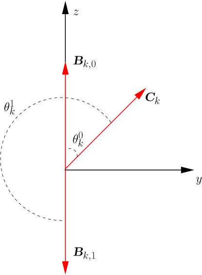
Figure 1: Bogoliubov rotation for fermion pairs.

The fermion operators $b_{k}$ and $b_{\bar{k}}$ are the Bogoliubov operators, and $R_{x}$ is the Bogoliubov transformation for fermion pairs. By noting that

$$\cos\theta_{k}^{s}=(-1)^{s}\left(1+\tan^{2}\theta_{k}^{s}\right)^{-1/2},$$ (6hijquvas)

for each pair of momenta one gets

$$H_{\gamma,k}^{(\varrho)}=\bm{C}_{k}^{\dagger}h_{\mathrm{\gamma}}(k)\bm{C}_{k}=(-1)^{s}\varepsilon_{k}^{(\varrho)}(g)\,\bm{B}_{k,s}^{\dagger}\sigma^{z}\bm{B}_{k,s},\quad k\in\mathcal{C}_{\varrho},\quad s\in\{0,1\},$$ (6hijquvat)

where $\varepsilon_{k}^{(\varrho)}$ is the dispersion relation for fermion pairs

$$\quad\varepsilon_{k}^{(\varrho)}(g)=\mathop{\mathrm{sgn}}\nolimits\!\left[\cos\frac{2\pi(\alpha+k)}{N}-g\right]\sqrt{\left[\cos\frac{2\pi(\alpha+k)}{N}-g\right]^{2}+\gamma^{2}\sin^{2}\frac{2\pi(\alpha+k)}{N}}.$$ (6hijquvau)

Here $\mathop{\mathrm{sgn}}\nolimits$ is the sign function, $\mathop{\mathrm{sgn}}\nolimits x=x/|x|$ for $x\neq 0$, and $\mathop{\mathrm{sgn}}\nolimits 0=0$. We stress that for each $k\in\mathcal{C}_{\varrho}$ the Bogoliubov rotation is defined independently on the other pairs, and so the sign of the dispersion relation can be chosen in a completely arbitrary way pair by pair. It is not difficult to show that the unitary operator on the Fock space $\mathcal{F}_{-}(\mathbb{C}^{N})$ corresponding to a Bogoliubov rotation $R_{x}(\theta)$,

$$b_{k}=U_{k}(\theta_{k}^{s})^{\dagger}\hat{c}_{k}U_{k}(\theta_{k}^{s}),\qquad b_{\bar{k}}=U_{k}(\theta_{k}^{s})^{\dagger}\hat{c}_{\bar{k}}U_{k}(\theta_{k}^{s}),$$ (6hijquvav)

reads

$$U_{k}(\theta)=\exp\left(-{\rm i}\frac{\theta}{2}K_{k}\right),\qquad K_{k}={\hat{c}}_{k}^{\dagger}\hat{c}_{\bar{k}}^{\dagger}+{\hat{c}}_{\bar{k}}\hat{c}_{k},\quad k\in\mathcal{C}_{\varrho}.$$ (6hijquvaw)

Its action on the Hamiltonian is

$$U_{k}(\theta_{k}^{s})H_{\gamma,k}^{(\varrho)}U_{k}(\theta_{k}^{s})^{\dagger}=(-1)^{s}\varepsilon_{k}^{(\varrho)}\left(\hat{c}_{k}^{\dagger}\hat{c}_{k}-\hat{c}_{\bar{k}}\hat{c}_{\bar{k}}^{\dagger}\right)\quad k\in\mathcal{C}_{\varrho}.$$ (6hijquvax)

Observe that since $K_{k}$ are quadratic with respect of creation and annihilation operators they commute with the parity operator (6hijn),

$$\mathcal{P}=U_{k}(\theta)\mathcal{P}U_{k}^{\dagger}(\theta),\quad k\in\mathcal{C}_{\varrho},$$ (6hijquvay)

and this means that the Bogoliubov transformation for fermion pairs preserves the parity sector. Finally, according to (6hijquvar) one gets the relation

$$U_{k}(\theta_{k}^{1})=V_{k\bar{k}}U_{k}(\theta_{k}^{0}),\quad\mathrm{with}\;V_{k\bar{k}}=U_{k}(\pi),\quad k\in\mathcal{C}_{\varrho}.$$ (6hijquvaz)

Note that the unitary operator $V_{k\bar{k}}$ can be decomposed in the form

$$V_{k\bar{k}}=S_{k\bar{k}}C_{k}C_{\bar{k}}$$ (6hijquvba)

where $C_{k}$ and $S_{k\bar{k}}$ are respectively the charge conjugation and the swapping operator

$$C_{k}\hat{c}_{k}C_{k}^{\dagger}=\hat{c}_{k}^{\dagger},$$ (6hijquvbba)

$$S_{k\bar{k}}\hat{c}_{k}S_{k\bar{k}}^{\dagger}=-{\rm i}\hat{c}_{\bar{k}},\quad k\in\mathcal{C}_{\varrho},$$ (6hijquvbbb)

whose explicit expressions are

$$C_{k}=\exp\left({\rm i}\frac{\pi}{2}(\hat{c}_{k}+\hat{c}_{k}^{\dagger})\right),$$ (6hijquvbbbca)

$$S_{k\bar{k}}=\exp\left({\rm i}\frac{\pi}{2}(\hat{c}_{k}^{\dagger}\hat{c}_{\bar{k}}+\hat{c}_{\bar{k}}^{\dagger}\hat{c}_{k})\right),\quad k\in\mathcal{C}_{\varrho}.$$ (6hijquvbbbcb)

Consider now the case of single fermions, $k\ \in\mathcal{S}_{\varrho}$. The set $\mathcal{S}_{\varrho}$ depends both on the parity sector and on the parity of $N$. For $N$ even one gets

$$\mathcal{S}_{\varrho}=\cases{\left\{[0],\left[\frac{N}{2}\right]\right\}&if $\varrho=-1$,\\ \emptyset&if $\varrho=+1$,}$$ (6hijquvbbbcbda)

while, for $$N$$ odd,

$$\mathcal{S}_{\varrho}=\cases{\{[0]\}&if $\varrho=-1$,\\ \left\{\left[\frac{N-1}{2}\right]\right\}&if $\varrho=+1$.}$$ (6hijquvbbbcbdb)

One can look at single fermions as a degenerate case of Bogoliubov pairs. Indeed, Equation (6hijquvao) reduces to

$$\tan\theta_{k}=0,\qquad k\in\mathcal{S}_{\varrho},$$ (6hijquvbbbcbdbe)

whose solutions are given by $\theta_{k}^{s}=s\pi$, with $s\in\{0,1\}$. Therefore, in this case we are free to choose between two possible unitary transformation: the identity and the charge conjugation,

$$U_{k}=(C_{k})^{0}=1,\qquad\mathrm{or}\quad U_{k}=C_{k},\qquad k\in\mathcal{S}_{\varrho}.$$ (6hijquvbbbcbdbf)

Note that, if charge conjugation is chosen, parity is not preserved; rather the two parity sectors are swapped by the Bogoliubov transformation,

$$\mathcal{P}=-C_{k}\mathcal{P}C_{k}^{\dagger}.$$ (6hijquvbbbcbdbg)

Finally, note that for single fermions the dispersion relation (6hijquvau) reduces to

$$\varepsilon_{k}^{(\varrho)}(g)=\cos\left(2\pi\frac{\alpha+k}{N}\right)-g,\qquad k\in\mathcal{S_{\varrho}},$$ (6hijquvbbbcbdbh)

since

$$\sin\left(2\pi\frac{\alpha+k}{N}\right)=0,\qquad k\in\mathcal{S_{\varrho}}.$$ (6hijquvbbbcbdbi)

In conclusion, the total Bogoliubov transformation that diagonalizes the Hamiltonian (6hijquvag) has the form

$$U_{B}(g,\gamma;\varrho,\bm{s})=\prod_{k\in\mathcal{C}_{\varrho}/\mathbb{Z}_{2}}U_{k}(\theta_{k})(V_{k\bar{k}})^{s_{k}}\prod_{j\in\mathcal{S}_{\varrho}}(C_{j})^{s_{j}},$$ (6hijquvbbbcbdbj)

where

$$\bm{s}=(s_{k})\in\{0,1\}^{N},\qquad\mathrm{with}\;s_{k}=s_{\bar{k}},$$ (6hijquvbbbcbdbk)

and $\mathcal{C}_{\varrho}/\mathbb{Z}_{2}$ denotes that, in the case of coupled fermions, one must consider only one element for each pair (orbit of $\mathbb{Z}_{2}$). Due to the constraint in (6hijquvbbbcbdbk), the Bogoliubov unitary transformation has a gauge freedom represented by the arbitrary choice of a binary vector of length $|\mathcal{S}_{\varrho}|+|\mathcal{C}_{\varrho}|/2$.

Note that the anti-commutation relations are preserved by the Bogoliubov transformation, while the parity sectors are swapped according to

$$\mathcal{P}=(-1)^{|\bm{s}|_{\varrho}}U_{B}(g,\gamma;\varrho,\bm{s})\,\mathcal{P}\,U_{B}(g,\gamma;\varrho,\bm{s})^{\dagger},$$ (6hijquvbbbcbdbl)

where

$$|\bm{s}|_{\varrho}=|\bm{s}_{\mathcal{S}_{\varrho}}|=\sum_{k\in\mathcal{S}_{\varrho}}s_{k}.$$ (6hijquvbbbcbdbm)

Therefore, one obtains the final expression of the diagonalized Hamiltonian

$$\tilde{H}_{\gamma}^{(\varrho)}(g) = U_{B}(g,\gamma;\varrho,\bm{s})H_{\gamma}^{(\varrho)}(g)U_{B}(g,\gamma;\varrho,\bm{s})^{\dagger}$$ (6hijquvbbbcbdbn)

$$= 2J\sum_{k\in\mathbb{Z}_{N}}(-1)^{s_{k}}\varepsilon_{k}^{(\varrho)}(g)\left(\hat{c}_{k}^{\dagger}\hat{c}_{k}-\frac{1}{2}\right)P_{\bar{\varrho}},$$

where

$$\bar{\varrho}=(-1)^{|\bm{s}|_{\varrho}}\varrho,$$ (6hijquvbbbcbdbo)

which depends on an arbitrary vector $\tilde{\bm{s}}\in\{0,1\}^{|\mathcal{S}_{\varrho}|+|\mathcal{C}_{\varrho}|/2}$, that generates $\bm{s}$ by the relation $s_{k}=s_{\bar{k}}=\tilde{s}_{k}$. Note that the physical part of $\tilde{H}_{\gamma}^{(\varrho)}$ acts on the sector of parity $\bar{\varrho}$.

2.3 XY ground state: vacua competition

One can use the gauge freedom of the Bogoliubov transformation (6hijquvbbbcbdbj) in the following convenient way. Let $\bm{s}=\bm{s}(g)$ be a function of the intensity of the magnetic field $g$, such that $(-1)^{s_{k}(g)}\,\varepsilon_{k}^{(\varrho)}(g)\geq 0$ for every $g\in\mathbb{R}$. From (6hijquvau) this means that

$$(-1)^{s_{k}(g)}=\mathop{\mathrm{sgn}}\nolimits\!\left[\cos\frac{2\pi(\alpha+k)}{N}-g\right],$$ (6hijquvbbbcbdbp)

that is

$$s_{k}(g)=\frac{1}{2}-\frac{1}{2}\mathop{\mathrm{sgn}}\nolimits\!\left[\cos\frac{2\pi(\alpha+k)}{N}-g\right].$$ (6hijquvbbbcbdbq)

Note that since $s_{\bar{k}}(g)=s_{k}(g)$, the above solution is consistent with the constraint (6hijquvbbbcbdbk) of $\bm{s}$. Therefore, the diagonalized expression of the XY Hamiltonian reads

$$H_{\gamma}^{(\varrho)}(g)=2J\sum_{k\in\mathbb{Z}_{N}}|\varepsilon_{k}^{(\varrho)}(g)|\left(\hat{c}_{k}^{\dagger}\hat{c}_{k}-\frac{1}{2}\right)P_{\bar{\varrho}(g)},\qquad\bar{\varrho}(g)=(-1)^{|\bm{s}(g)|_{\varrho}}\varrho.$$ (6hijquvbbbcbdbr)

With this choice one has that in each parity sector the lowest energy state is the one with zero fermions (vacuum state) whose energy density$\;/J$ is given by

$$E_{\rm vac}^{(-)}=-\frac{1}{N}\sum_{k\in\mathbb{Z}_{N}}\sqrt{\left[g-\cos\left(\frac{2\pi k}{N}\right)\right]^{2}+\gamma^{2}\sin^{2}\left(\frac{2\pi k}{N}\right)},$$ (6hijquvbbbcbdbsa)

$$E_{\rm vac}^{(+)}=-\frac{1}{N}\sum_{k\in\mathbb{Z}_{N}}\sqrt{\left[g-\cos\left(\frac{2\pi k}{N}+\frac{\pi}{N}\right)\right]^{2}+\gamma^{2}\sin^{2}\left(\frac{2\pi k}{N}+\frac{\pi}{N}\right)}.$$ (6hijquvbbbcbdbsb)

Note, however, that a condition must be satisfied: the Bogoliubov vacuum state is a physical state, provided that it has the right parity $\bar{\varrho}(g)$. Were this not the case, the projection $P_{\bar{\varrho}(g)}$ would automatically rule it out.

Let us look at the function $\bar{\varrho}(g)$ more closely. For $N$ even we have from (6hijquvbbbcbda) and (6hijquvbbbcbdbq)

$$|\bm{s}(g)|_{\varrho} = \left(s_{[0]}(g)+s_{\left[\frac{N}{2}\right]}(g)\right)\delta_{\varrho,-1}$$ (6hijquvbbbcbdbsbt)

$$= \left(1+\frac{1}{2}\mathop{\mathrm{sgn}}\nolimits(1-g)-\frac{1}{2}\mathop{\mathrm{sgn}}\nolimits(1+g)\right)\delta_{\varrho,-1},$$

whence

$$\bar{\varrho}(g)=(-1)^{|\bm{s}|_{\varrho}}\varrho=\delta_{\varrho,-1}\mathop{\mathrm{sgn}}\nolimits(1-g^{2})+\delta_{\varrho,+1},$$ (6hijquvbbbcbdbsbu)

that is

$$\bar{\varrho}(g)=\mathop{\mathrm{sgn}}\nolimits\!\left(1-\frac{1-\varrho}{2}g^{2}\right)\qquad(N\;\mathrm{even}).$$ (6hijquvbbbcbdbsbv)

For $N$ odd we have from (6hijquvbbbcbdb) and (6hijquvbbbcbdbq)

$$|\bm{s}(g)|_{\varrho} = s_{[0]}(g)\delta_{\varrho,-1}+s_{\left[\frac{N-1}{2}\right]}(g)\delta_{\varrho,+1}$$ (6hijquvbbbcbdbsbw)

$$= \frac{1}{2}-\frac{1}{2}\mathop{\mathrm{sgn}}\nolimits(1-g)\;\delta_{\varrho,-1}+\frac{1}{2}\mathop{\mathrm{sgn}}\nolimits(1+g)\;\delta_{\varrho,+1},$$

whence

$$\bar{\varrho}(g)=-\mathop{\mathrm{sgn}}\nolimits(1+\varrho g)\qquad(N\;\mathrm{odd}).$$ (6hijquvbbbcbdbsbx)

Since the vacuum state has $N$ holes, its parity is $(-1)^{N}$, and it is a physical state only if

$$\bar{\varrho}(g)=(-1)^{N}.$$ (6hijquvbbbcbdbsby)

Equation (6hijquvbbbcbdbsby) is satisfied for arbitrary $\varrho$ when $g\in(-1,1)$, while it is true only for $\varrho=(-1)^{N}$ for $g<-1$, and $\varrho=+1$ for $g>1$.

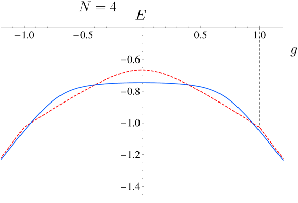
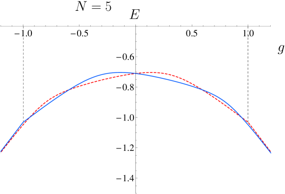
Figure 2: Vacua competition for $N=4$ and $5$ spins: for both cases the dashed line corresponds to $E_{\rm vac}^{(-)}$ and the solid one to $E_{\rm vac}^{(+)}$.

Therefore, for $g\in(-1,1)$, in the various regions of magnetic field $g$ the ground state is alternatively given by one of the two vacua with energy (6hijquvbbbcbdbsa)-(6hijquvbbbcbdbsb). We call this mechanism vacua competition between the two parity sectors. See Fig. 2.

For $g<-1$ the vacuum state with $\varrho=-1$ for $N$ even ($\varrho=+1$ for $N$ odd) is not physical, because it has the wrong parity $\bar{\varrho}=\varrho=-(-1)^{N}$, and it is ruled out from the competition by the projection $P_{\bar{\varrho}}$. Analogously, for $g>1$ the vacuum state with $\varrho=-1$ for both $N$ even and odd is ruled out. However, it is not difficult to prove that the energy of the unphysical vacuum when $|g|>1$ is always larger than the physical one. Therefore, as far as one is interested in the ground state, the ground state is the result of the vacua competition in the whole range $g\in\mathbb{R}$. Not so for the first excited level, which is the energy of the “losing” vacuum only in the range $(-1,1)$, while outside it is the lowest 1-fermion energy level above the losing vacuum.

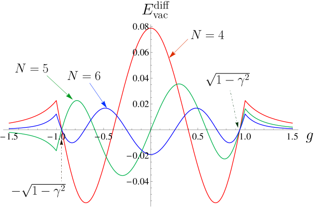
Figure 3: Difference between energy densities (in unit $J$) of the two vacua at $\gamma=\frac{1}{3}$ for even numbers of spins, $N=4,5,6$. For all $N$, $E_{\rm vac}^{\rm diff}$ vanishes at $g=\sqrt{1-\gamma^{2}}$.

More generally, from (6hijquvbbbcbdbsbv) and (6hijquvbbbcbdbsbx) it easily follows that the whole spectrum is given for $g\in(-1,1)$ by the union of the spectra of eigenstates with an even number of Bogoliubov fermions ($\bar{\varrho}=(-1)^{N}$) of both Hamiltonians $\tilde{H}_{\gamma}^{(\varrho)}$ with $\varrho=\pm 1$. On the other hand, outside the above interval, the spectrum is given by the eigenstates of $\tilde{H}_{\gamma}^{(\varrho)}$ ($\tilde{H}_{\gamma}^{(-\varrho)}$) with an even (odd) number of Bogoliubov particles, where $\varrho=(-1)^{N}$ for $g<-1$ and $\varrho=+1$ for $g>1$. The intersection points between the vacua energy densities depend in general on the number of spins $N$; however, independently of $N$, the difference between the two energy densities,

$$E_{\rm vac}^{\rm diff}(g)=E_{\rm vac}^{(-)}-E_{\rm vac}^{(+)}=-\frac{1}{N}\sum_{m\in\mathbb{Z}_{2N}}(-1)^{m}\sqrt{\left[g-\cos\left(\frac{\pi m}{N}\right)\right]^{2}+\gamma^{2}\sin^{2}\left(\frac{\pi m}{N}\right)},$$ (6hijquvbbbcbdbsbz)

always vanishes at $g=\pm\sqrt{1-\gamma^{2}}$ (see figure 3). Indeed one has

$$E_{\rm vac}^{\rm diff}(\pm\sqrt{1-\gamma^{2}}) = -\frac{1}{N}\sum_{k\in\mathbb{Z}_{2N}}(-1)^{m}\left[1\mp\sqrt{1-\gamma^{2}}\cos\left(\frac{\pi m}{N}\right)\right]$$ (6hijquvbbbcbdbsca)

and

$$\sum_{k\in\mathbb{Z}_{2N}}(-1)^{m}\cos\left(\frac{\pi m}{N}\right)={\rm Re}\left(\frac{1-\mathrm{e}^{\mathrm{i}2\pi(N+1)}}{1-\mathrm{e}^{\mathrm{i}\pi(N+1)/N}}\right)=0.$$ (6hijquvbbbcbdbscb)

From figure 3 on can also observe that for finite size systems the vacua intersection points present discontinuities of the first derivative, as will be explicitly shown in section 4. In that section we will also focus on the points $g=\pm 1$ which are two interesting values of the magnetic field for this class of Hamiltonians, since they will be shown to represent the finite-size forerunners of the quantum phase transition points (in the thermodynamic limit).

3 The XX model

The XX model ($\gamma=0$) is known as the isotropic model since the interaction between nearest neighbours spins along $x$ and $y$ axis is characterized by the same coefficient in the Hamiltonian (1):

$$H_{XX}(g)=H_{\gamma=0}(g)=-J\sum_{i\in\mathbb{Z}_{N}}\Big{[}g\sigma_{i}^{z}+\frac{1}{2}\sigma_{i}^{x}\sigma_{i+1}^{x}+\frac{1}{2}\sigma_{i}^{y}\sigma_{i+1}^{y}\Big{]}.$$ (6hijquvbbbcbdbscc)

In this case equation (6hijquvab) reduces to

$$\qquad H_{0}^{(\varrho)}(g)=2J\sum_{k\in\mathbb{Z}_{N}}\left[\cos\left(2\pi\frac{\alpha+k}{N}\right)-g\right]\left(\hat{c}_{k}\hat{c}_{k}^{\dagger}-\frac{1}{2}\right)P_{\varrho},\qquad\alpha=\frac{1+\varrho}{4}.$$ (6hijquvbbbcbdbscd)

From this follows that the Fourier transformed XX Hamiltonian is already diagonal and the last term characterizing coupled fermions in Equation (6hijquvab) vanishes for all $k$. In other words in the XX model we are only dealing with single fermions, $\mathcal{S}_{\varrho}=\mathbb{Z}_{N}$, and the Bogoliubov transformation (6hijquvbbbcbdbj) reduces to

$$U_{B}(g;\varrho,\bm{s})=\prod_{k\in\mathbb{Z}_{N}}C_{k}^{s_{k}},$$ (6hijquvbbbcbdbsce)

where now $\bm{s}\in\{0,1\}^{N}$ is an unconstrained binary string of length $N$. This yields

$$\tilde{H}_{0}^{(\varrho)}(g) = U_{B}(g;\varrho,\bm{s})H_{0}^{(\varrho)}(g)U_{B}(g;\varrho,\bm{s})^{\dagger}$$ (6hijquvbbbcbdbscf)

$$= 2J\sum_{k\in\mathbb{Z}_{N}}(-1)^{s_{k}}\left[\cos\left(2\pi\frac{\alpha+k}{N}\right)-g\right]\left(\hat{c}_{k}\hat{c}_{k}^{\dagger}-\frac{1}{2}\right)P_{\bar{\varrho}}$$

with $\bar{\varrho}=(-1)^{|\bm{s}|}\varrho$. In particular, if $s_{k}=0$ the Bogoliubov transformation associates JW fermions to Bogoliubov fermions, while if $s_{k}=1$ it transforms JW fermions into Bogoliubov antifermions, or holes.

3.1 The energy spectrum

As already emphasized at the end of section 2.2, the energy spectrum does not depend on the choice of the gauge $\bm{s}$ of the unitary Bogoliubov transformation. If $\bm{s}=0$ equation (6hijquvbbbcbdbscf) becomes

$$\tilde{H}_{0}^{(\varrho)}=H_{0}^{(\varrho)}=2J\sum_{k\in\mathbb{Z}_{N}}\left[\cos\left(2\pi\frac{\alpha+k}{N}\right)-g\right]\left(\hat{c}_{k}^{\dagger}\hat{c}_{k}-\frac{1}{2}\right)P_{\varrho},$$ (6hijquvbbbcbdbscg)

The spectrum of the above Hamiltonian, and in particular its ground state energy has been studied in [22]. We quickly summarize the main results and show how they derive from vacua competition. The energy density$/J$ of the vacuum state does not depend on the parity $\varrho$ and on the size $N$

$$E_{\rm{vac}}(g)=\frac{1}{N}\sum_{k\in\mathbb{Z}_{N}}\left[g-\cos\!\left(2\pi\frac{\alpha+k}{N}\right)\right]=g.$$ (6hijquvbbbcbdbsch)

On the other hand, if we add one fermion of momentum $k$ the energy density reads

$$E_{1}^{(\varrho)}(k,g)=E_{\rm{vac}}(g)-\frac{2}{N}\left[g-\cos\!\left(2\pi\frac{\alpha+k}{N}\right)\right],\qquad\alpha=\frac{1+\varrho}{2}$$ (6hijquvbbbcbdbsci)

where $\varrho=-(-1)^{N}$ is the parity of the 1-particle sector. In figure 4 we represent the single particle energy spectra corresponding to $N=8$ and $9$ sites (representative of an even/odd number of spins, respectively). The different lines are parametrized by $k\in\mathbb{Z}_{N}$ and one notes the presence of degeneracies in both cases. Since we are interested in the ground state of the system, we focus on the lowest energy levels and consider the values assumed by the function $\cos[2\pi(\alpha+k)/N]$ in the four possible cases ($N$ even or odd and $\alpha\equiv 0$ or $1/2\mathop{\mathrm{mod}}\nolimits N$), as shown in Fig. 5. Notice that these results can be described in terms of regular polygons inscribed in a circle of unit radius, see figure 6.

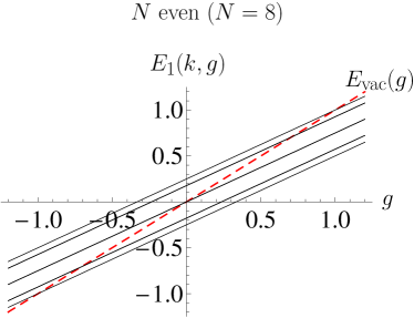
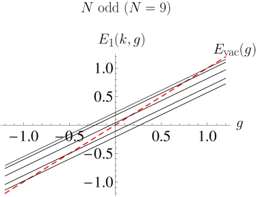
Figure 4: Single particle energy densities $E_{1}(k,g)$ (solid lines) and vacuum energy densities $E_{\rm vac}(g)$ (dashed lines). Different lines correspond to different $k\in\mathbb{Z}_{N}$ according to (6hijquvbbbcbdbsci).

Figure 5: Plot of $\cos[2\pi(\alpha+k)/N]$, $k\in\mathbb{Z}_{N}$ for $N=8,9$ and $\alpha\equiv 0,1/2\;(\mathop{\mathrm{mod}}\nolimits N)$.

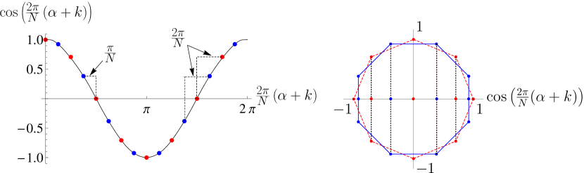
Figure 6: (Color online) Left: plot of $\cos[2\pi(\alpha+k)/N]$, $k\in\mathbb{Z}_{N}$ with $\alpha\equiv 0\;(\mathop{\mathrm{mod}}\nolimits N)$ (dashed line) and $\alpha=1/2\;(\mathop{\mathrm{mod}}\nolimits N)$ (solid line), for $N=8$. Right: geometrical description of $\cos[2\pi(\alpha+k)/N]$ for $N=8$.

From figure 5 one obtains the values of $k$ that minimize the energy per site; in the 1-particle sector one has

$$\left\{\begin{array}[]{l@{\quad}l@{\quad}l@{}l}\vskip 6.0pt plus 2.0pt minus 2.0ptN\ {\rm even}&\Rightarrow&\alpha\equiv 0&\ {\rm mod}\ N\Rightarrow k=\left[\frac{N}{2}\right],\\ N\;{\rm odd}&\Rightarrow&\alpha\equiv\frac{1}{2}&\ {\rm mod}\ N\Rightarrow k=\left[\frac{N-1}{2}\right].\end{array}\right.$$ (6hijquvbbbcbdbscj)

Similarly, in the 2-particle sector the energy is minimum for

$$\left\{\begin{array}[]{l@{\quad}l@{\quad}l@{}l}\vskip 6.0pt plus 2.0pt minus 2.0ptN\;\mbox{even}&\Rightarrow&\alpha\equiv\frac{1}{2}&\ {\rm mod}\ N\Rightarrow\{k_{1},k_{2}\}=\left\{\left[\frac{N}{2}-1\right],\left[\frac{N}{2}\right]\right\},\\ N\;\mbox{odd}&\Rightarrow&\alpha\equiv 0&\ {\rm mod}\ N\Rightarrow\{k_{1},k_{2}\}=\left\{\left[\frac{N-1}{2}\right],\left[\frac{N+1}{2}\right]\right\}.\end{array}\right.$$ (6hijquvbbbcbdbsck)

It turns out that the general expression of the lowest energy levels in the different $n$-particle sectors does not depend on the parity of $N$. For $n$ fermions, one gets [22]

$$E_{n}^{\rm min}(g)=g\left(1-\frac{2n}{N}\right)-\frac{2}{N}\frac{\sin(n\pi/N)}{\sin(\pi/N)}.$$ (6hijquvbbbcbdbscl)

In figure 7 we plot the lowest energy levels corresponding to $0\leq n\leq N$ for $N=8$ sites. The intersections of levels corresponding to $n$ and $n+1$ fermions (starting from $n=0$) define the points of level crossing $g_{c}$, where an excited level and the ground state are interchanged. The analytic expression of the critical points is easily obtained by the condition $E_{n}^{\rm min}(g_{c})=E_{n+1}^{\rm min}(g_{c})$. We find

$$g_{c}(n) = (-1)^{n+1}\left[1+2\sum_{m=1}^{n}\cos\left(\frac{\pi m}{N}\right)\right]$$ (6hijquvbbbcbdbscm)

$$= \frac{\sin(n\pi/N)-\sin[(n+1)\pi/N]}{\sin(\pi/N)},\qquad 0\leq n\leq N-1.$$ (6hijquvbbbcbdbscn)

As a consequence, the ground-state energy density is

$$\qquad E_{\rm gs}(g)=g\left(1-\frac{2n}{N}\right)-\frac{2}{N}\frac{\sin(n\pi/N)}{\sin(\pi/N)}\quad{\rm with}\quad g\in\Big{(}g_{c}(n-1),g_{c}(n)\Big{)},$$ (6hijquvbbbcbdbsco)

with $0\leq n\leq N$ and where we stipulated that $g_{c}(-1)=-\infty$ and $g_{c}(N)=+\infty$. Thus, for $g\in(g_{c}(n-1),g_{c}(n))$, the ground state contains $n$ JW fermions. Note that $g_{c}(0)=-1$ and $g_{c}(N-1)=+1$, independently of $N$.

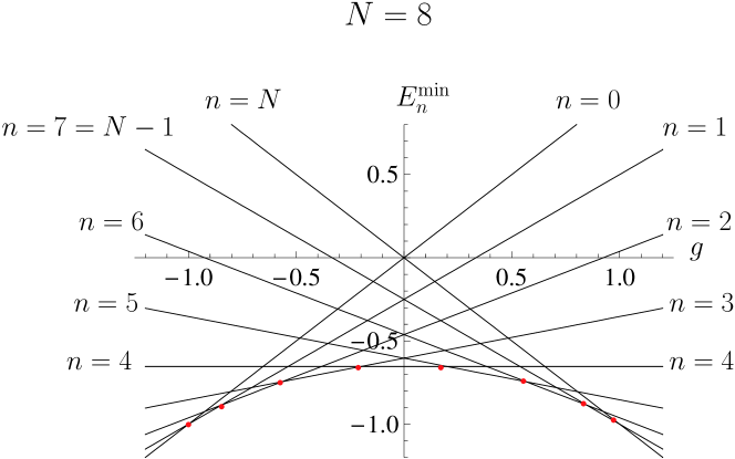
Figure 7: Lowest energy levels $E_{n}^{\rm min}(g)$ for different number of fermions $n$; the intersection between the energy levels corresponding to $n$ and $n+1$ fermions (starting from $n=0$) are the points of level crossing (dots).

We will now derive the ground state energy density starting from the same choice of the Bogoliubov transform made for the XY Model (6hijquvbbbcbdbr) that particularizes to

$$\tilde{H}^{(\varrho)}_{0}(g)=2J\sum_{k\in\mathbb{Z}_{N}}\left|\cos\left(2\pi\frac{\alpha+k}{N}\right)-g\right|\left(\hat{c}_{k}^{\dagger}\hat{c}_{k}-\frac{1}{2}\right)P_{\bar{\varrho}(g)},$$ (6hijquvbbbcbdbscp)

$$\bar{\varrho}(g)=(-1)^{|\bm{s}(g)|}\varrho.$$ (6hijquvbbbcbdbscq)

The ground state is then the winner of the vacua competition between

$$E_{\rm vac}^{(-)}(g)=-\frac{1}{N}\sum_{k\in\mathbb{Z}_{N}}\left|\cos\left(\frac{2\pi k}{N}\right)-g\right|,$$ (6hijquvbbbcbdbscra)

$$E_{\rm vac}^{(+)}(g)=-\frac{1}{N}\sum_{k\in\mathbb{Z}_{N}}\left|\cos\left(\frac{2\pi k}{N}+\frac{\pi}{N}\right)-g\right|$$ (6hijquvbbbcbdbscrb)

(see Fig. 8).

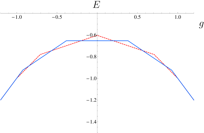
Figure 8: The ground state energy density of the XX model ($N=8$) is given by the competition between the vacua energy densities $E_{\rm vac}^{(-)}$ (dashed line) and $E_{\rm vac}^{(+)}$ (solid line).

The points of level crossing (6hijquvbbbcbdbscm) are given by those values of the magnetic field that satisfy the following equation

$$E^{\rm diff}_{\rm vac}(g)=-\frac{1}{N}\sum_{k\in\mathbb{Z}_{2N}}(-1)^{k}\left|\cos\left(\frac{\pi k}{N}\right)-g\right|=0.$$ (6hijquvbbbcbdbscrcs)

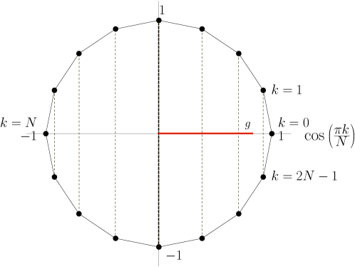
Figure 9: Geometrical representation of Equation (6hijquvbbbcbdbscrcs) when $N=8$; the thick red line is the magnetic field $g$.

Consider the regular polygon inscribed in a circle of unit radius in figure 9; it is a geometrical representation of the function $\cos\left(\frac{\pi k}{N}\right)$ for $k\in\mathbb{Z}_{N}$. When $|g|>1$ one immediately gets $E^{\rm diff}_{\rm vac}(g)=0$, whereas for $|g|\leq 1$ the key idea is to consider the $N$ intervals on the $x$ axis limited by the dashed vertical lines, represented in figure 9; for each interval one can write the explicit expression for the vacua difference (6hijquvbbbcbdbscrcs). For example when $g\in\left[\cos\left(\frac{\pi}{N}\right),1\right]$ one gets

$$E^{\rm diff}_{\rm vac}(g) = -\frac{1}{N}\left[(1-g)+\sum_{k\in\mathbb{Z}_{2N},k\neq[0]}(-1)^{k}\left(g-\cos\left(\frac{\pi k}{N}\right)\right)\right]$$ (6hijquvbbbcbdbscrct)

$$= -\frac{1}{N}\left[2(1-g)+\sum_{k\in\mathbb{Z}_{2N}}(-1)^{k}\left(g-\cos\left(\frac{\pi k}{N}\right)\right)\right]$$

$$= -\frac{2}{N}(1-g),$$

from which follows that in this interval $E^{\rm diff}_{\rm vac}(g)=0$ for $g=1$. Similarly when $g\in\left[\cos\frac{(m+1)\pi}{N},\cos\frac{m\pi}{N}\right]$, for $0\leq m\leq N-1$, one gets that $E^{\rm diff}_{\rm vac}(g)=0$ when

$$g=(-1)^{m}\left(1+2\sum_{k=1}^{m}\cos\left(\frac{\pi k}{N}\right)\right)=-g_{c}(m),\qquad 0\leq m\leq N-1,$$ (6hijquvbbbcbdbscrcu)

where $g_{c}(m)$ are the points of level crossing (6hijquvbbbcbdbscm) [for $n=0$ one gets $g=1$, in agreement with (6hijquvbbbcbdbscrcs)]. By considering the symmetry $g_{c}(n)=-g_{c}(N-1-n)$, one immediately sees that the level crossing points have the same analytic expression of the intersection points between the two vacua, for $n=N-1-m$.

4 Thermodynamic limit and quantum phase transitions

4.1 Quantum phase transitions in the XY model

In this section we will show that in finite size systems one can find the forerunners of the points of quantum phase transition. These points are characterized by the presence of large values of the second derivative of the ground state energy density, that is then amplified and becomes a singularity in the thermodynamic limit.

As observed in section 2.3, the first derivative of the ground state energy evaluated at the intersection points between the two vacua is not continuous and for finite size systems the second derivatives diverges at these points; however we will show that these singularities vanish when $N\rightarrow\infty$. Consider for example the level crossing at $g=\sqrt{1-\gamma^{2}}$; the difference between the first derivatives of the two vacuum energies is given by the derivative of (6hijquvbbbcbdbsbz):

$$\frac{{\rm d}E_{\rm vac}^{\rm diff}}{{\rm d}g}(\sqrt{1-\gamma^{2}}) = \frac{1}{N}\frac{\gamma^{2}}{\sqrt{1-\gamma^{2}}}\sum_{k\in\mathbb{Z}_{N}}\Bigg{[}\frac{1}{1-\sqrt{1-\gamma^{2}}\cos\left({\frac{2\pi k}{N}+\frac{\pi}{N}}\right)}$$ (6hijquvbbbcbdbscrcv)

$$\phantom{\frac{1}{N}\frac{\gamma^{2}}{\sqrt{1-\gamma^{2}}}\sum_{k\in\mathbb{Z}_{N}}\Bigg{[}}-\frac{1}{1-\sqrt{1-\gamma^{2}}\cos\left({\frac{2\pi k}{N}}\right)}\Bigg{]}.$$

When the number of spins $N$ is odd, for each $k\in\mathbb{Z}_{N}$ there is a given $\tilde{k}=k+\frac{N}{2}$ such that $\cos\left(\frac{2\pi k}{N}\right)=-\cos\left(\frac{2\pi\tilde{k}}{N}+\frac{\pi}{N}\right)$ (see Fig.  10), and the last equation becomes

$$\;\;\frac{{\rm d}E_{\rm vac}^{\rm diff}}{{\rm d}g}\left(\sqrt{1-\gamma^{2}}\right)=\frac{1}{N}\frac{\gamma^{2}}{\sqrt{1-\gamma^{2}}}\left[\frac{2\sqrt{1-\gamma^{2}}}{\gamma^{2}}+4\sum_{k=1}^{(N-1)/2}\frac{\cos\left(\frac{2\pi k}{N}\right)\sqrt{1-\gamma^{2}}}{1-\cos\left(\frac{2\pi k}{N}\right)(1-\gamma^{2})}\right];$$ (6hijquvbbbcbdbscrcw)

from the symmetries of the function $\cos\left(\frac{2\pi k}{N}\right)$ one gets that the last expression is strictly greater than zero. From this it follows that the second derivative of the vacua energy difference diverges for all finite $N$ at $g=\sqrt{1-\gamma^{2}}$, and the same argument can be extended to all intersection points between the two vacua.

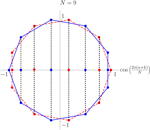
Figure 10: Geometrical description for $\cos\left(\frac{2\pi(\alpha+k)}{N}\right)$ for $N=9$, similar to figure 6: the two polygons belong to the parity sectors $\alpha=0\;(\mathop{\mathrm{mod}}\nolimits N)$ (dashed line) and $\alpha\equiv 1/2\;(\mathop{\mathrm{mod}}\nolimits N)$ (solid line)

The case $N$ even, see figure 6, is analogous, as one can see by noting that the polygon corresponding to $\alpha\equiv\frac{1}{2}(\mathop{\mathrm{mod}}\nolimits N)$ is rotated by an angle $\frac{\pi}{N}$ (or in other words, it associates to each momentum $k\mapsto\tilde{k}=k+\frac{N-1}{2}$).

Summarizing, for finite size systems the second derivative of the energy density of the ground state diverges at the intersection points of the two vacua; on the other hand in the thermodynamic limit this divergence is suppressed. Indeed, in the limit $N\to\infty$ equation (6hijquvbbbcbdbscrcv) becomes:

$$\frac{{\rm d}E_{\rm vac}^{\rm diff}}{{\rm d}g}\left(\sqrt{1-\gamma^{2}}\right)\sim\frac{\gamma^{2}}{2\pi\sqrt{1-\gamma^{2}}}\int_{0}^{2\pi}{\rm d}x\left(f(x)-f(x+\pi/N)\right),$$ (6hijquvbbbcbdbscrcx)

where $f(x)$ is given by:

$$f(x)=\frac{1}{1-\sqrt{1-\gamma^{2}}\cos(x)}.$$ (6hijquvbbbcbdbscrcy)

Expanding in Taylor series $f(x+\pi/N)$ one gets

$$\frac{{\rm d}E_{\rm vac}^{\rm diff}}{{\rm d}g}\left(\sqrt{1-\gamma^{2}}\right)\to\frac{\gamma^{2}}{\pi\sqrt{1-\gamma^{2}}}f^{\prime}(0)=0,\qquad N\to\infty.$$ (6hijquvbbbcbdbscrcz)

This means that the singularities of the second derivative of the ground state vanish in the thermodynamic limit; in other words, the forerunners of the quantum phase transition are not related to finite-size level crossings of the ground state. In this section we will show that they are related to the level crossings between the unphysical vacuum and the losing physical vacuum where single Bogoliubov fermions sit.

Consider the explicit expressions of the vacua energies corresponding to the four possible cases given by the parity of $N$ and the two parity sectors

1. $N$ even, $\varrho=-1$, $\mathcal{S}_{\varrho}=\left\{[0],\left[\frac{N}{2}\right]\right\}$,

   $$E_{\rm vac}^{(-)}=-\frac{1}{N}\Bigg{[}\sum_{k\in\mathcal{C}_{\varrho}}\sqrt{\left[g-\cos\left(\frac{2\pi k}{N}\right)\right]^{2}+\gamma^{2}\sin^{2}\left(\frac{2\pi k}{N}\right)}+|g-1|+|g+1|\Bigg{]};$$ (6hijquvbbbcbdbscrdaa)

2. $N$ odd, $\varrho=-1$, $\mathcal{S}_{\varrho}=\left\{[0]\right\}$,

   $$E_{\rm vac}^{(-)}=-\frac{1}{N}\Bigg{[}\sum_{k\in\mathcal{C}_{\varrho}}\sqrt{\left[g-\cos\left(\frac{2\pi k}{N}\right)\right]^{2}+\gamma^{2}\sin^{2}\left(\frac{2\pi k}{N}\right)}+|g-1|\Bigg{]};$$ (6hijquvbbbcbdbscrdab)

3. $N$ even, $\varrho=+1$, $\mathcal{S}_{\varrho}=\emptyset$,

   $$E_{\rm vac}^{(+)}=-\frac{1}{N}\sum_{k\in\mathbb{Z}_{N}}\sqrt{\left[g-\cos\left(\frac{2\pi k}{N}+\frac{\pi}{N}\right)\right]^{2}+\gamma^{2}\sin^{2}\left(\frac{2\pi k}{N}+\frac{\pi}{N}\right)};$$ (6hijquvbbbcbdbscrdac)

4. $N$ odd, $\varrho=+1$, $\mathcal{S}_{\varrho}=\left\{\left[\frac{N-1}{2}\right]\right\}$,

   $$E_{\rm vac}^{(+)}=-\frac{1}{N}\Bigg{[}\sum_{k\in\mathcal{C}_{\varrho}}\sqrt{\left[g-\cos\left(\frac{2\pi k}{N}+\frac{\pi}{N}\right)\right]^{2}+\gamma^{2}\sin^{2}\left(\frac{2\pi k}{N}+\frac{\pi}{N}\right)}+|g+1|\Bigg{]}.$$

   (6hijquvbbbcbdbscrdad)

Observe that the absolute values in the previous expressions correspond to the cosines evaluated at single fermion momenta $\mathcal{S}_{\varrho}$; at these values of the magnetic field the first derivative of energy is not continuous (see figure 2) and the second derivative has terms proportional to the Dirac delta functions $\delta(g\pm 1)$. However, remember that the vacuum in case (i) becomes unphysical as soon as $|g|>1$, so that at $g=\pm 1$ there is a level crossings between physical and unphysical states. The same phenomenon happens to the vacuum in case (ii) at $g=1$, and to the vacuum in case (iv) at $g=-1$. On the other hand, one can observe that for finite size chains, for both even and odd $N$, the ground state is smooth at $g=\pm 1$, in other words the ground state, which coincides with the winning vacuum state, does not have any singularities at these points. However, it can be shown that the second derivative of the ground state energy at $g=\pm 1$ scales as $-\log N$ .

Consider for example the case of an even number of spins $N$. In this case the ground state belongs to the parity sector with $\varrho=+1$, without singularities. Figure 11 displays ${\rm d}^{2}E_{\rm vac}^{(+)}/{\rm d}g^{2}$ for $N=6,24,54$; at $g=\pm 1$ it scales like $-\log N$.

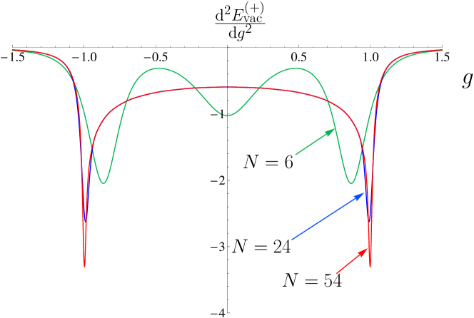
Figure 11: Second derivative of the vacuum energy density for even values of $N$, in the parity sector $\varrho=+1$.

Indeed when $g=1$, by deriving (6hijquvbbbcbdbsb) one has

$$\qquad\frac{{\rm d}^{2}E_{\rm vac}^{(+)}}{{\rm d}^{2}g}\left(1\right) = -\frac{\gamma^{2}}{N}\sum_{k\in\mathbb{Z}_{N}}\frac{\left(1+\cos\left(\frac{2\pi k}{N}+\frac{\pi}{N}\right)\right)^{3/2}}{\left|\sin\left(\frac{2\pi k}{N}+\frac{\pi}{N}\right)\right|\left[1+\gamma^{2}+\cos\left(\frac{2\pi k}{N}+\frac{\pi}{N}\right)(\gamma^{2}-1)\right]^{3/2}}$$ (6hijquvbbbcbdbscrdadb)

$$\simeq -\frac{1}{\gamma\pi}\left[3+\log\left(\frac{N}{8}-\frac{1}{2}\right)\right]-\frac{1}{2}\frac{\gamma^{2}}{\left(1+\gamma^{2}\right)^{3/2}}\sim-\frac{1}{\gamma\pi}\log N,$$

for $N\to\infty$, as shown in figure 12.

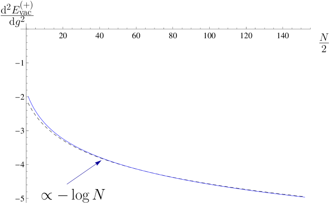
Figure 12: Second derivative of the vacuum energy density at $g=1$ in the parity sector $\varrho=+1$ for $N$ even, from $18$ to $320$ (dashed line): it scales as $-\log N$ (solid line).

The cases $g=-1$ and $N$ even ($\varrho=+1$) and $g=\pm 1$ and $N$ odd ($\varrho=\mp 1$) are analogous.

The quantum phase transition is forerun by the losing vacuum whose second derivative contains a Dirac delta function, at the transition between physical and unphysical states. When $N$ tends to infinity, as we will now show, the difference between the two vacua at $g=\pm 1$ tends to zero and quantum phase transition forerunners approach the ground state, building up singularities at logarithmic rates. Indeed, at $g=\pm 1$ from Equation (6hijquvbbbcbdbsbz) one has:

$$E_{\rm vac}^{\rm diff}(\pm 1)=+\frac{1}{N}\sum_{k\in\mathbb{Z}_{N}}f_{\pm}\left(\frac{2\pi k}{N}+\frac{\pi}{N}\right)-f_{\pm}\left(\frac{2\pi k}{N}\right),$$ (6hijquvbbbcbdbscrdadc)

where

$$f_{\pm}(x)=\sqrt{\left(\pm 1-\cos x\right)^{2}+\gamma^{2}\sin^{2}x}.$$ (6hijquvbbbcbdbscrdadd)

In the thermodynamic limit, by applying the same technique used in (6hijquvbbbcbdbscrcx), equation (6hijquvbbbcbdbscrdadc) becomes

$$E_{\rm vac}^{\rm diff}(\pm 1) \sim -\frac{1}{2\pi}\int_{0}^{2\pi}\left[f\left(x+\frac{\pi}{N}\right)-f(x)\right]\mathrm{d}x$$ (6hijquvbbbcbdbscrdade)

$$\sim -\frac{1}{2\pi}\frac{\pi^{2}}{2!N^{2}}\int_{0}^{2\pi}f^{\prime\prime}(x){\rm d}x\sim\frac{\pi}{2N^{2}}\gamma,\qquad N\to\infty,$$

where we used the equality $f^{\prime}_{\pm}(0)=-\gamma$. See figure 13.

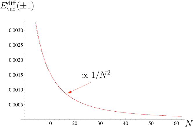
Figure 13: Difference between the two vacua energy densities at $g=\pm 1$: exact result (dotted line) and asymptotic approximation of order $1/N^{2}$ (solid line).

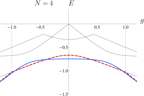
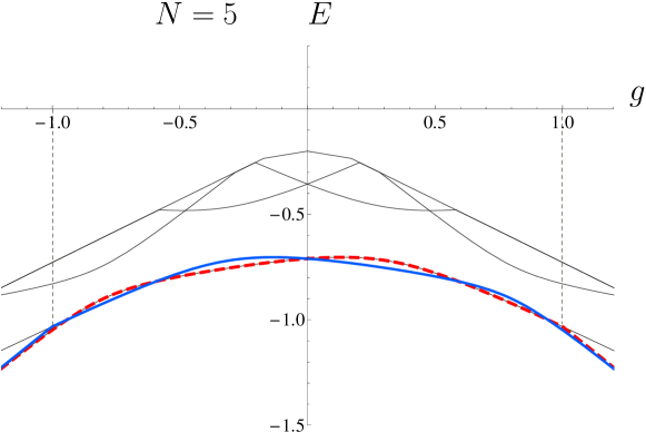
Figure 14: The thin lines represent the low energy part of the spectrum of the XY chain, and the thick solid and dashed lines refer to the two vacua energy densities, $E_{\rm vac}^{(-)}$ and $E_{\rm vac}^{(+)}$, respectively: these vacua alternatively coincide with the ground state and the first excited state for $|g|\leq 1$. When $g=\pm 1$ one vacuum energy is the ground state energy, while the other one does not corresponds to any physical level. The transition points are the forerunners of the quantum phase transition.

In figure 14 we display the low energy part of the spectrum (thin lines) and the energy density of the two vacua (thick lines): at $g=\pm 1$ the ground state is the winning vacuum that has no singularities, the first excited level coincide with the losing vacuum for $g\in(-1,1)$. Its second derivative diverges at $g=\pm 1$, forerunning the quantum phase transitions. Observe that they are at the transition between a physical state, which coincides with the first excited level, and an unphysical state, which does not corresponds to any physical level: for $|g|>1$ the losing vacuum is unphysical. Summarizing, we identify as forerunners of the quantum phase transition those points of the losing vacuum energy density whose second derivative diverges. These points are associated to single Bogoliubov fermions and belong to the crossing between the first excited level and the unphysical vacuum for finite size systems. When $N\rightarrow\infty$ they approach the ground state as $N^{-2}$.

4.2 Quantum phase transitions in the XX model

As observed in Section 3 the XX model ($\gamma=0$) is characterized by the only presence of single fermions, and the absence of Bogoliubov pairs. As a result, all points $g=\cos\left(\frac{2\pi(\alpha+k)}{N}\right)$ (in both parity sectors) with $k\in\mathbb{Z}_{N}$ can be considered quantum phase transitions forerunners.

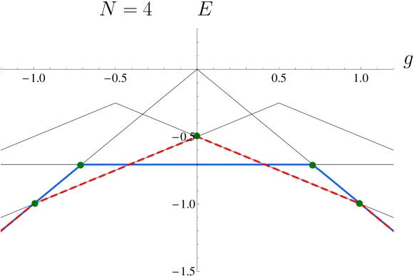
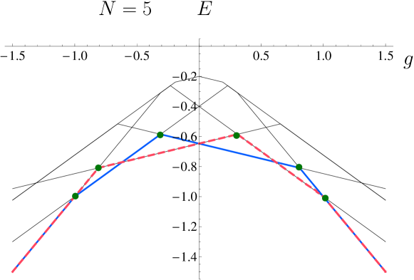
Figure 15: The thin lines represent the low energy part of the spectrum of the XX chain with $N=4$ and $N=5$ spins; the solid and dashed tick lines refer the two vacua energy densities in the parity sectors with $\varrho=-1$ and $\varrho=+1$, respectively. The forerunners of the (continuous) quantum phase transition points are indicated with bold points; they are given by $g_{k}=\cos\left(\frac{2\pi k}{N}\right)$, $k\in\mathbb{Z}_{N}$.

See (6hijquvbbbcbdbscra)-(6hijquvbbbcbdbscrb) and compare with (6hijquvbbbcbdbscrdaa)-(6hijquvbbbcbdbscrdad). Indeed, the second derivative of the vacua energy density contains a Dirac delta function at these points and, apart from $g=\pm 1$, they all belong to the first excited level like in the XY model, see Fig. 15 (we will focus on $g=\pm 1$ at the end of this section). In the thermodynamic limit these points forerunning the quantum phase transition approach the ground state, becoming critical points. Consider for example $g_{\ell}=\cos\left(\frac{2\pi\ell}{N}\right)\neq\pm 1$; the energy difference between the vacua is now given by

$$E_{\rm vac}^{\rm diff}(g_{\ell})\! = \!-\frac{1}{N}\!\sum_{k\in\mathbb{Z}_{N}\backslash\{\ell\}}\!\!\left[\left|\cos\left(\frac{2\pi\ell}{N}\right)-\cos\left(\frac{2\pi k}{N}\right)\right|-\left|\cos\left(\frac{2\pi\ell}{N}\right)-\cos\left(\frac{2\pi k}{N}+\frac{\pi}{N}\right)\right|\right]$$ (6hijquvbbbcbdbscrdadf)

$$+\frac{1}{N}\left|\cos\left(\frac{2\pi\ell}{N}\right)-\cos\left(\frac{2\pi\ell}{N}+\frac{\pi}{N}\right)\right|.$$

By using the same technique of the previous section one gets

$$\qquad E_{\rm vac}^{\rm diff}(g_{\ell}) = \frac{1}{2\pi}\int_{0}^{2\pi}\left[\frac{\pi}{N}f^{\prime}_{\ell}(x)+\left(\frac{\pi}{N}\right)^{2}\frac{f^{\prime\prime}_{\ell}(x)}{2!}+\left(\frac{\pi}{N}\right)^{3}\frac{f^{\prime\prime\prime}_{\ell}(x)}{3!}+O\left(\frac{1}{N^{4}}\right)\right]\mathrm{d}x$$ (6hijquvbbbcbdbscrdadg)

$$+\frac{1}{N}\left|\cos\left(\frac{2\pi\ell}{N}\right)-\cos\left(\frac{2\pi\ell}{N}+\frac{\pi}{N}\right)\right|,\qquad N\to\infty$$

where

$$f_{\ell}(x)=\left|\cos\left(\frac{2\pi\ell}{N}\right)-\cos x\right|.$$ (6hijquvbbbcbdbscrdadh)

From the symmetries of $f(x)$ and its derivatives, it follows that equation (6hijquvbbbcbdbscrdadg) becomes

$$\quad E_{\rm vac}^{\rm diff}(g_{\ell})\sim\frac{1}{N}\sqrt{\left(\cos\left(\frac{2\pi\ell}{N}\right)-\cos\left(\frac{2\pi\ell}{N}+\frac{\pi}{N}\right)\right)^{2}}\sim\frac{2J\pi^{2}\ell}{N^{3}},\qquad N\to\infty.$$ (6hijquvbbbcbdbscrdadi)

See figure 16.

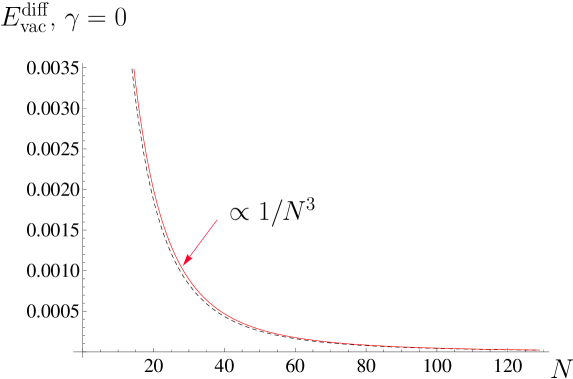
Figure 16: Difference between vacuum energies at $\ell=3$ versus $N$ (dashed line), and its asymptotic approximation (solid line).

Therefore, in the thermodynamic limit the forerunners of the quantum phase transition in the isotropic XX model approach the ground state faster than the ones of the XY model (with $\gamma\neq 0$). Compare figures 13 and 16.

As shown in figure 15, the intersection points of the two vacua (which coincide with the level crossing points $g_{l}(n)$ discussed in section 3) are characterized by a discontinuity of the first derivative for finite size chains. By deriving the energy difference (6hijquvbbbcbdbscrcs), one can show that the discontinuity of the first derivative at the points of level crossing scales like $1/N$; therefore in the thermodynamic limit the divergence of the second derivative vanishes, as for the XY Hamiltonian with $\gamma\neq 0$.

Let us finally consider the points $g=\pm 1$: on one hand they are level crossing points ($g=\pm\sqrt{1-\gamma^{2}}$, $\gamma=0$), on the other hand, following the same criterion introduced for the XY model, they can be considered as forerunners of quantum phase transitions: what happens in this particular case is that these points belong to the ground state already for finite $N$. Another crucial difference between the anisotropic case and the XX model is that, since all Bogoliubov fermions are single, there are $N+1$ points forerunning the quantum phase transition. Thus in the $N\to\infty$ limit they densely fill the interval $[-1,1]$ of $g$ and yield, as one expects [4], a continuous quantum phase transition in this interval.

Conclusions

In this paper we analyzed the XY model with periodic boundary conditions. Being interested in finite size systems, we did not neglect the boundary term which derives from the Jordan-Wigner transformation. In order to diagonalize the Hamiltonian we deformed the discrete Fourier transform with a local gauge coefficient depending on the parity of spins down, anti-parallel to the magnetic field. We then showed that in the Fourier space there are two classes of fermions, single and coupled ones; this distinction is crucial in order to determine the Bogoliubov transformation, which is also gauge dependent. From the expression of the diagonalized Hamiltonian we reinterpreted the ground state and the first excited level of the system as given by a competition between the vacuum energies of the two parity sectors. We finally introduced a criterion to find those values of the magnetic field that can be considered forerunning quantum phase transitions in the thermodynamic limit. They are associated to single Bogoliubov fermions and to the level crossings between physical and unphysical states.

There is considerable interest in the study of entanglement for quantum spin chains, both in view of applications and because of their fundamental interest. See, for example, the results concerning the XX chain [16, 25, 22]. Future activity will focus on the study of the properties of the multipartite entanglement of the ground state in terms of the distribution of bipartite entanglement [26, 27] and on the investigation of the possible connections with quantum phase transitions in the thermodynamic limit.

References

References

- [1] Nielsen M A and Chuang I L 2000 Quantum Computation and Quantum Information (Cambridge: Cambridge University Press)
- [2] Lieb E, Schultz T and Mattis D 1961 Ann. Phys. 16 407
- [3] Pfeuty P 1970 Ann. Phys. 57 79
- [4] Takahashi M 1999 Thermodynamics of One-Dimensional Solvable Models (Cambridge: Cambridge University Press) p 252
- [5] Shastry B S and Sutherland B 1990 Phys. Rev. Lett. 65 243
- [6] Schulz H J and Shastry B S 1998 Phys. Rev. Lett. 80 1924
- [7] Fel’dman E B and Rudavets M G 1999 Chem. Phys. Lett. 311 453
- [8] Osterloh A, Amico L and Eckrn U 2000 Nucl. Phys. B 588 531
- [9] Wootters W K 2001 Quant. Inf. Comp. 1 27
- [10] Amico L, Fazio R, Osterloh A and Vedral V 2008 Rev. Mod. Phys. 80 517
- [11] Wang X 2002 Phys. Rev. A 66 034302
- [12] Kamta G L and Starace A F 2002 Phys. Rev. Lett. 88 107901
- [13] Cao M and Zhu 2005 Phys. Rev. A 71 034311
- [14] Asoudeh M and Karimipour V 2007 Phys. Rev. A 71 022308
- [15] Canosa N and Rossignoli R 2007 Phys. Rev. A 75 032350
- [16] Son W, Amico L, Plastina F and Vedral V 2008 Quantum instability in a quasi-long-range ordered phase Preprint 0807.1602 (quant-ph)
- [17] Osterloh A, Amico L, Falci G and Fazio R 2002 Nature 416 608
- [18] Vidal G, Latorre J I , Rico E and Kitaev A 2003 Phys. Rev. Lett. 90 227902
- [19] Verstraete F, Popp M and Cirac J I 2004 Phys. Rev. Lett. 92 027901
- [20] Roscilde T, Verrucchi P, Fubini A, Haas S and Tognetti V 2004 Phys. Rev. Lett. 93 167203
- [21] Campos Venuti L, Degli Esposti Boschi C and Roncaglia M 2006 Phys. Rev. Lett. 96 247206
- [22] De Pasquale A, Costantini G, Facchi P, Florio G, Pascazio S and Yuasa K 2008 Eur. Phys. J. Special Topics 160 127
- [23] Bratteli O and Robinson D W 1997 Operator Algebras and Quantum Statistical Mechanics (Berlin: Springer) 5.2.1.
- [24] Jordan P and Wigner E 1928 Z Physik 47 631
- [25] Costantini G, Facchi P, Florio P and Pascazio S 2007 J. Phys. A: Math. Theor. 40 8009
- [26] Scott A J 2004 Phys. Rev. A 69 052330
- [27] Facchi P, Florio G, Parisi G and Pascazio S 2008 Phys. Rev. A 77 060304(R)