Escape transition of a polymer chain from a nanotube: how to avoid spurious results by use of the force-biased pruned-enriched Rosenbluth algorithm

Abstract

A polymer chain containing $N$ monomers confined in a finite cylindrical tube of diameter $D$ grafted at a distance $L$ from the open end of the tube may undergo a rather abrupt transition, where part of the chain escapes from the tube to form a “crown-like” coil outside of the tube. When this problem is studied by Monte Carlo simulation of self-avoiding walks on the simple cubic lattice applying a cylindrical confinement and using the standard pruned-enriched Rosenbluth method (PERM), one obtains spurious results, however: with increasing chain length the transition gets weaker and weaker, due to insufficient sampling of the “escaped” states, as a detailed analysis shows. In order to solve this problem, a new variant of a biased sequential sampling algorithm with re-sampling is proposed, force-biased PERM: the difficulty of sampling both phases in the region of the first order transition with the correct weights is treated by applying a force at the free end pulling it out of the tube. Different strengths of this force need to be used and reweighting techniques are applied. Using rather long chains (up to $N=18000$) and wide tubes (up to $D=29$ lattice spacings), the free energy of the chain, its end-to-end distance, the number of “imprisoned” monomers can be estimated, as well as the order parameter and its distribution. It is suggested that this new algorithm should be useful for other problems involving state changes of polymers, where the different states belong to rather disjunct “valleys” in the phase space of the system.

I Introduction

A polymer chain with one end grafted to a non-adsorbing impenetrable surface exists in a mushroom conformation. If it is progressively squeezed by a flat piston of finite radius $L$ from above the conformation gradually changes into a relatively thick pancake. However, beyond a certain critical compression, the chain configuration changes abruptly. One part of the chain forms a stem stretching from the grafting point to the piston edge, while the rest of the segments forms a coiled crown outside the piston, thus escaping from the region underneath the piston. This phenomenon was named the escape transition and has attracted great interest Subra ; Ennis ; Sevick ; Steels ; Milchev99 . An abrupt change from one state to another implies a first order transition. Phase transitions at the level of an individual macromolecule have generic features that are common to all conventional phase transitions in fluids or magnetics. On the other hand, they may be quite unusual, and the conceptual framework that would encompass all the specifics of this class of phase transitions is still being elaborated. A single macromolecule always consists of a finite number of monomers $N$: computer modeling rarely deals with $N$ larger than $10^{5}$  G97 so that finite-size effects in the single-molecule phase transitions are the rule rather than exception. The concept of a phase transition requires that the thermodynamic limit is explored. For a single macromolecule this means the limit of $Na\rightarrow\infty$, while in the specific case of the escape transition it was shown that the appropriate limits are $Na\rightarrow\infty$ and $L\rightarrow\infty$ but $Na/L=const$.

Figure 1: Schematic drawings of a flexible polymer chain of length $N$ grafted to the bottom of the left side of which is open at the right end, of a tube of length $L$ and diameter $D$ at the transition point. As the chain is fully confined in the tube (in an imprisoned state), it forms a sequence of $n_{b}=ND^{-1/\nu}$ blobs in a cigar-like shape, here $\nu$ is the 3D Flory exponent. As one part of the chain escapes from the tube (in an escaped state), it forms a flower-like configuration which consists of a “stem” and a coiled “crown”. By adjusting one of the three parameters $D$, $L$ and $N$, an escape transition occurs. At the transition point $D=D^{*}$, $L=L^{*}$, or $N=N^{*}$, the conformation of a polymer chain is either in an imprisoned state or in an escaped state.

The classical examples of phase transitions in a single macromolecule are the coil-globule and adsorption transitions as well as the coil-stretch transition in a longitudinal flow that have been studied for many years theoretically, experimentally and by computer simulations. A dramatic progress in experimental methods allowing detection and manipulation of individual macromolecules happened in the last decade and includes the AFM manipulations, optical tweezers, high-resolution fluorescent probes Schroeder ; Hugel ; Matsuoka . As for the escape transition in its standard setup, ensuring that the piston is flat and parallel to the grafting surface currently turned out to be a difficult technical problem. The progress in these methods is, however, so rapid and impressive that experimental studies of the escape transition must soon become within reach. Meanwhile the theoretical analysis suggests that the escape transition is extremely unusual in many aspects as compared to conventional phase transitions in fluids or magnetics. First, this is a first-order transition with no phase coexistence, and therefore, no phase boundaries, no nucleation effects, etc. On the other hand, metastable states are well defined up to spinodal lines; they have a clear physical meaning and can be easily visualized. The transition is purely entropy-driven, the energy playing no role at all. Of course, this is a consequence of considering only the excluded volume and hard-wall potentials, and the similar entropy-driven transitions were found in the hard-sphere and hard-rod fluids Allen . Further, the escape transition demonstrates negative compressibility and a van-der-Waals-type loop in a fully equilibrium isotherm: this follows from exact analytical theory and was verified by equilibrium Monte-Carlo simulations. Finally, it was shown that the equation of state (compression force versus the piston separation) corresponding to the escape transition setting is not the same in two conjugate ensembles (constant force and constant separation) giving a unique example of the non-equivalence of statistical ensembles that persists in the thermodynamic limit. Naturally the literature on the subject is quite extensive Skvortsov07 .

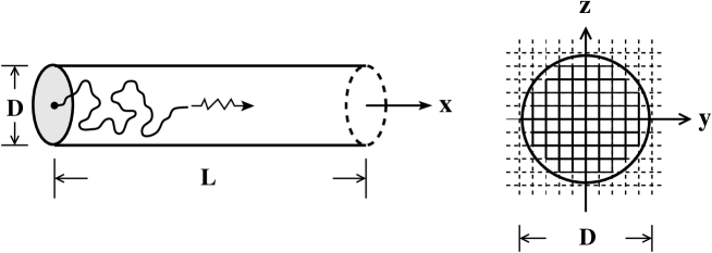
Figure 2: Schematic drawing of a one-end grafted polymer chain growing as a self-avoiding walk inside a finite tube of length $L$ and diameter $D$ along the $x$-direction. The first monomer is located at $(x=0,y=0,z=0)$. Other monomers are allowed to sit on lattice sites of a simple cubic lattice, except for the lattice sites representing the cylindrical walls $\{0\leq x\leq L,y^{2}+z^{2}=D^{2}/4\}$ and the bottom $\{x=0,y^{2}+z^{2}<D^{2}/4\}$.

Yet one more intriguing feature of the escape transition is that it persists in quasi-one-dimensional settings such as a $2d$ chain confined in a strip or a $3d$ chain confined in a tube. The existence of such a transition seems to formally contradict a well-known statement forbidding phase transitions in $1d$ systems Landau . It is also counter-intuitive and goes against a simple blob picture of a chain in a tube Daoud ; Kremer ; Milchev94 ; Sotta ; Yang , which suggests that squeezing the tube would result in progressively pushing out the chain segments very much alike the toothpaste. Predictions of the naive blob picture were discussed in the context of a $2d$ chain confined in an open strip of finite length Hsu07 . It was shown that they contradict both the MC simulations with PERM and a more sophisticated analytical theory. There are two reasons that prompt a revisiting of the escape transition in one-dimensional geometry. First, the strip confinement of a $2d$ chain is rather exotic and difficult to realize experimentally. On the other hand, confining a real chain in a nanotube with the diameter much smaller than the chain gyration radius in solution is experimentally feasible. Well-calibrated nanochannels are being produced by lithographical methods with the width in the range between $30$ and $400$ nm Reisner . Partially escaped configurations appear also in situations where a long polymer chain is translocating through a pore in a relatively thick membrane Randel . From the point of view of computational physics, in general, first-order transitions and inhomogeneous polymer conformations are particularly very difficult to cope with; we have encountered these difficulties in the study of a $2d$ escape transition Hsu07 , which motivated the development of a new variant of the algorithm PERM, force-biased PERM. This new algorithm is specifically suited for exploring well-separated regions in the phase space.

The aim of our paper is twofold: (1) we demonstrate unambiguously the existence of a first-order escape transition in the setting of a real $3d$ polymer confined in a tube; (2) we present the force-biased PERM, and show its advantages in comparison with PERM, or more precisely, PERM with $k$-step Markovian anticipation.

The paper is organized in a non-traditional way. In Sec. II, we present three different scenarios of the escape transition and the simulational model. In Sec. III and Sec. IV, we first present the results of the Monte Carlo (MC) simulations with PERM and force-biased PERM. These include a collection of equilibrium characteristics and lateral size distribution for a chain in an infinite tube (without the possibility of escape) in comparison with the scaling predictions. Then we discuss the characteristics of the escape transition and its smoothing due to the finite-size effects. In Sec. V. and VI, we explain the idea and the implementation of force-biased PERM, and give a clear demonstration of a failure of PERM in application to the escape transition. We also present a glimpse of the computational technique whereby the artifacts of the method could lead to misleading conclusions concerning the nature of the transition in the thermodynamic limit, and discuss ways to detect the possible flaws in the simulation results. Finally, a summary is given in Sec. VII.

II Escape transition scenarios and simulational model

The escape transition of an end-attached polymer chain inside a confined space may be triggered by changing any of the following parameters:

1. the piston separation Subra ; Ennis ; Sevick ; Steels ; Milchev99 or the tube diameter Hsu07 which control the degree of confinement;

2. the distance from the grafting point inside the confined space to the edge of the opening (this would be the piston radius $R$ in a traditional escape setting Subra ; Ennis ; Sevick ; Steels ; Milchev99 or the tube length $L$)

3. the chain contour length, $Na$, where $a$ is the segment length. $a$ is set to $1$ throughout the paper hereafter.

Three corresponding scenarios of a polymer chain escaping from a tube are schematically illustrated in Fig. 1, although not all of them can find a reasonable experimental implementation. In a classical escape setting, the confinement width is easily changed by moving the piston, while the piston radius was assumed to be a constant Subra ; Ennis ; Sevick ; Steels ; Milchev99 . For a tube, changing its diameter $D$ is much more difficult to realize experimentally, but the distance from the grafting point to the tube opening, $L$, can be changed naturally by moving a bead with a chain end grafted to it, inside the tube. Chopping the tube off in thin slices is another way of changing $L$ albeit rather artificial. Finally, one can envisage a mechanism which leads to a gradual change in the chain contour length (this may involve ferments that cut a molecule). From the point of view of PERM, the scenario of gradual growing a chain is the easiest one to be implemented. We study single flexible polymer chains of length $N$ with one end grafted to the center of the bottom of a finite tube of length $L$ and diameter $D$ under good solvent conditions. They are described by a self-avoiding random walk (SAW) of $N$ steps on a simple cubic lattice as shown in Fig. 2 with the restriction that monomers are forbidden to be located on the surface of the cylinder. Taking the bottom center at the origin $(x,y,z)=(0,0,0)$ with the first monomer fixed there, and the tube axis along the $x$-direction, monomers are not allowed to be located on the lattice sites $0\leq x\leq L$, $y^{2}+z^{2}=D^{2}/4$ and $x=0$, $y^{2}+z^{2}<D^{2}/4$. The idea of using a half-opened tube and a chain with one end grafted to its bottom is that with a chain growth algorithm the chain has to grow either along $+x$-direction or $-x$-direction as $N^{\nu}\sim D$, and the partition sum just differs by a constant comparing to the case of unfixed chain ends Hsu03 . However, the scaling behaviour of confined polymer chains remains the same for this simplified model.

III Confined chains in an infinite tube

The properties of a single macromolecule confined in a tube have been studied extensively for decades, both by analytical theory and by numerical simulations for various models of flexible and semi-flexible chains Daoud ; Kremer ; Milchev94 ; Sotta ; Yang . For a homogeneous confined state there are scaling predictions Daoud concerning various chain characteristics which were tested by MC simulations.

The scaling laws are well known Daoud ; deGennes for a fully confined polymer chain of chain length $N$ in a tube of length $L$ and diameter $D$ under a good solvent condition. One should expect a crossover between a weak confinement region $1\ll N^{\nu}\ll D$ ($\nu$ is the Flory exponent), where the chain forms a three-dimensional random coil, and a strong confinement region $1\ll D\ll N^{\nu}$, where the chain forms a quasi-one dimensional conformation (a long cigar-shaped object which is described as a chain of spherical blobs in a blob picture).

For a grafted polymer chain confined in a very wide tube, $D>>N^{\nu}$, since the chain stays essentially unaffected by the existence of the cylindrical hard surface, i.e., there is no repulsive interaction between the chain and the cylindrical hard surface, the system is simplified to be in the situation that a polymer chain is with one end grafted to a repulsive wall in a good solvent. Using a self-avoiding walk (SAW) of $N$ steps on a simple cubic lattice with a constraint that $x>0$, it is well known that in the limit of $N\rightarrow\infty$ the end-to-end distance scales as

$$R_{N}\sim N^{\nu}$$ (1)

with $\nu=0.58765(20)$ Hsu04mac , which shows the same behavior as in the bulk.

A scaling ansatz of the end-to-end distance along the direction parallel to the tube axis, $R_{||}(N,D)$, for the cross-over between these two regimes $1<<N^{\nu}<<D$ and $1<<D<<N^{\nu}$ is

$$R_{\parallel}(N,D)=R_{N}\Phi_{R}(R_{N}/D)\;,$$ (2)

where $R_{N}$ is given by Eq. (1) and requesting that for large $N$ the parallel linear dimension is proportional to $N$ yields for the function $\Phi_{R}$ the limiting behaviours

$$\Phi_{R}(\eta)=\left\{\begin{array}[]{ll}const&{\rm for}\enspace\eta\rightarrow 0\\ \eta^{-1+1/\nu}&{\rm for}\enspace\eta\rightarrow\infty\end{array}\right.$$ (5)

with $\eta=N^{\nu}/D$. The same scaling ansatz is also expected for $R_{\perp}(N,D)$,

$$R_{\perp}(N,D)=R_{N}\Psi_{R}(R_{N}/D)\;,$$ (6)

and requesting that for large $N$ the perpendicular linear dimension is independent of $N$ yields for the function $\Psi_{R}$ the limiting behaviours

$$\Psi_{R}(\eta)=\left\{\begin{array}[]{ll}const&{\rm for}\enspace\eta\rightarrow 0\\ \eta^{-1}&{\rm for}\enspace\eta\rightarrow\infty\end{array}\right.\;.$$ (9)

Figure 3: Rescaled rms end-to-end distance parallel to the tube, $R_{||}(N,D)/N^{\nu}$, plotted against $\eta=N^{\nu}/D$. The data collapse is achieved by Eq. (2) and corrections to scaling are not visible in a log-log scale. The inset shows the log-log plot of $\Delta R_{||,\infty}=\lim_{N\rightarrow\infty}R_{\parallel}(N,D)/N$ versus $D$. The dashed line is $0.93D^{1-1/\nu}$.

Figure 4: Rescaled rms end-to-end distance perpendicular to the tube, $R_{\perp}(N,D)/N^{\nu}$, plotted against $\eta$. The data collapse is achieved by Eq. (6) and corrections to scaling are not visible in a log-log scale. The inset shows the log-log plot of $R_{\perp,\infty}=\lim_{N\rightarrow\infty}R_{\perp}(N,D)$ versus $D$. The dashed line is $0.295D$.

In order to obtain the full functions $\Phi_{R}(\eta)$, $\Psi_{R}(\eta)$ interpolating between the quoted limits, we apply MC methods. For the MC simulations, we use the chain growth algorithm PERM with $k$-step Markovian anticipation and simulate single fully confined chains of chain lengths $N$ up to $44000$, and tube diameters $D$ up to $97$. According to the cross-over scaling ansatz, Eqs. (2) and (6), we plot the rescaled average root mean square (rms) end-to-end distances parallel and perpendicular to the tube axis, $R_{\parallel}/N^{\nu}$ and $R_{\perp}/N^{\nu}$, against $N^{\nu}/D$ in Fig. 3 and 4, respectively. A nice data collapse is indeed seen in both figures. For a further check of the scaling law depending on $D$ in the regime of $N^{\nu}>>D$ (the strong confinement limit) and giving a precise estimate of the prefactor, we estimate the asymptotic ratios between $R_{\parallel}$ and $N$, i.e. $\Delta R_{\parallel,\infty}=\lim_{N\rightarrow\infty}R_{\parallel}(N,D)/N$. and the asymptotic value of $R_{\perp}$ as $N\rightarrow\infty$, i.e. $R_{\perp,\infty}=\lim_{N\rightarrow\infty}R_{\perp}(N,D)$, for various diameters $D$. Results of $\Delta R_{\parallel,\infty}$ and $R_{\perp,\infty}$, plotted against $D$ are shown in the inset of Fig. 3 and Fig. 4, respectively. In the thermodynamic limit $N\rightarrow\infty$, $R_{\parallel}$ and $R_{\perp}$ scale as follows

$$R_{\parallel}=\left\{\begin{array}[]{ll}0.85(2)N^{\nu}&{\rm for}\enspace D>>N^{\nu}>>1\\ 0.93(2)ND^{1-1/\nu}&{\rm for}\enspace N^{\nu}>>D>>1\end{array}\right.\;,$$ (12)

and

$$R_{\perp}=\left\{\begin{array}[]{ll}0.89(2)N^{\nu}&{\rm for}\enspace D>>N^{\nu}>>1\\ 0.295(8)D&{\rm for}\enspace N^{\nu}>>D>>1\end{array}\right.\;.$$ (15)

Due to the confinement of the chain in a tube, in Eq. (15) we see that $R_{\perp}$ is only dependent on the tube diameter $D$ but independent of $N$ in the strong confinement regime. In the very weak or no confinement regime, the estimate of the ratio between the average mean square end-to-end distances in both directions, $(R_{\parallel}/R_{\perp})^{2}\approx 0.91(8)$ is in good agreement with the result in Ref. Grass05 ($<z_{N}^{2}>/<x_{N}^{2}+y_{N}^{2}>=0.938(2)$ as $N\rightarrow\infty$), although our chain lengths in the region $D>>N^{\nu}>>1$ are much shorter.

It is also remarkable that the crossover between both limits in Eqs. (12), (15) is rather sharp and not spread out over a wide regime in the scaling variable $N^{\nu}/D$. For $R_{||}$ this crossover occurs for $N^{\nu}/D\approx 1$ but for $R_{\perp}$ it occurs near $N^{\nu}/D\approx 0.4$, however.

An additional bonus of the PERM algorithm G97 , as compared to standard “dynamic” MC algorithms as applied in Kremer ; Milchev94 is that it yields the free energy. The excess free energy relative to a one-end grafted random coil, $F(N,D)=-\ln\left[Z(N,D)/Z^{(1)}_{N}\right]$, where $Z_{N}^{(1)}\sim\mu^{-N}N^{\gamma^{(1)}-1}$ with $\mu=0.21349098(5)$ and $\gamma^{(1)}=0.6786(12)$ Grass05 , is a constant in the regime $D>>N^{\nu}>>1$ while it is proportional to the number of blobs, $n_{b}=ND^{-1/\nu}$, in the unit of $k_{B}T$ in the regime $N^{\nu}>>D>>1$. Therefore, we can rewrite the scaling law as follows,

$$\frac{F(N,D)}{ND^{-1/\nu}}=\left\{\begin{array}[]{ll}const\;\eta^{-1/\nu}&{\rm for}\enspace\eta\rightarrow 0\\ const^{\prime}&{\rm for}\enspace\eta\rightarrow\infty\end{array}\right.$$ (18)

As expected, results of the rescaled free energy in Fig. 5 also show the nice data collapse of the cross-over behavior predicted by Eq. (18). In the strong confinement regime, the imprisoned free energy scaled as follows,

$$F_{\rm imp}(N,D)=5.40(2)n_{b}\;.$$ (19)

Again the crossover is very sharp, occurring near a value $N^{\nu}/D\approx 0.4$ of the scaling variable.

Figure 5: Rescaled free energy relative to a one-end grafted random coil, $F(N,D)/(ND^{-1/\nu})$ in a log-log scale. The data collapse is achieved by Eq. (18). The inset shows the log-log plot of $\Delta F_{{\rm imp},\infty}=\lim_{N\rightarrow\infty}F(N,D)/N$ versus $D$. The dashed line is $5.40D^{-1/\nu}$.

According to the scaling theory Daoud , the free energy in the strong confinement limit is always proportional to the number of blobs, $n_{b}$. In the special case of quasi-1d confinement (a tube for $3d$ chains or a strip for $2d$ chains) the average end-to-end distance is proportional to $n_{b}D$, so that the ratio $FD/R_{\parallel}$ is independent of both $N$ and $D$. Physically, this ratio gives an estimate for the free energy of confinement per blob in $k_{B}T$ units. The question of whether this ratio is model-dependent or universal was addressed by Burkhardt and Guim Burkhardt . Using field-theoretical methods and the equivalence of self-avoiding walks and the $n$-vector model of magnetism in the limit of $n\rightarrow 0$ they have shown that this ratio (which we denote in the following as the Burkhardt amplitude $A_{B}$) is indeed universal. Extrapolating finite-size transfer-matrix results for the case of repulsive walls in $d=2$ they obtained a numerical estimate of $A_{B2}\approx 2.10\pm 0.01$. Although MC simulation data for $2d$ SAWs confined in a strip with hard walls were obtained a few years ago, no direct comparison to the theoretical prediction was made at the time. The MC data of Hsu and Grassberger give $R_{\parallel}\approx 0.915ND^{-1/3}$ Hsu03 and $F=1.944(2)ND^{-4/3}$ Hsu07 which results in $A_{B2}\approx 2.12(4)$ in excellent agreement with field-theoretical calculations. For a $3d$ chain in a tube the Burkhardt amplitude must be also universal although no numerical estimates were ever produced. From our MC results, Eq. (12) and (19), it gives $A_{B3}\approx 5.79(6)$. It would be interesting to check this value using other simulation models.

It was proposed and checked numerically for short polymer chains in Ref. Sotta that the distribution for the gyration radius $r_{g}$ along the tube axis can be presented as a sum of two terms:

$$\ln P(r_{g}|N,D) = N(D/a)^{-1/\nu}A\left[u^{-\alpha}+Bu^{\delta}\right]\;,$$ (20)

where $\alpha$ and $\delta$ are linked to the space dimension $d$ and the Flory exponent $\nu$ by $\alpha=\left(\nu d-1\right)^{-1}$ and $\delta=\left(1-\nu\right)^{-1}$, and $u=(r_{g}/Na)(D/a)^{-1+1/\nu}$ is the segment volume concentration expressed as a function of the gyration radius and the confinement geometry. The parameters A and B are model-dependent numerical coefficients of order unity, which do not depend on $N$ or $D$.

From our MC simulations, we found that the above formula has to be corrected by an additional $r_{g}$-independent term, i.e.

$$\ln P(r_{g}|N,D)=N(D/a)^{-1/\nu}A\left[u^{-\alpha}+Bu^{\delta}+C\right]\;.$$ (21)

Results of the rescaled distribution $\ln(P(r_{g}|N,D)/P(r_{m}|N,D))/ND^{-1/\nu}$ plotted against $r_{g}/(ND^{1-1/\nu})$ for $N=5000$, and $10000$, and for $D=25$, $33$, and $49$ are shown in Fig 6. Here the radius of gyration $r_{g,m}$ corresponds to the maximum of the distribution $P(r_{g}|N,D)$. Near $r_{g,m}$, we see a very nice data collapse, and the rescaled distribution can be described by Eq. (21) with $A=-0.185$, $B=76.757$, and $C=-8.784$ very well. Thus we conclude that Eq. (21), even if it is not exact, at least is a very good numerical approximation to the actual distribution function. In Fig. 7, we check that the results for the end-to-end distance distribution $P(r_{\parallel}|N,D)$ can be also described by the same function {Eq. 21} with $A=-0.953$, $B=0.801$, and $C=-1.771$.

Figure 6: Rescaled distribution $\ln(P(r_{g}|N,D)/P(r_{g,m}|N,D))/(ND^{-1/\nu})$ plotted against $r_{g}/ND^{1-1/\nu}$ for various values of $N$ and $D$. The radius of gyration $r_{g,m}$ corresponds to the maximum of the distribution $P(r_{g}|N,D)$. Near $r_{g,m}$, $f(x)=A(x^{-\alpha}+Bx^{\delta}+C)$ with $A=-0.185$, $B=76.757$, and $C=-8.784$ gives the best fit of the data, here $x=r_{g}/(ND^{1-1/\nu})$.

Figure 7: Rescaled distribution $\ln(P(r_{\parallel}|N,D)/P(r_{\parallel,m}|N,D))/(ND^{-1/\nu})$ plotted against $r_{\parallel}/ND^{1-1/\nu}$ for various values of $N$ and $D$. The end-to-end distance $r_{\parallel,m}$ corresponds to the maximum of the distribution $P(r_{\parallel}|N,D)$. Near $r_{g,m}$, $f(x)=A(x^{-\alpha}+Bx^{\delta}+C)$ with $A=-0.953$, $B=0.801$, and $C=-1.771$ gives the best fit of the data, here $x=r_{\parallel}/(ND^{1-1/\nu})$.

IV Single polymer chains escape from a nanotube

We simulate 3D SAW and BSAWs starting at the grafting point of the tube with length $L=200$, $400$, $800$, and $1600$, and diameter $D=17$, $21$, $25$ and $29$. Depending on the chosen size of $L$ and $D$, the total chain length is varied from 1400 to 18000 in order to cover the transition regime. Results of the free energy relative to a one-end grafted random coil for $L=800$ and $L=1600$ are shown in Fig. 8. It is clear that there are two branches of the free energy. For a fixed diameter $D$ we see that initially the free energy increases linearly with the chain length $N$, but as $N$ exceeds a certain value, the chain escapes from the tube, a sharp crossover behavior from an imprisoned state to an escaped state is indeed seen. Values of the excess free energy of the chain in an escaped state, $F_{\rm esc}(N,L,D)$, are determined by the horizontal curves shown in Fig. 8, which are independent of $N$. Results of $F_{\rm esc}(N,L,D)$ for various values of $L$ and $D$ are presented in Fig. 9, where we obtain

$$F_{\rm esc}(N,L,D)=4.23(7)L/D$$ (22)

Figure 8: Free energy relative to a one-end grafted chain, $F(N,L,D)=-\ln[Z(N,L,D)/Z_{N}^{(1)}(D)]$, plotted against $ND^{-1/\nu}$.

Figure 9: The log-log plot of the excess free energy of the escaped chain, $F_{\rm esc}(N,L,D)$, plotted against $L/D$ for various values of $L$ and $D$. The dashed line is $4.23L/D$ and gives the best fit of the data.

Figure 10: Results of the transition points obtained by estimating the intersection points of the two branches shown in Fig. 8. The dashed line is $0.785L/D$ and gives the best fit of the data.

According to the requirement that the free energies of polymer chains in both imprisoned and escaped states should be the same at the transition point, the transition point is therefore determined by equating Eq. (19) and Eq. (22). We obtain the relation between $L$, $N$, and $D$ at the transition point, i.e.,

$$(N/L)_{\rm tr}=0.78(2)D^{1/\nu-1}\;.$$ (23)

One can also estimate $ND^{-1/\nu}$ at the transition point directly from Fig. 8 for fixed tube length $L$ and tube diameter $D$. In Fig. 10 we plot $ND^{-1/\nu}$ against $L/D$. The best fit for the data given by the straight line is $ND^{-1/\nu}=0.785(10)L/D$ which is in perfect agreement with Eq. (23).

Figure 11: Average end-to-end distance divided by $L$, $R_{||}/L$, plotted against $N/L$ for various values of $L$ and $D$. The rounding of the transition is due to the finiteness of the chain length $N$.

Figure 12: Average fraction of imprisoned number, $N_{\rm imp}/N$, plotted against $N/L$ for various values of $L$ and $D$. The rounding of the transition is due to the finiteness of the chain length $N$.

In order to understand the conformational change of the polymer chains from an imprisoned state to an escaped state, in Fig. 11 we show the results of the end-to-end distance parallel to the tube axis normalized by the tube length $L$, $R_{||}/L$, versus $N/L$. As the chain is still in the strong confinement regime, $R_{||}$ increases linearly with $N$, showing that the chain is stretched. Beyond a certain value of $N/L$, there is a jump in each curve, showing the chain undergoes an escape transition, i.e., one part of the chain escapes from the tube (see Fig. 1). Obviously, we see that the transition becomes sharper as the tube length $L$ increases or the tube diameter $D$ decreases. The pronounced jump indicates that the transition is first-order like. A similar jumpwise change is also expected for the average number of imprisoned monomers, $N_{\rm imp}$. In Fig. 12, we plot the fraction of imprisoned monomers, $N_{\rm imp}/N$, versus $N/L$ for various values of $L$ and $D$. It is indeed seen that there exist jumps from $N_{\rm imp}/N=1$ while the chain is confined completely to $N_{\rm imp}/N\approx 3/4$ as $N/L$ increases, and the rounding of the transition is due to the finite size effect. In the problem of escape transition, the order parameter is defined by the stretching degree of the confined segments of polymer chains. As the chain is in an imprisoned state, $s=r/N$ where $r$ is the instantaneous end-to-end distance of the confined chain along the tube axis, while as the chain is in an escaped state, $s=L/n$ where $n$ is the imprisoned number of monomers (number of monomers in the stem) Klushin04 . Results of the average order parameter $S=<s>$ against $N/L$ are presented in Fig. 13. An abrupt jump from $S_{\rm imp}$ to $S_{\rm esc}$ is developed at the transition point in Fig. 13 as the system size $L$ increases for each data set of a given value of $D$. Since it is difficult to give a precise estimate of the transition point directly from those results shown in Fig. 11-13, we use a different strategy by plotting a straight line with $N/L=0.785D^{1/\nu-1}$ for each $D$. We see that the straight lines do go through the intersection point for a fixed value $D$ (results are not shown).

Figure 13: Average order parameter $S$ plotted against $N/L$ for various values of $L$ and $D$. The rounding of the transition is due to the finiteness of the chain length $N$.

Finally, results of the distribution function of the order parameter, $P(N,L,D,s)$, are presented in Fig. 14 for $L=1600$ and $D=17$ near the transition point. For our simulations, the distribution function $P(N,L,D,s)$ is given by properly normalized accumulated histograms of the order parameter $s$, namely $\sum_{s}P(N,L,D,s)=1$ (see Sec. V). We see the bimodal behavior of the distribution functions as one should expect for the first-order transition near the transition point. At the transition point $(N/L)_{\rm tr}\approx 5.7$, the two peaks are of equal height. Below the transition point chains are in favor of staying in an imprisoned state, while above the transition point chains stay in an escaped state.

Figure 14: Distribution functions of the order parameter $P(N,L,D,s)$ vs. $s$ near the transition point for $L=1600$ and $D=17$. . The distribution is normalized by choosing $\sum_{s}P(N,L,D,s)=1$. A constant $\Delta$ is added to distinguish between different curves.

V Force-biased PERM

According to the predictions of the Landau free energy approach in three dimensions at the escape transition point, the magnitude of the jumps of the end-to-end distance, the order parameter, and the fraction of imprisoned number of monomers should be much more prominent than that for the 2d case described in our previous work Hsu07 . There, polymer chains were described by 2d SAW on a square lattice with the constraint that chains are confined in finite strips. In order to suppress dense configurations and sample more relatively open chain configurations, we employed the algorithm PERM with $k$-step Markovian anticipation G97 ; Hsu03 to study the problem of 2d escape transition. However, this method is very efficient for generating homogeneous configurations of very long polymer chains in the imprisoned state not only for the 2d case but also for the 3d case which will be presented in the next section, while it fails with producing inhomogeneous flower-like configurations in the escaped state. The difficulty was already noticed in Ref. Hsu07 by the disappearance of jumps in the thermodynamic limit and the lack of data for describing the Landau free energy as a function of the order parameter $s$ in an escaped state for larger systems. Clearly, it becomes a more serious problem when the same sampling method and model are applied to the study of polymer chains escaping from a tube. Our test run showed that for a fixed diameter $D$ the transition occurs much later (if we choose $N/L$ as a control parameter) and the magnitude of the jump decreases as the tube length $L$ increases (see Fig. 15). One could imagine that in the thermodynamic limit of $N\rightarrow\infty$ and $L\rightarrow\infty$, the conformation change becomes continuous. However this conjecture is based on the artifacts due to the inefficiency of the original chosen model and method.

A new strategy for generating sufficient samplings of the flower-like configurations in the phase space is proposed as follows: We first apply an extra constant force along the tube to pull the free end of a grafted chain outward to the open end of the tube as long as the chain is still confined in a tube, and release the chain once some segments of it is outside the tube. By varying the strength of the force, we obtain configurations in the escaped state with various stretching degree of monomer segments (stems) which are still confined in a tube. Finally the contributions for the escaped states are given by properly reweighting these configurations to the case without applying extra forces. Now a partially stretched polymer in a good solvent is described by a biased SAW (BSAW) with finite cylindrical geometry confinement. The stretching is denoted by a factor $b=\exp(\beta aF)$ where $a$ is the lattice constant, $F$ is the stretching force, and $\beta=1/k_{B}T$. For our simulations, $a$ and $\beta$ are rescaled as units of length and inverse energy, respectively. Both are set to $1$ in the simulations. The partition sum of a BSAW of $N$ steps is, therefore,

$$Z_{b}(N,L,D)=\sum_{walks}b^{\Delta x}$$ (24)

with

$$b=\left\{\begin{array}[]{ll}\geq 1&,\enspace 0<x\leq L\;,y^{2}+z^{2}<D\\ 1&,\enspace{\rm otherwise}\,{\rm(SAW)}\end{array}\right.$$ (27)

here $\Delta x=x_{N}-x_{0}$ is the displacement (in units of a lattice constant) of the end-to-end vector onto the direction of ${\bf F}$ (along the tube axis). The first monomer is located at $x_{0}=0$ as shown in Fig. 2. Based on the algorithm PERM, polymer chains are built like random walks by adding one monomer at each step and each configuration carries its own weight which is a product of those weight gains at each step, i.e. $W(N)=\Pi_{j=1}^{N}w(j)$ with $w(j)=b^{(x_{j}-x_{j-1})}$ and $w(j=0)=1$ in the current case (cf. Eq. (24)). It has the advantage that one can estimate the partition sum directly as given by,

$$\hat{Z}_{b}(N,L,D)=\frac{1}{M_{b}}\sum_{\{{\cal C}_{b}\}}W_{b}({\cal C}_{b})$$ (28)

here ${\cal C}_{b}$ denotes a configuration of a BSAW of $N$ steps, confined in a finite tube of length $L$ and diameter $D$, $M_{b}$ is the total trial configurations, and $W_{b}({\cal C}_{b})=W_{b}(N,L,D)$ is the total weight of obtaining the configuration ${\cal C}_{b}$. Thus, each configuration of a BSAW with the stretching factor $b_{k}$ contributes a weight $W^{(k)}(N,L,D)$ after re-weighting to compensate for the bias introduced earlier as

$$W^{(k)}(N,L,D)=\left\{\begin{array}[]{ll}W_{b_{k}}(N,L,D)/b_{k}^{x_{N}-x_{0}}\;,&x_{N}\leq L\\ W_{b_{k}}(N,L,D)/b_{k}^{L}\;,&x_{N}>L\end{array}\right.\;,$$ (29)

here index $k$ labels runs with different values of the stretching factor $b$.

Combining data runs with different values of $b$ the average value of any observable $\cal{O}$ is given by

$$<{\cal O}>=\frac{\sum_{k}\sum_{config.\in{\cal C}_{b_{k}}}O({\cal C}_{b_{k}})W^{(k)}(N,L,D)}{\sum_{k}\sum_{config.\in{\cal C}_{b_{k}}}W^{(k)}(N,L,D)}$$ (30)

and the estimate of the partition sum

$$Z(N,L,D)=\frac{1}{M}\sum_{k}\sum_{config.\in{\cal C}_{b_{k}}}W^{(k)}(N,L,D)$$ (31)

here $M$ is the total number of trial configurations.

The distribution of the order parameter, $P(N,L,D,s)\propto H(N,L,D,s)$, is obtained by accumulating the histograms $H(N,L,D,s)$ of $s$, where $H(N,L,D,s)$ is given by,

$$H (N,L,D,s)$$ (32)

$$= \frac{1}{M}\sum_{k}H^{(k)}(N,L,D,s)$$

$$= \frac{1}{M}\sum_{k}\sum_{config.\in{\cal C}_{b_{k}}}W^{(k)}(N,L,D,s^{\prime})\delta_{s,s^{\prime}}$$

and the partition sum of polymer chains confined in a finite tube can be written as

$$Z(N,L,D)=\sum_{s}H(N,L,D,s)$$ (33)

in accordance with Eq. (31).

VI Comparison of results by old and new algorithm

Here we are going to show some of the technical details of simulations by PERM and the resulting problem. We present the spurious results obtained by PERM without force biases in detail and the far-reaching conclusions they could lead to. The whole situation is of considerable methodological and pedagogical value. We also discuss some general ways to avoid the pitfalls and discriminate between authentic and spurious data.

VI.1 Results without force biases: new phase transition physics suggested?

Let us focus on the results of the average end-to-end distance $R_{\parallel}/L$. Using the algorithm PERM with $k$-step Markovian anticipation as in our previous work ($2d$ escape transition) Hsu07 , we present the data of $R_{\parallel}/L$ as a function of the reduced chain length parameter $N/L$ for $D=21$ in Fig. 15. Each curve corresponds to a fixed tube length $L$. With increasing the system size, i.e. increasing $L$ from $L=200$ to $L=1600$, the systematic change of the curves describes the approach to the thermodynamic limit. The data points fall on smooth curves without much statistical scattering, and the curves themselves suggest a systematic trend as $L$ increases. It is clear that for each $L$ the chain size experiences a sharp increase at some value of $N/L$. The sharpness of the curves increases to some extent as the system size increases near the transition point, which is not unexpected if one suspects a first-order transition to be involved. The transition point of a finite system can be estimated, and a shift of its position with increase in $L$ is obvious. Thus one is immediately tempted to extrapolate the transition point to $L\rightarrow\infty$, which is pointed by an arrow in Fig. 15. Simultaneously, the magnitude of the jump is also changing systematically which calls for another extrapolation. This extrapolation shows that in the thermodynamic limit the jump vanishes (the long dashed line in Fig. 15.) Overall, this suggests a sophisticated and weak first-order transition with finite-size effects that disappears in the thermodynamic limit. This is in agreement with the intuitive picture of a chain overgrowing and escaping out of the tube opening without any jumps and also follows the conventional blob picture. Further analysis would have to reconcile several conflicting findings. At the extrapolated transition point, the free energy still has a discontinuity in the slope leaving the signature of a first-order transition. On the other hand, the extrapolated curve of $R_{\parallel}/L$ versus $N/L$ also acquires a discontinuity in the slope suggesting a continuous transition. A thoughtful investigator would recall the statement about impossibility of phase transitions in $1d$ systems. However, at the transition point ($R_{\parallel}=L$), the chain starts leaving the tube and claims back (at least partially) its three-dimensional nature! Overall, the picture of the phenomenon is very rich and thought-provoking. The only curve that is slightly outside the general systematic trend corresponds to $L=200$. However, this can be clearly attributed to the stronger finite-size effect.

Figure 15: Average end-to-end distance divided by $L$, $R_{||}/L$, plotted against $N/L$ for various values of $L$ and $D=21$. Results are obtained by PERM without force biases. The transition point indicated by the arrow is the intersection between the extrapolated curve (long dashed curve) and the curve $R_{||}/L=1$.

Figure 16: Average end-to-end distance divided by $L$, $R_{||}/L$, plotted against $N/L$ for $L=200$ and $600$, and $D=21$. Results are obtained by PERM with (new) and without (old) force biases. The true transition point is indicated by an arrow.

Results obtained by PERM with and without force biases for $L=200$ and $1600$, for $D=21$, and for the chain length $N$ which is large enough to cover the transition regions are shown in Fig. 16 by symbols and curves respectively for comparison. It is clear that for the smaller system, $L=200$, both algorithms give the same results. In contrast to this for $L=1600$ the new algorithm produces a very different curve that does not show a shift of the transition point (nor a decrease in the magnitude of the jump). The true transition point is indicated by an arrow and is as far as about $25\%$ away from the presumed value obtained by extrapolating data to the thermodynamic limit without force biases. In short, the new algorithm confirms that the escape transition is a normal first-order transition with all the expected finite-size effects which include (approximate) the crossing of the curves for different size without a systematic shift and sharpening of the transition with increasing $L$.

(a)      (b) (c)      (d)

Figure 17: Histograms of the order parameter $P(N,L,D,s)$ vs. $s$ near the transition point $(N/L)_{\rm tr}$ for $D=21$ and various values of $L$. The values of $N/L$ are (a) $6.9$, (b) $6.8$, (c) $6.7$, and (d) $6.7$. The distribution is normalized by choosing $\sum_{s}P(N,L,D,s)=1$. The left and right branches correspond to chains in the imprisoned state and escaped states respectively.

VI.2 How to avoid spurious results?

The question posed is of a very general nature that any researcher has to address again and again in various situations. As far as simulated systems undergoing phase transitions are concerned, the best answer that we could come up with is related to the careful analysis of the distribution functions of the order parameter. Here we do not address the question of how to define the order parameter for a particular phase transition. In the case of the escape transition, it was shown in Sec. IV that the order parameter should describe the stretching of the confined segments of a chain, $s=r/N$ for the confined state, and $s=L/n$ for the escaped state. It is intuitively clear that the stretching degree is stronger, i.e., the value of $s$ is larger, for a fully confined chain (in an imprisoned state) than that for a partially confined chain (in an escaped state).

Far from the transition point the distribution function of the order parameter $P(N,L,D,s)$ is unimodal but near the transition point it has a bimodal form as shown in Fig. 14 and Fig. 17. As the system size increases, i.e. $L$ increases for a fixed vale of $D=21$, the shape of $P(N,L,D,s)$ changes systematically. At the transition point the two peaks are of equal height and the depth of the gap between them increases with $L$. For $L=200$ the bimodal behavior of the distribution function $P(N,L,D,s)$ is developed by both algorithms (Fig 17a). A more close inspection shows that using PERM without force biases there is a cut-off at large $s$ although the maxima is traced very confidently. The cut-off appears earlier as $L$ increases and the problem of developing a right-hand maximum becomes progressively severe. Already for $L=800$ the branch of the distribution function corresponding to the escaped state is completely cut off. For $L=1600$ even the full description of the confined state is lost, although the vicinity of the maximum is reproduced very fairly (here the difference between the old and the new method is only due to normalization). A deficient sampling leads to spurious behavior of the equilibrium average. Since the problem is clearly related to poor samplings of strongly stretched states, introducing the force biased strategy that enriches stretched conformations is a natural improvement of the algorithm PERM.

Even if the correct distribution function was not available, the systematic changes in the shape of the distribution function obtained without force biases ring the alarm bell: the initially smooth bimodal distribution function is being progressively and forcibly cut off which does not correspond to any reasonable physical picture. This is a very strong indication that the algorithm experiences severe difficulties in sampling the relevant portions of the phase space. Once these portions are identified, a reasonable recipe for enriching the relevant set of configurations could be normally introduced. To finalize, we stress that following the behavior of the distribution functions with the increase in the system size is a powerful test of the quality of results.

VII Summary

In this paper, we have shown that with the force-biased PERM we are able to produce sufficient samplings for the configurations in the escaped regime for the 3d escape problem. It solves the difficulty of getting inhomogeneous flower-like conformations mentioned in the 2d escape transition Hsu07 . As predicted by the Landau theory approach, we indeed see rather pronounced jumps in the quantities of the end-to-end distance, the fraction of imprisoned number of monomers, and the order parameter. These jumps become sharper as the tube length $L$ increases or the tube diameter $D$ decreases, indicating the transition is a first-order like. The occurrence of an abrupt change of the slope of the free energy gives the precise estimate of the transition point for the polymer chain of length $N$ confined in a finite tube of length $L$ and diameter $D$. We are also able to give an evidence for the two minimum picture of the first-order like transition, and our numerical results are in perfect agreement with the theoretical predictions by Landau theory Klushin08 .

For fully confined single polymer chains in a tube, we have also shown nice cross-over data collapse for the free energy and the end-to-end distance with high accuracy MC data by using the algorithm PERM with $k$-step Markovian anticipation. Although the scaling behaviour is well know for this problem, it has never been shown directly in the literatures apart from some results already given in Ref. Klushin08 .

We expect that the method developed in the present paper, which allows to obtain equilibrium properties of chains which are partially in free space and partially confined in cylindrical tubes, could also be useful to clarify some aspects of the problem of (forced) translocation of long polymers through narrow pores in membranes. Of course, then one needs to consider configurations of chains which have (in general) escaped parts on both sides of the confining tube. In this problem, it is strongly debated to what extent these transient, partly escaped, configurations requirement thermal equilibrium states Sung ; Muthukumar ; Lubensky ; Chuang ; Kantor ; Milchev04 ; Luo ; Wolterink ; Dubbeldam . Of course, for applications to biomolecules such as RNA, single-stranded DNA more realistic models than self-avoiding walks on a lattice need to be used, before one may makes contact with the experiment Alberts ; Meller .

References

- (1) G. Subramanian, D. R. M. Williams, and P. A. Pincus, Europhys. Lett., 29, 285 (1995); Macromolecules, 29, 4045 (1996).
- (2) J. Ennis, E. M. Sevick, and D. R. M. Williams, Phys. Rev. E, 60, 6906 (1999).
- (3) E. M. Sevick and D. R. M. Williams, Macromolecules, 32, 6841 (1999).
- (4) B. M. Steels, F. A. M. Leermakers, and C. A. Haynes, J. Chrom. B., 743, 31 (2000).
- (5) A. Milchev, V. Yamakov, K. Binder, Phys. Chem. Chem. Phys., 1, 2083 (1999); Europhys. Lett., 47, 675 (1999).
- (6) P. Grassberger, Phys. Rev. E 56, 3682 (1997).
- (7) C. M. Schroeder, H. P. Babcock, E. S. G. Shaqfeh, and S. Chu, Science 301, 1515 (2003).
- (8) T. Hugel, M. Seitz, Macromol. Rapid Commun. 22, 989 (2001).
- (9) H. Matsuoka, Macromol. Rapid Commun. 22, 51 (2001).
- (10) M. P. Allen, D. J. Tildesley, “Computer Simulation of liquids”, Oxford University Press (1989).
- (11) A. M. Skvortsov, L. I. Klushin and F. A. M. Leermakers, J. Chem. Phys. 126, 024905 (2007).
- (12) L. D. Landau and M.E. Lifshitz. “Statistical Physics”, Pergamon Press, Oxford (1958).
- (13) M. Daoud, P. G. de Gennes, J. Phys. (paris), 38, 85 (1977).
- (14) K. Kremer and K. Binder, J. Chem. Phys., 81, 6381 (1984).
- (15) A. Milchev, W. Paul, and K. Binder, Macromol. Theory Simul., 3, 305 (1994).
- (16) P. Sotta, A. Lesne, and J. M. Victor, J. Chem. Phys. 112, 1565 (2000).
- (17) Y. Yang, T. W. Burkhardt, and G. Gompper, Phys. Rev. E, 76, 011804 (2007).
- (18) H.-P. Hsu, K. Binder, L. I. Klushin, and A. M. Skvortsov, Phys. Rev. E 76, 021108 (2007).
- (19) W. Reisner, K. J. Morton, R. Riehn, Y. M. Wang, Z. Yu, M. Rosen, J. C. Sturm, S. Y. Chou, E. Frey, and R. H. Austin, Phys. Rev. Lett. 94, 196101 (2005).
- (20) R. Randel, H. Loebl, and C. Matthai, Macromol. Theory Simul. 13, 387 (2004).
- (21) H.-P. Hsu and P. Grassberger, Eur. Phys. J. B, 36, 209 (2003).
- (22) P. G. de Gennes, ”Scaling Concepts in Polymer Physics” ; (Cornell University Press Ithaca, New York, 1979).
- (23) H.-P. Hsu, P. Grassberger, Macromolecules 37, 4658 (2004).
- (24) P. Grassberger, J. Phys. A: Math Gen. 38, 323 (2005).
- (25) T. W. Burkhardt and I. Guim, Phys. Rev. E 59, 5833 (1999).
- (26) L. I. Klushin, A. M. Skvortsov, and F. A. M. Leermakers, Phys. Rev. E 69, 061101 (2004).
- (27) L. I. Klushin, A. M. Skvortsov, H.-P. Hsu, and K. Binder, Macromolecules 41, 5890 (2008).
- (28) W. Sung and P. J. Park, Phys. Rev. Lett. 77, 783 (1996).
- (29) M. Muthukumar, J. Chem. Phys. 111, 10371 (1999).
- (30) D. K. Lubensky and D. R. Nelson, Biophys. J. 77, 1824 (1999).
- (31) J. Chuang, Y. Kantor, and M. Kardar, Phys. Rev. E 65, 011802 (2001).
- (32) Y. Kantor and M. Kardar, Phys. Rev. E 69, 021806 (2004).
- (33) A. Milchev and K. Binder, J. Chem. Phys. 121, 6042 (2004).
- (34) K. Luo, T. Ala-Nissila, and S.-C. Ying, J. Chem. Phys. 124, 034714 (2006); K. Luo, I. Huopaniemi, T. Ala-Nissila and S.-C. Ying, J. Chem. Phys. 124, 114704 (2006).
- (35) J. K. Wolterink, G. T. Barkema, and D. Panja, Phys. Rev. Lett. 96, 208301 (2006); D. Panja, G. T. Barkema and R. C. Ball, J. Phys.: Condens. Matter 19, 432202 (2007); ibid. 20, 095224 (2008).
- (36) J. L. A. Dubbeldam, A. Milchev, V. G. Rostiashvili, and T. A. Vilgis, Phys. Rev. E 76, 010801(R) (2007); Europhys. Lett. 79, 18002 (2007).
- (37) B. Alberts et al. Molecular Biology of the Cell (Gerland Publ., New York, 1994).
- (38) A. Meller, J. Phys.: Condens. Matter 15, R581 (2003).