Gluing Feynman diagrams in NDIM:
Insights into the three-point vertex

Abstract

Three-point vertex diagram plays a key role in the whole renormalization program of several QFT (quantum field theory) models such as QED, QCD, the Standard Model of eletroweak interactions and so forth. The exact analytic result for the triangle diagram therefore is fundamental.

In this work we calculate in two different ways a two-point two-loop massless Feynman diagram using what we call a “gluing” technique in the context of NDIM (Negative Dimensional Integration Method). The two-loop diagram in question can be “glued” in two different ways and we show that both yield the same result and reproduce the one calculated via NDIM for the complete diagram, which, of course, is equivalent to the exact solution obtained by normal positive dimensional calculation.

Furthermore, in the process we conclude that the usual massless off-shell triangle diagram result does not hold anymore and present a new solution for it with only three hypergeometric functions $F_{4}$.

Keywords: negative dimensional integration, two-loop diagram, off-shell triangle diagram, gluing technique.

^aE-mail: suzuki@ift.unesp.br

^bE-mail: agmschmidt@pq.cnpq.br

^cE-mail: jbolzan@ift.unesp.br

1 Introduction

Today in quantum field theory, it is necessary to calculate increasingly complex Feynman diagrams as the theory and the experiments require a higher accuracy of the scattering amplitudes; a very good example of this being Kinoshita’s quest: to calculate $(g-2)$ up to $\alpha^{5}$ order [1]. Several techniques have been applied for that purpose — most of them in the context of dimensional regularization [2] or analytic regularization [3] — and among them we can mention the powerful Mellin-Barnes contour integration [4, 5, 6], the method of Gegenbauer polynomials [7], the differential equations technique [8] and others [9]. The NDIM developed by Halliday and Ricotta [10] has shown itself as a reliable one when applied to the calculation of diagrams of one- [11, 12], two- [13] and multi-loops [14, 15], with scalar and tensorial structures and in noncovariant gauges [16]. One of the advantages of NDIM is that it allows us to avoid the often cumbersome parametric integrals, transfering the problem into easier solving systems of linear equations instead. Another advantage of NDIM is that the exponents of propagators are taken to be arbitrary integers, so that one can solve the general case for each type of graph.

Despite of having these advantageous features which turn itself an efficient and simple method, NDIM has some drawbacks pointed out in earlier works: the large number of systems of equations and the difficulty in dealing with the ever increasing complexity of the hypergeometric type series that results. Related to this difficulty is, for example, the summing up analytically of hypergeometric series with unit argument, such as, ${}_{p}F_{q}(...|1)$ that often appears in two-point function calculations. The approach to overcome the first difficulty, namely, to reduce the growing number of linear systems — it grows with the number of loops and legs attached to the diagram at hand — was presented by Gonzalez and Schmidt for massless diagrams: they proposed a way to write down the generating gaussian integral in order to optimize (to minimize!) such number. Then the whole calculation can be made simpler and faster, and the number of hypergeometric functions ${}_{p}F_{q}(...|1)$ left in the final result is also minimum.

A great effort is being conducted in order to study maximally supersymmetric Yang-Mills theory (MSYM). Several authors [17] are tackling a rather difficult task: to calculate certain scattering amplitudes exactly since Maldacena conjectures that higher loop contributions can be written in terms of one-loop amplitudes. Tests of this conjecture have been realized from 4-point 2-loops to even more challenging 4-point 5-loops Feynman amplitudes, involving the so-called dual conformal integrals. The outcome of this program can be a resummation of the entire perturbative series for a given physical process. The reason to have powerful methods to tame these integrals is clear.

We present in this paper another way to apply NDIM in Feynman integral calculations, the “gluing” approach. In general a Feynman diagram, e.g., the 2-loop master diagram, is represented by an integral,

$$I=\int\int\frac{d^{D}k\;d^{D}q}{(k^{2})^{i}[(k-p)^{2}]^{j}[(k-q)^{2}]^{l}(q^{2})^{m}[(q-p)^{2}]^{n}},$$ (1)

where $p$ is the external momentum, and $i,j,l,m,n$ are exponents of propagators, which can be made arbitrary in the whole calculation. One could rewrite the above integral as,

$$I=\int\frac{d^{D}k}{(k^{2})^{i}[(k-p)^{2}]^{j}}\int\frac{d^{D}q}{[(k-q)^{2}]^{l}(q^{2})^{m}[(q-p)^{2}]^{n}},$$ (2)

and we readily recognize the integral in momentum $q$ as an off-shell triangle one, which has a well-known result [18] that can be written in terms of four Appel hypergeometric functions of two variables $F_{4}(...|k^{2}/p^{2},(k-p)^{2}/p^{2})$. It is straightforward to see that the remaining integral is a self-energy one with shifted exponents of propagators,

$$I=\Gamma\int\frac{d^{D}k}{(k^{2})^{\nu_{1}}[(k-p)^{2}]^{\nu_{2}}},$$ (3)

where $\Gamma$ is a factor which depends on $p^{2}$ as well as the exponents of propagators and dimension $D$. The new exponents $\nu_{1}$ and $\nu_{2}$ also depend of the former ones $i,j,l,m,n$, as well as of dimension and sum indices of $F_{4}$ functions. However, straightforward application of this does not yield the correct result. Here comes an important point: to carry out the second integral (3) one has to perform the integral over the whole space, for this reason the result of the former one must hold on the whole range of momentum $k$. The well-known result of the off-shell triangle, written as a sum of four Appel’s hypergeometric functions $F_{4}(...|x,y)$, is not valid for every momentum; these momenta must be such that $|x|<1$, $|y|<1$ and $|\sqrt{x}|+|\sqrt{y}|<1$. In other words, the series is defined inside some region of convergence and for this reason the well-known result of Boos and Davydychev [12, 18] can not be used in (2).

In this paper we use NDIM to solve a massless two-loop self energy diagram in a different approach as used before [19], namely, integrating loop by loop. We separate the diagram into two simpler parts, each one a single loop diagram itself and then solve these parts “gluing” them to obtain the final result. This technique of dealing with subdiagrams could simplify the solution of larger diagrams that would lead to difficult systems with a great number of equations and variables. As far as we know only Bierembaum and Weinzierl [20] studied some Feynman diagrams using similar ideas and Mellin-Barnes method. Kostrykin and Schrader presented a generalized Kirchoff rule to “gluing” quantum graphs and they relied on a complicated star product [21]. “Gluing” diagrams is not a trivial task in quantum mechanics nor in quantum field theory. However, we think that if implemented such method can simplify computations, being very easy and reliable, since in order to calculate a multi-loop diagram one could, in principle, use only well-known one-loop integrals. The main objective of the present work is to elaborate this program within the NDIM context.

There are two manners to cut the two-loop diagram — here identified as “flying saucer” diagram — in the particular case presented in this work, as will be shown in Sections $3$ and $4$. The first manner involves a one-loop self-energy diagram that we call “sword-fish”, which is very simple to calculate. The second one uses the one-loop off-shell triangle diagram, which is written in terms of only three hypergeometric functions $F_{4}$ — the form suitable for integrating the second loop —, a simplified result accomplished by invoking momentum conservation [22].

The outline of our paper is as follows: in Section $2$ we show the integral pertaining to the “flying saucer” diagram and present the approaches to make the cutting. In Section $3$ we solve first the “sword-fish” diagram, whereas in Section $4$ we do it via the one-loop triangle diagram first and in Section $5$ we present our concluding remarks.

2 The flying saucer diagram

We will consider a particular case of the flying saucer diagram, the so called “side view”, as shown in Fig. $1$. There is another type of this graph, which we call flying saucer “front view”. The difference between them is the exponent of the propagator of the particle with momentum $k$. Clearly the following gaussian integral is related to this diagram,

$$I(p^{2};D)=\int d^{D}kd^{D}q\exp[-\alpha q^{2}-\beta k^{2}-\gamma(p-k)^{2}-\omega(k-q)^{2}]\text{,}$$ (4)

in other words it generates the Feynman loop integrals, see eq.(6).

One can integrate it and compare it with its own Taylor expansion,

$$I(p^{2};D)=\overset{}{\underset{}{\overset{\infty}{\underset{i,j,l,m=0}{\sum}}(-1)^{i+j+l+m}\frac{\alpha^{i}\beta^{j}\gamma^{l}\omega^{m}}{i!j!l!m!}\Im(i,j,l,m;D;p^{2})}}\text{,}$$ (5)

where

$$\Im(i,j,l,m;D;p^{2})=\int d^{D}kd^{D}q(q^{2})^{i}(k^{2})^{j}[(p-k)^{2}]^{l}[(k-q)^{2}]^{m}\text{,}$$ (6)

which is our complete negative dimensional integral. We will show all the necessary steps for the cut cases in more details in the next sections, but for now it is enough to know that the solution of the complete diagram is, before the analytic continuation [19],

$$\left.\Im(i,j,l,m;D;p^{2})=(-\pi)^{D}(p^{2})^{\sigma}\frac{\Gamma(1+i)\Gamma(1+l)\Gamma(1+m)}{\Gamma(1+\sigma)\Gamma(1-i-\frac{1}{2}D)\Gamma(1-m-\frac{1}{2}D)}\right.$$

$$\left.\times\frac{\Gamma(1-\sigma-\frac{1}{2}D)\Gamma(1+i+j+m+\frac{1}{2}D)\Gamma(1-i-m-D)}{\Gamma(1-l-\frac{1}{2}D)\Gamma(1+i+m+\frac{1}{2}D)\Gamma(1+l-\sigma)}\right.\text{,}$$ (7)

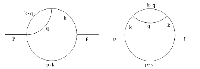
Figure 1: Two-point two-loop Feynman diagrams: Fying-saucer side-view and front-view.

where $\sigma=i+j+l+m+D$.

At this point, our new proposal is to cut the diagram, solve each part separately and then “glue” them together. We expect, of course, that the final result should be the same as in (7). In Fig. 2, we show the two manners to cut this diagram. The first way leaves a one-loop sword-fish graph plus a vertex, whereas the second way leaves a one-loop triangle and a propagator. In the next sections, we solve them in details.

3 The sword-fish diagram

We begin with the generating integral (4), where one can integrate first in the $q$ momentum,

$$I(p^{2};D)=\int d^{D}k\exp[-\beta k^{2}-\gamma(p-k)^{2}]\int d^{D}q\exp[-\alpha q^{2}-\omega(k-q)^{2}]\text{,}$$ (8)

which represents a one-loop with two massless propagators. Completing the square, the $q$ integral can be solved easily, giving

$$I_{q}(k^{2};D)=\left(\frac{\pi}{\alpha+\omega}\right)^{\frac{D}{2}}\exp\left[-\frac{\alpha\omega k^{2}}{\alpha+\omega}\right]\text{.}$$ (9)

Expanding this result in Taylor series and using the multinomial expansion, one obtains

$$I_{q}(k^{2};D)=(\pi)^{\frac{D}{2}}\overset{\infty}{\underset{n_{i}=0}{\sum}}\frac{(-k^{2})^{n_{1}}(-n_{1}-\frac{1}{2}D)!\alpha^{n_{1}+n_{2}}\omega^{n_{1}+n_{3}}}{n_{1}!n_{2}!n_{3}!}\text{,}$$ (10)

with the constraint $-n_{1}-\frac{1}{2}D=n_{2}+n_{3}$ coming from the multinomial expansion.

The next step is to also expand the $q$ gaussian integral (8) in Taylor series,

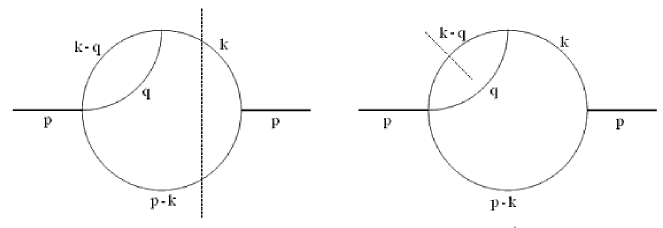
Figure 2: Two-point two-loop Feynman diagrams solved using a ”gluing” technique. We show two ways of cutting them in order to integrate loop-by-loop.

$$I_{q}(k^{2};D)=\overset{\infty}{\underset{i,j=0}{\sum}}(-1)^{i+j}\frac{\alpha^{i}\omega^{m}}{i!m!}\Im_{q}(i,m;D;k^{2})\text{,}$$ (11)

where

$$\Im_{q}(i,m;D;k^{2})=\int d^{D}q(q^{2})^{i}[(k-q)^{2}]^{m}\text{.}$$ (12)

This is the main sword-fish integral in negative dimension. The exponents of the propagators are positive and one has to consider a negative $D$. In the end of the calculation, one does an analytic continuation of the result to negative exponents and positive $D$. Comparing (10) and (11), an expression for the negative-$D$ integral can be written,

$$\Im_{q}(i,m;D;k^{2})=(-\pi)^{\frac{D}{2}}\overset{\infty}{\underset{n_{i}=0}{\sum}}\frac{(k^{2})^{n_{1}}G}{n_{1}!n_{2}!n_{3}!}\delta_{i,n_{1}+n_{2}}\delta_{m,n_{1}+n_{3}}\text{,}$$ (13)

where a product of gamma functions is defined,

$$G=\Gamma(1+i)\Gamma(1+m)\Gamma(1+i+m-2n_{1})\text{.}$$ (14)

The Kronecker’s deltas in (13) and the constraint of the multinomial expansion of (10) form a system of three equations and three unknowns,

$$\left\{\begin{array}[c]{l}n_{1}+n_{2}=i\\ n_{1}+n_{3}=m\\ n_{1}+n_{2}+n_{3}=-\frac{1}{2}D\end{array}\right.$$ (15)

that can be easily solved with a unique solution. The integral $\Im_{q}(i,m;D;k^{2})$ is then given by

$$\Im_{q}(i,m;D;k^{2})=(-\pi)^{\frac{D}{2}}(k^{2})^{i+m+\frac{1}{2}D}P(i,m;D)\text{,}$$ (16)

where

$$P(i,m;D)=\frac{\Gamma(1+i)\Gamma(1+m)\Gamma(1-i-m-D)}{\Gamma(1+i+m+\frac{1}{2}D)\Gamma(1-i-\frac{1}{2}D)\Gamma(1-m-\frac{1}{2}D)}\text{.}$$ (17)

With this result, it is straightforward to find the solution of the complete flying saucer diagram. From the Taylor series (6), it can be seen that the integral in $q$ is already done, so putting (16) in (6), one has

$$\Im(i,j,l,m;D;p^{2})=(-\pi)^{\frac{D}{2}}P(i,m;D)\int d^{D}k(k^{2})^{j+i+m+\frac{1}{2}D}[(p-k)^{2}]^{l}\text{,}$$ (18)

but this is exactly the integral (12) with the variables $\Im_{k}(i+j+m+\frac{1}{2}D,l;D;p^{2})$, that is,

$$\Im(i,j,l,m;D;p^{2}) =(-\pi)^{D}(p^{2})^{i+j+l+m+D}P(i,m;D)$$

$$\times P(i+j+m+\frac{1}{2}D,l;D)\text{,}$$ (19)

and, finally,

$$\left.\Im(i,j,l,m;D;p^{2})=(-\pi)(p^{2})^{\sigma}\frac{\Gamma(1+i)\Gamma(1+l)\Gamma(1+m)}{\Gamma(1+\sigma)\Gamma(1-i-\frac{1}{2}D)\Gamma(1-m-\frac{1}{2}D)}\right.$$

$$\left.\times\frac{\Gamma(1-\sigma-\frac{1}{2}D)\Gamma(1+i+j+m+\frac{1}{2}D)\Gamma(1-i-m-D)}{\Gamma(1-l-\frac{1}{2}D)\Gamma(1+i+m+\frac{1}{2}D)\Gamma(1+l-\sigma)}\right.\text{,}$$ (20)

which is exactly (7), with $\sigma=i+j+l+m+D$. This procedure to solve the flying saucer diagram is much simpler and faster than solving the complete diagram as it was done in [19].

4 The off-shell one-loop triangle diagram

In this section we present the other mode of cutting the complete diagram. This is by far the most difficult and laborious way; however considering the importance of the triangle diagram and the new result that we will show justify the whole process. Instead of (8), one could begin with the $k$ integral:

$$I(p^{2};D)=\int d^{D}q\exp[-\alpha q^{2}]\int d^{D}k\exp[-\beta k^{2}-\gamma(p-k)^{2}-\omega(k-q)^{2}]\text{,}$$ (21)

that corresponds to a one-loop three point function. Working on the $k$ integral, it gives without trouble,

$$I_{k}(p^{2},q^{2};D)=\left(\frac{\pi}{\beta+\gamma+\omega}\right)^{\frac{D}{2}}\exp\left[-\frac{\beta\gamma p^{2}+\beta\omega q^{2}+\gamma\omega r^{2}}{\beta+\gamma+\omega}\right]\text{,}$$ (22)

with $r=q-p$. Expanding (22) in Taylor series, one gets

$$\left.I_{k}(p^{2},q^{2};D)=\left(\pi\right)^{\frac{D}{2}}\underset{n_{i}=0}{\overset{\infty}{\sum}}\frac{(-1)^{n_{1}+n_{2}+n_{3}}(-n_{1}-n_{2}-n_{3}-\frac{1}{2}D)!}{n_{1}!n_{2}!n_{3}!n_{4}!n_{5}!n_{6}!}\right.$$

$$\left.\times(p^{2})^{n_{1}}(q^{2})^{n_{2}}(r^{2})^{n_{3}}\beta^{n_{1}+n_{2}+n_{4}}\gamma^{n_{1}+n_{3}+n_{5}}\omega^{n_{2}+n_{3}+n_{6}}\right.\text{,}$$ (23)

with the constraint $n_{1}+n_{2}+n_{3}+n_{4}+n_{5}+n_{6}=-\frac{1}{2}D$ coming from the multinomial expansion. Now one expands the original $k$ integral (21) in Taylor series, obtaining

$$I_{k}(p^{2},q^{2};D)=\underset{j,l,m=0}{\overset{\infty}{\sum}}\frac{(-1)^{j+l+m}}{j!l!m!}\beta^{j}\gamma^{l}\omega^{m}\Im_{k}(j,l,m;D;p^{2},q^{2})\text{,}$$ (24)

where the corresponding integral in NDIM is

$$\Im_{k}(j,l,m;D;p^{2},q^{2})=\int d^{D}k(k^{2})^{j}[(p-k)^{2}]^{l}[(k-q)^{2}]^{m}\text{.}$$ (25)

Comparing (23) and (24) by its $\beta$, $\gamma$ and $\omega$ powers, the integral $\Im_{k}$ has a general relation,

$$\left.\Im_{k}(j,l,m;D;p^{2},q^{2})=(\pi)^{\frac{D}{2}}(-1)^{-j-l-m}\overset{\infty}{\underset{n_{i}=0}{\sum}}\left[\frac{(-1)^{n_{1}+n_{2}+n_{3}}G}{n_{1}!n_{2}!n_{3}!n_{4}!n_{5}!n_{6}!}\right.\right.$$

$$\left.\times(p^{2})^{n_{1}}(q^{2})^{n_{2}}(r^{2})^{n_{3}}\delta_{j,n_{1}+n_{2}+n_{4}}\delta_{l,n_{1}+n_{3}+n_{5}}\delta_{m,n_{2}+n_{3}+n_{6}}\right]\text{,}$$ (26)

where

$$G=\Gamma(1+j)\Gamma(1+l)\Gamma(1+m)\Gamma(1-n_{1}-n_{2}-n_{3}-\frac{1}{2}D)\text{.}$$ (27)

Considering the deltas in (26) and the multinomial expansion in (23), all the constraints of the problem are

$$\left\{\begin{array}[c]{l}n_{1}+n_{2}+n_{4}=j\\ n_{1}+n_{3}+n_{5}=l\\ n_{2}+n_{3}+n_{6}=m\\ n_{1}+n_{2}+n_{3}=\phi\end{array}\right.\text{,}$$ (28)

where $\phi=j+l+m+\frac{1}{2}D$.

Therefore one has a system of four equations and six variables. There are C${}_{2}^{6}=15$ possible ways to solve the system leaving two free variables, that is, ending up with a double series. From these $15$ possibilities, $3$ have zero determinant, so there are only $12$ non-trivial solutions that can be grouped together according to the ratio of the momenta, or in other words, according to the kinematical configuration. Usually, the groups are made by four solutions and each one is linked to the others considering the symmetries of the diagram. As said before, the leftover variables of the sum form a double series that can be written in terms of Appel hypergeometric functions $F_{4}$ [23],

$$F_{4}\left(a,b,c,d;x,y\right)=\underset{m,n=0}{\overset{\infty}{\sum}}\frac{(a)_{m+n}(b)_{m+n}}{(c)_{m}(d)_{n}}\frac{x^{m}y^{n}}{m!n!}\text{,}$$ (29)

with the Pochhammer symbol designated by

$$(a|m)\equiv(a)_{m}=\frac{\Gamma(a+m)}{\Gamma(a)}\text{,}$$ (30)

and obeying the useful relations

$$(a|m+n) =(a|m)(a+m|n)$$

$$(a|-m) =\frac{\left(-1\right)^{m}}{\left(1-a\mid m\right)}\text{.}$$ (31)

In terms of these definitions, the first set of solutions is

$$\left.\Im_{k}^{1}(j,l,m;D;p^{2},q^{2})=(-\pi)^{\frac{D}{2}}\right.$$

$$\left.\times\left[A_{1}F_{4}\left(-j,-\phi,1+l-\phi,1+m-\phi;\frac{q^{2}}{r^{2}},\frac{p^{2}}{r^{2}}\right)\right.\right.$$

$$\left.+A_{2}F_{4}\left(-l,-j-l+\phi,1-l+\phi,1+m-\phi;\frac{q^{2}}{r^{2}},\frac{p^{2}}{r^{2}}\right)\right.$$

$$\left.+A_{3}F_{4}\left(-m,-j-m+\phi,1+l-\phi,1-m+\phi;\frac{q^{2}}{r^{2}},\frac{p^{2}}{r^{2}}\right)\right.$$

$$\left.\left.+A_{4}F_{4}\left(-l-m+\phi,\phi+\frac{1}{2}D,1-l+\phi,1-m+\phi;\frac{q^{2}}{r^{2}},\frac{p^{2}}{r^{2}}\right)\right.\right]\text{,}$$ (32)

where the multiplicative factors are

$$\begin{array}[c]{l}A_{1}=\left(r^{2}\right)^{\phi}\frac{\left(1+\phi\mid-2\phi-\frac{1}{2}D\right)}{\left(1+l\mid-\phi\right)\left(1+m\mid-\phi\right)}\\ \\ A_{2}=\left(q^{2}\right)^{\phi}\left(\frac{q^{2}}{r^{2}}\right)^{-l}\frac{\left(1+\phi-l\mid-2\phi+l-\frac{1}{2}D\right)}{\left(1+j\mid l-\phi\right)\left(1+m\mid-\phi\right)}\\ \\ A_{3}=\left(p^{2}\right)^{\phi}\left(\frac{p^{2}}{r^{2}}\right)^{-m}\frac{\left(1+\phi-m\mid-2\phi+m-\frac{1}{2}D\right)}{\left(1+j\mid m-\phi\right)\left(1+l\mid-\phi\right)}\\ \\ A_{4}=\left(\frac{p^{2}q^{2}}{r^{2}}\right)^{\phi}\left(\frac{p^{2}}{r^{2}}\right)^{-m}\left(\frac{q^{2}}{r^{2}}\right)^{-l}\frac{\left(1-j-\frac{1}{2}D\mid 2j+\frac{1}{2}D\right)}{\left(1+l\mid j+\frac{1}{2}D\right)\left(1+m\mid j+\frac{1}{2}D\right)}\end{array}$$ (33)

This result agrees with the one calculated in the first reference in [4]. The other two sets with the remaining eight solutions can be found making the replacements

$$\begin{array}[c]{l}\Im_{k}^{2}(j,l,m;D;p^{2},q^{2})=\Im_{k}^{1}(q\leftrightarrow r,j\leftrightarrow l)\\ \Im_{k}^{3}(j,l,m;D;p^{2},q^{2})=\Im_{k}^{1}(p\leftrightarrow r,j\leftrightarrow m)\end{array}$$ (34)

Now, it comes the crucial new step that will permit us to complete the integral (21). As presented in (32), the solution is not valid in the whole space, nor takes into account the momentum conservation $r=q-p$. This last constraint subtly reduces the number of functions $F_{4}$ from four to three because those original four are not linearly independent as they should be to form a basis. Two of them can be rewritten in terms of another function $F_{4}$ that pertains to one of the other sets of different kinematical regions (34). So, with the constraint of momentum conservation, there are only three linearly independent hypergeometric solutions $F_{4}$ and they hold on the whole space. In order to reduce the four functions $F_{4}$ in the solution (32), we need to combine two of them to give another $F_{4}$ in a different kinematical region. The right way to do this combining is given in [22] considering the analogy between Feynman diagrams and electric circuits. Then, applying this to our case, we need to keep the first and the third terms, and the second and fourth ones are combined together using the relation

$$\left.F_{4}\left(a,b,c,d;x,y\right)=\frac{(b)_{-a}}{(d)_{-a}}(-y)^{-a}F_{4}\left(a,a+1-d,c,a+1-b;\frac{x}{y},\frac{1}{y}\right)+\right.$$

$$\left.+\frac{(a)_{-b}}{(d)_{-b}}(-y)^{-b}F_{4}\left(b+1-d,b,c,b+1-a;\frac{x}{y},\frac{1}{y}\right)\right.$$ (35)

to see that the resulting $F_{4}$ is exactly a function that appears in $\Im_{k}^{3}(j,l,m;D;p^{2},q^{2})$ given in (34). So (32) is in fact given by

$$\left.\Im_{k}^{1}(j,l,m;D;p^{2},q^{2})=(-\pi)^{\frac{D}{2}}\times\right.$$

$$\left.\times\left[A_{1}F_{4}\left(-j,-\phi,1+l-\phi,1+m-\phi;\frac{q^{2}}{r^{2}},\frac{p^{2}}{r^{2}}\right)+\right.\right.$$

$$\left.+A_{3}F_{4}\left(-m,-j-m+\phi,1+l-\phi,1-m+\phi;\frac{q^{2}}{r^{2}},\frac{p^{2}}{r^{2}}\right)+\right.$$

$$\left.\left.+A_{5}F_{4}\left(-l,-m-l+\phi,1+j-\phi,1-l+\phi;\frac{r^{2}}{p^{2}},\frac{q^{2}}{p^{2}}\right)\right.\right]\text{,}$$ (36)

where

$$A_{5}=\left(q^{2}\right)^{\phi}\left(\frac{q^{2}}{p^{2}}\right)^{-l}\frac{\left(1+\phi-l\mid-2\phi+l-\frac{1}{2}D\right)}{\left(1+m\mid l-\phi\right)\left(1+j\mid-\phi\right)}$$

.

The kinematic region of the last term is distinct from the previous ones, but as can be seen in Fig. 3, these two regions are connected, allowing the momentum to hold from $-\infty$ to $+\infty$.

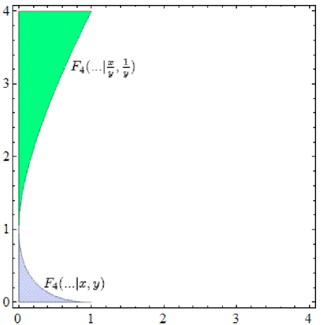
Figure 3: Region of convergence of the hypergeometric series F4 when one does the correct transformation in order to account the momentum constraint.

With the solution (36) in hands, it is now possible to finish the work. Going back to (6), the $k$ integral is done, so putting (36) in it,

$$\Im(i,j,l,m;D;p^{2})=\int d^{D}q(q^{2})^{i}\Im_{k}^{1}(j,l,m;D;p^{2},q^{2})\text{,}$$ (37)

which gives us three integrals of self-energy type, e.g. (12),

$$\left.\Im(i,j,l,m;D;p^{2})=(-\pi)^{\frac{D}{2}}\underset{a,b=0}{\overset{\infty}{\sum}}\int d^{D}q\left\{A_{1}^{{}^{\prime}}(q^{2})^{i+a}\left[\left(q-p\right)^{2}\right]^{\phi-a-b}+\right.\right.$$

$$\left.\left.+A_{3}^{{}^{\prime}}(q^{2})^{i+a}\left[\left(q-p\right)^{2}\right]^{m-a-b}+A_{5}^{{}^{\prime}}(q^{2})^{\phi+i-l+a}\left[\left(q-p\right)^{2}\right]^{b}\right\}\text{,}\right.$$ (38)

where

$$A_{1}^{{}^{\prime}} =\frac{(-j)_{a+b}(-\phi)_{a+b}\left(1+\phi\right)_{-2\phi-\frac{1}{2}D}}{(1+l-\phi)_{a}(1+m-\phi)_{b}\left(1+l\right)_{-\phi}\left(1+m\right)_{-\phi}}\frac{\left(p^{2}\right)^{b}}{a!b!}$$

$$A_{3}^{{}^{\prime}} =\frac{(-m)_{a+b}(-j-m+\phi)_{a+b}\left(1+\phi-m\right)_{-2\phi+m-\frac{1}{2}D}}{(1+l-\phi)_{a}(1-m+\phi)_{b}\left(1+j\right)_{m-\phi}\left(1+l\right)_{-\phi}}\frac{\left(p^{2}\right)}{a!b!}^{\phi+b-m}$$

$$A_{5}^{{}^{\prime}} =\frac{(-l)_{a+b}(-m-l+\phi)_{a+b}\left(1+\phi-l\right)_{-2\phi+l-\frac{1}{2}D}}{(1+j-\phi)_{a}(1-l+\phi)_{b}\left(1+m\right)_{l-\phi}\left(1+j\right)_{-\phi}}\frac{\left(p^{2}\right)^{l-a-b}}{a!b!}$$ (39)

Using the solution (16) with the right replacements of the variables, one gets

$$\Im(i,j,l,m;D;p^{2})=I_{1}+I_{3}+I_{5}\text{,}$$ (40)

where

$$\left.I_{1}=(-\pi)^{D}\left(p^{2}\right)^{i+\phi+\frac{1}{2}D}\frac{\left(1+\phi\right)_{-2\phi-\frac{1}{2}D}}{\left(1+l\right)_{-\phi}\left(1+m\right)_{-\phi}}\right.$$

$$\left.\times\frac{\Gamma(1+i)\Gamma(1+\phi)\Gamma(1-i-\phi-D)}{\Gamma(1+i+\phi+\frac{1}{2}D)\Gamma(1-i-\frac{1}{2}D)\Gamma(1-\phi-\frac{1}{2}D)}\right.$$

$$\left.\times\overset{\infty}{\underset{a,b=0}{\sum}}\frac{(-j)_{a+b}(1+i)_{a}(i+\frac{1}{2}D)_{a}(1-i-\phi-D)_{b}(-i-\phi-\frac{1}{2}D)_{b}}{a!b!(1+l-\phi)_{a}(1+m-\phi)_{b}(1-\phi-\frac{1}{2}D)_{a+b}}\right.$$ (41)

$$\left.I_{3}=(-\pi)^{D}\left(p^{2}\right)^{i+\phi+\frac{1}{2}D}(-1)^{m}\frac{\left(1+\phi\right)_{-2\phi-\frac{1}{2}D}(-\phi)_{m}}{\left(1+j\right)_{-\phi}\left(1+l\right)_{-\phi}\left(1+j-\phi\right)_{m}}\right.$$

$$\left.\times\frac{\Gamma(1+i)\Gamma(1+m)\Gamma(1-i-m-D)}{\Gamma(1+i+m+\frac{1}{2}D)\Gamma(1-i-\frac{1}{2}D)\Gamma(1-m-\frac{1}{2}D)}\overset{\infty}{\underset{a,b=0}{\sum}}\left[\frac{(1+i)_{a}}{a!b!}\right.\right.$$

$$\left.\left.\times\frac{(1-i-m-D)_{b}(i+\frac{1}{2}D)_{a}(-i-m-\frac{1}{2}D)_{b}(-j-m+\phi)_{a+b}}{(1+l-\phi)_{a}(1-m+\phi)_{b}(1-m-\frac{1}{2}D)_{a+b}}\right]\right.$$ (42)

$$\left.I_{5}=(-\pi)^{D}\left(p^{2}\right)^{i+\phi+\frac{1}{2}D}(-1)^{l}\frac{\left(1+\phi\right)_{-2\phi-\frac{1}{2}D}(-\phi)_{l}}{\left(1+j\right)_{-\phi}\left(1+m\right)_{-\phi}\left(1+m-\phi\right)_{l}}\times\right.$$

$$\left.\times\frac{\Gamma(1)\Gamma(1+i-l+\phi)}{\Gamma(1+i-l+\phi+\frac{1}{2}D)\Gamma(1-\frac{1}{2}D)}\overset{\infty}{\underset{a,b=0}{\sum}}\left[\frac{(1)_{b}(1+i-l+\phi)_{a}}{a!b!(1+i-l+\phi+\frac{1}{2}D)_{a+b}}\times\right.\right.$$

$$\left.\left.\times\frac{\left(i-l+\phi+\frac{1}{2}D\right)_{a}(\frac{1}{2}D)_{b}(-l)_{a+b}(-l-m-\phi)_{a+b}}{(1-l-+)_{a}(1+j-\phi)_{b}(i-l+\phi+D)_{a+b}}\right]\right.\text{.}$$ (43)

The summations above can not be written in terms of a known hypergeometric series with defined properties. So one has to specify the values of the indices $i,j,l,m$ and make the analytic continuation. Using (31), it can be seen that due to the analytic continuation of the terms $\frac{\Gamma(1)}{\Gamma(1-\frac{1}{2}D)}$ in (43), $I_{5}$ vanishes. Making $i=-1$ in $I_{1}$ and $I_{3}$, the terms $(1+i)_{a}=\frac{\Gamma\left(a\right)}{\Gamma\left(0\right)}$ cancel the sum in the index $a$ and one has

$$\left.I_{1}=(-\pi)^{D}\left(p^{2}\right)^{i+\phi+\frac{1}{2}D}\frac{\left(1+\phi\right)_{-2\phi-\frac{1}{2}D}}{\left(1+l\right)_{-\phi}\left(1+m\right)_{-\phi}}\right.$$

$$\left.\times\frac{\Gamma(1+i)\Gamma(1+\phi)\Gamma(1-i-\phi-D)}{\Gamma(1+i+\phi+\frac{1}{2}D)\Gamma(1-i-\frac{1}{2}D)\Gamma(1-\phi-\frac{1}{2}D)}\right.$$

$$\left.\times\text{ }_{2}F_{1}\left(-j,1-i-\phi-D,1+m-\phi;1\right)\right.\text{,}$$ (44)

$$\left.I_{3}=(-\pi)^{D}\left(p^{2}\right)^{i+\phi+\frac{1}{2}D}(-1)^{m}\frac{\left(1+\phi\right)_{-2\phi-\frac{1}{2}D}(-\phi)_{m}}{\left(1+j\right)_{-\phi}\left(1+l\right)_{-\phi}\left(1+j-\phi\right)_{m}}\right.$$

$$\left.\times\frac{\Gamma(1+i)\Gamma(1+m)\Gamma(1-i-m-D)}{\Gamma(1+i+m+\frac{1}{2}D)\Gamma(1-i-\frac{1}{2}D)\Gamma(1-m-\frac{1}{2}D)}\right.$$

$$\left.\times\text{ }_{2}F_{1}\left(1-i-m-D,-j-m+\phi,1-m+\phi;1\right)\right.\text{,}$$ (45)

where

$${}_{2}F_{1}\left(a,b,c;x\right)=\underset{m=0}{\overset{\infty}{\sum}}\frac{(a)_{m}(b)_{m}}{(c)_{m}}\frac{x^{m}}{m!}$$ (46)

is a hypergeometric series that can be summed up when it has unit argument,

$${}_{2}F_{1}\left(a,b,c;1\right)=\frac{\Gamma\left(c\right)\Gamma\left(c-a-b\right)}{\Gamma\left(c-a\right)\Gamma\left(c-b\right)}\text{.}$$ (47)

Using the property (47) in (44, 45), making the analytic continuation and specifying $i=j=l=m=-1$, the integral (40) becomes

$$\left.\Im_{AC}(i,j,l,m;D;p^{2})=(\pi)^{D}\left(p^{2}\right)^{D-4}\frac{\Gamma^{3}\left(\frac{1}{2}D-1\right)\Gamma\left(D-3\right)}{\Gamma\left(3-\frac{1}{2}D\right)\Gamma\left(D-2\right)}\times\right.$$

$$\left.\times\frac{\Gamma\left(2-\frac{1}{2}D\right)\Gamma\left(4-D\right)}{\Gamma\left(\frac{3}{2}D-4\right)}\right.\text{,}$$ (48)

which gives the exact result of the flying saucer diagram if one makes the analytic continuation and the specification of the exponents in the solution (7).

5 Conclusion

We presented in this work a technique to integrate multi-loop Feynman integrals. In our approach one can carry out the integrals loop-by-loop using well-known results of straightforward one-loop diagrams. We point out the advantage that each diagram when properly calculated — with off-shell external legs and respecting the constraint on the external momenta — can be used to solve an even harder diagram and so forth. In this approach each diagram can be considered as a building block of another one, with more legs and/or loops. The same method can also be applied to the two-loop master integral and a result valid for arbitrary exponents of propagators can be obtained.

Acknowledgments

J. D. Bolzan wishes to thank CNPq (Conselho Nacional de Desenvolvimento Científico e Tecnológico) for financial support. AGMS gratefully acknowledges Brazilian agencies CNPq (projects 312000/2006-5 and 471018/2007-4) and FAPERJ (projects E26/171.191-2007 and E26/170.374-2007).

References

• [1] T. Kinoshita, T. Aoyama, M. Hayakawa , M. Nio, Nucl.Phys. B (Proc. Suppl.) 160 (2006) 235. T. Kinoshita, Nucl.Phys. B (Proc. Suppl.) 157 (2006) 101.
• [2] G. ’t Hooft, M. Veltman, Nucl. Phys. B44 (1972) 189. C.G. Bollini, J.J. Giambiagi, Nuovo Cimento B12 (1972) 20. J.F.Ashmore, Comm. Math. Phys. 29 (1973) 177.
• [3] G. M. Cicuta, E. Montaldi, Lett. Nuovo Cim. 4 (1970) 329.
• [4] A.I. Davydychev, J. Math. Phys. 32 (1991) 1052; A.I. Davydychev, J. Math. Phys. 33 (1991) 358.
• [5] V.A. Smirnov, Nucl. Phys. B566 (200) 469; Phys. Lett. B460 (1999) 397.
• [6] J.B. Tausk, Phys. Lett. B469 (1999) 225.
• [7] K.G. Chetyrkin, A.L. Kataev, F.V. Tkachov, Nucl. Phys. B174 (1980) 345; K.G. Chetyrkin, F.V. Tkachov, Nucl. Phys. B192 (1981) 159.
• [8] T.Gehrmann, E. Remiddi, Nucl.Phys. B580 (2000) 485.
• [9] S. Laporta, P. Mastrolia, E. Remiddi, Nucl. Phys. B 688 (2004) 165.
• [10] I.G. Halliday, R.M. Ricotta, Phys. Lett. B193 (1987) 241. R.M.Ricotta, Topics in Field Theory, (Ph.D. Thesis, Imperial College, 1987). G.V. Dunne, I.G. Halliday, Phys. Lett. B193 (1987) 247.
• [11] C. Anastasiou, E.W.N. Glover, C. Oleari, Nucl. Phys. B572 (200) 307; Nucl. Phys. B565 (2000) 445.
• [12] A.T.Suzuki, E.S.Santos, A.G.M.Schmidt, J.Phys.A36 (2003) 4465.
• [13] A.T. Suzuki, A.G.M. Schmidt, JHEP 09(1997)002 ; Phys. Rev. D58 (1998) 047701; Can.J.Phys.84 (2006) 213.
• [14] I.Gonzalez, I. Schmidt, Nucl. Phys. B769 (2007) 124.
• [15] A.T. Suzuki, A.G.M. Schmidt, J.Phys.A 33 (2000) 3713.
• [16] A.T. Suzuki, A.G.M. Schmidt, Eur. Phys. J. C10 (1999) 357; Eur. Phys. J. C12 (2000) 361.
• [17] C. Anastasiou, L. Dixon, Z. Bern, D.A.Kosower, Phys.Rev. Lett. 91 (2003) 251602; D. Nguyen, M. Spradlin, A.Volovich, Phys.Rev. D77 (2008) 025018; Z.Bern, J.J.M.Carrasco, H.Johansson, D.A.Kosower, Phys.Rev. D76 (2007) 125020; Z.Bern, M.Czakon, D.A.Kosower, R.Roiban, V.A.Smirnov, Phys.Rev. Lett. 97 (2006) 181601.
• [18] É.É.Boos, A.I.Davydychev, Theor.Math.Phys.89 (1991) 1052.
• [19] A.T. Suzuki, A.G.M. Schmidt, Eur. Phys. J. C5 (1998) 175.
• [20] S. Weinzierl, I.Bierenbaum, Eur. Phys. J. C32 (2003) 67.
• [21] V. Kostrykin, R. Schrader, J. Phys. A 32 (1999) 595; Fortschritte der Physik 48 (2000) 703.
• [22] A. T. Suzuki, e-Print: arXiv:0706.1082 [hep-th].
• [23] I.S. Gradshteyn, I.M. Rhizik, Table of integrals, series and products (Academic Press, 1994).