Optimal Markov Approximations and Generalized Embeddings

Abstract

Based on information theory, we present a method to determine an optimal Markov approximation for modelling and prediction from time series data. The method finds a balance between minimal modelling errors by taking as much as possible memory into account and minimal statistical errors by working in embedding spaces of rather small dimension. A key ingredient is an estimate of the statistical error of entropy estimates. The method is illustrated with several examples and the consequences for prediction are evaluated by means of the root mean squard prediction error for point prediction.

I Introduction

Given is a univariate time series $\{x_{i}:i=1,\ldots,N\}$, obtained from the time evolution of some deterministic or stochastic dynamical system by applying a scalar measurement function to the state vectors of this system. We will assume that the measurements are equidistant in time. A meanwhile standard approach to the modelling and prediction based on univariate time series data starts from the construction of a multidimensional state space. Commonly used is the time delay embedding space. In the case of deterministic dynamics, the Takens theorem takens81 states that if the embedding dimension $m$ satisfies $m>2D_{f}$, where $D_{f}$ is the fractal dimension of the attractor, then m-dimensional delay vectors $(x_{n-k(m-1)},x_{n-k(m-2)},\ldots,x_{n})$ with delay $k$ can be uniquely mapped onto the non-observed state vectors. Hence the process in the m-dimensional delay embedding space is deterministic in the sense of the existence and uniqueness of the solution of the initial value problem. In special cases, smaller values of $m$ might be sufficient for reconstruction of the underlying dynamics.

As it has been argued recently paparella97 ; kantzholst04 , also the modelling and prediction of time series data from stochastic processes can profit from the concept of state space reconstruction: In an ideal situation, there exists a time delay embedding space, in which the stochastic dynamics is Markovian of (possibly higher) order $m$, i.e., in which the conditional probability density function (pdf) $\rho(x_{n}|x_{n-m},\ldots,x_{n-1})$ to find a given future value cannot be made narrower by including more past values into the condition. In the framework of time series analysis, the conditional pdf has to be estimated from the data. This can be done by either estimating conditional probabilities through binning and counting kantzholst04 , or by kernel estimators silverman92 . Two consequences arise: These estimates are subject to statistical errors, and a length scale $\epsilon$ is introduced, i.e., the estimated conditional probabilities do not vary as a function of the condition $(x_{n-m},\ldots,x_{n-1})$ on length scales smaller than $\epsilon$. The statistical error is a function of not only the dataset size $N$ but also of the spatial resolution $\epsilon$. When models have to be fitted to observed data, model parameters are to be determined. The estimated conditional probabilities can be interpreted as the model parameters of a Markov model. In data analysis tasks the Markov order $m$, however, usually is not a priori known, and has to be obtained from the data.

In both the deterministic and the stochastic cases, finding the suitable embedding dimension is one of the practical issues. In the stochastic case the embedding dimension can be associated with the number of time steps of nonvanishing condition, which under absence of intermediate time steps of vanishing condition reduces to the Markov order $m$. Whereas for the deterministic case mathematically rigorous results saueryorkecasdagli91 as well as numerically efficient and reliable algorithms grassproc83a exist, for the stochastic case only statistically demanding tests of the Chapman Kolmogorov equation are currently in use friedrich97 . In both cases, there exists the practical problem that from a theoretical point of view the embedding dimension for the process could be very large. If the amount of data is insufficient in view of statistical robustness of either the algorithms to determine empirically the embedding dimension or of estimates of, e.g., model parameters in a corresponding space, then a high dimensional model is practically irrelevant, even if theoretically justified. Hence, in many situations an effective model and a different embedding dimension might be superior to the model advised by the structure of the underlying dynamics. We will illustrate this statement later and we will convince the reader of its relevance.

When identifying the optimal embeddings, i.e., when looking for the optimal Markov approximations, we have to take into account two types of errors. The first one is a modelling error, which we make if we ignore components in the past of the time series which are relevant for its future. In the deterministic setting, this would mean that we use an embedding dimension which is too small. In the stochastic setting, it means that the Makovianity of in general higher order or the cardinality of time steps of nonvanishing condition is not fully captured by the chosen embedding space. The second error is a statistical error. Regardless of which quantity is estimated from a finite dataset, its value is always subject to a statistical error. In the context of prediction and modeling, the corresponding samples are usually obtained from neighbourhoods of delay vectors. Sample sizes are small and correspondingly statistical errors large, if we work in embedding spaces whose dimension is too large compared to the amount of available data and compared to the diameter of neighbourhoods, i.e., locality of the estimate.

Hence, what we are proposing here with the intention of a rather general applicability is a concept to identify optimal resolution-dependent Markov approximations, in which the combined effect of modeling errors and statistical errors is minimal.

Practically, we will relate the modelling error to the discrepancy of conditional entropies from entropies with sufficient conditioning. The statistical error of a model will be related to the statistical error in entropy estimation. Therefore, we will carry out explicitly error estimates for entropy estimations. On the route of searching for models which capture the memory of a process but involve an as small as possible embedding dimension, we will consider also non-standard so-called perforated embeddings, namely those, where the temporal spacings between successive elements of a delay vector are not identical for all pairs of adjacent components. Such embeddings were also discussed in garcia05 and pecora06 . This paper makes a new suggestion how to find optimal ones.

In the next section the basic quantities of information theory are introduced, which in the development of the criteria for optimal Markov approximations play a certain role. In Sec.III we remind a widely used procedure for the estimation of entropies and discuss the statistical errors in numerical estimation of the correlation entropy. In Sec.IV a novel method for the selection of usual Markov approximations is presented, but it is immediately pointed out that the framework has to be generalized in order to be suitable for arbitrary dynamics. A unified notation for entropies in the time series analytical framework suitable for the treatment of variable future lead times, jointly conditioned joint entropies, noncausal conditionings, downsampling and arbitrary omissions in conditionings is introduced in Sec.V, which remedies the formerly mentioned problems. The notion of perforatedness is introduced. In Sec.VI we present the method to identify optimal generalized Markov approximations as a function of the data accuracy $\epsilon$ for a given time series of fixed length $N$. Subsequently, the success of the introduced criterion for the determination of optimal perforated Markov approximations is illustrated for several model processes with memory in Sec.VII. We show that indeed the theoretically optimal embedding of the process from the dynamical law behind the generated data sets is not necessarily the optimal state space representation of a finite time series for all resolutions. Furthermore the dependence on the length of the underlying dataset is discussed in detail. Some consequences for prediction with the example of the generalized Henon map are outlined in Sec.VIII. In Sec.IX the results of this paper are concluded.

II Relevant quantities of information theory

The resolution($\epsilon$)-dependent joint Renyi block entropy of order $q$ is given by

$$H_{m}^{(q)}(\epsilon)=\frac{1}{1-q}\ln\left[\sum_{l_{1}=1}^{L_{1}(\epsilon)}\ldots\sum_{l_{m}=1}^{L_{m}(\epsilon)}{(p_{l_{1},\ldots,l_{m}}(\epsilon))}^{q}\right]\;.$$ (1)

It estimates the joint uncertainty of random variables corresponding to $m$ successive time steps of a time series. In case of dependences of random variables a conditional probability distribution is narrower than the corresponding unconditioned probability distribution. Further conditioning into the past in general further decreases the width of the distribution and the uncertainty of the outcome of the random experiment. This behaviour can also be quantified with conditional entropies defined by

$$H_{1|m}(\epsilon):=H_{m+1}(\epsilon)-H_{m}(\epsilon)\;,$$ (2)

as the difference of joint block entropies with different block length. In this formula and the subsequent ones the Renyi order $q$ is notationally omitted. Conditional entropies are interpreted as the remaining uncertainty after having used the information from the chosen conditioning. In case of maximal, i.e. infinite conditioning, the unreducable uncertainty is obtained as

$$H_{1|\infty}(\epsilon)\equiv\lim_{m\rightarrow\infty}H_{1|m}(\epsilon)\;.$$ (3)

The redundancy is defined by

$$R_{m}(\epsilon):=H_{1}(\epsilon)-H_{1|m}(\epsilon)\;,$$ (4)

and hence is interpreted as the uncertainty reduction of the immediate future random variable from conditioning on the adjacent $m$ past time steps. The quantity

$$Q_{m}(\epsilon):=H_{1|m}(\epsilon)-H_{1|\infty}(\epsilon)$$ (5)

is called ignored memory. It is the in principle accessible, but renounced uncertainty reduction of the immediate future random variable. From combining Eq.(4) and Eq.(5) it is possible to see that the total uncertainty of a single random variable is decomposable according to

$$H_{1}(\epsilon)=H_{1|\infty}(\epsilon)+R_{m}(\epsilon)+Q_{m}(\epsilon)\;.$$ (6)

III Estimation of entropic quantities and statistical errors of correlation entropies

Our method for finding optimal Markov approximations will find a balance between maximal uncertainty reduction of future values of the time series and minimized statistical errors. To this end, we will discuss here the estimation of entropies from finite time series and in particular the statistical errors involved in this estimation. Because it is the statistically most robust and algorithmically most convenient quantity, we will concentrate here on the order-2 Renyi entropy $H^{(q=2)}=-\ln\sum p_{i}^{2}$, which is estimated from the Grassberger-Procaccia correlation sum grassproc83a

$$C_{m}^{(2)}(N,\epsilon)=\frac{1}{N(N-1)}\sum_{i=1}^{N}\sum_{k\neq i}\Theta(\epsilon-\|\mathbf{x}_{i}-\mathbf{x}_{k}\|)$$ (7)

by

$$H_{m}^{(2)}(N,\epsilon)=-\ln C_{m}^{(2)}(N,\epsilon)\;.$$ (8)

We use the maximum norm in the argument of the Heaviside function $\Theta$. The conditional entropy of Eq.(2), our construction element for ignored memory and redundancy, is obtained from

$$H_{1|m}^{(2)}(N,\epsilon)=\ln C_{m}^{(2)}(N,\epsilon)-\ln C_{m+1}^{(2)}(N,\epsilon)\;.$$ (9)

As it was shown by Grassberger grassberger03 , the correlation sum does not suffer from systematic finite sample effects, i.e., it is an unbiased estimator of the correlation integral. Consequently, the mean value of estimated quantities such as the correlation entropy or the correlation dimension on data sets of fixed size $N$ for arbitrarily small $\epsilon$ will be correct, as long as the combination $(N,\epsilon)$ is such that the correlation sum is non-zero. However, each individual result is subject to statistical errors. In the following we want to estimate the magnitude of these errors.

To begin with, it is introduced the random variable $W_{m}(\epsilon,\mathbf{x}_{i})$ for the number of similar vectors $\mathbf{x}_{k}$ of $\mathbf{x}_{i}$ with distance smaller than $\epsilon$ according to the chosen norm, i.e., the random variable for the cardinality of the set $\{\mathbf{x}_{k}\in{\mathcal{U}}(\epsilon,\mathbf{x}_{i}):k\in\{1,\ldots,N-m\}\}$, where the $\epsilon$-neighborhood of the vector $\mathbf{x}$ is defined by

$${\mathcal{U}}(\epsilon,\mathbf{x}):=\{\mathbf{z}:\|\mathbf{z}-\mathbf{x}\|<\epsilon\}\;.$$ (10)

$W_{m}(\epsilon,\mathbf{x}_{i})$ is distributed according to a Binomial distribution. For a given dataset, the realization of $W_{m}(\epsilon,\mathbf{x}_{i})$ is given by

$$w_{m}(N,\epsilon,\mathbf{x}_{i}):=\sum_{k=1;k\neq i}^{N}\Theta(\epsilon-\|\mathbf{x}_{i}-\mathbf{x}_{k}\|)\;.$$ (11)

With this expression the correlation sum (Eq.(7)) can be written as

$$C_{m}^{(2)}(N,\epsilon)=\frac{1}{N(N-1)}\sum_{i}w_{m}(N,\epsilon,\mathbf{x}_{i})\;.$$ (12)

Except for very large $\epsilon$ or extremely small $N$ the distribution of the random variable $W_{m}(\epsilon,\mathbf{x}_{i})$ can be excellently approximated by a Poisson distribution. This leads to the property

$$\operatorname{Var}(W_{m}(\epsilon,\mathbf{x}_{i}))=E(W_{m}(\epsilon,\mathbf{x}_{i}))\;,$$ (13)

and therefore

$$\Delta w_{m}(N,\epsilon,\mathbf{x}_{i})\approx\sqrt{w_{m}(N,\epsilon,\mathbf{x}_{i})}\;.$$ (14)

Assuming mutual independence of $W_{m}(\epsilon,\mathbf{x}_{i})$ and using the standard rules for error propagation (additivity of the variances) as well as the approximate relation (14), the statistical error of the correlation sum is estimated by

$$\Delta C_{m}^{(2)}(N,\epsilon) =\frac{1}{N(N-1)}\sqrt{\sum_{i}(\Delta w_{m}(N,\epsilon,\mathbf{x}_{i}))^{2}}$$

$$\approx\frac{1}{N(N-1)}\sqrt{\sum_{i}w_{m}(N,\epsilon,\mathbf{x}_{i})}\;.$$ (15)

Thus it can be computed by using the non-normalized correlation sums, which are needed anyway to estimate entropies. From Eqs.(8), (12) and (III) the statistical error of the Renyi entropy can be calculated as

$$\Delta H_{m}^{(2)}(N,\epsilon)=\frac{\Delta C_{m}^{(2)}(N,\epsilon)}{C_{m}^{(2)}(N,\epsilon)}\approx\frac{1}{\sqrt{\sum_{i}w_{m}(N,\epsilon,\mathbf{x}_{i})}}\;,$$ (16)

and the statistical error of the usual conditional entropy is obtained from

$$\Delta H_{1|m}^{(2)}(N,\epsilon) =\sqrt{[\Delta H^{(2)}_{m+1}(N,\epsilon)]^{2}+[\Delta H^{(2)}_{m}(N,\epsilon)]^{2}}$$

$$\approx\sqrt{\frac{1}{\sum_{i}w_{m+1}(N,\epsilon,\mathbf{y}_{i})}+\frac{1}{\sum_{i}w_{m}(N,\epsilon,\mathbf{x}_{i})}}\;.$$ (17)

Further error propagation for the estimated redundancy

$$\Delta R_{m}\!(N,\epsilon)$$

$$\!=\!\sqrt{[\Delta\!H_{1}\!(N,\epsilon)]^{2}\!\!+\![\Delta\!H_{m+1}\!(N,\epsilon)]^{2}\!\!+\![\Delta\!H_{m}\!(N,\epsilon)]^{2}}$$ (18)

is possible in the same way. This quantity will be needed for the criterion given in Eq.(19).

The assumptions entering the arguments for usual error propagation are:

1. Independence of the random variables

2. Gaussian error statistics

3. Errors are small so that nonlinear expressions can be approximated by first order Taylor expansions around the mean.

The authors are aware of the fact that item 1 is violated, since if $\|\mathbf{x}_{i}-\mathbf{x}_{i^{\prime}}\|<\epsilon$, then the phase space points have overlapping neighborhoods and $W_{m}(\epsilon,\mathbf{x}_{i})$ and $W_{m}(\epsilon,\mathbf{x}_{i^{\prime}})$ are not independent of each other. Correlations among the $W_{m}(\epsilon,\mathbf{x}_{i})$ yield a smaller effective sample size, such that Eq.(16) is an underestimation of the true statistical error of entropies. The violation of the assumption of item 1, however, becomes the less relevant the smaller $\epsilon$, since then the overlap of neighborhoods decreases. Item 2 is violated, since the error statistics of our basic random variables $W_{m}(\epsilon,\mathbf{x}_{i})$ is explicitly non-Gaussian. This violation becomes the stronger the smaller the values of $w_{m}(N,\epsilon,\mathbf{x}_{i})$ become, i.e., for small $\epsilon$. Nevertheless, in spite of those arguments, usual error propagation is used as an approximation of the true errors of the estimation of entropic quantities.

Except for Eq.(22) in the following the dependence on the length $N$ of the dataset will only be shown for the statistical errors, since for the expectation value of entropies and derived quantities there is no dependence on $N$.

IV A novel criterion for usual Markov approximations

As already mentioned in the introduction, there are two kinds of errors involved in our strategy for the determination of optimal Markov approximations:

First, there is a modelling error. If a Markov approximation is carried out, typically information about the future is truncated, which is not anymore available for uncertainty reduction. This renounced uncertainty reduction can be quantified by the ignored memory $Q_{m}$ given in Eq.(5). The value of $Q_{m}$ should be small. It is the smaller (or remains the same) the more components in the past are taken into account, i.e., the higher the order $m$ of the Markov approximation. Naively, one could be tempted to demand that the ignored memory in optimal Markov approximations should vanish, but in case of infinite range of memory in the past the resulting Markov order would be infinite, what cannot be desired with respect to practical applications.

Second, a statistical error has to be discussed. There is an unavoidable statistical error in the estimation of entropies, which is propagated to a nonvanishing statistical error of the performed uncertainty reduction from conditioning. This statistical error quantified by $\Delta R_{m}$ given in Eq.(III) describes the unreproducibility of uncertainty reduction. Also this term should be rather small in order to make the uncertainty reduction confident. $\Delta R_{m}$ increases with larger Markov order $m$, because less neighbors are found in the estimation of the correlation sum under the more restrictive conditions. Demanding only the minimization of the statistical error of the redundancy in a criterion for optimal Markov approximations would thus lead to empty conditionings. It is intuitively clear that also this can in general not be a reasonable solution.

Since in contrast to $Q_{m}$ the term $\Delta R_{m}$ is the smaller the fewer past components are taken into account, the reduction of both errors are complementary demands and one faces an optimzation problem. The aim is now to give a criterion such that for arbitrary dynamics a resolution-dependent optimal Markov approximation can be found. The ad hoc choice for such a criterion reads:

$$m_{\operatorname{opt}}(\epsilon)=\max\{m\in{\mathbb{N}}_{0}:\Delta R_{m}(N,\epsilon)<Q_{m}(\epsilon)\}\;.$$ (19)

The reason for the criterion can be understood from the following: The maximal memory, which in a senseful way to take into account is restricted by the condition that the statistical error of redundancy, i.e., the statistical error of the uncertainty reduction has to be smaller than the ignored memory. Otherwise the ignored memory is anyway not anymore resolvable by enlargement of the order of the Markov approximation. It is used that the statistical error of the redundancy increases with the Markov order, whereas the ignored memory decreases with the Markov order. Hence starting from the smallest possible Markov order $m$ it is increased as long as the statistical error of the redundancy remains smaller than the ignored memory.

The whole reasoning is resolution-dependent. In the Markov model conditional probabilities

$$p_{l_{n}|l_{n-m},\ldots,l_{n-1}}(\epsilon)$$

$$\quad=\negthickspace\int\limits_{B_{l_{n-m},\ldots,l_{n}}(\epsilon)}\negthickspace\negthickspace\negthickspace\negthickspace\negthickspace\negthickspace\negthickspace\negthickspace\rho(x_{n}|x_{n-m},\ldots,x_{n-1})\;dx_{n-m}\ldots dx_{n}\;,$$ (20)

that a state inside some $\epsilon$-subset of the state space is mapped onto some $\epsilon$-interval corresponding to the future, are treated. $B_{l_{n-m},\ldots,l_{n}}(\epsilon)$ is a resolution-dependent (m+1)-dimensional box as an element of the partition of the underlying embedding space. The result are approximations to the true conditional probability density, which vary only on spatial scales which are larger than $\epsilon$. E.g., a model obtained for relatively small $\epsilon$ has the potential to represent very fine structures in the state space, but it suffers from poor statistics. Since for larger $\epsilon$ statistics gets better, but only coarser structures are resolved, the optimal Markov order (and later on the optimal perforated model), as well as prediction errors which will be discussed in Sec. VIII, depend on the spatial resolution $\epsilon$.

Eventually we want to make plausible that the criterion Eq.(19) for $m_{\operatorname{opt}}$ derived from information theory really yields the optimal order of the Markov model describing the underlying dynamics. The conditional probabilities of Eq.(IV) corresponding to a Markov model of order $m$ are estimated from a finite dataset. Hence they are subject to statistical errors, which are the larger the larger $m$. Exactly the same statistical errors of conditional probabilities would lead to statistical errors of the redundancy $\Delta R_{m}$, if we defined all information theoretic quantities through Shannon entropies ($q=1$), and they enter indirectly the statistical errors of quantities based on the Renyi-entropy of order $q=2$ through $\Delta w_{m}$ (cmp. Eqs. (14) and (11)). Hence the statistical error of the redundancy is related to uncertainty of the corresponding Markov model. Since furthermore with increasing conditioning the minimization of the ignored memory $Q_{m}$ is in accordance with the minimization of the modelling error of the Markov model the plausibility argument is complete.

As an example the autoregressive (AR) process

$$x_{n+1}=\sum_{i=0}^{p-1}a_{i}x_{n-i}+\xi_{n+1}$$ (21)

of order $p=3$ with parameters $a_{0}=0.2$; $a_{1}=0.3$; $a_{2}=0.4$ is treated, i.e., a memory depth of three time steps is used. As usual $\xi_{n+1}$ is Gaussian white noise with unit variance and zero mean. A dataset of length $N=50000$ is used. The result is shown in Fig.1.

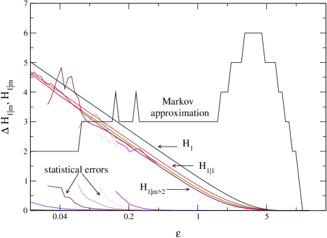
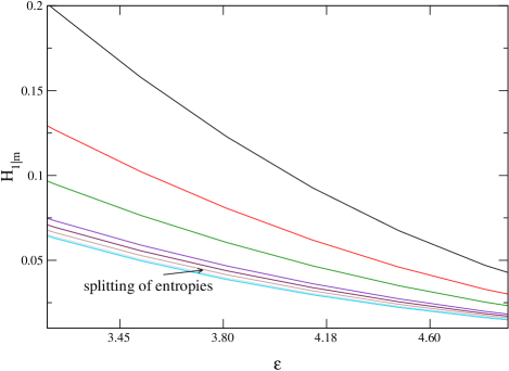
Figure 1: (Color online) Upper panel: Suggestion for resolution-dependent usual Markov approximations for the autoregressive process. Furthermore the conditional entropies $H_{1|m}(\epsilon)$ with varying conditioning as a function of the resolution and the corresponding resolution-dependent statistical error in the estimation of the conditional entropies are shown. Lower panel: Zoom of the upper panel with the intention to make visible the splitting of entropies for rather coarse resolutions, which is detected by the algorithm.

For intermediate resolutions the memory depth $m=p=3$ is exactly found with the algorithm, visible in the upper panel of Fig.1. For higher resolutions, i.e., smaller $\epsilon$, the statistical error dominates the criterion and a truncation for shorter Markov order is enforced. This means that although the data stem from a process of Markov order $p=3$, for the given dataset size and chosen $\epsilon$ an $m=2$ model is superior when estimated from the data. For large $\epsilon$ a suggestion for a larger Markov order can be found. The order of the Markov property given by Eq.(21) is also not preserved under coarse graining, which can be observed by the splitting of entropies with higher conditioning in the lower panel of Fig.1, because for coarser resolutions the mapping onto discrete states becomes noticable and causes extra dependences among the involved random variables shifting information about the future into the further past. Since for coarse resolution the statistical error is extremely small, the splitting of entropies is detected by the criterion as shown in the upper panel of Fig.1.

Whereas the application of the criterion given by Eq.(19) was successful in the previous example, problems do arise in case of more general dynamics. E.g., the discretized Mackey-Glass dynamics to be discussed in Sec.VII.2 leads to a memory structure with omissions, i.e., certain intermediate time steps in the past do not contribute to uncertainty reduction of the future. Under the conditions of this section minimization of the modelling error is in general accompanied by large statistical errors such that true joint minima of both types of errors are not accessed. Hence a more subtle procedure for obtaining optimal Markov approximations should be necessary, in which the minimization of the modelling error by contributions from the further past is not statistically suppressed. A notation for joint entropies on time series segments with omissions has to be introduced. We call such situations ’perforated’, which are worked out in the next section. As we will see, on the other hand, the perforated framework introduces the new problem that with respect to a criterion for an optimal Markov approximation a monotonicity of the relevant entropic quantities in a parameter as the Markov order $m$ in the former case describing all possible conditionings is not anymore available. A solution with a qualitatively slightly different generalized criterion, which nevertheless follows essentially the same idea as in this section, will be offered in Sec.VI.

V Perforation

Whereas in Eq.(1) the uncertainty of $m$ random variables corresponding to successive time steps in a time series is assessed, in this section a notational framework for evaluation of uncertainties of random variables corresponding to arbitrary sets of time steps is introduced. Instead of the number $m$ of successive time steps, which is not anymore enough for characterization of the uncertainty-assessed set of time steps, the relevant set has to be given explicitly. We will denote such sets of integers by ${\bf{J}}$ (or ${\bf{K}}$) and they will be called perforated, if omissions of time steps are involved. E.g., Eq.(8) for the estimation of order-2-Renyi entropies has to be generalized for the perforated case by

$$H_{{\bf{J}}}^{(2)}(N,\epsilon)=-\ln C_{{\bf{J}}}^{(2)}(N,\epsilon)\;,$$ (22)

where the vectors $\mathbf{x}_{i}$, $\mathbf{x}_{k}$ in Eq.(7) for the correlation sum adopt the perforation structure given by ${\bf{J}}$, i.e., if ${\bf{J}}=\{j_{1},j_{2},\ldots,j_{|{\mathbf{J}}|}\}$, then the corresponding generalized delay vector with index $i$ reads $\mathbf{x}_{i}=(x_{i+j_{1}},x_{i+j_{2}},\ldots,x_{i+j_{|{\mathbf{J}}|}})$. This in general leads to non-standard embeddings.

Conditional entropies can be defined in general as

$$H_{{\bf{K}}|{\bf{J}}}^{(2)}(\epsilon):=H_{{\bf{K}}\cup{\bf{J}}}^{(2)}(\epsilon)-H_{{\bf{J}}}^{(2)}(\epsilon)\;.$$ (23)

where ${\bf{K}}$ is a set of integers which is disjoint from ${\bf{J}}$. This quantity in principle allows for the evaluation of entropies with noncausal conditioning. In prediction situations the convention is made that the presence is indicated by the index zero. Hence a set ${\bf{J}}$ of conditioning indices in the past only consists of negative integers $({\bf{J}}\subset\mathbb{Z}_{0}^{-})$, which indicate the respective distances to the presence. With respect to optimal Markov approximations we are interested in single element sets ${\bf{K}}$. In this case the single element denoted by $f$ corresponds to a certain future time step, and Eq.(23) reduces to

$$H_{\{f\}|{\bf{J}}}^{(2)}(\epsilon):=H_{\{f\}\cup{\bf{J}}}^{(2)}(\epsilon)-H_{{\bf{J}}}^{(2)}(\epsilon)\;.$$ (24)

With conditioning on full past for a single time step $f$ in the future the condtional entropy becomes $H_{\{f\}|\mathbb{Z}_{0}^{-}}(\epsilon)$. As a special case of one step ahead the nonperforated conditional entropy with infinite conditioning of Eq.(3) is obtained:

$$H_{\{1\}|\mathbb{Z}_{0}^{-}}(\epsilon)\equiv H_{1|\infty}(\epsilon)\;.$$ (25)

Under perforated circumstances the ignored memory of Eq.(5) is redefined by

$$Q_{\{f\};{\bf{J}}}(\epsilon):=H_{\{f\}|{\bf{J}}}(\epsilon)-H_{\{f\}|\mathbb{Z}_{0}^{-}}(\epsilon)\;,$$ (26)

and the redundancy of Eq.(4) now is obtained from

$$R_{\{f\};{\bf{J}}}(\epsilon):=H_{1}(\epsilon)-H_{\{f\}|{\bf{J}}}(\epsilon)\;.$$ (27)

As a generalization of Eq.(III), the statistical error of the redundancy in Eq.(27), which will be essential for the novel criterion for optimal perforated Markov approximations, still obtained from usual error propagation, reads

$$\Delta R_{\{f\};{\mathbf{J}}}(N,\epsilon)$$

$$\!=\!\sqrt{[\Delta\!H_{1}(N,\epsilon)]^{2}\!\!+\![\Delta\!H_{\{f\}\cup{\bf{J}}}(N,\epsilon)]^{2}\!\!+\![\Delta\!H_{\bf{J}}(N,\epsilon)]^{2}}$$ (28)

After having fixed the notational framework for a perforated treatment, a suitable generalization of the criterion for optimal usual Markov approximations of Sec.IV can be given such that simultaneous minimization of as well the modelling error as also the statistical error makes sense also for generalized dynamics containing inhomogeneously distributed memory in the past. Moreover, the new notation in principle allows for a treatment of variable future time steps, jointly conditioned joint entropies, arbitrary omissions in conditionings, noncausal conditionings and downsampling in a unified framework.

VI A novel criterion for optimal generalized Markov approximations

Also in the perforated case we consider the two types of errors already discussed in the context of usual Markov approximations, i.e., the modelling error and the statistical error, which have to be minimized jointly. As in Sec.IV the two errors are again quantified by the ignored memory, i.e., ignored potentially usable information, and the statistical error of redundancy, however, in this case with usage of variants of those quantities respecting perforatedness as introduced in Sec.V. The minimization of the single errors is again complementary in the number of conditioning indices, but more subtle here, because in particular the ignored memory is not only a function of the cardinality of the conditioning set, but depends explicitly on its single elements.

For finding the resolution-dependent optimal perforated Markov approximation, i.e., the optimal conditioning sets ${\bf{J}}^{*}(\epsilon)$, as the central criterion and most important formula of this paper it is demanded

$$\qquad Q_{\{f\};{\bf{J}}}(\epsilon)+b\cdot\Delta R_{\{f\};{\bf{J}}}(N,\epsilon)\stackrel{{\scriptstyle!}}{{=}}{\min}\;,\qquad$$ (29)

where for given $\epsilon$ the minimum is taken in principle over all possible, practically over all numerically accessible conditionings ${\bf{J}}\subset\mathbb{Z}_{0}^{-}$, instead of over all Markov orders $m$ as in Sec.IV. The ignored memory $Q_{\{f\};{\bf{J}}}(\epsilon)$ in the perforated case was defined in Eq.(26) and the statistical error of the redundancy $\Delta R_{\{f\};{\bf{J}}}(N,\epsilon)$ is obtained from Eq.(V). The parameter $b$ accounts for the weight of the statistical error of the redundancy in the criterion. However, all results of Sec.VII will be based on the choice $b=1$. A short discussion on balance factors $b\neq 1$ can be found in Sec.7 of holstdiss07 . If the solution for a certain $\epsilon$ is not unique, it is taken in a second step the set ${\bf{J}}(\epsilon)$ as ${\bf{J}}^{*}(\epsilon)$ with

$$\min({\bf{J}}(\epsilon))=\max$$ (30)

among the preselected ones.

The result is a resolution-dependent suggestion for optimal perforated Markov approximations. The chosen criterion will obtain its justification by the ability to recover known models behind sufficiently large data sets in a suitable intermediate interval of resolutions shown in Sec.VII.

For the criterion of Eq.(29)

$$Q_{\{f\};{\bf{J}}}(\epsilon)+b\cdot\Delta R_{\{f\};{\bf{J}}}(N,\epsilon)$$

$$\qquad=H_{\{f\}|{\bf{J}}}(\epsilon)-H_{\{f\}|\mathbb{Z}_{0}^{-}}(\epsilon)$$

$$\qquad\qquad\qquad+b\cdot\sqrt{\Delta H_{1}^{2}(N,\epsilon)+\Delta H_{\{f\}|{\bf{J}}}^{2}(N,\epsilon)}$$

$$\qquad\stackrel{{\scriptstyle!}}{{=}}\min$$ (31)

a simplified approximative representation can be given by

$$H_{\{f\}|{\bf{J}}}(\epsilon)+b\cdot\Delta H_{\{f\}|{\bf{J}}}(N,\epsilon)\stackrel{{\scriptstyle!}}{{=}}\mbox{min}\;,$$ (32)

because $H_{\{f\}|\mathbb{Z}_{0}^{-}}(\epsilon)$ and $\Delta H_{1}(N,\epsilon)$ are independent of $\bf{J}$ and hence act as constants for given resolution $\epsilon$. Eq.(32) is a very good approximation of Eq.(VI), since $\Delta H_{1}(N,\epsilon)$ is in general small compared to $\Delta H_{\{f\}|{\bf{J}}}(N,\epsilon)$. The interpretation of this approximation of the criterion is that the value of the conditional entropy including its statistical error has to be minimal.

VII Examples

In order to evaluate the ability of the introduced criterion for determination of optimal perforated Markov approximations, it is tested on data sets, for which the structure of dependence is known. The test is carried out with linear stochastic and with nonlinear deterministic dynamics. In the context of the example of the autoregressive process furthermore the dependence of the output of the criterion on the length of the underlying dataset is explicitly addressed.

VII.1 Autoregressive processes

VII.1.1 Suggestion of the optimal perforated Markov approximation and comparison with the memory structure underlying the dataset

The map of AR processes was given in Eq.(21). For the first analysis a dataset of $N=40000$ data points is generated for a simple autoregressive process with parameters $a_{0}=a_{2}=0.4$, which fixes the structure of dependence in the iteration procedure. Parameters not mentioned are understood to be zero. The time step with index ’1’ depends on the time steps given by the set ${\bf{J}}_{0}=\{-2,0\}$. A full search for the $\epsilon$-dependent optimal conditioning structure according to the criterion stated in Eq.(29) is carried out, where additionally in case of the estimational result $H_{\{f\}|{\bf{J}}}(\epsilon)<H_{\{f\}|\mathbb{Z}_{0}^{-}}(\epsilon)$ as a consequence of statistical fluctuations, what is theoretically impossible, the estimated value of $H_{\{f\}|{\bf{J}}}(\epsilon)$ was replaced by the value of $H_{\{f\}|\mathbb{Z}_{0}^{-}}(\epsilon)$, thus from Eq.(26) avoiding negative $Q_{\{f\};{\bf{J}}}(\epsilon)$ in Eq.(29) . The result is shown in Fig.2.

Figure 2: Resolution-dependent optimal perforated Markov model for a dataset of $N=40000$ data points of an AR(3) process with $a_{0}=a_{2}=0.4$. The optimal conditioning structures can be found in vertical direction.

A first result is that the found optimal conditioning structure ${\bf{J}}^{*}(\epsilon)$ is indeed resolution-dependent. Interpreting Fig.2, it is possible to extract three regimes:

For high resolution, i.e. small $\epsilon$, the statistical errors of the entropy estimations are rather large, because in particular for longer conditioning fewer neighboring delay vectors for the estimation of the correlation sum can be found, and hence the criterion is dominated by the statistical error of the redundancy, which causes perforated structures with fewer elements to be detected as optimal. Interestingly, the single conditioning on the further past is selected as superior to single conditioning on the presence. The statistical errors of $H_{\{1\}|\{0\}}$ and of $H_{\{1\}|\{-2\}}$ are about the same, but the conditional entropy is estimated slightly smaller in the latter case.

For intermediate resolutions, the most interesting part of the plot, the model behind the dataset is found, i.e.,

$${\bf{J}}^{*}(\epsilon)={\bf{J}}_{0}\;,$$ (33)

because the statistical error is sufficiently small and the resolution is sufficiently large that the information term dominates the criterion without being disturbed by either statistical or resolution effects. Nevertheless, in this domain of resolutions the statistical error of the redundancy has the task to exclude all conditionings longer than necessary among those which are equal and optimal from the informational point of view.

For even coarser resolution, there is the domain of coarse graining splittings. The statistical error typically does not play a role anymore and the information term becomes influenced by resolution effects. Even though the components do not carry information from the dynamical law, analyzing the dataset with coarse resolution they are frequently chosen to appear in the optimal perforated Markov model. This is the same effect as shown already for the usual Markov approximation of the autoregressive process in Fig.1.

The criterion is tested by the question if the components of conditioning ${\bf{J}}_{0}$ in the dynamics behind the generated dataset can be retrieved. In the rather simple case of autoregressive processes hence the criterion can be applied successfully.

An alternative and widely used approach to Gaussian time series data is to directly fit the parameters of a linear model Eq.(20) to them. Such routines minimize the variance of the residuals without making use of information theoretic concepts. For pre-selected model order $p$, using the whole dataset each single parameter $a_{i}$ is estimated explicitly, instead of only selecting components. Hence, such fitting methods appear to be superior to what we propose here, and indeed for data from AR-processes, they are superior. However, firstly, our goal is to identify the relevant components of a delay vector, which includes the determination of the model order $p$, without pre-selection. Secondly, our approach is neither restricted to data from linear models nor to Gaussian data, but develops its full strength for nonlinear (stochastic) systems, as we will demonstrate later.

VII.1.2 Dataset length dependence of the optimal perforated Markov model

Since an essential part of the criterion (29) consists of a statistical error it is immediately clear that the result always depends crucially on the length of the underlying dataset. The consequences of the influence of the length of the dataset are outlined in the following. As the analyzed example a special AR(7) process

$$x_{n+1}=0.3\,x_{n}+0.3\,x_{n-4}+0.3\,x_{n-6}+\xi_{n}$$ (34)

is used, for which the structure of dependence in the iteration procedure can be described by the set ${\bf{J}}_{0}=\{-6,-4,0\}$. With this iteration procedure data sets of different lengthes (N=3000, 8000, 20000, 50000) are generated and then analyzed with respect to the optimal resolution-dependent perforated Markov approximations. The results are shown in Fig.3.

Figure 3: Resolution-dependent optimal perforated Markov models of an AR(7) with coefficients $a_{0}=a_{4}=a_{6}=0.3$ under changed length $N$ of data sets. The results are obtained from a full loop over all possible conditionings restricted only by the maximal number of 10 past time steps.

It is possible to conclude that in the case of longer data sets the time steps of memory in the used dynamics can be retrieved on a broader interval of resolutions with higher reliability. For shorter data sets the influence of the statistical error in the criterion (29) increases and the domain of dominance of the information term is shifted to coarser resolutions seen in the selection of fewer components for the optimal model, where the statistical error term is dominant. The structure of conditioning ${\bf{J}}_{0}$ of the underlying dynamics becomes blurred, if the domain of dominance of the statistical error starts to touch the domain of coarse graining effects for sufficiently short data sets. In the bottom right panel of Fig.3 this case is almost reached.

In the hypothetical case of infinite dataset length all statistical errors become zero for all resolutions and the criterion (29) is governed by the ignored memory. Optimality is selected for minimal modelling error quantified by vanishing ignored memory. If memory ranges infinitely far into the past, then a Markov approximation is always accompanied by a loss of information. According to the criterion a Markov approximation of finite order can thus not be selected as optimal. If the range of memory is finite into the past, a Markov approximation is possible where no information is found in the further past, but it would not be necessary, because components of the past without information about the future nevertheless kept do not diminish the quality of the model with respect to the first part of the criterion in Eq.(29) in case of infinite data sets. The second part of the criterion given in Eq.(30) decides for the shortest conditioning in the set of degenerated selected perforated Markov models.

VII.2 Mackey-Glass dynamics

As a second example for testing the performance of the criterion (29) we analyze the Mackey-Glass dynamics mackeyglass77 given by

$$\dot{x}(t)=\frac{ax(t-\tau)}{1+[x(t-\tau)]^{c}}-bx(t)\;,$$ (35)

a time-continuous nonlinear deterministic example with memory. The state at time $t$ depends explicitly on the state at time $t-\tau$. Mackey-Glass dynamics is a representative of the class of delay differential equations, a subset of the set of infinite-dimensional dynamical systems. It serves as a model for the regeneration of white blood cells for patients with leucemia. Discretized, the equation of motion reads

$$x_{n+1}=(1-b\Delta t)x_{n}+\frac{ax_{n-k}}{1+x_{n-k}^{c}}\Delta t$$ (36)

with the delay

$$k=\frac{\tau}{\Delta t}\in\mathbb{N}\;.$$ (37)

Typical parameter values grassproc83c ; farmer82 are

$$a=0.2\,,\qquad b=0.1\,,\qquad c=10\;.$$ (38)

As an example taking $\Delta t=0.01$ time units, a delay of e.g. $k=1800$ time steps leads to a time delay of $\tau=18$ time units. For $\tau>16.8$ time units it is known that the dynamics is essentially chaotic. Using every 300th time step in the dataset to analyze leads to an effective delay of $K=6$ time steps. For the following analysis, data sets of 12000 effective data points are used.

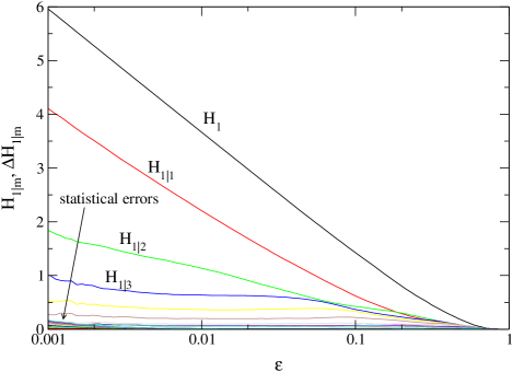
Figure 4: (Color online) Conditional entropies of the Mackey-Glass dynamics with effective delay $K=6$

Even though in Fig.4 for usual (nonperforated) conditional entropies the delay is invisible, the entropic-statistical criterion (29) selects it. This is seen in Fig.5, where a whole series of optimal perforated Markov models for different effective delays is shown.

Figure 5: Resolution-dependent optimal perforated Markov models for the Mackey-Glass dynamics with different effective delays $K$.

The right part of the panels is again subject to coarse graining effects. For higher resolution more structure is visible. The most important point to stress is that all panels have in common that there is an interval of resolutions, where the optimal perforated Markov model contains omissions behind the first step of conditioning and the first following time step taken into account is exactly the time step corresponding to the effective delay of the dynamics. The index 0 is always part of ${\bf{J}}^{*}(\epsilon)$, because of the $x_{n}$-term in Eq.(36).

Concluding, the very long range of the memory of the Mackey-Glass system requires strong downsampling, from which the complication arises that the resulting effective memory underlies some smearing effects. Nevertheless, since it was detected by the criterion, also this example has to be interpreted as a successful test of the criterion.

Without going into detail here it should be mentioned that in holstdiss07 various further variants for the selection of conditioning components as e.g. a restricted cardinality of conditioning components or a priori omissions of indices were suggested, in order to reach the further past for detection of potential memory.

VIII Consequences for prediction

VIII.1 Point prediction and prediction error

General point prediction one time step into the future reads

$$\hat{x}_{n+1}=F(\mathbf{x}_{n})$$ (39)

with a suitably chosen function $F$. The average quality of predictions can be evaluated by an accuracy measure. We choose the root mean squared (rms) prediction error given by

$$\hat{e}=\sqrt{\overline{(x_{n+1}-\hat{x}_{n+1})^{2}}}\;.$$ (40)

As a consequence the mean value of the estimated distribution of $X_{n+1}$, the random variable corresponding to the measured value $x_{n+1}$, is the optimal $F$. This distribution is estimated by a selected set of $x_{k+1}$, which are obtained from those $\mathbf{x}_{k}$, which are in some sense suitably related to $\mathbf{x}_{n}$. A decision, what a ’suitable relation’ should be, is not immediately given by Eq.(40) and has to be made additionally. Another possible accuracy measure could be the mean absolute error, which would lead to an optimal $F$ given by the median. In general the prediction error depends on the lead time (time into the future), the dataset length $N$, the noise in the dynamical modeling $F$ and possibly on the resolution $\epsilon$.

VIII.2 Locally constant prediction with generalized delay vectors

A special point prediction used in the following, which is locally constant (cmp. the zeroth order predictor in farmer87 ) and perforated, reads

$$\hat{x}_{n+1}(\epsilon) =\frac{\sum_{k\neq n}\Theta(\epsilon-\|P_{\bf{J}}\mathbf{x}_{n}-P_{\bf{J}}\mathbf{x}_{k}\|)\cdot x_{k+1}}{\sum_{k\neq n}\Theta(\epsilon-\|P_{\bf{J}}\mathbf{x}_{n}-P_{\bf{J}}\mathbf{x}_{k}\|)}$$

$$=\!\frac{1}{|\{P_{\bf{J}}\mathbf{x}_{k\neq n}\in{\mathcal{U}}(\epsilon,P_{\bf{J}}\mathbf{x}_{n})\}|}\!\!\sum_{P_{\bf{J}}\mathbf{x}_{k\neq n}\in{\mathcal{U}}(\epsilon,P_{\bf{J}}\mathbf{x}_{n})}\!\!\!\!\!\!\!\!x_{k+1}\;.$$ (41)

$P_{\bf{J}}$ is the projection operator onto the perforation structure given by the set ${\bf{J}}$ already encountered in Sec.V and ${\mathcal{U}}(\epsilon,P_{\bf{J}}\mathbf{x}_{n})$ is the $\epsilon$-neighborhood of the vector $P_{\bf{J}}\mathbf{x}_{n}$ introduced in Eq.(10). Apart from the perforatedness the method is also called the Lorenz method of analogues: The predicted future value is the mean of the known futures of similar states from the past. We will study explicitly the resolution dependence of the corresponding prediction error:

$$\hat{e}(\epsilon)=\sqrt{\overline{(x_{n+1}-\hat{x}_{n+1}(\epsilon))^{2}}}\;.$$ (42)

VIII.3 Example: Prediction from optimal perforated Markov model for generalized Henon dynamics

After having found the optimal resolution-dependent perforated Markov models from the criterion (29) with the suitable balance $b$, the corresponding component structures given by ${\bf{J}}^{*}(\epsilon)$ can be used for the calculation of point predictions according to Eq.(VIII.2) and rms prediction errors according to Eq.(42). In the following the prediction error corresponding to the optimal perforated Markov model, i.e., conditioning in the sense of the optimal generalized delay vector (GDV), is compared to the minimum of the prediction error of usual standard embeddings (1 - 5 delay vector (DV) components in presence and past; delay of 1 - 5 time steps). As an example we treat the generalized Hénon map

$$y_{n+1}=a-y_{n-K+2}^{2}-cy_{n-K+1}\;,$$ (43)

a simple chaotic system introduced by Baier&Klein in baier90 . In general it contains longer memory than the usual Hénon map

$$x_{n+1}=1-\alpha x_{n}^{2}+\beta x_{n-1}\;,$$ (44)

which is obtained from the generalized Hénon map in the case of $K=2$ from the transformation $y=ax$, $a=\alpha$ and $c=-\beta$. The nonlinearity still arises from one single quadratic term. The coefficients are chosen to be $a=1.76$ and $c=0.1$. From comparison of the coefficients $1$ vs. $c$ of the non-constant terms of Eq.(43) it is possible to see in this case that the linear term is suppressed in importance. From the choice of the delay $K=4$ the structure of dependence can be indicated by the set ${\bf{J}}_{0}=\{-3,-2\}$.

In Fig.6 results for prediction (lower panel) from optimal perforated Markov models (upper panel) are shown for the generalized Hénon map for a balance factor of $b=4$ in (29) which favors models with fewer components. It is seen that the prediction error from the optimal perforated Markov model is smaller than the minimum of prediction errors from standard embeddings. This serves as a justification for the introduction of perforatedness into the framework of Markov approximations and for practical applicability of the criterion (29) for prediction purposes.

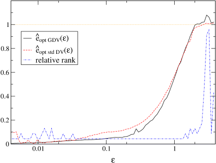
Figure 6: (Color online) Upper panel: Optimal resolution-dependent perforated Markov model (${\bf{J}}^{*}(\epsilon)$) for a dataset of $N=10000$ data points of the generalized Hénon with delay $K=4$. Lower panel: Resolution-dependent prediction error $\hat{e}_{\operatorname{opt\,GDV}}(\epsilon)$ from ${\bf{J}}^{*}(\epsilon)$, minimal prediction error $\hat{e}_{\operatorname{opt\,std\,DV}}(\epsilon)$ of standard delay vectors and relative rank of the prediction error from ${\bf{J}}^{*}(\epsilon)$ in the list of prediction errors from standard embeddings.

IX Conclusion

For dynamics with potentially infinite memory, e.g. from projection of stochastic dynamics into one measurement quantity, novel criteria for optimal Markov approximations were introduced. It was realized that essentially two types of errors are relevant: First, a modelling error, quantified by the ignored memory, and second, a statistical error of uncertainty reduction, quantified by the statistical error of the redundancy.

Usually Markov approximations are accompanied by losses of information, which become less the more memory is taken into account. Exactly the opposite holds for the statistical error of the uncertainty reduction, because a larger Markov order causes stronger restrictions in neighbor search algorithms responsible for larger statistical errors in the estimation of entropies and hence also of the redundancy. The rather simple idea behind the criterion for usual Markov approximations is that it makes no sense to further reduce ignored memory if the statistical error of the uncertainty reduction is already larger. Here the monotony properties of the involved quantities were used in the mathematical formulation of the criterion.

Even though this criterion was successfully applicable on simple dynamics, problems arise from the huge statistical errors for high cardinality of conditioning sets for dynamics with long range and inhomogeneously distributed memory. Hence, a generalization to a perforated case, where omissions of time steps in the past have to be allowed, was needed. A generalized notational framework of information theory in time series analysis was developed, which in principle allows for a unified description of variable future time steps ahead, jointly conditioned joint uncertainties, regular perforation (downsampling) and arbitrary irregular perforation with the tools of information theory. On this basis a novel criterion for optimal perforated Markov approximations was introduced, in which the selection algorithm for relevant conditioning components took into account the nonexistence of monotony properties of the modelling error in the cardinality of the conditioning set.

The perforated criterion was successfully tested for linear stochastic (AR) and nonlinear deterministic (Mackey-Glass) dynamics. It was found that the optimal perforated Markov model is resolution-dependent. For certain intervals of intermediate resolution the memory structure of the dynamical law was retrieved by the suggested criterion indicating the functional capability to yield suitable Markov approximations. For small resolutions coarse graining effects are clearly seen and for fine resolutions from statistical reasons fewer conditioning components are selected. The importance of the dependence on the length of the underlying dataset was pointed out.

Since the methods are based exclusively on quantities from information theory and statistical errors in their estimation, in particular the perforated variant is applicable to a broad class of dynamics. This is especially useful for an analysis of data sets, where it is not allowed to assume nice properties like, e.g., linearity. The explicit calculation of the statistical error of entropies made accessible those criteria based only on entropies and its derived quantities. In spite of the success of the criterion on the example dynamics, it has to be mentioned that nonstationarity and intermittency still remain as problems.

For locally constant and perforated point prediction an explicitly resolution-dependent root mean squared prediction error was introduced. For certain resolutions an improvement of the rms prediction error from the resolution-dependent optimal perforated Markov model in comparison with the rms prediction error from standard embeddings was seen in the example of the generalized Hénon map.

References

- (1) F. Takens, in Lecture Notes in Mathematics 898 (Springer, Berlin, 1981), 366.
- (2) F. Paparella, A. Provenzale, L. A. Smith, C. Taricco, and R. Vio, Phys. Lett. A 235, 233 (1997).
- (3) H. Kantz, D. Holstein, M. Ragwitz, and N. K. Vitanov, Physica A 342, 315 (2004).
- (4) B. W. Silverman, Density Estimation for Statistics and Data Analysis (Chapman & Hall, London, 1992).
- (5) T. Sauer, T. Yorke, and M. Casdagli, J. Stat. Phys. 65, 579 (1991).
- (6) P. Grassberger and I. Procaccia, Phys. Rev. A 28, 2591 (1983).
- (7) R. Friedrich and J. Peinke, Phys. Rev. Lett. 78, 863 (1997).
- (8) S. P. Garcia and J. S. Almeida, Phys. Rev. E 71, 037204 (2005).
- (9) L. M. Pecora, L. Moniz, J. Nichols, and T. L. Carroll, Chaos 17, 013110 (2007).
- (10) P. Grassberger, arXiv:physics/0307138 (2003).
- (11) D. Holstein, Ph.D. thesis, University of Wuppertal, 2007.
- (12) M. C. Mackey and L. Glass, Science 197, 287 (1977).
- (13) P. Grassberger and I. Procaccia, Physica D 9, 189 (1983).
- (14) J. D. Farmer, Physica D 4, 366 (1982).
- (15) J. D. Farmer and J. J. Sidorovich, Phys. Rev. Lett. 59, 845 (1987).
- (16) G. Baier and M. Klein, Phys. Lett. A 151, 281 (1990).