Heterogeneous expectations and long range correlation of the volatility of asset returns

Abstract

Inspired by the recent literature on aggregation theory, we aim at relating the long range correlation of the stocks return volatility to the heterogeneity of the investors’ expectations about the level of the future volatility. Based on a semi-parametric model of investors’ anticipations, we make the connection between the distributional properties of the heterogeneity parameters and the auto-covariance/auto-correlation functions of the realized volatility. We report different behaviors, or change of convention, whose observation depends on the market phase under consideration. In particular, we report and justify the fact that the volatility exhibits significantly longer memory during the phases of speculative bubble than during the phase of recovery following the collapse of a speculative bubble.

JEL classification: G10, G14, D84, C43, C53

Keywords: Realized volatility, aggregation model, long memory, bounded rationality

Introduction

The slow hyperbolic decay of the auto-correlation function characterizing the behavior of many economic and financial time series has been the topic of active debates for more than two decades. Several interpretations and models have been provided in an attempt to explain the origin of this phenomenon, also known as the long-memory phenomenon. Among the most relevant explanations that have been proposed up to now, one can focus on three major mechanisms acting separately or in conjunction: (i) the aggregation approach suggested by granger80 who have shown that the time series resulting from the aggregation of micro-variables exhibiting short-memory often yields long-memory, (ii) the presence of infrequent structural breaks, which allows mimicking long term non-stationarity of the economic and financial activity [diebold01, gourieroux01, granger04, gadea04, among others], and (iii) the presence of non-linearities in economic an financial systems (see davidson05 for a survey).

Our aim, in this article, is to provide a model that relates the long memory of the realized volatility of assets returns, which is a pervasive feature of financial time series [Taylor86, ding83, Dacorogna93, for the pioneering works], to the heterogeneous behavior of the economic agents. Based on the fact that the market participants perform heterogeneous anticipations about the future level of the realized volatility and that they act as bounded rationality agents, we propose an explanation of the long memory phenomenon that relies on the aggregation by the market of the heterogeneous beliefs of the investors, revealed through the market pricing process.

The heterogeneity of market investors is now an well-recognized fact – in particular amongst the supporters of behavioral finance (see BT2003 for a survey) – that can take several forms. Heterogeneity can first be considered as resulting from the diversity of the nature, the size and strategies of the economic agents: individual investors who invest their money to finance the education of their children, traders who manage money for their own account or for the account of their clients, institutional investors who manage pension funds, and so on… do not have the same financial resources (depending on their size), the same purposes (short term or long term profits and allocation frequency for example), or the same skills. All these differences make them focusing on different pieces of information and therefore anticipating differently the future value of the firms.

In this respect, Dacorogna05 have recently provided evidence for the existence of a relation between the degree of heterogeneity amongst the market participants and the stage of development of financial markets. Indeed, relating the stage of maturity of a financial market to the speed of the hyperbolic decay of the auto-correlation function of the volatility of the assets traded on the market under consideration, Di Matteo et al. suggest that the more mature and efficient the market is, the larger is the number of different classes of agents and strategies and the smaller is the effect of long-memory. In addition, other phenomena such as mass psychology and contagion must be taken into account. Indeed, clear evidence has shown that rumors [banerjee93], mimetism [orlean95], herding [banerjee92, froot92, kirman93, cont00], fashions [shiller89] and so on, affect the agents’ behavior.

In order to account for these various sources of heterogeneity but still keep a parsimonious representation, we provide a model that relates the investors’ behavior to few heterogeneity parameters that allow accounting for their individual tendency to perform optimal anticipations on the basis of the flow of incoming news they receive or, on the contrary, on the basis of a self-referential approach which leads them to mainly focus on their past anticipations and on their past observations of the market volatility. This approach permits us to focus on the fact that, in addition to the heterogeneity of sizes and strategies, another main source of heterogeneity comes from the way the agents actually anticipate the many factors which impact future earnings of the firm and their volatility. These factors are captured, in our model, by help of a flow of incoming public and private information which can be considered as embedding several macroeconomic variables affecting stocks volatility such as the business cycles (see schwert89 who has found a higher volatility of many key economic variables during the Great Recession), oil price whose volatility is important in explaining technology stock return volatility [sadorsky03], or inflation and interest rates which have large impacts on the stock market volatility [kearney98].

Then, we make the connection between the distributional properties of the heterogeneity parameters and the auto-covariance/auto-correlation functions of the realized-volatility. It allows us to discuss the kind of economic behaviors that yields the long memory of the realized-volatility time series. Finally, the calibration of our model over the last decade, on a database of 24 US stocks of large and middle capitalizations, allows us reconstructing the distribution of the heterogeneity parameters and then to have access to the overall behavior of the investors. Notably different behaviors are observed, depending on the market phase under consideration with (i) a strong tendency to self-referential anticipations before the crash of the Internet bubble, and (ii) a redistribution in favor of the investors performing their forecasts on the basis the incoming piece of information after the crash.

The paper is organized as follows. The next section briefly recalls some basic stylized facts about the so-called realized-volatility, a measure of the volatility introduced by andersen02 and barndorff01, among others. Then in section 2, we present our model of bounded rationality investors with heterogeneous beliefs in order to investigate the impact of both the agents’ bounded rationality and their heterogeneous beliefs in a market that is assumed to perform an aggregation of the individual anticipations. In section 3, we discuss the calibration issues of the model and derive the asymptotic law of the estimator of the parameters of the model. The fourth section present our empirical results while the fifth section concludes.

1 Stylized facts about the realized volatility of asset prices

Many stylized facts about the volatility of financial asset prices have been reported in several studies over the recent years [ding83, lo91, among many others]. In particular, people now agree on the fact that (i) returns display, at any time scale, a high degree of variability which is revealed by the presence of irregular bursts of volatility and (ii) the volatility displays a positive auto-correlation over large time lags, which quantifies the fact that high (resp. low) volatility events tends to cluster in time, as already reported by mandelbrot63 and fama65 who first mentioned evidence that large changes in the price of assets are often followed by other large changes, and small changes are often followed by small changes. This behavior has also been noticed by several other studies, such as baillie96, chou88 or schwert89 for instance.

In this section, after we have recalled the definition of the notion of realized volatility, we document some of the common features of the process of the asset price realized volatility and relate them to the relevant literature.

1.1 Definition of the realized volatility

Based upon the quadratic variation theory within a standard frictionless arbitrage-free pricing environment, andersen02 have suggested a general framework for the use of high frequency data in the measurement, the modeling and the prediction of the daily volatility of asset returns. In fact, as also recalled by barndorff01 barndorff01,barndorff02, when the underlying asset price process is a semi-martingale, the realized variance (the squared realized volatility) provides a consistent estimator of the quadratic variation, in the limit of large samples. Indeed, denoting by $P_{i,t}$ the $i^{th}$ observation of the asset price during the trading day $t$ and by $r_{i,t}=\ln(P_{i,t})-\ln(P_{i-1,t})$ the continuously compounded return on the asset under consideration over the period $i-1$ to $i$, the realized variance, at day $t$, defined by

$$\hat{\sigma}_{t}^{2}=\sum_{i=2}^{n_{t}}r_{i,t}^{2},$$ (1)

with $n_{t}$ the number of observations during this day, is a consistent estimator of the integrated variance of the price process. In addition, as shown by barndorff01, the asymptotic properties of this estimator are such that

$$\frac{\hat{\sigma}_{t}^{2}-\int_{t_{1}}^{t}\sigma^{2}(s)~{}ds}{\sqrt{\frac{2}{3}\displaystyle\sum_{i=1}^{n_{t}}r_{i,t}^{4}}}\stackrel{{\scriptstyle{\cal L}}}{{\longrightarrow}}{\cal N}(0,1),\qquad\text{and}\qquad\frac{\ln\hat{\sigma}_{t}^{2}-\ln\int_{t_{1}}^{t}\sigma^{2}(s)~{}ds}{\sqrt{\frac{2}{3}\displaystyle\frac{\sum_{i=1}^{n_{t}}r_{i,t}^{4}}{\left[\sum_{i=1}^{n_{t}}r_{i,t}^{2}\right]^{2}}}}\stackrel{{\scriptstyle{\cal L}}}{{\longrightarrow}}{\cal N}(0,1),$$ (2)

where $\sigma(t)$ is the instantaneous (or spot) volatility of the log price process.

If the estimator (1) does not require the time series of asset returns to be homoscedastic during day $t$, it is however assumed that the returns are uncorrelated. Therefore, in order to account for the market microstructure effects, which may produce spurious correlations [roll84, for instance], it is often necessary either to filter the raw series of intraday returns to remove these correlations or to focus on sufficiently large time scales – 5 minutes instead of 1 minute or tick by tick quotations, for instance – in order to smooth out the microstructure effects and correlations. The immediate drawback of this later approach is to decrease the number $n_{t}$ of available observations, which may bias the estimates.

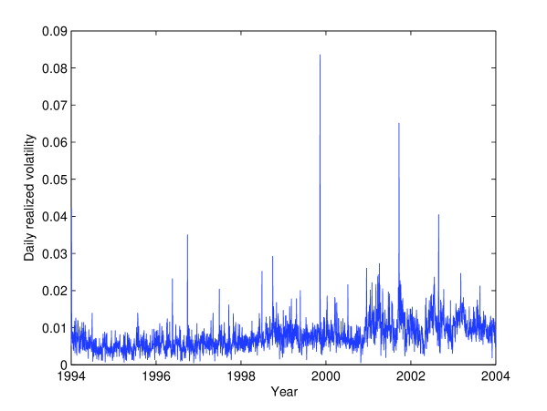
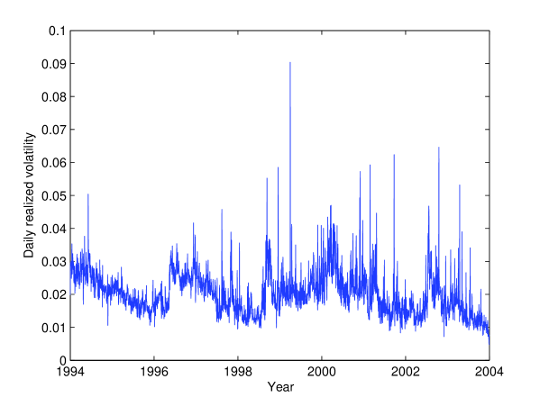
Figure 1: Daily realized volatility of two assets from 01/01/1994 to 12/31/2003. On the left a middle capitalization : The Washington Post, and on the right a large capitalization : Coca Cola.

[Insert figure 1 about here]

As an illustration, we present, on the figure 1, the realized volatility for two time series drawn from our intraday database of 24 US stocks prices (see section 4 for details on the database). On the left panel, we can observe the realized volatility of the daily returns of a middle capitalization stock (The Washington Post) during the time period from 01/01/1994 to 12/31/2003 while, on the right panel, is depicted the realized volatility of a large capitalization stock (Coca-Cola) over the same time period. Since our investigation of the time dependence between the intraday returns of these asset prices has not revealed the presence of a significant correlation beyond the one minute time scale, the market microstucture effect are negligible, which allows us to directly estimate the realized volatility from the one-minute raw returns.

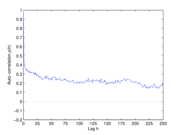
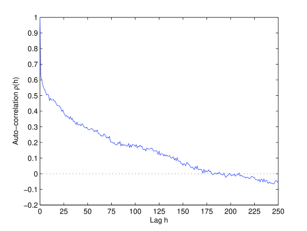
Figure 2: Auto-correlation function of the realized volatility of two assets from 01/01/1994 to 12/31/2003. On the left a middle capitalization : The Washington Post, and on the right a large capitalization : Coca Cola.

[Insert figure 2 about here]

On the figure 2, we have drawn the auto-correlation function of the previous realized volatility (still The Washington post on the left and Coca-Cola on the right) from lag 0 to lag 250 days, which corresponds to a one year period or so. The slow decay is characteristic of the long memory. However, the two graphs seem different. For The Washington Post the auto-correlation falls down to 0.4 quickly and then decreases very slowly, whereas for Coca-Cola, it decreases more regularly and the auto-correlation becomes not significantly different from zero beyond lag 180, or so. This general feature could mean that the correlation function of the volatility of large capitalization stocks would exhibit shorter memory than middle capitalization stocks. This remark, that will be confirmed later, is in line with the observation reported by Dacorogna05 and according to which the more efficient a stock (or a market), the faster the decay of the correlation function of its volatility.

1.2 Normality of the log-volatility

We now turn to the distributional properties of the realized volatility. As suggested by many previous studies [andersen01, andersen01b, barndorff02, among others], the log-normal distribution provides an adequate description of the distribution of the volatility, at least in the bulk of the distribution. These observations clearly support the modeling of the realized volatility in terms of log-normal models, which goes back to clark73 (see also Taylor86).

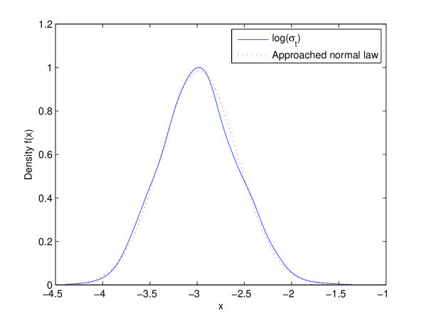
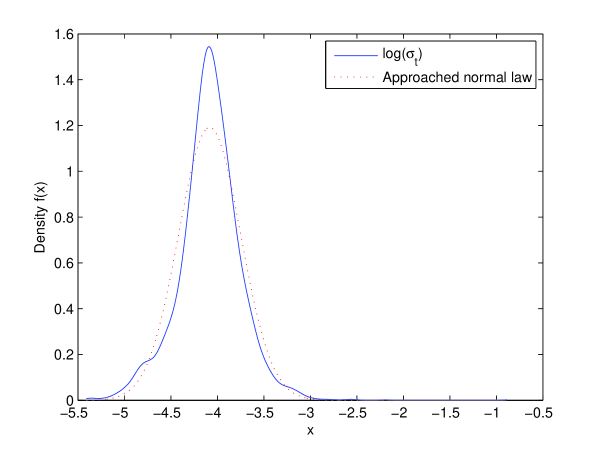
Figure 3: Density of $\log(\hat{\sigma}_{t})$ and their approached normal law for different assets. On the left a middle capitalization : Microchip Technology inc., and on the right a large capitalization : Procter & Gamble co.

Starting from these observations, let us illustrate the relevance of the log-normal model for the realized volatility of the returns on the prices of the assets in our database. To this aim, let us denote by $\{\omega_{t}\}_{t\geq 1}$ the logarithm of the series of the realized volatility. Figure 3 shows the kernel estimate [pagan99] of the density of the log-volatility of a mid-cap (Microchip Technology) on the left panel and of a large cap (Coca Cola) on the right one, over the whole time period. The density of log-volatility of the price returns of Microchip Technology seems very close to a normal density at the naked eye. On the overall, it is the case for all the mid-caps. On the contrary, the densities of the large caps present sharp peaks and fat tails so that they significantly depart from the normal density. These visual impressions will be formalized later on, in section 4.

[Insert figure 3 about here]

2 Heterogeneity model

As recalled in introduction, several explanations have been proposed, in the now large body of literature about the long memory of financial time series, to point out the various origins of this phenomenon. The first one, addressed by granger80, concerns the nature of financial time series. Indeed, they consider that financial series results from the aggregation of micro-variables and that this aggregation is responsible for the long memory. The second one is the presence of infrequent structural breaks (also called structural changes) in financial time series [diebold01, gourieroux01, granger04, gadea04, davidson05, among others].

Our model is based upon granger80’s proposition; it explains the long memory of the log-volatility of asset prices by the aggregation of micro-variables intended to represent the heterogeneous expectations of each market participant. For, we suppose that the market aggregates the agents’ anticipations of the log-volatility and that this aggregation drives the realized log-volatility. We will formalize this assumption later on.

2.1 General framework

The role of the log-volatility as the central object underpinning our model comes from the remark that, as recalled in the previous section, it is reasonable, in a first approximation, to consider that the realized volatility follows a log-normal distribution. As an additional hypothesis, we will assume that

(H1)          the log-volatility process $\{\omega_{t}\}_{t\in{\mathbb{Z}}}$ follows a Gaussian stochastic process,

which obviously ensures that the volatility itself has a log-normal stationary distribution.

Now, the standard economic theory tells us that any rational agent facing a decision problem aims at optimizing the output of her actions, based upon the entire set of information she has at her disposal. In the present context, it means that any rational investor strives for the best prediction of the future realized volatility $\hat{\sigma}_{t+\tau}$, $\tau\geq 1$, based on the set $\{\sigma_{1},\dots,\sigma_{t}\}$ of her past observations. In the sense of the minimum mean squared error, the best predictor is given by

$$\hat{\sigma}_{t+\tau} = \textrm{E}\left[\sigma_{t+\tau}|\sigma_{1},\dots,\sigma_{t}\right],$$ (3)

$$= \textrm{E}\left[\left.{\rm e}^{\omega_{t+\tau}}\right|\omega_{1},\dots,\omega_{t}\right],$$ (4)

$$= {\rm e}^{2\sigma_{\omega}(\tau)^{2}}\cdot{\rm e}^{\hat{\omega}_{t+\tau}},$$ (5)

where $\hat{\omega}_{t+\tau}$ denotes the best predictor of the log-volatility, based on the same set of observations and $\sigma_{\omega}(\tau)^{2}$ is the ($\tau$-step ahead) prediction error, i.e. the mean squared error $\textrm{E}\left[\left(\hat{\omega}_{t+\tau}-\omega_{t+\tau}\right)^{2}\right]$. Since the log-volatility is assumed to follow a Gaussian process, the best predictor $\hat{\omega}_{t+\tau}$ is given by a linear combination of the past observations and the past anticipations. In particular (see [pp. 162-168]brockwell90)

$$\hat{\omega}_{t+1}=\bar{\omega}+\sum_{i=0}^{t-1}\varphi_{t,i}\cdot\left(\hat{\omega}_{t-i}-\omega_{t-i}\right),$$ (6)

where the sequence of coefficients $\{\varphi_{t,i}\}_{i\geq 0}$ and the long term mean $\bar{\omega}$ depend on the specific model each investor relies on and on the particular calibration method she uses to estimate the structural parameters of her model. Thus, one expects that the $\varphi_{i}$’s are specific to each market actor so that each investor performs different expectations about the level of the future realized volatility. In addition, each agent can incorporate some exogenous economic variables or some piece of (private) information she thinks to improve her prediction.

Besides, considering that the market carries out an aggregation of the agents’ anticipations, we postulate that

(H2)          the realized log-volatility is the average of all the individual anticipations.

Thus, denoting by $\hat{\omega}_{i,t}$ the agent $i$’s forecast, the realized log-volatility is given by

$$\omega_{t}(n)=\frac{1}{n}\sum_{i=1}^{n}\hat{\omega}_{i,t},$$ (7)

if the market in made of $n$ participants. Under the assumption of an infinitely large number of investors, the realized log-volatility writes

$$\omega_{t}=\lim_{n\rightarrow\infty}\omega_{t}(n).$$ (8)

Our approach can appear utterly simplistic insofar as the real process yielding the realized volatility certainly involves non-linear transforms of the individual anticipations before they are actually aggregated through the price formation process, which is well-known to rely on various positive or negative feedback mechanisms [shiller00, sornette03]. However, in this first attempt to capture the impact of the heterogeneity of the investors’ anticipations on the dynamics of the realized volatility, and in the absence of arguments allowing us to model these non-linear interactions, it is necessary to restrict ourselves to this assumption of linearity.

Moreover, in order to be able to make tractable calculations, we need some other simplifying assumptions. Focusing on agent $i$, we denote by $\hat{X}_{i,t}$ its expectation about the future level of the excess log-volatility over its long term mean

$$\hat{X}_{i,t}=\hat{\omega}_{i,t}-\bar{\omega}$$ (9)

on day $t$, and by

$$\bar{X}_{n,t}=\omega_{t}(n)-\bar{\omega}=\frac{1}{n}\sum_{i=1}^{n}\hat{X}_{i,t}$$ (10)

the excess of the realized log-volatility over its long term mean. We assume that the anticipation $\hat{X}_{i,t}$ depends on the anticipation, $\hat{X}_{i,t-1}$, the agent made the day before and on the excess realized log-volatility $\bar{X}_{n,t-1}$, but also on a public piece of information $\varepsilon_{t}$ as well as on a private piece of information $\eta_{i,t}$ according to the recursion equation

$$\hat{X}_{i,t}=\varphi_{i}\cdot\hat{X}_{i,t-1}+\psi_{i}\cdot\bar{X}_{n,t-1}+c_{i}\varepsilon_{t}+\eta_{i,t}\qquad t\geq 0,\qquad i=1,2,\dots,n.$$ (11)

From equation (6), one should expect that $\psi_{i}=-\varphi_{i}$ if we consider rational agents who strive for the best prediction (in the minimum mean-squared sense) of the volatility. However, in order to generalize our model to the case where the market participants can be bounded rationality agents, we allows for $\psi_{i}\neq-\varphi_{i}$. Nonetheless, we will assume that these coefficients remains constant from time to time.

Let us stress that the first order dynamics (11) can seem too simple, and it probably is. However, our approach amounts to postulate that the agents assume that the (log)-volatility follows some kind of ARCH process, which is quite reasonable. In addition, even if real agents use more sophisticated prediction schemes to perform their expectations about the future level of the realized (log)-volatility, and thus use higher order dynamics, we can still make the assumption that these higher order dynamics can be reduced to an aggregation of first order dynamics. Therefore, $\hat{X}_{i,t}$ does not exactly characterize the expectation of individual agent but more precisely of a class of agents.

In this basic setting, the $n$-dimensional vector $\hat{X}_{t}=\left(\hat{X}_{1,t},\dots,\hat{X}_{n,t}\right)^{\prime}$ follows a first order (vectorial) auto-regressive process. The Gaussian noises $\{\varepsilon_{t}\}$, $\{\eta_{1,t}\}$, $\{\eta_{2,t}\}$, …, are independent, centered, and of variance $\textrm{Var}(\varepsilon_{t})=\sigma_{\varepsilon}^{2}$ and $\textrm{Var}(\eta_{i,t})=\sigma_{\eta_{i}}^{2}$, $\forall i$, respectively. Moreover the structural coefficients $\left(\varphi_{i},\psi_{i}\right)$ and $c_{i}$, which characterize the investors’ behavior, can be considered as the result of independent draws from the same law (called the heterogeneity distribution). These draws are independent of the values of the noises and the variables $\left(\varphi,\psi\right)$ and $c$ are independent of each other. The parameter $c$ that allows introducing heteroscedasticity must be strictly positive, while the distribution of $(\varphi,\psi)$ has to fulfill some hypotheses, which will be made explicit hereafter, in order to ensure the stationarity of the stochastic process $\{\hat{X}_{t}\}_{t\in{\mathbb{Z}}}$ and of the aggregated excess realized volatility $\{\bar{X}_{n,t}\}_{t\in{\mathbb{Z}}}$.

The appeal of the dynamic (11) rests on the simple interpretation that can be made of the structural coefficient $(\varphi,\psi)$ and of its distributional properties. It is obvious that the impact of the previous anticipation $\hat{X}_{i,t-1}$ on the current anticipation $\hat{X}_{i,t}$ depends on the value of the heterogeneity coefficient $\varphi_{i}$:

1. when $\varphi_{i}$ is close to (but less than) one, the impact of the previous anticipation on the current anticipation is very important and, unless a very large piece a information arrives – i.e. unless one observes a large $\varepsilon_{t}$ and/or a large $\eta_{i,t}$ – the current value of the expected excess log-volatility $\hat{X}_{i,t}$ will be very close to the previous one. On the overall, the agent believes in the continuity of the previous market conditions;

2. when $\varphi_{i}$ is close to (but larger than) minus one, the impact of the previous anticipation still remains more important than the arrival of a new piece of information, but the agent exhibits a systematic tendency to believe in the reversal of the volatility since her anticipation appears to be the opposite of the one she made the day before;

3. eventually, when $|\varphi_{i}|$ is close to 0, the anticipations are only scarcely related to those made the day before and mainly rely on the flow of incoming news.

To sum up, in the two first situations, we can notice that the market is highly self-referential: the impact of a new incoming piece of information remains weak, all the more so the closer to one the magnitude of $\varphi_{i}$. On the contrary, when $|\varphi|$ is close to zero, the degree of reactivity of the market participants to a new incoming piece of information is high. Thus, the magnitude of $\varphi$ can be seen as a way to quantify the degree of efficiency of the market. The same considerations obviously holds for $\psi_{i}$, but instead of referring to the past anticipation it refers to the publicly observed past realized volatility.

2.2 Properties of the (log-) volatility process

Equation (11) can be written in a more compact form as follows

$$\hat{X}_{t}=A\hat{X}_{t-1}+\varepsilon_{t}\cdot C+\eta_{t},$$ (12)

where $A=D+\frac{1}{n}\Psi\cdot 1_{n}^{\prime}~{}$ is an $n\times n$ matrix with $D={\rm diag}(\varphi_{1},\dots,\varphi_{n})$, $\Psi=\left(\psi_{1},\cdots,\psi_{n}\right)^{\prime}$ and $1_{n}=\underbrace{\left(1,\dots,1\right)^{\prime}}_{n~{}times}$, while $C=\left(c_{1},\dots,c_{n}\right)^{\prime}$ and $\eta_{t}=\left(\eta_{1,t},\dots,\eta_{n,t}\right)$. Besides, the range of the distribution of $(\varphi,\psi)$ is assumed to be such that the spectral radius of $A$ is less the one. This condition is necessary and sufficient to ensure the stationarity of the vectorial process $\{\hat{X}_{t}\}_{t\geq 0}$.

Under the assumption $||A||<1$, that will be assumed in all the sequel of this article, the stationary and causal solution of equation (12) is given by

$$\hat{X}_{t}=\sum_{k=0}^{\infty}A^{k}C\varepsilon_{t-k}+\sum_{k=0}^{\infty}A^{k}\eta_{t-k},$$ (13)

so that, as proved in appendix A:

Proposition 1.

In the limit of a large number of economic agents, $n\rightarrow\infty$, the excess realized log-volatility $\{\bar{X}_{t}\}_{t\in\mathbb{Z}}$ follows an infinite order auto-regressive moving average process

$$\left(1-\sum_{k=0}^{\infty}{\rm E}\left[\psi\varphi^{k}\right]L^{k+1}\right)\bar{X}_{t}={\rm E}\left[c\right]\cdot\left(\sum_{k=0}^{\infty}{\rm E}\left[\varphi^{k}\right]L^{k}\right)\varepsilon_{t},$$ (14)

where $L$ denotes the lag operator.

Not surprisingly, the flows of private information $\{\eta_{i,t}\}$ does not come into play since, under our assumptions, it does not convey any piece of information, on average across agents.

As a byproduct of the proposition above, we see that the solution to equation (14) can conveniently be expressed in terms of an infinite order moving-average provided that $\sum_{k=0}^{\infty}\textrm{E}\left[\psi\varphi^{k}\right]z^{k+1}\neq 1$ for all $z$ inside the unit circle:

$$\bar{X}_{t}=\textrm{E}\left[c\right]\cdot\sum_{k=0}^{\infty}\tilde{\beta}_{k}\varepsilon_{t-k},$$ (15)

where the $\tilde{\beta}_{k}$’s are formally given by the coefficients of the power series

$$\sum_{k=0}^{\infty}\tilde{\beta}_{k}x^{k} := \displaystyle\textrm{E}\left[\displaystyle\frac{1}{1-x\cdot\varphi}\right]\left(\displaystyle 1-x\textrm{E}\left[\frac{\psi}{1-x\cdot\varphi}\right]\right)^{-1}~{},$$ (16)

$$= \displaystyle\textrm{E}\left[\displaystyle\frac{1}{1-x\varphi}\right]\left(\displaystyle 1-\textrm{E}\left[\frac{xg(\varphi)}{1-x\varphi}\right]\right)^{-1}~{},$$ (17)

where $g(\varphi)=\textrm{E}[\psi|\varphi]$.

The process $Y_{t}:=\left(\sum_{k=0}^{\infty}\textrm{E}\left[\varphi^{k}\right]L^{k}\right)\varepsilon_{t}$, is stationary if and only if $\sum_{k=0}^{\infty}\textrm{E}\left[\varphi^{k}\right]^{2}<\infty$, which requires that the law of $\varphi$ be concentrated on $(-1,1)$. It is however not sufficient, as shown by goncalves88. Furthermore, $Y_{t}$ exhibits long memory provided that $\sum_{k=0}^{\infty}|\textrm{E}\left[\varphi^{k}\right]|=\infty$. Restricting our attention to the case where $Y_{t}$ is said to exhibit long memory if its spectral density

$$f_{Y}(\lambda)=\frac{\sigma_{\varepsilon}^{2}}{2\pi}\left|\sum_{k=0}^{\infty}\textrm{E}\left[\varphi^{k}\right]e^{-ik\lambda}\right|^{2}\sim\lambda^{-2d_{Y}},\quad d_{Y}\in\left(-\frac{1}{2},\frac{1}{2}\right),$$ (18)

we conclude that the density of $\varphi$ – if it exists – should behave as $(1-\varphi)^{-d_{Y}}$ as $\varphi$ goes to one. Actually, $Y_{t}$ exhibits long-memory if $d_{Y}\in(0,1/2)$ and anti-persistence if $d_{Y}\in(-1/2,0)$. The upper bound on $d_{Y}$ is necessary in order for the process to be second order stationary.

As for the filter $A(L):=1-\sum_{k=0}^{\infty}\textrm{E}\left[\psi\varphi^{k}\right]L^{k+1}$ in the left-hand side of (14), it is well defined if $\sum_{k=0}^{\infty}\textrm{E}\left[\psi\varphi^{k}\right]^{2}<\infty$ which, by Cauchy-Schwartz inequality, is satisfied if $\textrm{E}\left[\psi^{2}\right]<\infty$ and $\sum_{k=0}^{\infty}\textrm{E}\left[\varphi^{2k}\right]<\infty$. This requirement is, however, not necessary. As a further hypothesis, we will assume that $\sum_{k=0}^{\infty}\textrm{E}\left[\psi\varphi^{k}\right]^{2}x^{k+1}\neq 1$ for all $x\in[-1,1]$ which ensures that $A(z)$ does not vanish for any $z$ inside the unit circle. The behavior of $A(z)$, as $z$ goes to one, depends on the conditional expectation of $\psi$ given $\varphi$, namely $g(\varphi):=\textrm{E}\left[\psi|\varphi\right]$. Either $A(z)$ remains finite as $z\to 1$, and $X_{t}$ exhibits long memory if and only if $Y_{t}$ itself exhibits long memory or $A(z)$ diverges hyperbolically, as $z\to 1$, and the memory (short or long) of the log-volatility process results from a mix between the properties of the distribution of $\varphi$ and of the conditional expectation $g(\varphi)$. More precisely, we can state that (see the proof in Appendix B)

Proposition 2.

Under the assumptions above, if the density of $\varphi$ is $f(\varphi)\sim(1-\varphi)^{-\alpha}$, $\alpha\in(0,1/2)$, and if the conditional expectation of $\psi$ given $\varphi$ is $g(\varphi)\sim(1-\varphi)^{\beta}$, $\beta>\alpha-1/2$, as $\varphi\to 1^{-}$, the spectral density of the log-volatility process behaves as $f_{X}(\lambda)\sim\lambda^{-2\min\{\alpha,\beta\}}$, as $\lambda\to 0$.

As an illustration of this result, let us assume that $\varphi\stackrel{{\scriptstyle law}}{{=}}$ Beta$(-\alpha,1+\alpha)$. We deduce that $\textrm{E}\left[\frac{1}{1-x\varphi}\right]=(1-x)^{\alpha}.$ If, in addition, we assume that $\textrm{E}[\psi|\varphi]=(1-\varphi)^{\beta}$, we get $\textrm{E}\left[\frac{g(\varphi)}{1-x\varphi}\right]=\frac{\Gamma(1+\alpha+\beta)}{\Gamma(1+\alpha)\Gamma(1+\beta)}F(1,-\alpha;1+\beta;x),$ where $F$ is the hypergeometric function (see abramowitz65 for the definition). Thus, equation (16) writes

$$\sum_{k=0}^{\infty}\tilde{\beta}_{k}x^{k}=\frac{(1-x)^{\alpha}}{\displaystyle 1-\frac{\Gamma(1+\alpha+\beta)}{\Gamma(1+\alpha)\Gamma(1+\beta)}xF(1,-\alpha;1+\beta;x)}.$$ (19)

Under the assumption that $\beta>1$, which assures that the denominator in equation (19) remains bounded for all $|x|\leq 1$, the series $\sum_{k=0}^{\infty}\tilde{\beta}_{k}x^{k}$ behaves like $C(1-x)^{\alpha}$ in the neighborhood of 1 and thus diverges hyperbolically if $\alpha<0$. The expression of the spectral density is then deduced from equations (15) and (19):

$$f_{X}(\lambda)=\frac{\textrm{E}\left[c\right]^{2}\sigma_{\varepsilon}^{2}}{2\pi}\frac{|1-e^{-i\lambda}|^{2\alpha}}{\left|1-\frac{\Gamma(1+\alpha+\beta)}{\Gamma(1+\alpha)\Gamma(1+\beta)}e^{-i\lambda}F(1,-\alpha;1+\beta,e^{-i\lambda})\right|^{2}}$$ (20)

and, since $f_{X}(\lambda)\underset{\lambda\rightarrow 0}{\sim}C^{\prime}|\lambda|^{2\alpha}$, the auto-correlation function reads $\rho(h)\sim K|h|^{-2\alpha-1}$ as $|h|\rightarrow\infty$, provided that the second order stationarity condition $\alpha>-1/2$ holds.

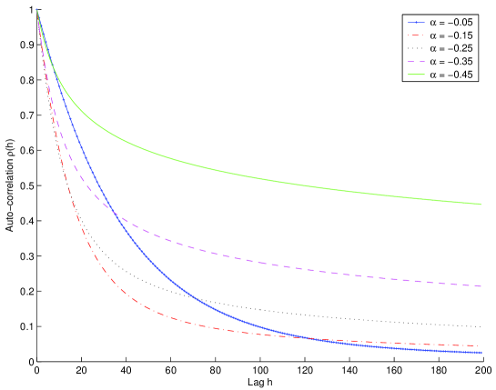
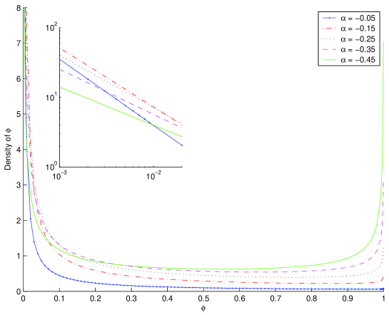
Figure 4: The left panel and the right panel represent respectively the auto-correlation function over 200 days and the density of the heterogeneity coefficient $\alpha$ for different values of $\alpha$ ranging in $[-0.45,-0.05]$ and $\beta=1.5$. The law of $\varphi$ is a Beta($-\alpha$,$1+\alpha$) and its density equal to $f(\varphi)=\frac{1}{B(-\alpha,1+\alpha)}\varphi^{-\alpha-1}(1-\varphi)^{\alpha}$ explains the divergence near 0 and 1.

For the sake of completeness, let us discuss the role played by the two parameters $\alpha$ and $\beta$ in the model. As $\varphi$ is assumed to follow a Beta($-\alpha,1+\alpha$) law, then $\textrm{E}[\varphi]=-\alpha\in[-0.5,0]$. It implies that the anticipation of an agent is not mainly based on her past anticipation. Recall that $|\varphi|$ should be close to one in order to observe a strongly self-referential behavior. In other words, the agents attach more importance to the realization of the past volatility and to the information flows, on average. The closer $\alpha$ to 0, the less importance is given to the past anticipation. Consequently, as the anticipations of the agents are more based on common facts (past realized volatility and informations), then the heterogeneity of the agents’ beliefs decreases. As a conclusion the long memory should decrease. This phenomenon is shown on the left panel of figure 4, where auto-correlation functions for a fixed $\beta=1.5$ and different values of $\alpha$ ranging in $[-0.45,-0.05]$ are drawn.

[Insert figure 4 about here]

The right panel of figure 4 shows the densities of $\varphi$ for the same set of values of $\alpha$. This figure confirms that the closer $\alpha$ to -0.5, the stronger is the divergence near 1. It means that the relative proportion of agents attaching importance to their past anticipation increases and thus the long memory increases. Furthermore, we notice that the speed of the decrease of the auto-correlation function and the divergence of the density function are strongly related. It means that $\alpha$ impacts both on short and long memory, which is not a surprise since – with our simple parameterization – $\alpha$ controls both the behavior of the density of $\varphi$ close the one and in the neighborhood of zero.

As for $\beta$, in order to illustrate its role, we focus on the other heterogeneity parameter $\psi$ whose mean is $\textrm{E}[\psi]=\frac{\Gamma(1+\alpha+\beta)}{\Gamma(1+\alpha)\Gamma(1+\beta)}$. The limits of $\textrm{E}[\psi]$ when $\beta$ tends to 1 and to infinity are respectively $\textrm{E}[\psi]\underset{\beta\rightarrow 1}{\longrightarrow}1+\alpha$ and $\textrm{E}[\psi]\underset{\beta\rightarrow+\infty}{\longrightarrow}0$. So, the larger $\beta$, the closer $\psi$ to 0 on average.

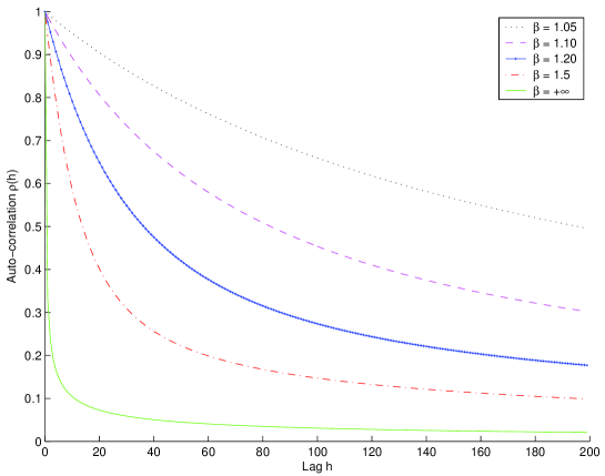
Figure 5: Auto-correlation function over 200 days for $\beta=1.5$ and different values of $\alpha$.

Now, by aggregation of the system (11), we obtain that the realization of the volatility on day $t$ is equal to a quantity depending on the past anticipations plus the past realization of the volatility times the mean of $\psi_{i}$ plus the information flows. Thus the aggregation of equation (11) could be interpreted as an an AR(1) process where $\textrm{E}[\psi]$ would be the auto-regressive coefficient. Even if the quantity depending on the past anticipations impacts on the short memory as we previously pointed out, all things being equal furthermore, when $\textrm{E}[\psi]$ decreases there are less short-term correlations and then the short memory falls. It is the reason why when $\textrm{E}[\psi]$ gets close to 0 (that is equivalent to $\beta$ tends to infinity), the short memory drops (see figure 5).

[Insert figure 5 about here]

2.3 Examples

Let us now discuss in details several typical examples of dynamics encompassed by our model and relate them with the agents’ behaviors.

2.3.1 Case 1: Rational agents

As recalled in the previous section, rational agents base their anticipations at time $t$ on the innovations $\hat{X}_{i,s}-\bar{X}_{n,s}$, $s\leq t-1$. Thus, setting $\psi_{i}=-\varphi_{i}$, for all $i=1,\ldots,n$ allows us to model the behavior of the realized volatility when the investors are fully rational agents since it allows us to retrieve the expression of the optimal predictor (6), in the particular case where the agents focus on the last innovation $\hat{X}_{i,t-1}-\bar{X}_{n,t-1}$ only. In this case, the dynamics on the individual anticipation writes

$$\hat{X}_{i,t}=\varphi_{i}\cdot\left(\hat{X}_{i,t-1}-\bar{X}_{n,t-1}\right)+c_{i}\cdot\varepsilon_{t}+\eta_{i,t}\qquad t\geq 0,\qquad i=1,2,\dots,n,$$ (21)

and by equation (16), we immediately obtain $\displaystyle\sum_{k=0}^{\infty}\tilde{\beta}_{k}x^{k}=1$, so that

$$\bar{X}_{t}=\textrm{E}\left[c\right]\varepsilon_{t}.$$ (22)

Notice, in passing, that we do not need each agent to be rational by setting $\psi_{i}=-\varphi_{i}$, but only that $\textrm{E}[\psi|\varphi]=-\varphi$ which means that the agents are not necessarily individually rational but only on average. Thus, if the agents are rational (individually or in average), the excess of the realized log-volatility only reflects the aggregated information, publicly available at time $t$, namely $\textrm{E}\left[c\right]\varepsilon_{t}$. This result is not surprising insofar as rational investors perform optimal anticipations and, therefore, the realized volatility can only convey the piece of information not present in the past innovation $\hat{X}_{i,t-1}-\bar{X}_{n,t-1}$. Then, since the information flow is assumed to be a white noise, the realized volatility should also be a white noise in the case where all the investors were rational.

2.3.2 Case 2 : Absence of heterogeneity

As a second basic example, let us assume that the investors only focus on the past realized volatility and completely neglect their past anticipations, i.e., $\varphi=0$. Consequently, the dynamics of the individual anticipations writes

$$\hat{X}_{i,t}=\psi_{i}\cdot\bar{X}_{n,t-1}+c_{i}\varepsilon_{t}+\eta_{i,t}\qquad t\geq 0,\qquad i=1,2,\dots,n.$$ (23)

By summation over all the agents $i$, and in the limit $n\rightarrow\infty$, one gets

$$\bar{X}_{t}=\textrm{E}\left[\psi\right]\cdot\bar{X}_{n,t-1}+\textrm{E}\left[c\right]\varepsilon_{t}\qquad t\geq 0,$$ (24)

which is a simple AR(1) process exhibiting only short memory since

$$\rho(h)=\textrm{E}\left[\psi\right]^{|h|}.$$ (25)

Thus, as noticed in the previous section, we remark again that the heterogeneity coefficient $\varphi$ is responsible for the long memory while $\psi$ mainly impacts the short memory. It clearly shows that the long memory phenomenon is rooted in the self-referential behavior of the investors, and more precisely in the self-reference to theirs own past anticipations and not to the past realized volatility.

2.3.3 Case 3: Absence of reference to the past realized volatility

At the opposite of the previous case, let us consider that each agent only bases her present anticipation on her past anticipation and on the flow of incoming news, but that she neglects the past realized volatility so that the dynamics of the individual anticipations reads

$$\hat{X}_{i,t}=\varphi_{i}\cdot\hat{X}_{i,t-1}+c_{i}\varepsilon_{t}+\eta_{i,t}\qquad t\geq 0,\qquad i=1,2,\dots,n,$$ (26)

and the expression of the $\tilde{\beta}_{k}$’s then simplifies to

$$\tilde{\beta}_{k}=\textrm{E}\left[\varphi^{k}\right],$$ (27)

which allows us to write the excess realized log-volatility and its auto-correlation function as

$$\bar{X}_{t}=\textrm{E}\left[c\right]\sum_{k=0}^{\infty}\textrm{E}\left[\varphi^{k}\right]\varepsilon_{t-k},\qquad\text{and}\qquad\rho(h)=\frac{\displaystyle\sum_{k=0}^{\infty}\textrm{E}[\varphi^{k}]\textrm{E}[\varphi^{k+h}]}{\displaystyle\sum_{k=0}^{\infty}(\textrm{E}[\varphi^{k}])^{2}},$$ (28)

provided that the stationarity condition $\displaystyle\sum_{k=0}^{\infty}(\textrm{E}[\varphi^{k}])^{2}<\infty$ holds.

It turns out that the properties of this dynamic has been investigated by goncalves88. Based on their result, one can remark, in passing, that this the correlation function, namely the auto-correlation function of the aggregated time series, is very different from the average correlation function $\bar{\rho}$. Indeed, before the aggregation, the auto-correlation function is of each individual agent’s expectation is

$$\rho_{i}(h)=\varphi_{i}^{|h|},\qquad i=1,2,\dots,\qquad h=0,1,\dots$$ (29)

so that

$$\bar{\rho}(h)=\textrm{E}[\varphi^{|h|}]\qquad h=0,1,\dots$$ (30)

Besides, the dynamics exhibits long memory if (and only if) the density of $\varphi$ diverges at one in order to get a hyperbolic decay of the correlation function (28). In other words, the density should behave like $(1-x)^{-d}$, $d<1/2$, in the neighborhood of one, that is to say like the density of the Beta law for instance, in order to obtain $\rho(h)\sim\lambda\cdot|h|^{2d-1}$, as $|h|$ goes to infinity. In such a situation, one can conclude that a significant part of the agents base their anticipations on the one they have made the day before.

2.3.4 Case 4: Deviation from rationality

Let us now focus on a particular case of bounded rationality agents. For, we assume $\psi=-\alpha\cdot\varphi+\bar{\varphi}^{\prime}$, where $\alpha$ and $\bar{\varphi}^{\prime}$ are two constants while $\varphi$ follows a “stretched” Beta$(p,q)$ law, namely a Beta$(p,q)$ law extended over the entire range $[-1,1]$. As we expect that the fraction of investors characterized by a heterogeneity parameter $\varphi_{i}$ close to one be larger and, in fact, diverges at 1, the parameter $p$ must be larger than one: $p>1$. On the contrary, we expect that the fraction of agents characterized by a heterogeneity parameter $\varphi_{i}$ close to minus one remains finite, so that $q$ must be smaller than one: $0<q<1$. The case of rational agents is obviously encompassed by this representation, since it corresponds to the situation where $\alpha=-1$ and $\bar{\varphi}^{\prime}=0$.

In this setting, the dynamics of the anticipation of the agent $i$ becomes

$$\hat{X}_{i,t}=\varphi_{i}\cdot\hat{X}_{i,t-1}+(\bar{\varphi}^{\prime}-\alpha\varphi_{i})\cdot\bar{X}_{n,t-1}+c_{i}\cdot\varepsilon_{t}+\eta_{i,t}\qquad t\geq 0,\qquad i=1,2,\dots,n.$$ (31)

and, from equation (16), the excess log-volatility $\bar{X}_{t}$ follows the infinite order moving-average (15) with coefficients $\tilde{\beta}_{k}$’s given by the relation

$$\sum_{k=0}^{\infty}\tilde{\beta}_{k}x^{k}=\frac{(1-x)^{q-1}G(p,q,x)}{1-\alpha+(\alpha-x\bar{\varphi}^{\prime})(1-x)^{q-1}G(p,q,x)},$$ (32)

where

$$G(p,q,x)=\begin{cases}(1+x)^{-q}\cdot F(p+q-1,q;p+q,\frac{2}{1+x^{-1}})&\text{if}~{}x\geq 0,\\ (1-x)^{-q}\cdot F(1,q;p+q,\frac{2}{1-x^{-1}})&\text{if}~{}x<0,\end{cases}$$ (33)

with $F(.,.;.,.)$ is the hypergeometric function. Two conditions are required in order for $G(p,q,x)$ to remain finite for all $|x|\leq 1$: $p>1$ and $0<q<1$. Since $0<q<1$, the numerator diverges. Let us study the behavior of the denominator, and figure out the conditions for its convergence.

$$\sum_{k=0}^{\infty}\tilde{\beta}_{k}x^{k}=\frac{G(p,q,x)}{(1-\alpha)(1-x)^{1-q}+(\alpha-x\bar{\varphi}^{\prime})G(p,q,x)}\underset{x\rightarrow 1}{\longrightarrow}\frac{1}{\alpha-\bar{\varphi}^{\prime}},$$ (34)

which yields the following condition for long memory

$$\bar{\varphi}^{\prime}=\alpha.$$ (35)

The dynamics of the anticipation of the agent $i$ then becomes

$$\hat{X}_{i,t}=\varphi_{i}\cdot\hat{X}_{i,t-1}+\alpha(1-\varphi_{i})\cdot\bar{X}_{n,t-1}+c_{i}\cdot\varepsilon_{t}+\eta_{i,t}\qquad t\geq 0,\qquad i=1,2,\dots,n.$$ (36)

When $\varphi_{i}$ is close to 1 then $\alpha(1-\varphi_{i})$ is close to 0 and inversely when $\varphi_{i}$ is close to 0 then $\alpha(1-\varphi_{i})$ is close to $\alpha$. Finally, when $\varphi$ is close to -1, then $\alpha(1-\varphi_{i})$ is close to $2\alpha$. There is a kind of balance for an agent to the weight she gives to her past anticipation and to the past realized volatility. The more importance she gives to her past anticipation, the less the past realization matters. And inversely. Besides, when an agent decides to base her anticipation contradictory to her past anticipation (corresponding to $\varphi=-1$), for example she thinks she was wrong, then she also gives and important weight to the past realization via the coefficient $2\alpha$. This is a reasonable behavior.

Replacing $\bar{\varphi}^{\prime}$ by $\alpha$ in equation (32) leads to the simplified expression

$$\sum_{k=0}^{\infty}\tilde{\beta}_{k}x^{k}=\frac{(1-x)^{q-1}G(p,q,x)}{1-\alpha+\alpha(1-x)^{q}G(p,q,x)}.$$ (37)

So, under the assumption that the denominator in equation (37) remain bounded for all $|x|\leq 1$, which requires that

$$\frac{1-p}{q}<\alpha<1,$$ (38)

the series $\sum_{k=0}^{\infty}\tilde{\beta}_{k}x^{k}$ behaves like $C(1-x)^{q-1}$ in the neighborhood of 1 and thus diverges hyperbolically if $q<1$. In such a case, the auto-correlation function behaves like $K|h|^{1-2q}$ as $|h|\rightarrow\infty$, provided that the second order stationarity condition $q>1/2$ holds.

Now, we will study the influence of the parameters on the shape of the auto-correlation function. First we focus on the short memory case where $\bar{\varphi}^{\prime}\neq\alpha$, then on the long memory case where $\bar{\varphi}^{\prime}=\alpha$.

Short memory

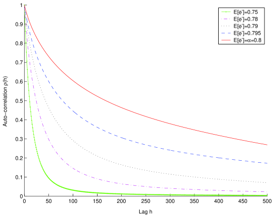
Figure 6: Auto-correlation function over 500 days for $p=5$, $q=0.75$, $\alpha=0.8$ and different values of $\bar{\varphi}^{\prime}$ ranging in $[0.60,0.79]$.

In the case $\bar{\varphi}^{\prime}\neq\alpha$, the condition for the denominator not to vanish becomes $\alpha>\max\left(\bar{\varphi}^{\prime},\frac{\left(1+\frac{q}{p-1}\right)\bar{\varphi}^{\prime}+2}{1-\frac{q}{p-1}}\right)$ if $\frac{q}{p-1}>1$ and $\bar{\varphi}^{\prime}<\alpha<\frac{\left(1+\frac{q}{p-1}\right)\bar{\varphi}^{\prime}+2}{1-\frac{q}{p-1}}$ if $\frac{q}{p-1}<1$. We set $p=5$, $q=0.75$ and $\alpha=0.8$. Figure 6 shows how the auto-correlation function behaves when $\bar{\varphi}^{\prime}$ tends to $\alpha$. We observe that the nearest $\bar{\varphi}^{\prime}$ is to $\alpha$ the slower the decrease of the auto-correlation function.

[Insert figure 6 about here]

As a special case, let us set $\alpha=1$, as in the case of rational agent, but $\bar{\varphi}^{\prime}\neq 0$. It is, in some sense, the simplest way to account for the departure from rationality. The anticipation of the agent $i$ then writes

$$\hat{X}_{i,t}=\varphi_{i}\cdot\left(\hat{X}_{i,t-1}-\bar{X}_{n,t-1}\right)+\bar{\varphi}^{\prime}\cdot\bar{X}_{n,t-1}+c_{i}\cdot\varepsilon_{t}+\eta_{i,t}\qquad t\geq 0,\qquad i=1,2,\dots,n,$$ (39)

which means that the agent performs her anticipation on the basis of the past innovation $\hat{X}_{i,t-1}-\bar{X}_{n,t-1}$ but, in addition, also pays attention to the past realized volatility in itself, as pointed out by the presence of the term $\bar{\varphi}^{\prime}\cdot\bar{X}_{n,t-1}$.

Equation (16) yields

$$\sum_{k=0}^{\infty}\tilde{\beta}_{k}x^{k}=\frac{1}{1-x\cdot\bar{\varphi}^{\prime}},$$ (40)

which shows that the dynamics of the (excess) realized log-volatility is nothing but a simple short memory AR(1) process

$$\bar{X}_{t}-\bar{\varphi}^{\prime}\cdot\bar{X}_{t-1}=\textrm{E}[c]\varepsilon_{t},$$ (41)

whose auto-correlation function is given by

$$\rho(h)=\bar{\varphi^{\prime}}^{|h|}$$ (42)

Thus, if $\bar{\varphi}^{\prime}=0$, the volatility exhibits exactly the same behavior as in the case of fully rational agents (case 1), which shows again that the rationality at the individual level is not a necessary condition for the volatility, at the aggregated level, to behave as if the agent were individually rational.

Long memory

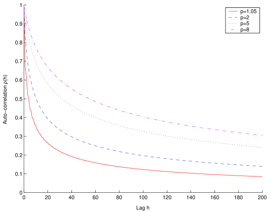
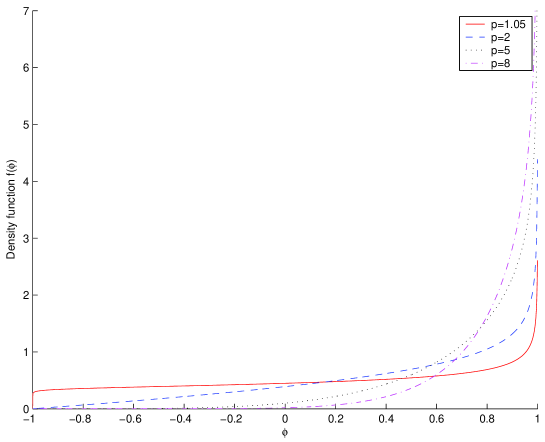
Figure 7: The left panel and the right panel represent respectively the auto-correlation function over 200 days and the density of the heterogeneous coefficient for $q=0.75$, $\alpha=0.3$ and different values of $p$ ranging in $[1.05,8]$. The law of $\varphi$ is a Beta($p$,$q$) extended over $[-1,1]$ and its density equal to $f(\varphi)=\frac{1}{2^{p+q-1}B(p,q)}(1+\varphi)^{p-1}(1-\varphi)^{q-1}$ explains the divergence near 0 and 1.

Let us now focus on the case where the model exhibits long memory, namely when $\bar{\varphi}^{\prime}=\alpha$. We are interested in the role of the parameters $p$, $q$ and $\alpha$ in the short and long memories. On figure 7, the role of $p$ is depicted. The two other parameters $q$ and $\alpha$ are fixed respectively to 0.75 and 0.3 and $p$ ranges between $1.05$ and $8$. On the left panel the auto-correlation functions are drawn over 200 lags, and on the right one the corresponding density functions. It shows that the larger $p$, the slower the decrease of the auto-correlation function at short lags. Thus, $p$ only influences the short term behavior of the auto-correlation function.

[Insert figure 7 about here]

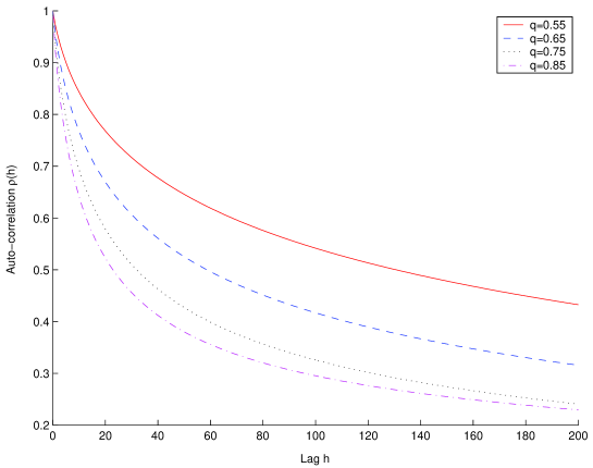
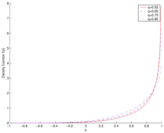
Figure 8: The left panel and the right panel represent respectively the auto-correlation function over 200 days and the density of the heterogeneous coefficient for $p=5$, $\alpha=0.3$ and different values of $q$ ranging in $[0.55,0.85]$. The law of $\varphi$ is a Beta($p$,$q$) extended over $[-1,1]$ and its density equal to $f(\varphi)=\frac{1}{2^{p+q-1}B(p,q)}(1+\varphi)^{p-1}(1-\varphi)^{q-1}$ explains the divergence near 0 and 1.

On figure 8, the role of $q$ is studied. The two other parameters $p$ and $\alpha$ are fixed respectively to 5 and 0.3 while $q$ ranges between $0.55$ and $0.85$. The closer $q$ is to 0.5, i.e. to the lower bound for second order stationarity, the faster is the divergence of the density function in the neighborhood of 1 and the slower is the decay of the auto-correlation function. Consequently, $q$ impacts on the long memory.

[Insert figure 8 about here]

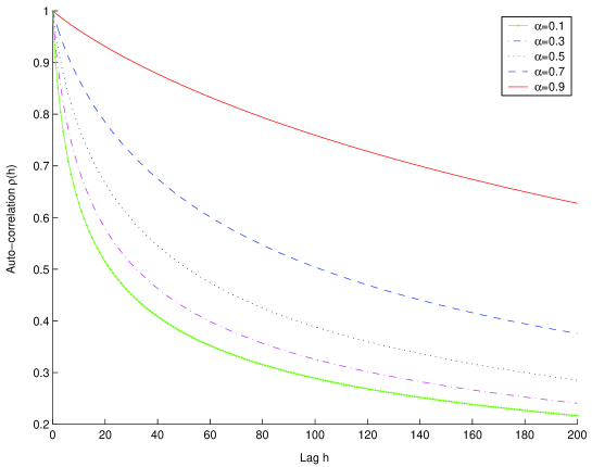
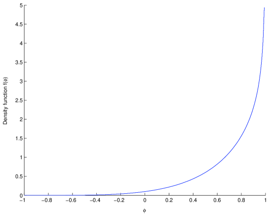
Figure 9: The left panel and the right panel represent respectively the auto-correlation function over 200 days and the density of the heterogeneous coefficient for $p=5$, $q=0.75$ and different values of $\alpha$ ranging in $[0.1,0.9]$. The law of $\varphi$ is a Beta($p$,$q$) extended over $[-1,1]$ and its density equal to $f(\varphi)=\frac{1}{2^{p+q-1}B(p,q)}(1+\varphi)^{p-1}(1-\varphi)^{q-1}$ explains the divergence near 0 and 1.

Figure 9 shows the role of $\alpha$. The two other parameters $p$ and $q$ are fixed respectively to 5 and 0.75 and $\alpha$ ranges betwwen $0.1$ and $0.9$. We observe that $\alpha$ has an important impact on the short memory. Indeed, the smaller $\alpha$, the slower the short-lag decrease.

[Insert figure 9 about here]

Let us take now into account a larger class of agents’ behavior in the case of $\bar{\varphi}^{\prime}=\alpha$. To this aim, we modify the density function: we still keep the beta law but we add another law which have a bell-like density. The bell will be able to move all over [-1,1]. For example, if the bell is set around zero, it means that the agents do not give importance to their past anticipation.

$$f(\varphi)=w\frac{1}{2^{p+q-1}B(p,q)}(1+\varphi)^{p-1}(1-\varphi)^{q-1}+(1-w)\frac{1}{K(m,\sigma)}(1+\varphi)(1-\varphi)\exp\left(-\frac{1}{2}\frac{(\varphi-m)^{2}}{\sigma^{2}}\right),$$ (43)

where $K$ is the normalizing constant (that can be expressed in closed-form) law and $w$ in $[0,1]$ is the weight given to the stretched Beta law.The conditions of long memory remain the same, only the conditions of stationarity change. They can be easily expressed in closed-form but their expression is rather cumbersome; That is why we will not give them here.

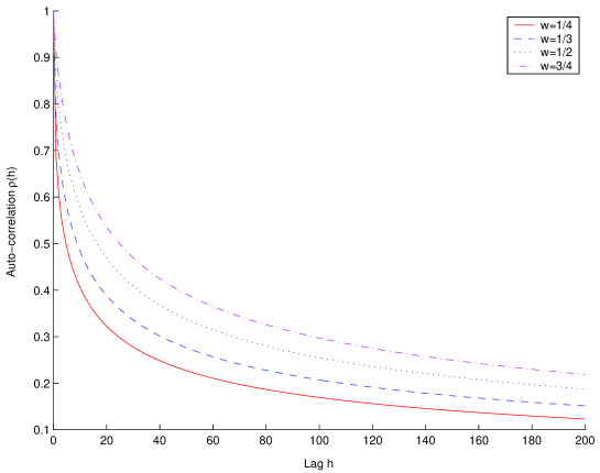
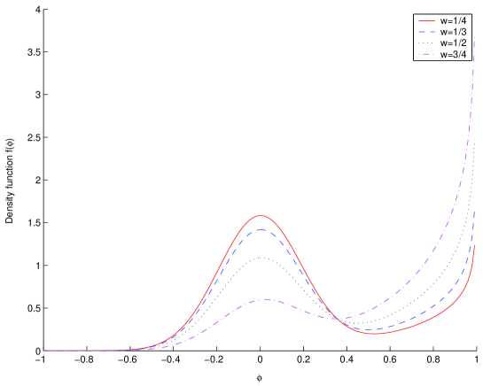
Figure 10: The left panel and the right panel represent respectively the auto-correlation function over 200 days and the density of the heterogeneous coefficient for $p=5$, $q=0.75$, $\alpha=0.3$, $m=0$, $\sigma=0.2$ and different values of $w$ ranging in $[1/4,3/4]$. The density of the law of $\varphi$ is equal to $f(\varphi)=w\frac{1}{2^{p+q-1}B(p,q)}(1+\varphi)^{p-1}(1-\varphi)^{q-1}+(1-w)\frac{1}{K}(1+\varphi)(1-\varphi)\exp\left(-\frac{1}{2}\frac{(\varphi-m)^{2}}{\sigma^{2}}\right)$ explains the divergence near 0 and 1.

On figure 10, the role of the relative weight of the singular part the density, $w$, is studied. The parameters $p$ and $q$ are fixed respectively to 5 and 0.75, $\alpha=0.3$, $m=0$, $\sigma=0.2$ and $w$ is ranged over $[1/4,3/4]$. The weight given to each density impacts on the short but not the long memory. The larger the relative part of the bell-like density compared to the stretched Beta one, the faster the decay of the short memory. In terms of agents’ behavior, it means that the more the agents base their anticipations on the incoming information flows and on the past realization of the volatility, the smallest the short-term correlations are.

[Insert figure 10 about here]

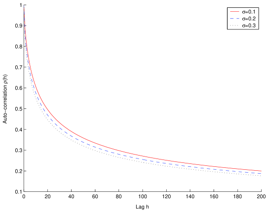
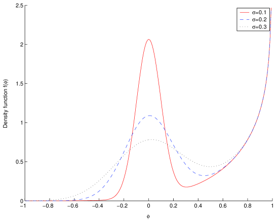
Figure 11: The left panel and the right panel represent respectively the auto-correlation function over 200 days and the density of the heterogeneous coefficient for $p=5$, $q=0.75$, $\alpha=0.3$, $m=0$, $w=1/2$ and different values of $\sigma$ ranging in $[0.1,0.3]$. The density of the law of $\varphi$ is equal to $f(\varphi)=w\frac{1}{2^{p+q-1}B(p,q)}(1+\varphi)^{p-1}(1-\varphi)^{q-1}+(1-w)\frac{1}{K}(1+\varphi)(1-\varphi)\exp\left(-\frac{1}{2}\frac{(\varphi-m)^{2}}{\sigma^{2}}\right)$ explains the divergence near 0 and 1.

Figure 11, shows the impact of the width of the peak of the bell controlled by $\sigma$. The parameters $p$ and $q$ are fixed respectively to 5 and 0.75, $\alpha=0.3$, $m=0$, $w=1/2$ and $\sigma$ ranges between $0.1$ and $0.3$. The intensity of the peak of the bell-like density has only a little impact on the short memory. The sharper the bell is, the more important is the short memory.

[Insert figure 11 about here]

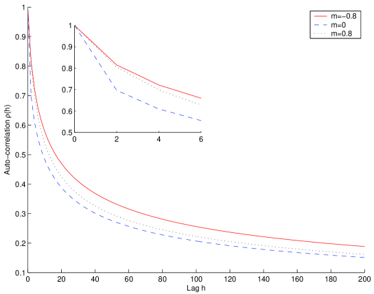
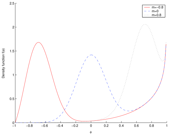
Figure 12: The left panel and the right panel represent respectively the auto-correlation function over 200 days and the density of the heterogeneous coefficient for $p=5$, $q=0.75$, $\alpha=0.3$, $\sigma=0.2$, $w=1/3$ and different values of $m$ ranging in $[-0.8,0.8]$. The density of the law of $\varphi$ is equal to $f(\varphi)=w\frac{1}{2^{p+q-1}B(p,q)}(1+\varphi)^{p-1}(1-\varphi)^{q-1}+(1-w)\frac{1}{K}(1+\varphi)(1-\varphi)\exp\left(-\frac{1}{2}\frac{(\varphi-m)^{2}}{\sigma^{2}}\right)$ explains the divergence near 0 and 1.

On figure 12, the role of $m$ which determines the position of the bell is studied. The parameters $p$ and $q$ are fixed respectively to 5 and 0.75, $\alpha=0.3$, $\sigma=0.2$, $w=1/3$ and $m$ is ranged over $[-0.8,0.8]$. The translation of the bell plays a part on short memory. Over the very first lags, we notice that the closer the bell is to -1, the faster the decrease of the auto-correlation function is. But after a few lags, this situation does not hold anymore.

[Insert figure 12 about here]

3 Statistical Inference

Let us now turn to the question of the estimation of the parameters of the model. As exemplified in the previous section, the long memory phenomenon can be ascribed to the hyperbolic divergence of the density of the heterogeneity parameter $\varphi$ in the neighborhood of $1^{-}$. It is thus convenient to split the density of the heterogeneity variable $\varphi$ in two terms: a regular one and a singular one. For this reason, we will model the law of the realized log-volatility of financial assets as the mixture of a regular law, with density $f_{1}$, and of a Beta$(2,1-d)$ law ($d\in]0;1[$) with density $f_{2}$, that will allow capturing the hyperbolic divergence of the density of $\varphi$ at one. As a consequence, the density of $\varphi$ can be written as

$$f(x)=wf_{1}(x)+(1-w)f_{2}(x),\quad w\in[0,1],$$ (44)

where $f_{1}$ is any regular, i.e. continuous and bounded, density function defined on $[-1,1]$ and

$$f_{2}(x)=(1-d)(2-d)\frac{x}{(1-x)^{d}}1_{[0;1]}(x).$$ (45)

Given a density $f_{1}(x)$ which admits an expansion in terms of a Fourier series, an assumption that will be made in all the sequel of this article,

$$f_{1}(x)=\frac{1}{2}+\sum_{n=1}^{\infty}a_{n}\cos(n\pi x)+\sum_{n=1}^{\infty}b_{n}\sin(n\pi x),\quad x\in[-1,1],$$ (46)

the expression of the auto-covariance and auto-correlation functions of the realized log-volatility can be numerically calculated by use of the expression of the moment of order $k$ of the heterogeneity variable $\varphi$

$$\textrm{E}\left[\varphi^{k}\right]=w\textrm{E}_{1}\left[\varphi^{k}\right]+(1-w)\textrm{E}_{2}\left[\varphi^{k}\right],$$ (47)

where $\textrm{E}_{1}[\cdot]$ and $\textrm{E}_{2}[\cdot]$ denotes the expectations with respect to $f_{1}$ and $f_{2}$ respectively, which yields

$$\textrm{E}\left[\varphi^{k}\right]=w\left(\frac{1}{2}A_{k}+\sum_{n=1}^{\infty}a_{n}B_{n,k}+\sum_{n=1}^{\infty}b_{n}C_{n,k}\right)+(1-w)\cdot\frac{\Gamma(k+2)}{\Gamma(k+3-d)}\Gamma(3-d),$$ (48)

where the expressions of $A_{k}$, $B_{k}$ and $C_{k}$ are given in appendix D.

3.1 Asymptotic Normality of the estimator

For simplicity, and for ease of the exposition, we will assume that the coefficients $(a_{n},b_{n})$ of the Fourier expansion (46) vanishes beyond the rank $q$, so that the density $f_{1}$ reads

$$f_{1}(x)=\frac{1}{2}+\sum_{n=1}^{q}a_{n}\cos(n\pi x)+\sum_{n=1}^{q}b_{n}\sin(n\pi x),\quad x\in[-1,1].$$ (49)

In addition, we focus on the case where $\textrm{E}\left[\psi|\varphi\right]=-\alpha(\varphi-1)$, which ensures that the long range memory of the volatility is controlled by the parameter $d$ of the Beta law, as shown in the previous section.

Let us denote by $\theta=(a_{1},\dots,a_{q},b_{1},\ldots,b_{q},\alpha,w,\sigma_{\varepsilon},d)^{\prime}$ the $2q+4$ dimensional vector of the parameters involved in our problem and by $\gamma(h;\theta)$ the value of the auto-covariance function at lag $h$ for the distribution of heterogeneity defined by equations (44), (45) and (49) and for the parameter value $\theta$.

Given the $T$-sample of the logarithm of the realized volatilities $\{\omega_{1},\dots,\omega_{T}\}$, treated as observed data, it seems natural to estimate $\theta$ by minimization of the weighted difference between the sample auto-covariance function

$$\hat{\gamma}_{T}(h)=\frac{1}{T}\sum_{i=1}^{T-h}\left(\omega_{i}-\bar{\omega}_{T}\right)\left(\omega_{i+h}-\bar{\omega}_{T}\right),\qquad h=0,1,\dots$$ (50)

and $\gamma(h;\theta)$, the auto-covariance function at the parameter value $\theta$. We could thus consider the classical minimum distance estimator $\hat{\theta}_{T,L}$ [newey94] solution to

$$\min_{\theta\in\Theta}\left[\hat{\gamma}_{T,L}-\gamma_{L}(\theta)\right]^{\prime}W_{L}^{-1}\left[\hat{\gamma}_{T,L}-\gamma_{L}(\theta)\right],$$ (51)

where $\gamma_{L}(\theta)=\left(\gamma(1;\theta),\dots,\gamma(L;\theta)\right)^{\prime}$, $\hat{\gamma}_{T,L}=\left(\hat{\gamma}_{T}(1),\dots,\hat{\gamma}_{T}(L)\right)^{\prime}$ and $W_{L}$ is any symmetric positive definite $L\times L$ matrix, while $\Theta$ is the parameter set

$$\Theta=\left\{\theta=(a_{1},\dots,a_{q},b_{1},\ldots,b_{q},\alpha,w,\sigma,d)^{\prime};~{}f_{1}\geq 0,~{}0<d<1~{}\text{and}~{}0\leq w\leq 1\right\}.$$ (52)

However, when dealing with long-memory time series, i.e such that $\sum_{h=0}^{\infty}|\gamma(h)|=\infty$, the asymptotic properties of the sample estimates $\hat{\gamma}_{T,L}$ are not really suitable. Indeed, as recalled by hosking96, the limiting distribution of $\gamma_{T}(h)$ when $d>0$ is such that

$$T^{1-2d}\left(\hat{\gamma}_{T}(h)-\gamma(h)\right)\stackrel{{\scriptstyle{\cal L}}}{{\longrightarrow}}{\cal R},$$ (53)

where ${\cal R}$ denotes the modified Rosenblatt distribution. In particular, the mean of the Rosenblatt distribution is not equal to zero and can even be much larger than its standard deviation for $d$ larger than or of the order of one fourth.

As a consequence, it is desirable to rely on the minimization of another criteria with more suitable asymptotic properties. In fact, irrespective of the value of $d\in(-\frac{1}{2},\frac{1}{2})$, the limit distribution of any subset of the variables $D_{h}=\sqrt{T}\left[\left(\hat{\gamma}_{T}(h)-\hat{\gamma}_{T}(0)\right)-\left(\gamma(h)-\gamma(0)\right)\right]$, $h\geq 1$ is a multivariate normal with zero mean and asymptotic covariance matrix (see [th. 5]hosking96)

$$\left[\Sigma^{2}\right]_{kl} = \lim_{T\rightarrow\infty}{\rm Cov}\left(D_{k},D_{l}\right),$$ (54)

$$= \frac{1}{2}\sum_{s=-\infty}^{\infty}\left[\gamma(s)-\gamma(s-k)-\gamma(s-l)+\gamma(s-k+l)\right]^{2}.$$ (55)

In view of this asymptotic result, a convenient estimator of the parameter $\theta$ is given by the solution to

$$\min_{\theta\in\Theta}\left[\hat{\eta}_{T,L}-\eta_{L}(\theta)\right]^{\prime}W_{L}^{-1}\left[\hat{\eta}_{T,L}-\eta_{L}(\theta)\right],$$ (56)

where

$$\eta_{L}(\theta)=\left(\gamma(1;\theta)-\gamma(0;\theta),\dots,\gamma(L;\theta)-\gamma(0;\theta)\right)^{\prime},$$ (57)

and

$$\quad\hat{\gamma}_{T,L}=\left(\hat{\gamma}_{T}(1)-\hat{\gamma}_{T}(0),\dots,\hat{\gamma}_{T}(L)-\hat{\gamma}_{T}(0)\right)^{\prime}.$$ (58)

The consistency and the asymptotic normality of the estimator $\hat{\theta}_{T,L}$ follows from the general asymptotic properties of the classical minimum distance estimators. Concerning the asymptotic normality, we can state the following result

Proposition 3.

Assuming that $\theta_{T,L}\stackrel{{\scriptstyle P}}{{\longrightarrow}}\theta_{0}$, for all $L\geq 2q+4$, as $T\longrightarrow\infty$,

$$\sqrt{T}\left(\hat{\theta}_{T,L}-\theta_{0}\right)\stackrel{{\scriptstyle{\cal L}}}{{\longrightarrow}}{\cal N}\left(0,A_{L}(\theta_{0})\right),$$ (59)

with

$$A_{L}(\theta_{0})=\left[G_{L}(\theta_{0})^{\prime}W_{L}G_{L}(\theta_{0})\right]^{-1}G_{L}(\theta_{0})^{\prime}W_{L}\Sigma_{L}^{2}(\theta_{0})W_{L}G_{L}(\theta_{0})\left[G_{L}(\theta_{0})^{\prime}W_{L}G_{L}(\theta_{0})\right]^{-1},$$ (60)

where

$$G_{L}(\theta_{0})=\left.{\rm grad}_{\theta}\eta_{L}(\theta)\right|_{\theta=\theta_{0}},$$ (61)

and

$$\left[\Sigma_{L}^{2}(\theta_{0})\right]_{lk}=\frac{1}{2}\sum_{s=-\infty}^{\infty}\left[\gamma\left(s;\theta_{0}\right)-\gamma\left(s-k;\theta_{0}\right)-\gamma\left(s-l;\theta_{0}\right)+\gamma\left(s-k+l;\theta_{0}\right)\right]^{2},$$ (62)

$l,k=1,\dots,L$.

Proof.

By theorem 5 in hosking96, $\displaystyle\sqrt{T}\left(\hat{\eta}_{T,L}-\eta_{L}(\theta_{0})\right)\stackrel{{\scriptstyle{\cal L}}}{{\longrightarrow}}{\cal N}\left(0,\Sigma_{L}^{2}(\theta_{0})\right)$, thus, the result follows straightforwardly from theorem 3.2 in newey94. ∎

For fixed $L$, the minimum of the asymptotic variance $A_{L}(\theta_{0})$ is reached when $W_{L}=\left[\Sigma_{L}^{2}(\theta_{0})\right]^{-1}$, so that

$$\sqrt{T}\left(\hat{\theta}_{T,L}-\theta_{0}\right)\stackrel{{\scriptstyle{\cal L}}}{{\longrightarrow}}{\cal N}\left(0,G_{L}(\theta_{0})^{\prime}\left[\Sigma_{L}^{2}(\theta_{0})\right]^{-1}G_{L}(\theta_{0})\right).$$ (63)

On the other hand, given $W_{L}$, one can get an optimal value $L^{*}$ of $L$ as the solution to

$$L^{*}=\arg\min_{L\in\{2q+4,\dots,T-1\}}||A_{L}(\theta_{0})||^{2}.$$ (64)

Proposition 4.

Under the assumptions in proposition 3, denoting by $D(\theta)$ the vector

$$D(\theta)=\left[\begin{array}[]{c}w\cos(\pi x)\\ \vdots\\ w\cos(q\pi x)\\ w\sin(\pi x)\\ \vdots\\ w\sin(q\pi x)\\ 0\\ f_{1}(x)-f_{2}(x)\\ 0\\ (w-1)f_{2}(x)\left[\ln(1-x)+\frac{3-2d}{(1-d)(2-d)}\right]\end{array}\right],$$ (65)

the estimator $\hat{f}(x)$ of the density $f(x)$ is asymptotically Gaussian

$$\sqrt{T}\left(\hat{f}(x)-f(x)\right)\stackrel{{\scriptstyle{\cal L}}}{{\longrightarrow}}{\cal N}\left(0,D(\theta_{0})^{\prime}A(\theta_{0})D(\theta_{0})\right).$$ (66)

Proof.

$D(\theta)$ is nothing but the gradient of $f(x)$ with respect to $\theta$. Thus, by use of the Delta method [vaart00], the result follows straightforwardly from proposition 3. ∎

4 Empirical results

In this section we present the conclusions drawn from the calibration of our model whose implementation is discussed in appendix E. To this aim, we use the intraday prices of ten middle and fourteen large capitalization stocks traded on the NYSE or the Nasdaq from 01/01/1994 to 12/31/2003 (which represents 2518 trading days). The description of the data, provided by TickData, is given in table 1.

[Insert table 1 about here]

We first estimate the daily realized-volatility by use of the estimator (1), as already discussed in section 1. We stress that this variable will be considered as an observed variable in all the sequel. Before going further, it is worth to notice that we should get 390 one-minute prices for all assets since the quotations begin at 9:30 am and end at 16:00 pm. However, we have much less observations for the middle capitalization stocks than expected: typically 133 per day, on average. In addition, the number of intraday quotations is not constant over time. Indeed, the number of available data is much smaller from 1994 to 1997 than from 1998 to 2003 (respectively 45 and 192 for the middle capitalizations and 282 and 374 for the large capitalizations). Nevertheless, we has chosen to estimate the realized volatility over the whole time period ranging from 01/01/1994 to 12/31/2003.

4.1 Calibration of the model over the whole time interval

Let us underline that the estimation of the density of the heterogeneity variable $\varphi$ provides us access to the parameter $d$ that characterizes the long-memory behavior of the time series of the realized log-volatility. It is then interesting to compare the values of $d$ obtained with our model and those obtained by other methods like the rescaled rang method set by hurst51 and the regression method introduced geweke83. Notice that the former method has been refined by mandelbrot72 mandelbrot72,mandelbrot75, mandelbrot79 and later by lo91. However, his generalization involves an additional parameter whose value has a great influence on the results [teverovsky99]. As a consequence, we have only resorted to the classical rescaled range statistic.

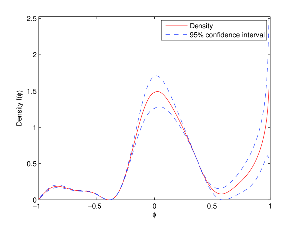
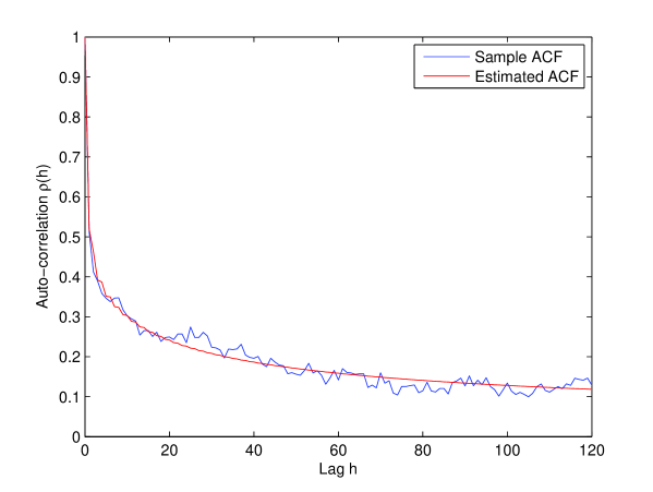
Figure 13: Estimation of the density with its 95 % confidence interval (on the left panel) and the auto-correlation function from lag 0 to lag 120 (on the right panel) for FNF.

First we show the graphical results obtained for a middle capitalization: Fidelity National Financial inc. (FNF, see figure 13). On the right panel the estimated auto-correlation function fits very well the sample one. The density of the heterogeneity variable $\varphi$ is depicted on the left panel (plain curve) with the pointwise 95% confidence interval (dashed curves). This shape with three distinct masses (one close to -1, an other close to 1 and the last one around 0) is representative of half of the assets (The other half is depicted afterwards). In terms of agents’ behavior, it means that there is mainly three kinds of agents. First, looking at the central part of the density function, we can conclude that most of the agents base their anticipations on the incoming flow of information and on the past realization (depending on the value of $\alpha$). Some others believe in the anticipation they performed the day before, which is related to the diverging part of the curve, in the neighborhood of one, while only a few, shown by the part of the density near -1, systematically take the opposite of their previous anticipations.

[Insert figure 13 about here]

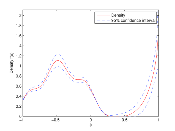
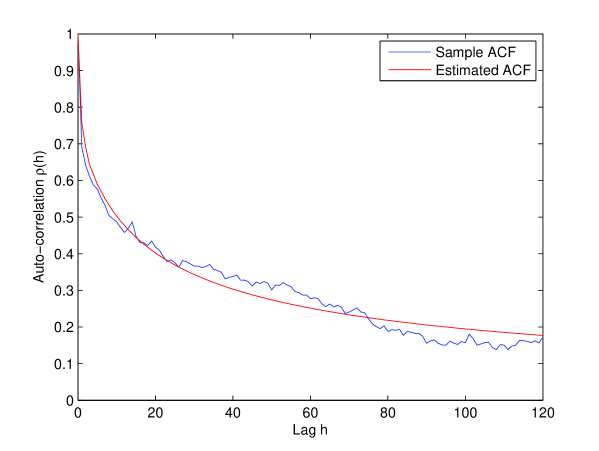
Figure 14: Estimation of the density with its 95 % confidence interval (on the left panel) and the auto-correlation function from lag 0 to lag 120 (on the right panel) for Microsoft.

Secondly we show what we graphically obtain for the other half of the assets with the example of a large capitalization: Microsoft (MSFT, see figure 14). Instead of noticing three distinct masses, we only see two. The agents confident in their past anticipation still remains, but it is now more vague with the second category. In fact the curve is symmetric with a peak centered around -0.5. We still find agents who do not trust anymore in the anticipation they performed the previous day (the part of the density function near -1), and others who only care about incoming news (the part of the density function near 0), and between these two situations there are many agents who both take into account the news and the opposite of their past anticipation. This is quite logical if an agent realizes that her past anticipation was far from the realization of the volatility, then she takes the opposite of her previous anticipation and also becomes more careful in the incoming news.

[Insert figure 14 about here]

These two typical shapes of the distribution of heterogeneity does not appear to be related to the size of the firms nor to any specific industry. However, the small number of assets per industry in our database (maximum five) prevents us from drawing definitive conclusions.

The results of the estimations of the long memory parameter $d$ by our model and by the two semi-parametric methods are shown in table 2. It is quite obvious that, on the one hand, each estimators agrees to say that long memory is present in almost all series while, on the other hand, each estimator gives, for a same asset, different values of $d$. Most of the values obtained by our model range between $0.2$ and $0.4$ and a few are negative, instead of between $0.3$ and $0.45$ with Geweke and Porter-Hudak’s estimator. At least the long memory parameter obtained by the classical rescaled range analysis method is mainly contained between $0.40$ and $0.55$.

It is common knowledge that beyond $d=0.5$ the series is no longer stationary. As the estimations by the Hurst method are greater than, but close to, 0.5, we may say that it is due to the uncertainty and, maybe, the inaccuracy of the method. Moreover, the differences noticed between these results may be explained by the difficulty to use the estimators. Indeed, it is well-known that Geweke and Porter-Hudak’s estimator is quite sensitive to the presence of short memory. On the contrary, our estimates should be considered as more robust vis-a-vis the presence of short-memory insofar as our model takes it into account explicitly.

4.2 Study of the bubble burst effect

The study of the bubble burst effect is motivated by the fact that we will be able to get informations about the agents’ behavior during a prosperity period (before the bubble burst) and during a recession period (after the bubble burst). In particular we will be able to answer the question:“Do the agents behave differently before and after a bubble burst ?”

To perform the computations, we randomly selected 5 large capitalizations because the bubble phenomenon is far more pronounced in their price evolution than it is for middle capitalizations. We simply split the series when the maximum price is reached into two subseries. The first one is defined as the pre-bubble burst period while the other one is the post-bubble burst period. Hereafter, the illustrations are drawn for a “new technology” company, Cisco Systems (CSCO), and a distribution company, Coca Cola (KO). The point is that the bubble phenomenon may be more pronounced in the price evolution of a new technology company, which was more affected by the internet bubble, than a non technology firm.

4.2.1 Study of a new technology asset: Cisco Systems

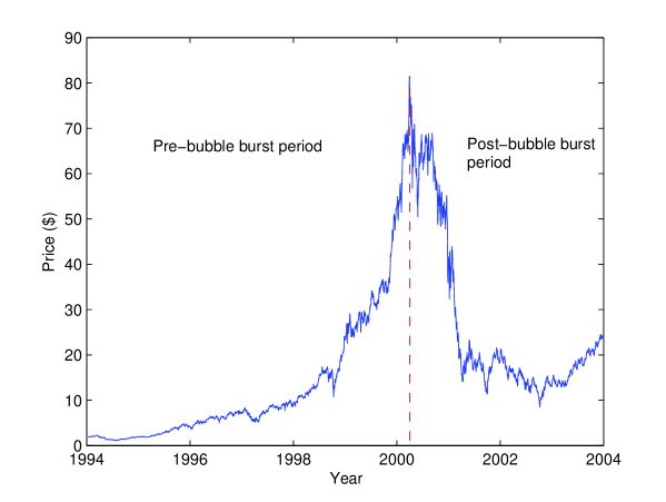
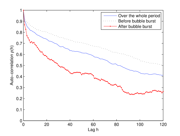
Figure 15: On the left panel is presented the evolution of the price of Cisco Systems over the period considered in order to study the bubble burst effect. On the right panel, the auto-correlations over different periods are drawn.

On the left panel of figure 15 we show the price evolution of CSCO between 01/01/1994 and 12/31/2003. On the right panel of figure 15 we have drawn the sample auto-correlation functions of CSCO over the three periods. From it we easily deduce that on the one hand before the bubble burst the long memory parameter may be much larger than the one over the whole period, and on the other hand after the bubble burst, it must be a lot smaller.

[Insert figure 15 about here]

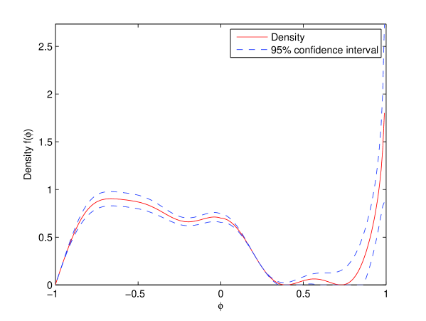
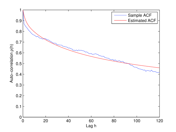
Figure 16: Density of the heterogeneity coefficient (on the left) and auto-correlation of the realized log-volatility of Cisco Systems (on the right) over the pre-bubble burst period.

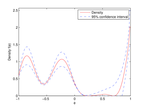
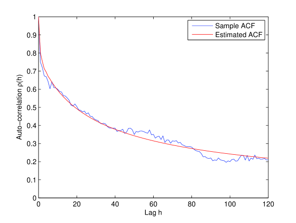
Figure 17: Density of the heterogeneity coefficient (on the left) and auto-correlation of the realized log-volatility of Cisco Systems (on the right) over the post-bubble burst period.

Let us complete these impressions with the densities and auto-correlation functions estimated over the two subperiods (see figures 16 and 17). We show on the left panel the estimated density with its 95% confidence interval and on the right one the sample and estimated auto-correlation functions.

Concerning the pre-bubble burst period (see figure 16), on the right side, we see that the estimated auto-correlation function fits pretty well to the sample one. Moreover on the left side of this figure, the 95% confident interval is very thin. We deduce that the optimization performed well.

The shape of the density is quite similar as the one we obtained with Microsoft (see figure 14) and implies a strong long memory. To sum up, we get two masses: the one close to 1 represents agents who believe in their past anticipation; the other one, from -1 to 0.2 includes several different behaviors. Nevertheless they have something in common: they do not replicate their past anticipation. Some are rational and use the incoming information flows and others not really. They are inspired by the opposite of their past anticipation or a mix between the news and the contrary of the previous anticipation.

[Insert figure 16 about here]

As for the post-bubble burst period, we first notice on figure 17 that the estimated auto-correlation function fits very well to the sample one (on the right panel) and that the 95% confident interval of the density function is good too.

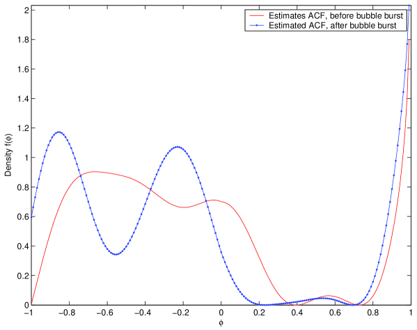
Figure 18: Pre bubble burst density compared to post bubble burst density of Cisco Systems.

Here, the situation is a little bit different: the value of the long memory parameter $d$ is smaller (see table 3 hereafter). Basically, it means that the proportion of agents who believe in the continuity of the previous market conditions is smaller. Figure 18 helps us compare the agents behaviors during the two subperiods. We observe that after the bubble burst the mass from -1 and 0.2 changes. It was first compressed between -1 and 0, then the mass has got divided into two masses. As a consequence, on the one hand the proportion of agents who perform their anticipation basing their judgment on the contrary to their previous anticipation is greater. Those agents may recognize that they were wrong or it can reflect the confusion resulting from the increase in the level of uncertainty about the future evolution of the economic environment after the bubble burst. On the other hand, the proportion of agents who mainly use information is greater too, in accordance with the increase in the level of uncertainty and therefore with the increasing need for information.

[Insert figure 17 about here]

[Insert figure 18 about here]

4.2.2 Study of a non technology asset : Coca Cola

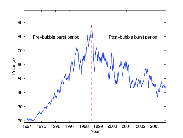
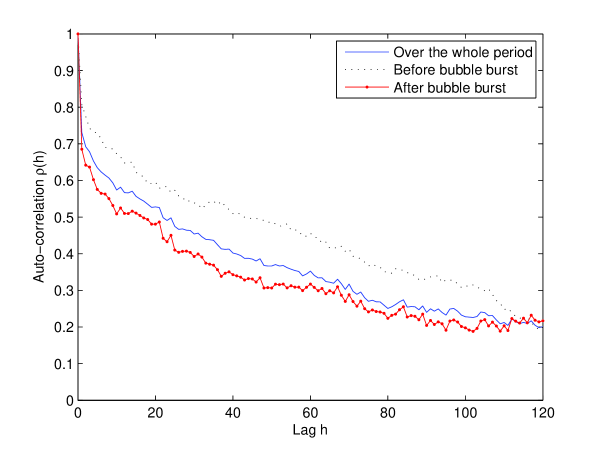
Figure 19: On the left panel is presented the evolution of the price of Coca Cola over the period considered in order to study the bubble burst effect. On the right panel, the auto-correlations over different periods are drawn.

We reproduce for Coca Cola the same figures as for Cisco Systems. We notice on the left side of figure 19 that the bubble phenomenon is less obvious as observed previously. The immediate consequence is shown on the left side of this figure where the sample auto-correlation functions over the three periods are not as different as they are for CSCO. Then we expect to get closer long memory parameters, especially over the whole period and after the bubble burst.

[Insert figure 19 about here]

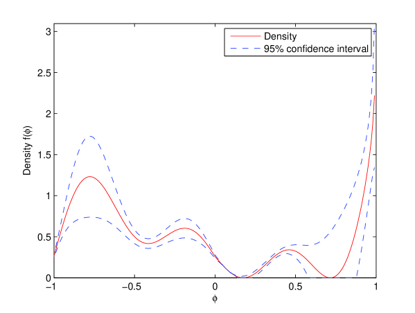
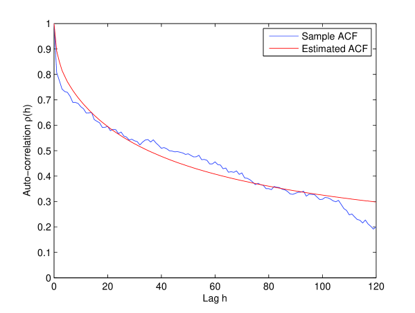
Figure 20: Density of the heterogeneity coefficient (on the left) and auto-correlation of the realized log-volatility of Coca Cola (on the right) over the pre-bubble burst period.

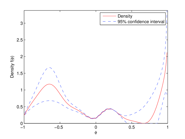
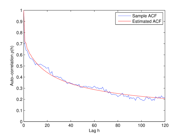
Figure 21: Density of the heterogeneity coefficient (on the left) and auto-correlation of the realized log-volatility of Coca Cola (on the right) over the post-bubble burst period.

Let us be more accurate with the densities and auto-correlation functions estimated over the two subperiods (see figures 20 and 21). For both of the figures, notice that the estimated auto-correlation functions on the right panels fit very well to the sample ones (in particular after the burst), and the 95% confident intervals are good too.

[Insert figure 20 about here]

[Insert figure 21 about here]

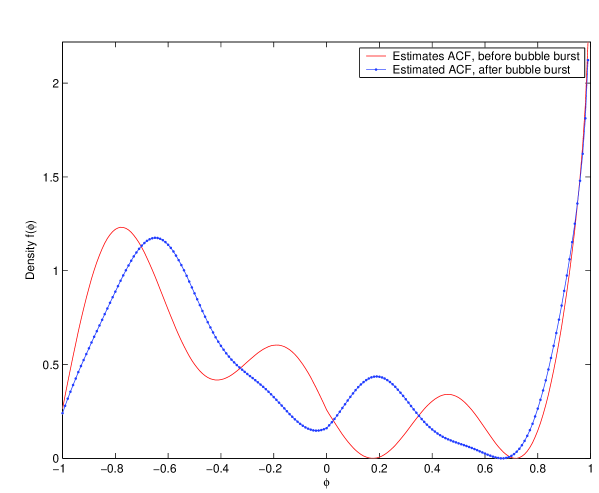
Figure 22: Pre bubble burst density compared to post bubble burst density of Coca Cola.

As the shapes of these two densities look very similar let us put them together on the same graphic in order to analyze them (see figure 22). Looking at the divergence at one, the long memory parameter may be more or less the same. Contrary to the evolution of CSCO density where the bulk of the post bubble burst density in the negative range was compressed, here it does not change that much. It only slightly expands along the positive axis after the bubble burst. The mass from 0.2 to 0.7 for the pre-bubble burst period which represent the agents who both believe in the continuity of the market and also take into account the information flows has disappeared. It means that a smaller fraction of agents still use their past anticipation.

[Insert figure 22 about here]

4.2.3 General observations

Let us look at the values of $d$. The values of the long memory parameter obtained by our model (see table 3) confirm our visual impressions. Indeed, before the burst, the long memory parameter is often greater than the one over the whole period for 4 out of 5 cases (in the 5th they are nearly similar). On the opposite, one observes that after the burst, $d$ falls for all the assets except for Coca Cola.

We have to mention that the very large standard deviation of the $d$-estimate for Microsoft during the second period should raise doubts about the convergence of our algorithm in this case. A reason might be the small number of available data. Indeed, for the post bubble burst period we only have about 900 days for 4 out of 5 assets whereas we have about 1600 data available for the pre bubble burst period. In the case of a smaller data number, the global optimum is more difficult to reach. Consequently the result may be wrong.

Nonetheless, to sum up, the results we obtained lead us to conclude that during a growth cycle, the number of agents who are confident in the market and whose strategy remains almost the same day after day, is greater than the one during a decline cycle where the agents adopt more various behaviors. Indeed, some still base their anticipation on the previous one. Some do not believe in their past anticipation anymore and take into account the information flow. Some admit they were wrong the day before and make a contrary anticipation. Others make a mix between a contrary anticipation and taking into account the news.

5 Conclusion

Based upon the recent literature on the aggregation theory, we have provided a model of realized log-volatility that aims at relating the behavior of the economic agents to the long memory of the volatility of asset returns. In spite of its simplicity, this model allows taking into account many agents’ behavior and performs good estimates in general. The estimated coefficients often lead to auto-covariance and auto-correlation functions well fitted with their sample counterparts. In addition, the results derived from the study of the bubble burst effect – namely a higher tendency to replicate the anticipations of the day before and to neglect the incoming information flow before the bubble burst than after – are quite reasonable.

Appendix A Proof of proposition 1

Under the assumption $||A||<1$, the stationary solution of equation (12) is given by

$$\hat{X}_{t}=\sum_{k=0}^{\infty}A^{k}C\varepsilon_{t-k}+\sum_{k=0}^{\infty}A^{k}\eta_{t-k},$$ (67)

and the excess realized log-volatility writes

$$\bar{X}_{n,t}=\sum_{k=0}^{\infty}\left(\frac{1}{n}1_{n}^{\prime}A^{k}C\right)\varepsilon_{t-k}+\sum_{k=0}^{\infty}\frac{1}{n}1_{n}^{\prime}A^{k}\eta_{t-k}.$$ (68)

Accounting for the fact $A=D+\frac{1}{n}\Psi\cdot 1_{n}^{\prime}$, $A^{k}$ is solution of

$$A^{k}=A^{k-1}\left(D+\frac{1}{n}\Psi\cdot 1_{n}^{\prime}\right),$$ (69)

so that one has to solve the recurrence equation

$$1_{n}^{\prime}A^{k}=\left(1_{n}^{\prime}A^{k-1}\right)D+\beta_{k-1}1_{n}^{\prime},$$ (70)

where $\beta_{k}=\frac{1}{n}1_{n}A^{k}\psi$. It is then a matter of simple algebraic manipulations to show that

$$\frac{1}{n}1_{n}^{\prime}A^{k}C = \frac{1}{n}1_{n}^{\prime}D^{k}C+\frac{1}{n}\sum_{i=1}^{k}\beta_{i-1}\cdot 1_{n}^{\prime}D^{k-i}C,$$ (71)

$$= \textrm{E}\left[c\right]\cdot\textrm{E}\left[\varphi^{k}\right]+\textrm{E}\left[c\right]\sum_{i=1}^{k}\beta_{i-1}\textrm{E}\left[\varphi^{k-i}\right]\quad{\rm(a.s)},\qquad{\rm as}~{}n\rightarrow\infty,$$ (72)

where

$$\beta_{k} = \frac{1}{n}1_{n}^{\prime}D^{k}\Psi+\sum_{i=1}^{k}\beta_{i-1}\cdot\left(\frac{1}{n}1_{n}^{\prime}D^{k-i}\Psi\right),$$ (73)

$$= \textrm{E}\left[\psi\varphi^{k}\right]+\sum_{i=1}^{k}\beta_{i-1}\cdot\textrm{E}\left[\psi\varphi^{k-i}\right]\quad{\rm(a.s)},\qquad{\rm as}~{}n\rightarrow\infty,$$ (74)

while

$$\frac{1}{n}1_{n}^{\prime}A^{k}\eta_{t_{k}} = \frac{1}{n}1_{n}^{\prime}D^{k}\eta_{t_{k}}+\frac{1}{n}\sum_{i=1}^{k}\beta_{i-1}\cdot 1_{n}^{\prime}D^{k-i}\eta_{t_{k}},$$ (75)

$$= \textrm{E}\left[\varphi^{k}\right]\textrm{E}\left[\eta_{t}\right]+\sum_{i=1}^{k}\beta_{i-1}\textrm{E}\left[\varphi^{k-i}\right]\textrm{E}\left[\eta_{t}\right]\quad{\rm(a.s)},\qquad{\rm as}~{}n\rightarrow\infty,$$ (76)

$$= 0,$$ (77)

provided that $\textrm{E}\left[\eta_{t}\right]=0$.

So, $\bar{X}_{t}=\lim_{n\rightarrow\infty}\bar{X}_{n,t}$ is equal to

$$\bar{X}_{t}=\textrm{E}\left[c\right]\cdot\sum_{k=0}^{\infty}\left(\textrm{E}\left[\varphi^{k}\right]+\sum_{i=1}^{k}\beta_{i-1}\textrm{E}\left[\varphi^{k-i}\right]\right)\varepsilon_{t-k}.$$ (78)

Let us simplify this expression by setting

$$\tilde{\beta}_{k}=\textrm{E}\left[\varphi^{k}\right]+\sum_{i=1}^{k}\beta_{i-1}\textrm{E}\left[\varphi^{k-i}\right],$$ (79)

so that

$$\bar{X}_{t}=\textrm{E}\left[c\right]\cdot\sum_{k=0}^{\infty}\tilde{\beta}_{k}\varepsilon_{t-k}.$$ (80)

Now, multiplying equation (79) by $x^{k}$ and summing over $k$ from zero to infinity, we get

$$\sum_{k=0}^{\infty}\tilde{\beta}_{k+1}x^{k+1}=\sum_{k=0}^{\infty}\textrm{E}\left[\varphi^{k+1}\right]x^{k+1}+\sum_{k=0}^{\infty}\left(\sum_{i=0}^{k}\beta_{i}\textrm{E}\left[\varphi^{k-i}\right]\right)x^{k+1}.$$ (81)

As it is well-known that

$$\sum_{k=0}^{\infty}\left(\sum_{i=0}^{k}\beta_{i}\textrm{E}\left[\varphi^{k-i}\right]\right)x^{k+1}=x\left(\sum_{k=0}^{\infty}\beta_{k+1}x^{k}\right)\left(\sum_{k=0}^{\infty}\textrm{E}\left[\varphi^{k}\right]x^{k}\right),$$ (82)

we obtain

$$\sum_{k=0}^{\infty}\tilde{\beta}_{k}x^{k}=\sum_{k=0}^{\infty}\textrm{E}\left[\varphi^{k}\right]x^{k}\left\{1+x\sum_{k=0}^{\infty}\beta_{k}x^{k}\right\}.$$ (83)

Then, focusing on $\displaystyle\sum_{k=0}^{\infty}\beta_{k}x^{k}$ and by use of equation (74), the same argument yields

$$\sum_{k=0}^{\infty}\beta_{k+1}x^{k+1}=\sum_{k=0}^{\infty}\textrm{E}\left[\psi\varphi^{k+1}\right]x^{k+1}+\sum_{k=0}^{\infty}\left(\sum_{i=0}^{k}\beta_{i}\textrm{E}\left[\psi\varphi^{k-i}\right]\right)x^{k+1},$$ (84)

$$\sum_{k=0}^{\infty}\beta_{k}x^{k}=\sum_{k=0}^{\infty}\textrm{E}\left[\psi\varphi^{k}\right]x^{k}+x\left(\sum_{i=0}^{\infty}\beta_{i}x^{i}\right)\left(\sum_{i=0}^{\infty}\textrm{E}\left[\psi\varphi^{i}\right]x^{i}\right).$$ (85)

In other words

$$\sum_{k=0}^{\infty}\beta_{k}x^{k}=\frac{\displaystyle\sum_{k=0}^{\infty}\textrm{E}\left[\psi\varphi^{k}\right]x^{k}}{\displaystyle 1-x\sum_{k=0}^{\infty}\textrm{E}\left[\psi\varphi^{k}\right]x^{k}},$$ (86)

which, by replacement in equation (83), leads to

$$\sum_{k=0}^{\infty}\tilde{\beta}_{k}x^{k}=\frac{\displaystyle\sum_{k=0}^{\infty}\textrm{E}\left[\varphi^{k}\right]x^{k}}{\displaystyle 1-x\sum_{k=0}^{\infty}\textrm{E}\left[\psi\varphi^{k}\right]x^{k}},$$ (87)

and, provided that the permutation of the expectation and summation signs is allowed

$$\sum_{k=0}^{\infty}\tilde{\beta}_{k}x^{k}=\frac{\textrm{E}\left[\displaystyle\frac{1}{1-x\cdot\varphi}\right]}{\displaystyle 1-x\textrm{E}\left[\frac{\psi}{1-x\cdot\varphi}\right]},$$ (88)

which concludes the proof.∎

Appendix B Proof of proposition 2

The expression of the spectral density of $X_{t}$ follows from proposition 1 and reads

$$f_{X}(\lambda)=\frac{\textrm{E}\left[c\right]^{2}\cdot\sigma_{\varepsilon}^{2}}{2\pi}\left|\frac{\displaystyle\sum_{k=0}^{\infty}{\rm E}\left[\varphi^{k}\right]e^{-ik\lambda}}{\displaystyle 1-e^{-i\lambda}\sum_{k=0}^{\infty}{\rm E}\left[\psi\varphi^{k}\right]e^{-ik\lambda}}\right|^{2}~{}.$$ (89)

Provided that the permutation of the expectation and summation signs is allowed, we can rewrite this relation as

$$f_{X}(\lambda)=\frac{\textrm{E}\left[c\right]^{2}\cdot\sigma_{\varepsilon}^{2}}{2\pi}\left|\frac{\textrm{E}\left[\displaystyle\frac{1}{1-e^{-i\lambda}\cdot\varphi}\right]}{\displaystyle 1-e^{-i\lambda}\cdot\textrm{E}\left[\frac{g(\varphi)}{1-e^{-i\lambda}\cdot\varphi}\right]}\right|^{2}.$$ (90)

Now, focusing on the term

$$N(x)=\textrm{E}\left[\displaystyle\frac{1}{1-x\cdot\varphi}\right],$$ (91)

it follows from Karamata’s theorem [BGT89] that $N(x)\sim(1-x)^{-\alpha}$, as $x\to 1$, provided that the density of $\varphi$ satisfies $f(\varphi)\sim(1-\varphi)^{-\alpha}$, $\alpha\geq 0$.

Similarly, provided that the density of $\varphi$ satisfies the previous assumption and that the conditional expectation $g(\varphi)\sim(1-\varphi)^{\beta}$, $\beta\geq\alpha-1/2$, the term

$$D(x)=\textrm{E}\left[\frac{g(\varphi)}{1-x\cdot\varphi}\right]\sim\left\{\begin{array}[]{ll}(1-x)^{-\alpha+\beta},&\quad\alpha>\beta\\ \textrm{E}\left[\frac{g(\varphi)}{1-\varphi}\right],&\quad\alpha<\beta\end{array}\right.$$ (92)

as $x\to 1$.

So, when $\alpha$ is positive and larger than $\beta$, the ratio $N(x)/D(x)\sim(1-x)^{-\beta}$ so that the spectral density $f_{X}(\lambda)\sim\lambda^{-2\beta}$. On the contrary, when $\beta$ is greater than of equal to $\alpha$, the ratio $N(x)/D(x)\sim(1-x)^{-\alpha}$ and the spectral density $f_{X}(\lambda)\sim\lambda^{-2\alpha}$. ∎

Appendix C Calculation of the auto-correlation function by the use of the Fast Fourier Transform

The Auto-covariance function $\gamma_{X}(h)$ of a time series $\{X_{t}\}$ can be obtained by the spectral density $f_{X}(\lambda)$ of $\{X_{t}\}$ according to

$$\gamma_{X}(h)=\int_{-\pi}^{\pi}e^{i\lambda h}f_{X}(\lambda)d\lambda=\int_{0}^{2\pi}e^{i\lambda h}f_{X}(\lambda)d\lambda.$$ (93)

Equation (93) in terms of a sum of integrals

$$\gamma_{X}(h)=\sum_{k=0}^{N-1}\int_{\frac{2\pi}{N}k}^{\frac{2\pi}{N}(k+1)}e^{i\lambda h}f_{X}(\lambda)d\lambda.$$ (94)

By the trapezes method one can express an integral over a short domain such as

$$\sum_{k=0}^{N-1}\int_{\frac{2\pi}{N}k}^{\frac{2\pi}{N}(k+1)}e^{i\lambda h}f_{X}(\lambda)d\lambda=\frac{\pi}{N}\left(e^{i\frac{2\pi}{N}k}f_{X}\left(\frac{2\pi}{N}k\right)+e^{i\frac{2\pi}{N}(k+1)}f_{X}\left(\frac{2\pi}{N}(k+1)\right)\right).$$ (95)

As, given the shape of the spectral density, we may face problems in 0 and $2\pi$, lets us rewrite equation (94) as

$$\gamma_{X}(h)=\int_{0}^{\frac{2\pi}{N}}e^{i\lambda h}f_{X}(\lambda)d\lambda+\int_{\frac{2\pi}{N}(N-1)}^{2\pi}e^{i\lambda h}f_{X}(\lambda)d\lambda\\ +\frac{\pi}{N}\sum_{k=1}^{N-2}\left(e^{i\frac{2\pi}{N}kh}f_{X}\left(\frac{2\pi}{N}k\right)+e^{i\frac{2\pi}{N}(k+1)h}f_{X}\left(\frac{2\pi}{N}(k+1)\right)\right),$$ (96)

$$\gamma_{X}(h)=2K(\alpha,\beta)\sum_{k=0}^{\infty}\frac{(-1)^{k}\left(\frac{2\pi}{N}h\right)^{2k}}{(2k)!(2k+2\alpha+1)}-\frac{2\pi}{N}\mathcal{R}e\left\{e^{i\frac{2\pi}{N}h}f_{X}\left(\frac{2\pi}{N}\right)\right\}\\ +\frac{2\pi}{N}\sum_{k=1}^{N-1}e^{i\frac{2\pi}{N}kh}f_{X}\left(\frac{2\pi}{N}k\right),$$ (97)

where the spectral density is deduced from equations (15) and (19) :

$$f_{X}(\lambda)=\frac{\sigma^{2}}{2\pi}\frac{|1-e^{-i\lambda}|^{2\alpha}}{\left|1-\frac{\Gamma(1+\alpha+\beta)}{\Gamma(1+\alpha)\Gamma(1+\beta)}e^{-i\lambda}F(1,-\alpha;1+\beta,e^{-i\lambda})\right|^{2}},$$ (98)

with $F(.,.;.,.)$ is the hypergeometric function, and $\sigma^{2}$ is the variance of $\varepsilon_{t}$, and

$$K(\alpha,\beta)=\frac{\sigma^{2}}{2\pi}\left(\frac{2\pi}{N}\right)^{2\alpha+1}\frac{1}{\left|1-\frac{\Gamma(\alpha+\beta)}{\Gamma(1+\alpha)\Gamma(\beta)}\right|^{2}}$$ (99)

The last term of equation (97) can be easily calculated by the use of the inverse Fast Fourier Transform.

Appendix D Auto-correlation function

$\textrm{E}_{1}[\varphi^{k}]$ is given by

$$\textrm{E}_{1}[\varphi^{k}]=\frac{1}{2}A_{k}+\sum_{n=1}^{\infty}a_{n}B_{n,k}+\sum_{n=1}^{\infty}b_{n}C_{n,k},$$ (100)

where

$$A_{k}=\begin{cases}\displaystyle\frac{2}{k+1}&\textrm{if $k$ is even},\\ 0&\textrm{if $k$ is odd},\end{cases}$$ (101)

$$B_{n,k}=\begin{cases}\displaystyle(-1)^{n}\frac{2k}{(n\pi)^{2}}-\frac{k(k-1)}{(n\pi)^{2}}B_{n,k-2}&\textrm{if $k$ is even},\\ \displaystyle-\frac{k(k-1)}{(n\pi)^{2}}B_{n,k-2}&\textrm{if $k$ is odd},\end{cases}$$ (102)

with $B_{n,0}=0$ and $B_{n,1}=0$,

$$C_{n,k}=\begin{cases}\displaystyle-\frac{k(k-1)}{(n\pi)^{2}}C_{n,k-2}&\textrm{if $k$ is even},\\ \displaystyle(-1)^{n-1}\frac{2}{n\pi}-\frac{k(k-1)}{(n\pi)^{2}}C_{n,k-2}&\textrm{if $k$ is odd},\end{cases}$$ (103)

with $C_{n,0}=0$ and $C_{n,1}=\displaystyle(-1)^{n-1}\frac{2}{n\pi}$.

$\textrm{E}_{2}[a^{k}]$ is simply given by

$$\textrm{E}_{2}[\varphi^{k}]=\frac{\Gamma(k+2)}{\Gamma(k+3-d)}\Gamma(3-d).$$ (104)

Appendix E Implementation of the econometric procedure and convergence of estimators

For finite size samples, the distance $\left(\hat{\eta}_{T,L}-\eta_{L}(\theta)\right)^{t}W_{L}^{-1}\left(\hat{\eta}_{T,L}-\eta_{L}(\theta)\right)$ can exhibit several local minima and, in practice, it actually does. Therefore, it turns out to be necessary to use a minimization algorithm that is able to deal with such a problem, preventing from being trapped in a local minimum, and then to find the global minimum. Genetic algorithms provide relevant solutions for such situations and they have been retained to solve our problem.

The idea underlying genetic algorithms is based on the mimicry of the natural selection process and genetic principles. The genetic algorithm starts with a population of trial vectors – called genes – containing the parameter $\theta$ to optimize and unfolds as follows:

• The first step consists in the replication of the initial trial vectors according to their fitness, that is the genes whose distance is the smallest have the highest probability to reproduce. Thus, on the average, the new population has a smaller distance than the initial one, but its diversification is also weaker since the fittest genes obviously appear twice or more in the new population.

• The second step is the crossover which leads to combine the different parameters from several vectors drawn from the new population in order to mix their characteristics.

• The third and last step is the mutation, where some genes undergo random changes, i.e., some parameters of the vectors born of the crossover are randomly modified. This step is essential to maintain the diversity of the population which in turn ensures the exploration of the whole optimization space.

The vectors obtained after this third step are then used as initial population and the process is reiterated in order to get a new generation of genes and so on. The convergence of this algorithm to the global minimum of the problem is ensured by the fundamental theorem of genetic algorithms [goldberg89]. An example of particularly efficient genetic algorithms is the Differential Evolutionary Genetic Algorithm by price97 or the dorsey95 algorithm.

As the the genetic algorithm is particularly time consuming, we have turned to the Nelder1965 simplex method, that is a multidimensional unconstrained nonlinear minimization algorithm. This method presents however a serious disadvantage in our case : from the starting point chosen to initialize the procedure, it finds the nearest local minimizer of the function. In the case we are interested in, we know there are many local minima, thus an inadequate choice of the initial value leads to a local minimum instead of the global minimum we are looking for.

In order to bypass this problem, we have developed an iterative procedure hereafter called the “step by step” method, based on the Nelder Mead method, that has appeared very fast and efficient when the coefficients $(a_{n},b_{n})$ in (49) decay at least as fast as $1/n^{2}$. It consists in restricting the optimization to $q=1$, in a first step. In such a case, the optimization can be performed by the Nelder Mead method. It provides a first estimate $\left(\hat{a}_{1(1)},\hat{b}_{1(1)},\hat{\alpha}_{(1)},\hat{w}_{(1)},\hat{\sigma}_{(1)},\hat{d}_{(1)}\right)$. In a second step, we set $q=2$, and start the Nelder-Mead algorithm with the value $\left(\hat{a}_{1(1)},0,\hat{b}_{1(1)},0\right.$, $\left.\hat{\alpha}_{(1)},\hat{w}_{(1)},\hat{\sigma}_{(1)},\hat{d}_{(1)}\right)$ which yields a new estimate $\left(\hat{a}_{1(2)},\hat{a}_{2(2)},\hat{b}_{1(2)},\hat{b}_{2(2)},\hat{\alpha}_{(2)},\hat{w}_{(2)},\hat{\sigma}_{(2)},\hat{d}_{(2)}\right)$, and so on until the actual value of $q$ is reached.

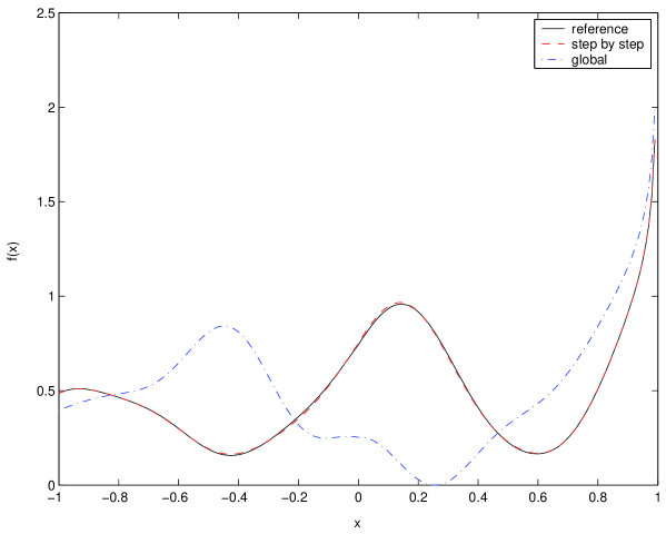
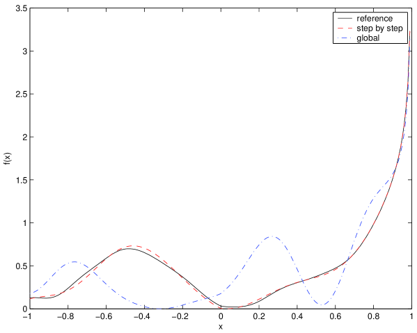
Figure 23: Comparison of the goodness of the two Nelder Mead minimization algorithms. The estimated density is always obtained for $q=5$. On the left panel, the reference density is calculated with $q=5$ and on the right one with $q=10$.

The figure 23 illustrates the convergence of this procedure in the case of a numerical experiment that unfolds as follows :

1. we generate a reference density with a chosen $q$,

2. we apply the two procedures using the Nelder-Mead method,

3. we compare the accuracy of the two estimated densities to the reference density,

4. step (1) and (2) are iterated one thousand times.

The two graphs show the efficiency of the step by step method. On the left panel, the reference density has been drawn for $q=5$ and we estimated the densities for $q=5$ too. The best estimated density is irrevocably the one obtained by the iterative procedure. On the right panel, we account for the fact that the density should have an infinite number of parameters (see equation (46)) or, at least, that the right order $q$ in (49) is generally unknown. that is why we have generated a reference density with $q=10$ and performed the estimation for $q=5$ only to investigate the effect of the truncation on the accuracy of the two approaches. The result obtained for a randomly chosen simulation is displayed on the right panel of figure 23. One more time, the iterative method gives better results than global approach.

[Insert figure 23 about here]

While we have not been able to prove the convergence of the “step by step” procedure, our numerical simulations show that it provides estimates that are always close to the true parameter values (within the uncertainty predicted by proposition 3). In addition, these estimates are almost always more accurate than the estimates obtained by use of the genetic algorithm, due to the very slow convergence of this algorithm.

Symbol	Company	Market	Sector	Cap.
BKS	Barnes & Noble Inc.	NYSE	dist. (c)	1.62
VLO	Valero Energy corp (new)	NYSE	energy	1.70
DHI	DR Horton inc.	NYSE	dist. (c)	1.83
LEN	Lennar corp CL a common	NYSE	dist. (c)	1.85
TCB	TCF Financial Corp.	NYSE	financial	1.92
NYB	New York Bancorp inc.	NYSE	financial	2.17
FNF	Fidelity Natl Financial inc.	NYSE	financial	2.27
MCHP	Microchip Technology inc.	Nasdaq	tech.	2.99
WPO	Washington post co clb	NYSE	com.	3.71
GILD	Gilead Science inc.	Nasdaq	dist. (nc)	3.90
GM	General Motors co.	NYSE	dist. (c)	31.81
PG	Procter & Gamble co.	NYSE	dist. (nc)	84.30
IBM	Intel Business Machines corp.	NYSE	tech.	108.01
CSCO	Cisco Systems inc.	Nasdaq	com.	112.26
MRK	Merck & co inc.	NYSE	dist. (nc)	112.73
KO	Coca-Cola co.	NYSE	dist. (nc)	118.97
AIG	American intl group inc.	NYSE	financial	125.58
INTC	Intel corp.	Nasdaq	tech.	140.77
WMT	Wall-Mart Stores inc.	NYSE	dist. (c)	144.61
C	Citigroup	NYSE	financial	148.79
PFE	Pfizer inc.	NYSE	dist. (nc)	198.20
XOM	Exxon mobile corporation	NYSE	energy	199.19
MSFT	Microsoft corp.	Nasdaq	tech.	239.81
GE	General Electrics co.	NYSE	industrial	290.44

Table 1: Average capitalization (in billion dollars) of every assets over the whole period (01/01/1994 to 12/31/2003) and their characteristics.

Asset	$d$	$d_{gph}$	$d_{hurst}$
BKS	0.19  (0.04)	0.36  (0.02)	0.44
VLO	0.23  (0.04)	0.32  (0.02)	0.44
DHI	0.34  (0.04)	0.34  (0.02)	0.50
LEN	0.31  (0.05)	0.34  (0.02)	0.53
TCB	0.31  (0.04)	0.35  (0.02)	0.43
NYB	0.00  (0.06)	0.33  (0.02)	0.37
FNF	0.25  (0.04)	0.34  (0.02)	0.28
MCHP	0.19  (0.04)	0.45  (0.02)	0.42
WPO	0.45  (0.04)	0.28  (0.02)	0.46
GILD	0.37  (0.06)	0.44  (0.02)	0.42
GM	-0.30  (0.04)	0.30  (0.02)	0.30
PG	0.22  (0.05)	0.41  (0.02)	0.53
IBM	0.21  (0.05)	0.36  (0.02)	0.44
CSCO	0.33  (0.06)	0.47  (0.02)	0.51
MRK	0.22  (0.05)	0.37  (0.02)	0.49
KO	0.16  (0.05)	0.41  (0.02)	0.55
AIG	0.10  (0.03)	0.44  (0.02)	0.48
INTC	0.23  (0.06)	0.38  (0.02)	0.53
WMT	0.31  (0.04)	0.42  (0.02)	0.46
C	-0.02  (0.04)	0.40  (0.02)	0.51
PFE	0.16  (0.05)	0.40  (0.02)	0.55
XOM	-0.09  (0.04)	0.41  (0.02)	0.49
MSFT	0.21  (0.03)	0.43  (0.02)	0.53
GE	0.04  (0.06)	0.44  (0.02)	0.50

Table 2: Estimation of the long memory parameter, $d$, by our method and different semi-parameter methods (Geweke and Porter-Hudak (GPH) and Hurst) for all the assets, over the whole period (from 01/01/1994 to 12/31/2003). For the GPH estimator we also give the standard deviation.

		Whole	Before	After
		period	bubble burst	bubble burst
CSCO	d ($\bar{\sigma}$)	0.33 (0.06)	0.27 (0.04)	0.18 (0.04)
	w	(0.12)	(0.57)	(0.55)
	$\alpha$	(0.12)	(0.80)	(0.55)
MRK	d ($\bar{\sigma}$)	0.22 (0.05)	0.30 (0.04)	0.08 (0.04)
	w	(0.43)	(0.43)	(0.45)
	$\alpha$	(0.31)	(0.66)	(0.39)
KO	d ($\bar{\sigma}$)	0.16 (0.05)	0.19 (0.04)	0.20 (0.05)
	w	(0.46)	(0.41)	(0.47)
	$\alpha$	(0.62)	(0.66)	(0.41)
AIG	d ($\bar{\sigma}$)	0.10 (0.03)	0.26 (0.05)	-0.32 (0.04)
	w	(0.64)	(0.61)	(0.12)
	$\alpha$	(0.64)	(0.45)	(0.85)
MSFT	d ($\bar{\sigma}$)	0.21 (0.03)	0.34 (0.04)	0.00 (2.$10^{5}$)
	w	(0.66)	(0.70)	(0.05)
	$\alpha$	(0.54)	(0.50)	(0.30)

Table 3: Estimation of the long memory parameter $d$ (and its satandard deviation), the parameter $\alpha$ and the weight $w$ by using the auto-correlations method for some large capitalizations, over the whole period (from 01/01/1994 to 12/31/2003).

References

- [1] \harvarditem[Abramowitz and Stegun]Abramowitz and Stegun1965abramowitz65 Abramowitz, M., and I. Stegun, 1965, Handbook of Mathematical Functions. (Dover).
- [2] \harvarditem[Andersen, Bollerslev, Diebold, and Ebens]Andersen, Bollerslev, Diebold, and Ebens2001aandersen01 Andersen, T. G., T. Bollerslev, F. X. Diebold, and H. Ebens, 2001a, The distribution of realised stock return volatility, Journal of Financial Economics 61, 43–76.
- [3] \harvarditem[Andersen, Bollerslev, Diebold, and Labys]Andersen, Bollerslev, Diebold, and Labys2001bandersen01b Andersen, T. G., T. Bollerslev, F. X. Diebold, and P. Labys, 2001b, The distribution of exchange rate volatility, Journal of the American Statistical Association 96, 42–55.
- [4] \harvarditem[Andersen, Bollerslev, Diebold, and Labys]Andersen, Bollerslev, Diebold, and Labys2003andersen02 Andersen, T. G., T. Bollerslev, F. X. Diebold, and P. Labys, 2003, Modeling and forecasting realized volatility, Econometrica 71, 529–626.
- [5] \harvarditem[Baillie, Bollerslev, and Mikkelsen]Baillie, Bollerslev, and Mikkelsen1996baillie96 Baillie, R. T., T. Bollerslev, and H. O. Mikkelsen, 1996, Fractionally integrated generalized autoregressive conditional heteroskedasticity, Journal of Econometrics 74, 3–30.
- [6] \harvarditem[Banerjee]Banerjee1992banerjee92 Banerjee, A.V., 1992, A simple model of herd behavior, Quaterly Journal of Economics 110 (3), 797–817.
- [7] \harvarditem[Banerjee]Banerjee1993banerjee93 Banerjee, A.V., 1993, The economics of rumours, Review of Economic Studies 60, 309–327.
- [8] \harvarditem[Barberis and Thaller]Barberis and Thaller2003BT2003 Barberis, N., and R. Thaller, 2003, A survey of behavioral finance, in G. M. Constantinides, M. Harris, and R. M. Stulz, eds.: Handbook of the Economics of Finance (Elsevier Science).
- [9] \harvarditem[Barndorff-Nielsen and Shephard]Barndorff-Nielsen and Shephard2002abarndorff01 Barndorff-Nielsen, O. E., and N. Shephard, 2002a, Estimating Quadratic Variation Using Realized Volatility, Journal of Applied Econometrics 17, 457–477.
- [10] \harvarditem[Barndorff-Nielsen and Shephard]Barndorff-Nielsen and Shephard2002bbarndorff02 Barndorff-Nielsen, O. E., and N. Shephard, 2002b, Econometric Analysis of Realised Volatility and its Use in Estimating Stochastic Volatility Models, Journal of the Royal Statistical Society, Series B 64, 253–280.
- [11] \harvarditem[Bingham, Goldie, and Teugels]Bingham, Goldie, and Teugels1989BGT89 Bingham, N. H., C. M. Goldie, and J. L. Teugels, 1989, Regular variations. (Cambridge University Press).
- [12] \harvarditem[Bollen and Inder]Bollen and Inder2002bollen02 Bollen, B., and B. Inder, 2002, Estimating daily volatility in financial markets utilizing intraday data, Journal of Empirical Finance 9, 551–562.
- [13] \harvarditem[Brockwell and Davis]Brockwell and Davis1990brockwell90 Brockwell, P. J., and R. A. Davis, 1990, Times Series : Theory and Methods. (Springer-Verlag, second edition).
- [14] \harvarditem[Chou]Chou1988chou88 Chou, R. Y., 1988, Volatility persistence and stock valuations: some empirical evidence using GARCH, Journal of Applied Econometrics 3, 279–294.
- [15] \harvarditem[Clark]Clark1973clark73 Clark, P. K., 1973, A subordinated stochastic process model with finite variance for speculative prices, Econometrica 41, 135–155.
- [16] \harvarditem[Cont and Bouchaud]Cont and Bouchaud2000cont00 Cont, R., and J.P. Bouchaud, 2000, Herd behaviour and aggregate fluctuations in financial markets, Macroeconomic Dynamics 4, 170–195.
- [17] \harvarditem[Dacoragna, Müller, Nagler, Olsen, and Pictet]Dacoragna, Müller, Nagler, Olsen, and Pictet1993Dacorogna93 Dacoragna, M.M., U.A Müller, R.J. Nagler, R.B. Olsen, and O.V. Pictet, 1993, A geographical model for the daily and weekly seasonal volatility in the foreign exchane market, Journal of International Money and Finance 112, 413–438.
- [18] \harvarditem[Davidson and Sibbersten]Davidson and Sibbersten2005davidson05 Davidson, J., and P. Sibbersten, 2005, Generating schemes for long memory processes : regimes, aggregation and linearity, Journal of Econometrics.
- [19] \harvarditem[Di Matteo, Aste, and Dacorogna]Di Matteo, Aste, and Dacorogna2005Dacorogna05 Di Matteo, T., T. Aste, and M. M. Dacorogna, 2005, Long-term memories of developed and emerging markets: Using the scaling analysis to characterize their stage of development, Journal of Banking and Finance 29, 827–851.
- [20] \harvarditem[Diebold and Inoue]Diebold and Inoue2001diebold01 Diebold, F. X., and A. Inoue, 2001, Long memory and regime switching, Journal of Econometrics 105, 131–159.
- [21] \harvarditem[Ding, Granger, and Engle]Ding, Granger, and Engle1993ding83 Ding, Z., C. W. J. Granger, and R. F. Engle, 1993, A long memory property of stock market returns and a new model, Journal of Empirical Finance 1, 83–106.
- [22] \harvarditem[Dorsey and Mayer]Dorsey and Mayer1995dorsey95 Dorsey, R. E., and W. J. Mayer, 1995, Genetic Algorithms for Estimation Problems with Multiple Optima, Non-Differentiability, and other Irregular Features, Journal of Business and Economic Statistics 13, 53–66.
- [23] \harvarditem[Fama]Fama1965fama65 Fama, E. F., 1965, The behavior of stock-market prices, Journal of Business 38, 34–105.
- [24] \harvarditem[Froot, Scharfstein, and Stein]Froot, Scharfstein, and Stein1992froot92 Froot, K.A., D.S. Scharfstein, and J.C. Stein, 1992, Herd on the street: Informational inefficiencies in a market with short-term speculation, Journal of Finance 47 (4), 1461–1484.
- [25] \harvarditem[Gadea, Sabaté, and Serrano]Gadea, Sabaté, and Serrano2004gadea04 Gadea, M. D., M. Sabaté, and J. M. Serrano, 2004, Structural breaks and thier trace in the memory inflation rate series in the long-run, Journal of International Financial Markets, Institutions & Money 14, 117–134.
- [26] \harvarditem[Geweke and Porter-Hudak]Geweke and Porter-Hudak1983geweke83 Geweke, J., and S. Porter-Hudak, 1983, The estimation and application of long-memory time series model, Journal of Time Series Analysis 4, 221–238.
- [27] \harvarditem[Golberg]Golberg1989goldberg89 Golberg, D. E., 1989, Genetic Algorithm in Search, Optimization and Learning. (Addison-Wesley).
- [28] \harvarditem[Gonçalves and Gouriéroux]Gonçalves and Gouriéroux1988goncalves88 Gonçalves, E., and C. Gouriéroux, 1988, Agrégation de processus autorégressifs d’ordre 1, Annales d’Economies et de Statistique 12, 127–149.
- [29] \harvarditem[Gouriéroux and Jasiak]Gouriéroux and Jasiak2001gourieroux01 Gouriéroux, C., and J. Jasiak, 2001, Memory and infrequent breaks, Economics Letters 70, 29–41.
- [30] \harvarditem[Granger and Hyung]Granger and Hyung2004granger04 Granger, C. W. J., and N. Hyung, 2004, Occasional structural breaks and long memory with an application to the S&P 500 absolute stock returns, Journal of Empirical Finance 11, 399–421.
- [31] \harvarditem[Granger and Joyeux]Granger and Joyeux1980granger80 Granger, C. W. J., and R. Joyeux, 1980, An introduction to long-memory time series models and fractional differencing, Journal of Time Series Analysis 1, 15–30.
- [32] \harvarditem[Hosking]Hosking1996hosking96 Hosking, J. R. M., 1996, Asymptotic distribution of the sample mean, autocovariances, and autocorrelations of long-memory time series, Journal of Econometrics 73, 261–284.
- [33] \harvarditem[Hurst]Hurst1951hurst51 Hurst, H., 1951, Long Term Storage Capacity of Reservoirs, Transaction of the American Society of Civil Engineers 116, 770–799.
- [34] \harvarditem[Kearney and Daly]Kearney and Daly1998kearney98 Kearney, C., and K. Daly, 1998, The causes of stock market volatility in Australia, Applied Financial Economics 8, 597–605.
- [35] \harvarditem[Kirman]Kirman1993kirman93 Kirman, A., 1993, Ants, rationality and recruitment, Quaterly Journal of Economics 108, 135–156.
- [36] \harvarditem[Lagarias, Reeds, Wright, and Wright]Lagarias, Reeds, Wright, and Wright1998lagarias98 Lagarias, J. C., J. A. Reeds, M. H. Wright, and P. E. Wright, 1998, Convergence Properties of the Nelder-Mead Simplex Method in Low Dimensions, SIAM Journal of Optimization 9(1), 112–147.
- [37] \harvarditem[Lo]Lo1991lo91 Lo, A. W., 1991, Long term memory in stock market prices, Econometrica 59, 1779–313.
- [38] \harvarditem[Mandelbrot]Mandelbrot1963mandelbrot63 Mandelbrot, B., 1963, The variation of certain speculative prices, Journal of Business 36, 394–419.
- [39] \harvarditem[Mandelbrot]Mandelbrot1972mandelbrot72 Mandelbrot, B., 1972, Statistical Methodology for Non-Periodic Cycles : From the covariance to R/S analysis, Annals of Economic and Social Measurement 1, 259–299.
- [40] \harvarditem[Mandelbrot]Mandelbrot1975mandelbrot75 Mandelbrot, B., 1975, Limit Theorems on the Self-Normalized Range for Weakly and Strongly Dependent Processes, Zeitschrift für Wahrscheinlichkeitstheorie und verwandte Gebiete 31, 271–285.
- [41] \harvarditem[Mandelbrot and Taqqu]Mandelbrot and Taqqu1979mandelbrot79 Mandelbrot, B., and M. Taqqu, 1979, Robust R/S Analysis of Long-Run Serial Correlation, Bulletin of the International Statistical Institute 48 (2), 59–104.
- [42] \harvarditem[Nelder and Mead]Nelder and Mead1965Nelder1965 Nelder, J. A., and R. Mead, 1965, A Simplex Method for Function Minimization, Computer Journal 7, 308–313.
- [43] \harvarditem[Newey and McFadden]Newey and McFadden1994newey94 Newey, W. K., and D. L. McFadden, 1994, Large sample estimation and hypothesis testing, in R. F. Engle, and D. L. McFadden, eds.: Handbook of Econometrics (Elsevier Science, ).
- [44] \harvarditem[Orlean]Orlean1995orlean95 Orlean, A., 1995, Bayesian interactions and collective dynamics of opinion: Herd behaviour and mimetic contagion, Journal of Economic Behavior anc Organization 28, 257–274.
- [45] \harvarditem[Pagan and Ullah]Pagan and Ullah1999pagan99 Pagan, A., and A. Ullah, 1999, Nonparametric Econometrics. (Cambridge University Press).
- [46] \harvarditem[Price and Storn]Price and Storn1997price97 Price, K., and R. Storn, 1997, Differential Evolution, Dr. Doob’s Journal April, 18–24.
- [47] \harvarditem[Roll]Roll1984roll84 Roll, R., 1984, A Simple Implicit Measure of the Effective Bid-Ask Spread in an Efficient Market, The Journal of Finance 39, 1027–1039.
- [48] \harvarditem[Sadorsky]Sadorsky2003sadorsky03 Sadorsky, P., 2003, The macroeconomic determinants of technology stock price volatility, Review of Financial Economics 12, 191–205.
- [49] \harvarditem[Schwert]Schwert1989schwert89 Schwert, G.W., 1989, Why does stock market volatility chane over time ?, Journal of Finance 44, 1115–1153.
- [50] \harvarditem[Shiller]Shiller1989shiller89 Shiller, R.J., 1989, Market Volatility. (MIT Press).
- [51] \harvarditem[Shiller]Shiller2000shiller00 Shiller, R.J., 2000, Irrational Exuberance. (Princeton University Press).
- [52] \harvarditem[Sornette]Sornette2003sornette03 Sornette, D., 2003, Why Stock Markets Crash. (Princeton University Press Princeton, NJ).
- [53] \harvarditem[Taylor]Taylor1986Taylor86 Taylor, S. J., 1986, Modelling Financial Time Series. (John Wiley Chichester).
- [54] \harvarditem[Teverovsky, Taqqu, and Willinger]Teverovsky, Taqqu, and Willinger1999teverovsky99 Teverovsky, V., M. S. Taqqu, and W. Willinger, 1999, A critical look at Lo’s modified R/S statistic, Journal of Statistical Planning and Inference 80, 211–227.
- [55] \harvarditem[van der Vaart]van der Vaart2000vaart00 van der Vaart, A. W., 2000, Asymptotic Statistics. (Cambridge University Press).
- [56]