Heteroclinic connections in plane Couette flow

Abstract

Plane Couette flow transitions to turbulence for $Re\approx 325$ even though the laminar solution with a linear profile is linearly stable for all $Re$ (Reynolds number). One starting point for understanding this subcritical transition is the existence of invariant sets in the state space of the Navier Stokes equation, such as upper and lower branch equilibria and periodic and relative periodic solutions, that are quite distinct from the laminar solution. This article reports several heteroclinic connections between such objects and briefly describes a numerical method for locating heteroclinic connections. Computing such connections is essential for understanding the global dynamics of spatially localized structures that occur in transitional plane Couette flow. We show that the nature of streaks and streamwise rolls can change significantly along a heteroclinic connection.

1 Introduction

In plane Couette flow, the fluid between two parallel walls of fixed separation is driven by the motion of the walls in opposite directions. Even though the laminar solution is linearly stable for all $Re$ (Reynolds number) as shown by Kreiss et al. (1994), turbulent spots evolve into large turbulent patches for $Re$ exceeding the modest value of about $325$ (Bottin et al., 1998). These turbulent patches are sustained by the flow for very long, and possibly infinite, time intervals. From a dynamical point of view, the evolution of the velocity field corresponds to a trajectory in state space, and indefinitely sustained motion should correspond to invariant sets. Invariant sets in state space have the property that a trajectory that starts exactly on such a set stays on that set forever, and a trajectory that starts outside that set cannot land on it within a finite time interval although it can approach the invariant set rapidly. Thus a reasonable starting point for understanding when and why turbulence becomes sustained in plane Couette flow and other shear flows is not the loss of linear stability of laminar flow, which never happens in plane Couette flow, but the existence of invariant sets. Equilibria, traveling waves, periodic solutions, and relative periodic solutions are all invariant sets. The union of such sets can form chaotic saddles or chaotic attractors, invariant sets which may explain a good deal of the dynamics of shear flows (Schmiegel & Eckhardt, 1997). Thus the numerical computation of equilibria, traveling waves, periodic solutions, and relative periodic solutions (Nagata, 1990, 1997; Waleffe, 2003; Viswanath, 2007; Gibson et al., 2008b; Halcrow et al., 2008; Gibson et al., 2008a) is a step towards understanding the dynamics of plane Couette flow in the transitional regime.

We use a computational box of extent $0\leq x\leq 2\pi/\alpha$, $-1\leq y\leq 1$, and $0\leq z\leq 2\pi/\gamma$, with $\alpha=1.14$ and $\gamma=2.5$ (Waleffe, 2003), where $x$, $y$, $z$ are the streamwise, wall-normal, and spanwise coordinates, respectively. Likewise, $u$, $v$, $w$ are the three components of the velocity field. The boundary condition is periodic along $x$ and $z$, and no-slip at the walls. For comparison, the experimental setup of Bottin et al. (1998) is about a meter long with a separation between the walls of only $7$ mm. At the moment, small computational boxes are needed to keep the cost of computing invariant sets manageable. Nevertheless, small computational boxes are capable of picking up significant aspects of turbulent boundary layers and transitional dynamics, perhaps because some of the features of those regimes are localized in space. For instance, periodic and relative periodic orbits computed in a small box reproduce the formation and break-up of streaks in the near-wall region (Viswanath, 2007). Indeed, such solutions show that the spanwise advection of coherent structures could be a significant source of the spanwise variation of the root mean square value of the streamwise velocity. In addition, turbulent spots, which appear to play a key role in transition, are localized in space, although certain aspects of their dynamics depend upon the interaction with the external flow (Schumacher & Eckhardt, 2001).

In this article, we report three heteroclinic connections between equilibrium (or steady) solutions of plane Couette flow at $Re=400$, where the $Re$ is based on half the difference in velocity between the moving walls, half the distance between the walls, and the kinematic viscosity of the fluid. Basic data for six such solutions, with the first one being the laminar solution, is given by Table 1 (for detailed data sets the reader can consult Channelflow.org and Halcrow (2008)). The equations of plane Couette flow are unchanged by the shift-reflect and shift-rotate transformations defined in Section 3. All the equilibria lie in the $S$-invariant subspace, which is the space of velocity fields invariant under both transformations. The equilibria ${\text{EQ}_{1}}$ and ${\text{EQ}_{2}}$ are called lower and upper branch solutions (Nagata, 1990; Waleffe, 2003). The heteroclinic connections reported here are from ${\text{EQ}_{3}}$, ${\text{EQ}_{4}}$, and ${\text{EQ}_{5}}$ to ${\text{EQ}_{1}}$; and from ${\text{EQ}_{1}}$ to ${\text{EQ}_{2}}$.

	$I=D$	$E$	$E_{roll}/E$	$d(W^{u})$	$d(W^{u}_{S})$	$\lambda_{0}$	$Re_{\tau}$
${\text{EQ}_{0}}$	1	1	0	0	0	-0.00616850	$40$
${\text{EQ}_{1}}$	1.429258	0.817778	0.000330	1	1	0.05012078	$47.82$
${\text{EQ}_{2}}$	3.043675	0.468225	0.018323	8	2	0.05558362	$69.78$
${\text{EQ}_{3}}$	1.317683	0.829378	0.000759	4	2	$0.03397837\pm 0.01796294\,\imath$	$45.92$
${\text{EQ}_{4}}$	1.453682	0.746056	0.002515	6	3	0.03064964	$48.23$
${\text{EQ}_{5}}$	2.020135	0.644223	0.003511	11	4	$0.07212161\pm 0.04074989\,\imath$	$56.85$

Table 1: Basic statistics for equilibria at $Re=400$. ${\text{EQ}_{0}}$ is the laminar solution of plane Couette flow. The rate of energy input $I$ and the rate of dissipation $D$ are both normalized to be $1$ for the laminar state. So is the total kinetic energy denoted by $E$. $E_{roll}/E$ is the fraction of the total kinetic energy in the rolls. The dimension of the unstable manifold is $d(W^{u})$, while $d(W^{u}_{S})$ is the dimension of the intersection of the unstable manifold with the $S$-invariant subspace. $\lambda_{0}$ is the eigenvalue with the greatest real part, and $Re_{\tau}$ is the width of the channel in wall units.

In the presence of continuous rotation symmetry and discrete reflection symmetry, the existence of heteroclinic cycles follows from the normal form of certain codimension-2 bifurcations (Kuznetsov, 1998). Abshagen et al. (2004, 2005) have shown that Taylor-Couette flow with a stationary outer cylinder undergoes a codimension-2 bifurcation, the normal form of which implies the existence of a heteroclinic cycle. That the basic laminar solution of this Taylor-Couette flow undergoes a sequence of supercritical bifurcations, making it possible to track bifurcations while computing only linearly stable solutions, while the transition in plane Couette flow is subcritical is just one difference from our work. Notably, the computations of Abshagen et al. (2004) use a domain and boundary conditions that match their experimental setup. We do not compute codimension-2 bifurcations, although we return to that point and the influential thesis of Schmiegel (1999) in Section 4. In addition, our computations of heteroclinic connections are explicit and make use of the eigenvalues and eigenvectors of the linearizations around the equilibria.

Instead, our computations rely on the simple principle that an object of dimension $k$ is likely to intersect in a stable way an object whose codimension in state space is less than or equal to $k$. At the bottom, this is nothing more than the fact that two submanifolds in general position can intersect if the sum of their dimensions is greater than or equal to the dimension of the state space(whether they actually intersect is a subtle question that is central to the “structural stability” of ergodic dynamical systems (Smale, 1967)). For an illustration in the nonlinear setting, see Abraham & Shaw (1992). Kevrekidis et al. (1990) (see Section 5 of their paper) make elegant use of this principle and of invariant subspaces implied by discrete symmetries of the underlying PDE to numerically deduce the existence of a heteroclinic connection in the Kuramoto-Sivashinsky equation. Indeed, they comment that their work may have implications for shear flows. With regard to the heteroclinic connections presented here, it is significant to note from Table 1 that the codimension of the stable manifold in the $S$-invariant space (which is equal to $d(W^{u}_{S})$) of ${\text{EQ}_{1}}$ is less than the value of $d(W^{u}_{S})$ for $\text{EQ}_{i}$ with $i=3,4,5$. Thus it is not surprising that the unstable manifolds of $\text{EQ}_{i}$ with $i=3,4,5$ intersect the stable manifold of ${\text{EQ}_{2}}$ in a stable way (i.e., robustly with respect to small changes of system parameters).

All the equilibria in Table 1, except ${\text{EQ}_{5}}$, have well-formed streaks, which means that the streamwise velocity has pronounced variation in the spanwise direction. The streaks are accompanied by streamwise rolls which is the typical situation for boundary layers (Kim et al., 1971). Streaks and streamwise rolls are also found near the edges of turbulent spots (Dauchot & Daviaud, 1995; Tillmark, 1995; Schumacher & Eckhardt, 2001). They could be relevant to the wavelike manner in which the turbulent spots spread to form patches. In this regard, we note that heteroclinic connections are important to obtaining a global picture of the dynamics in state space. They can be useful for the physical space picture as well, as shown by the dramatic change in the balance between rolls and streaks along the heteroclinic connection from ${\text{EQ}_{5}}$ to ${\text{EQ}_{1}}$. In Section 3, we present a state space plot in the manner of Gibson et al. (2008b) to show how the heteroclinic connections at $Re=400$ are related to one another.

2 Finding and verifying heteroclinic connections

The discretization of the computational box used $32$ Fourier points in the $x$ direction, $35$ Chebyshev points in the $y$ direction, and $32$ Fourier points in the $z$ direction. Direct numerical simulation of plane Couette flow was performed using Channelflow.org (Gibson, 2007). The equilibria listed in Table 1 were found using GMRES-hookstep iterations (Viswanath, 2007). If the velocity fields of the equilibria are integrated for a certain fixed time, they are nearly unchanged. Yet the evolution of perturbations under such an integration can be used along with the Arnoldi iteration to determine all unstable eigenvalues and eigenvectors, as well a set of the least contracting stable eigenvalues and eigenvectors (Viswanath, 2007). Such a computation was used to produce the information about the unstable manifolds of the equilibria listed in Table 1.

The shift-reflect and shift-rotate transformations of a velocity field are given by

$$s_{1}[u,v,w](x,y,z) =[u,v,-w](x+L_{x}/2,y,-z),$$

$$s_{2}[u,v,w](x,y,z) =[-u,-v,w](-x+L_{x}/2,-y,z+L_{z}/2),$$ (1)

respectively, where $L_{x}$ and $L_{z}$ are the periods of the computational box in the $x$ and $z$ directions. If either transformation is applied to a trajectory of plane Couette flow, one gets another trajectory of plane Couette flow. The space of velocity fields unchanged by both $s_{1}$ and $s_{2}$ is an invariant subspace called the $S$-invariant space in Gibson et al. (2008b). All the computations in this paper are restricted to this invariant space. The norm used over velocity fields of plane Couette flow throughout this paper is the square root of the kinetic energy, with a normalization that makes the norm of the laminar solution equal to $1$.

In a heteroclinic connection, the velocity field of plane Couette flow varies over a time (or $t$) interval infinite in both senses, approaching equilibria as $t\rightarrow-\infty$ and as $t\rightarrow\infty$. Those are the initial and final equilibria of the heteroclinic connection. Since it is impossible to integrate over an infinite time interval, our computed heteroclinic connections start out in the linearized neighborhood and close to the initial or “out” equilibrium ${\bf u}_{\text{\tiny out}}$, and end in the linearized neighborhood close to the final or “in” equilibrium ${\bf u}_{\text{\tiny in}}$, after a finite interval of time. For the heteroclinic connections that go from ${\text{EQ}_{3}}$ and ${\text{EQ}_{5}}$ to ${\text{EQ}_{1}}$, the initial point on the computed heteroclinic connection is a perturbation using the two dimensional eigenspace that corresponds to the complex pair of eigenvalues with the greatest real part. It is reasonable to look in that space because all except a proper subspace of trajectories that originate near an equilibrium point are tangent to the leading eigenspace, which is $1$-dimensional if the eigenvalue with the largest real part is real and simple and $2$-dimensional if a simple complex pair. For the same reason, it is perhaps surprising that the heteroclinic connection from ${\text{EQ}_{4}}$ to ${\text{EQ}_{1}}$ is found using an eigenspace corresponding to a complex pair with real part less than that of one other eigenvalue.

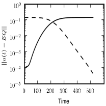
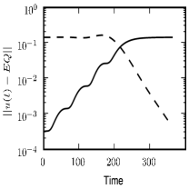
(a) (b) (c)

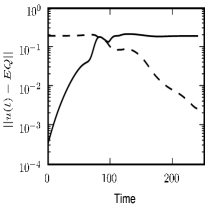
Figure 1: Plots of distances from the initial (solid line) and final (dashed line) equilibria to the velocity field at varying times along the computed heteroclinic connection. (a), (b), (c) correspond to the heteroclinic connections into ${\text{EQ}_{1}}$ from ${\text{EQ}_{3}}$, ${\text{EQ}_{4}}$, and ${\text{EQ}_{5}}$, respectively.

Let ${\bf e}^{(1)}$, ${\bf e}^{(2)}$ be an orthonormal basis for the two-dimensional eigenspace that corresponds to a complex eigenvalue pair of the equilibrium ${\bf u}_{\text{\tiny out}}$. The span will be tangent to the unstable manifold at the equilibrium. We consider the set of velocity fields of plane Couette flow that at the initial time $T=0$ lie on a circle of radius $r$:

$${\bf u}(0)_{\phi}={\bf u}_{\text{\tiny out}}+r({\bf e}^{(1)}\cos\phi+{\bf e}^{(2)}\sin\phi)\,.$$

For a small and fixed value of $r$, we search for a point on this circle which evolves to make the closest approach to another equilibrium, ${\bf u}_{\text{\tiny in}}$. Let

$$G(\phi)=\min_{T}\lVert{\bf u}(T)_{\phi}-{\bf u}_{\text{\tiny in}}\rVert,$$

where ${\bf u}(T)_{\phi}$ is the velocity field that results from evolving the velocity field ${\bf u}(0)_{\phi}$ for time $T$ and where the minimizing value of $T$ is the time of the first local minimum greater than a certain threshold. The closest approach is the minimum of $G(\phi)$ over $0\leq\phi<2\pi$. Since $G(\phi)$ is a function of a single real variable, it can be minimized using any one of a number of well-known and effective methods. The computation of heteroclinic connections sketched above uses a first order asymptotic boundary condition at the initial equilibrium. For small systems, it is possible to use an asymptotic boundary condition at the final equilibrium as well. For an example, see Demmel et al. (2000).

For the computed heteroclinic connections from ${\text{EQ}_{3}}$, ${\text{EQ}_{4}}$, and ${\text{EQ}_{5}}$ to ${\text{EQ}_{2}}$, the chosen values of $r$ were 0.0001, 0.0003, and 0.0004, respectively. Figure 1 shows data for the three computed heteroclinic connections. In each plot of that figure, the solid line is tiny at the beginning but rises exponentially while the dashed line is flat. Therefore, we conclude that the initial part of each computed heteroclinic connection is in a region where its time evolution is governed by the linearization around its initial equilibrium. Similarly, we can conclude that the final part is in a region where the evolution is governed by the linearization around the final equilibrium.

To verify the computed heteroclinic connections using another code, it could be necessary to use three stages. The computed connection from ${\text{EQ}_{5}}$ to ${\text{EQ}_{1}}$, for instance, spends about $75$ time units near the initial equilibrium and more than $100$ units near the final equilibrium, as evident from Figure 1. Using the data in Table 1, one may easily estimate that the loss of precision in those two stages is more than $3$ digits. As the equilibria themselves are computed with only about $4$ or $5$ digits of precision, one has to do the verification in segments. Such a verification of Figure 1, which was performed using a completely independent code (Viswanath, 2007), and the applicability of shadowing theorems about numerical trajectories (Palmer, 2000) leave little doubt that the computed heteroclinic connections are real.

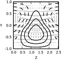
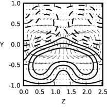
(a) (b) (c)

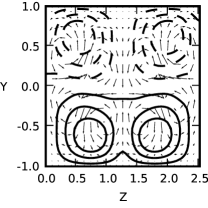
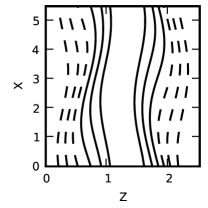
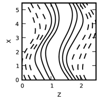
(d) (e) (f)

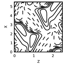
Figure 2: (a), (b), (c) correspond to ${\text{EQ}_{1}}$, ${\text{EQ}_{4}}$, ${\text{EQ}_{5}}$, while (d), (e), (f) correspond to ${\text{EQ}_{1}}$, ${\text{EQ}_{3}}$, ${\text{EQ}_{5}}$, respectively (there is very little difference in the plots for ${\text{EQ}_{3}}$ and ${\text{EQ}_{4}}$). The quiver plots in the top row show the streamwise averaged velocity components $v$ and $w$ in the $y-z$ plane. The six contour lines of the streamwise averaged $u$ component are equispaced in $(u_{max},-u_{max})$, with $u_{max}$ being $0.44$, $0.27$ and $0.45$ for ${\text{EQ}_{1}}$, ${\text{EQ}_{4}}$ and ${\text{EQ}_{5}}$, respectively, and with the negative lines being dashed. The bottom plots show six contour lines of $u$ in the section $y=0$. The contour lines are equispaced in $(u_{max},-u_{max})$, with $u_{max}$ being $0.33$, $0.22$ and $0.18$ for ${\text{EQ}_{1}}$, ${\text{EQ}_{3}}$ and ${\text{EQ}_{5}}$, respectively, and with the negative lines being dashed. lots would be better, maybe a stride of 2 in both $x$ and $y$.]

3 Heteroclinic connections at $Re=400$

The top plots of Figure 2 show the correlation between the rolls and the position of the streaks. The equilibria ${\text{EQ}_{1}}$, ${\text{EQ}_{3}}$ and ${\text{EQ}_{4}}$ each have a single counter-rotating pair of rolls. The rolls distort the mean flow, which increases with $y$, and thus explain the position of the streaks in Figures 2a and b (Kerswell, 2005). ${\text{EQ}_{5}}$ has four counter-rotating pairs. From Figure 2f, we see that the mid-plane flow is not at all streaky for ${\text{EQ}_{5}}$.

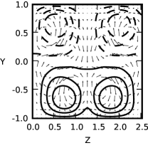
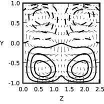
(a) (b) (c)

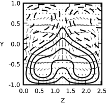
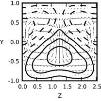
(d) (e)

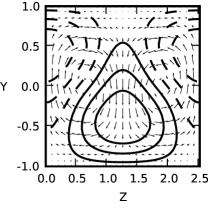
Figure 3: (a), (b), (c), (d), (e) are plots of the velocity field at $t=50$, $t=75$, $t=90$, $t=100$, and $t=150$, respectively, of the computed heteroclinic connection from ${\text{EQ}_{5}}$ to ${\text{EQ}_{1}}$ of Figure 1. The plots are similar to the ones in the top row of Figure 2, with values of $u_{max}$ being $0.48$, $0.44$, $0.36$, $0.46$ and $0.53$, respectively.

Figure 3 illustrates the manner in which the rolls change in form along the heteroclinic connection from ${\text{EQ}_{5}}$ to ${\text{EQ}_{1}}$. From Figure 1c, it is evident that for $t\in[75,125]$ the computed heteroclinic connection does not follow the linearized dynamics around its initial or final equilibrium. Figure 3 confirms that the rolls change in form within that interval. While the coexistence of rolls and streaks in turbulent boundary layers is well known (Kim et al., 1971), the sort of coalescence of rolls that is observed in Figure 3 is a new type of behavior.

The significance of the heteroclinic connections is that they give a global picture of the dynamics, a picture that cannot can be inferred from equilibria alone. To visualize global dynamics, it is essential to depict the equilibria and the heteroclinic connections between them in state space. The state space of plane Couette flow is infinite dimensional, and in the spatial discretization used for computing the heteroclinic connections, it is more than $6\times 10^{4}$, which is still much too large. Figure 4 uses a 3-dimensional projection of points in that state space, which was introduced by Gibson et al. (2008b), to depict the equilibria and the known connections between them.

Before explaining the projections used in Figure 4, we discuss why that figure can be considered a good visualization of the known heteroclinic connections of plane Couette flow at $Re=400$. It is typical to use projections to construct low dimensional models and these models are considered reasonable if they capture $90\%$ of the energy in the underlying flow, for instance. Such models use many more dimensions than just three axes, which is all that can be used in a depiction such as Figure 4. In addition, if the projected velocity field has $90\%$ of the energy, its normwise relative error can be as high as $30\%$. For these reasons, we do not use the amount of energy retained by the projection to judge the quality of depictions such as Figure 4.

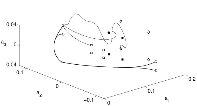
Figure 4: In the state space plot of the three heteroclinic connections at $Re=400$ above, ${\text{EQ}_{3}}$, ${\text{EQ}_{4}}$, and ${\text{EQ}_{5}}$, along with their images under the half shifts $\tau_{x}$, $\tau_{z}$ and $\tau_{xz}$, are denoted by the symbols $\square$,$\blacksquare$, and $\lozenge$ respectively. The laminar solution ${\text{EQ}_{0}}$ ($\odot$) is at the origin. ${\text{EQ}_{2}}$ and its images under the half shifts are denoted by $\circ$. The meaning of the axes is explained in the text.

Instead, we adopt a more geometric point of view. If a curve in a Hilbert space is projected onto a finite dimensional plane, it develops artificial cusps or corners at points where the tangent to the curve is orthogonal to the plane of projection. For instance, the projection of a smooth curve in $R^{3}$ to the normal plane at a fixed point on the curve has an artificial cusp (Widder, 1961, chapter 3). In Figure 4, we see that the heteroclinic connections can be wavy but do not have cusps. It is significant that the same projection gives a good depiction of all the three heteroclinic connections into ${\text{EQ}_{1}}$ and the heteroclinic connection from ${\text{EQ}_{1}}$ to the laminar solution, which is shown as a thick line.

To explain the coordinates $a_{1},a_{2},a_{3}$ in Figure 4, we define $\tau_{x}$ and $\tau_{z}$ as follows:

$$\tau_{x}[u,v,w](x,y,z)=[u,v,w](x+L_{x}/2,y,z),$$

$$\tau_{z}[u,v,w](x,y,z)=[u,v,w](x,y,z+L_{z}/2),$$

where $L_{x}$ and $L_{z}$ are the periods of the computational box along $x$ and $z$. In addition, $\tau_{xz}=\tau_{x}\tau_{z}$. For each equilibrium that is in the $S$-invariant subspace (1), one may apply $\tau_{x}$, $\tau_{z}$, and $\tau_{xz}$ to get three other equilibria that lie in the $S$-invariant subspace. In the same manner, one may use each computed heteroclinic connection to get three others. Only a single copy of each is shown in Figure 4.

Let $\hat{\bf u}_{2}$ be the velocity field of the upper-branch solution ${\text{EQ}_{2}}$, with the laminar velocity field subtracted. If ${\bf e}^{(i)}$ are defined by

$${\bf e}^{(1)} =c_{1}(1+\tau_{x}+\tau_{z}+\tau_{xz})\hat{\bf u}_{2}$$

$${\bf e}^{(2)} =c_{2}(1+\tau_{x}-\tau_{z}-\tau_{xz})\hat{\bf u}_{2}$$

$${\bf e}^{(3)} =c_{3}(1-\tau_{x}+\tau_{z}-\tau_{xz})\hat{\bf u}_{2}$$

$${\bf e}^{(4)} =c_{4}(1-\tau_{x}-\tau_{z}+\tau_{xz})\hat{\bf u}_{2},$$

with $c_{i}$ being normalizing constants, the ${\bf e}^{(i)}$ form an orthonormal set (Gibson et al., 2008b). For a given velocity field of plane Couette flow, the $a_{i}$ are obtained by subtracting the laminar flow from the velocity field and then taking the inner product with ${\bf e}^{(i)}$, where $i=1,2,3,4$.

The use of the upper branch equilibrium ${\text{EQ}_{2}}$ to define ${\bf e}^{(i)}$ and $a_{i}$ may appear arbitrary and to an extent it is. Heuristically it is a good choice because the computations of Gibson et al. (2008b) show that the dynamics of plane Couette flow, including turbulent episodes and trajectories that relaminarize quickly, appear to be trapped between the unstable manifolds of ${\text{EQ}_{2}}$ and its three images obtained by applying $\tau_{x}$, $\tau_{z}$ and $\tau_{xz}$ and the laminar solution.

EQ	$I=D$	$E$	$E_{roll}/E$	$d(W^{u})$	$d(W^{u}_{S})$	$\lambda_{0}$
${\text{EQ}_{0}}$	1	1	0	0	0	-0.010966
${\text{EQ}_{1}}$	1.710086	0.722516	0.002526	3	1	0.02524949
${\text{EQ}_{2}}$	2.076045	0.634025	0.006357	4	2	0.0441718

Table 2: The columns have the same meaning as in Table 1, but with the equilibria computed at $Re=225$.

4 A heteroclinic connection at $Re=225$

Table 2 gives data for ${\text{EQ}_{0}}$, ${\text{EQ}_{1}}$ and ${\text{EQ}_{2}}$ at $Re=225$. By comparing the dimensions of the unstable manifolds and their restrictions to the $S$-invariant space, we can infer that both ${\text{EQ}_{1}}$ and ${\text{EQ}_{2}}$ undergo bifurcations as $Re$ is increased from $225$ to $400$. The dimension of ${\text{EQ}_{1}}$’s unstable manifold is just $1$. By following that unstable manifold, we found a heteroclinic connection to ${\text{EQ}_{2}}$.

While the dimension of ${\text{EQ}_{1}}$’s unstable manifold in the $S$-invariant subspace is $1$, the codimension of ${\text{EQ}_{2}}$’s stable manifold in the same subspace is $2$. Based on that consideration alone a heteroclinic connection seems implausible. However, this heteroclinic connection is very likely related to a codimension-2 bifurcation. In such a scenario, the dimensions of the unstable manifold of the initial equilibrium and of the stable manifold of the final equilibrium must be compared only within the center manifold.

Schmiegel (1999) has systematically studied bifurcations of the solutions of plane Couette flow found by Nagata (1990) and Clever & Busse (1997) using a representation with about $1200$ modes. He has found heteroclinic connections where the saddle node bifurcation that gives rise to ${\text{EQ}_{1}}$ and ${\text{EQ}_{2}}$ is followed soon after by a pitchfork bifurcation as $Re$ is increased. The heteroclinic connection reported above is probably of that type.

To understand this heteroclinic connection better, it could be useful to think of $L_{z}$, the spanwise size of the computational box, as a parameter. In the parameter space with $Re$ and $L_{z}$ as the axes, the saddle-node bifurcations that give rise to ${\text{EQ}_{1}}$ and ${\text{EQ}_{2}}$ will form a curve. There will be another curve that corresponds to the pitchfork or the Hopf bifurcation. At the intersection of those curves, we will have a codimension-2 bifurcation. An advantage of realizing a heteroclinic connection using the normal form of a codimension-2 bifurcation is that we will get a heteroclinic cycle, not just a heteroclinic connection.

5 Conclusion

The unstable but recurrent coherent structures observed in turbulent boundary layers and in transitional flows are an aspect of turbulent flows. Invariant sets capture some features of these coherent structures and their dynamics. While the notion of coherent structures varies with the means used to identify them, the notion of invariant sets is much more precise. Compact but linearly unstable invariant sets in state space (such as equilibria, traveling waves, periodic orbits, partially hyperbolic tori) are exact solutions of the Navier-Stokes equation which correspond to sustained motions of the fluid.

As a turbulent flow evolves, every so often we catch a glimpse of a familiar pattern. In some instances, turbulent dynamics visualized in state space appears pieced together from close visitations of equilibria connected by transient interludes. These turbulent interludes themselves reflect close passes to other invariant sets in state space, such as unstable periodic orbits. Such an approach to turbulence based on a repertoire of recurrent spatio-temporal patterns, which would be periodic or relative periodic orbits in state space, was proposed by Christiansen et al. (1997) as an implementation of Hopf (1948)’s view that turbulent flows are ergodic trajectories in state space. A similar approach has been suggested by Narasimha (1989), who refers to these patterns as molecules of turbulence.

The heteroclinic orbits that we present here could be the initial steps in charting an atlas of the dynamics of plane Couette flow; close passages to equilibria could be identified with nodes of Markov graph to give a coarse form of symbolic dynamics, and then these heteroclinic cycles would be directed links connecting nodes of the Markov graph. The lower branch equilibrium ${\text{EQ}_{1}}$, along with the equilibria which connect back to it, appear to form a part of the state space boundary dividing two regions: one laminar the other turbulent. Turbulent trajectories appear to be trapped between that boundary and the unstable manifolds of the upper branch equilibrium ${\text{EQ}_{2}}$, as illustrated by Gibson et al. (2008b).

The emergence and disappearance of these heteroclinic connections can also be diagnostic. The disappearance of the ${\text{EQ}_{1}}$ to ${\text{EQ}_{2}}$ connection is reminiscent of other global bifurcations occurring in simpler dynamical systems. For instance, in the Lorenz system a series of such bifurcations occur as the “Rayleigh” number is increased (Jackson, 1989). For plane Couette flow, such bifurcations could be useful for marking the onset of turbulence.

Future work in this direction should serve to clarify such points. It is still not entirely clear what happens at the global bifurcations involved in the creation and annihilation of these heteroclinic connections. Furthermore, lists of equilibria and of the heteroclinic connections between them found so far should by no means be considered exhaustive. Further investigation of plane Couette flow as well as other geometries will most likely turn up other dynamically important invariant sets, and more heteroclinic connections between them.

Acknowledgments. The authors thank Y. Duguet and L. van Veen for helpful discussions. D.V. was partly supported by NSF grants DMS-0407110 and DMS-0715510. He thanks the mathematics department of the Indian Institute of Science, Bangalore, for its hospitality and support. P.C., J.F.G. and J.H. thank G. Robinson, Jr. for support. J.H. thanks R. Mainieri and T. Brown, Institute for Physical Sciences, for partial support. Special thanks to the Georgia Tech Student Union which generously funded our access to the Georgia Tech Public Access Cluster Environment (GT-PACE).

References

- Abraham & Shaw (1992) Abraham, R. & Shaw, C. 1992 Dynamics, the Geometry of Behavior. Addison-Wesley.
- Abshagen et al. (2004) Abshagen, J., Lopez, J. M., Marques, F. & Pfister, G. 2004 Mode competition of rotating waves in reflection-symmetric Taylor-Couette flow. Journal of Fluid Mechanics 540, 269–299.
- Abshagen et al. (2005) Abshagen, J., Lopez, J. M., Marques, F. & Pfister, G. 2005 Symmetry breaking via global bifurcations of modulated rotating waves in hydrodynamics. Physical Review Letters 94, 074501.
- Bottin et al. (1998) Bottin, S., Daviaud, F., Manneville, P. & Dauchot, O. 1998 Discontinuous transition to spatio-temporal intermittency in plane Couette flow. Europhysics Letters 43, 171–176.
- Christiansen et al. (1997) Christiansen, F., Cvitanović, P. & Putkaradze, V. 1997 Spatio-temporal chaos in terms of unstable recurrent patterns. Nonlinearity 10, 55–70.
- Clever & Busse (1997) Clever, R. & Busse, F. 1997 Tertiary and quaternary solutions for plane Couette flow. Journal of Fluid Mechanics 344, 137–153.
- Dauchot & Daviaud (1995) Dauchot, O. & Daviaud, F. 1995 Finite amplitude perturbation and spots growth mechanism in plane Couette flow. Physics of Fluids 7, 335–343.
- Demmel et al. (2000) Demmel, J., Dieci, L. & Friedman, M. 2000 Computing connecting orbits via an improved algorithm for continuing invariant spaces. SIAM J. Sci. Comput. 22, 81–94.
- Gibson (2007) Gibson, J. 2007 Channelflow: a spectral Navier-Stokes solver in C++. Tech. Rep.. Georgia Institute of Technology, www.channelflow.org.
- Gibson et al. (2008a) Gibson, J. F., Halcrow, J. & Cvitanović, P. 2008a Relative periodic solutions of moderate Re plane Couette flow. To be submitted to Journal of Fluid Mechanics.
- Gibson et al. (2008b) Gibson, J. F., Halcrow, J. & Cvitanović, P. 2008b Visualizing the geometry of state-space in plane Couette flow. J. Fluid Mech. 611, 107–130.
- Halcrow (2008) Halcrow, J. 2008 Geometry of turbulence: An exploration of the state-space of plane Couette flow. PhD thesis, School of Physics, Georgia Inst. of Technology, Atlanta, available at ChaosBook.org/projects/theses.html.
- Halcrow et al. (2008) Halcrow, J., Gibson, J. F. & Cvitanović, P. 2008 Equilibrium and traveling-wave solutions of plane Couette flow. To be submitted to Journal of Fluid Mechanics.
- Hopf (1948) Hopf, E. 1948 A mathematical example featuring examples of turbulence. Comm. Appl. Math. 1, 303–322.
- Jackson (1989) Jackson, E. A. 1989 Perspectives in Nonlinear Dynamics. Cambridge: Cambridge University Press.
- Kerswell (2005) Kerswell, R. 2005 Recent progress in understanding the transition to turbulence in a pipe. Nonlinearity 18, R17–R44.
- Kevrekidis et al. (1990) Kevrekidis, G., Nicolaenko, B. & Scovel, J. 1990 Back in the saddle again: a computer assisted study of the Kuramoto-Sivashinsky equation. SIAM Journal on Applied Mathematics 50, 760–790.
- Kim et al. (1971) Kim, H., Kline, S. & Reynolds, W. 1971 The production of turbulence near a smooth wall in a turbulent boundary layer. Journal of Fluid Mechanics 50, 133–160.
- Kreiss et al. (1994) Kreiss, G., Lundbladh, A. & Henningson, D. 1994 Bounds for threshold amplitudes in subcritical shear flows. Journal of Fluid Mechanics 270, 175–198.
- Kuznetsov (1998) Kuznetsov, Y. 1998 Elements of Applied Bifurcation Theory, 2nd edn. Berlin: Springer.
- Nagata (1990) Nagata, M. 1990 Three dimensional finite amplitude solutions in plane Couette flow: bifurcation from infinity. Journal of Fluid Mechanics 217, 519–527.
- Nagata (1997) Nagata, M. 1997 Three-dimensional traveling-wave solutions in plane Couette flow. Physical Review E 55, 2023–2025.
- Narasimha (1989) Narasimha, R. 1989 The utility and drawbacks of traditional approaches. In Whither Turbulence? Turbulence at the Cross-Road (ed. J. Lumley), pp. 13–48. Berlin: Springer-Verlag.
- Palmer (2000) Palmer, K. 2000 Shadowing in Dynamical Systems. Berlin: Springer.
- Schmiegel (1999) Schmiegel, A. 1999 Transition to turbulence in linearly stable shear flows. PhD thesis, Philipps-Universitát Marburg.
- Schmiegel & Eckhardt (1997) Schmiegel, T. & Eckhardt, B. 1997 Fractal stability border in plane Couette flow. Physical Review letters 79, 5250.
- Schumacher & Eckhardt (2001) Schumacher, J. & Eckhardt, B. 2001 Evolution of turbulent spots in a parallel shear flow. Physical Review E 63, 046307.
- Smale (1967) Smale, S. 1967 Differentiable dynamical systems. Bulletin of the American Mathematical Society 73, 747–817.
- Tillmark (1995) Tillmark, N. 1995 On the spreading mechanisms of a turbulent spot in plane Couette flow. Europhysics Letters 32, 481–485.
- Viswanath (2007) Viswanath, D. 2007 Recurrent motions within plane Couette turbulence. Journal of Fluid Mechanics 580, 339–358.
- Waleffe (2003) Waleffe, F. 2003 Homotopy of exact coherent structures in plane shear flows. Physics of Fluids 15, 1517–1534.
- Widder (1961) Widder, D. 1961 Advanced Calculus, 2nd edn. Prentice-Hall.