Phantom Dark Energy Models with a Nearly Flat Potential

Abstract

We examine phantom dark energy models produced by a field with a negative kinetic term and a potential that satisfies the slow roll conditions: $[(1/V)(dV/d\phi)]^{2}\ll 1$ and $(1/V)(d^{2}V/d\phi^{2})\ll 1$. Such models provide a natural mechanism to produce an equation of state parameter, $w$, slightly less than $-1$ at present. Using techniques previously applied to quintessence, we show that in this limit, all such phantom models converge to a single expression for $w(a)$, which is a function only of the present-day values of $\Omega_{\phi}$ and $w$. This expression is identical to the corresponding behavior of $w(a)$ for quintessence models in the same limit. At redshifts $z\lesssim 1$, this limiting behavior is well fit by the linear parametrization, $w=w_{0}+w_{a}(1-a)$, with $w_{a}\approx-1.5(1+w_{0})$.

I Introduction

Observations Knop ; Riess indicate that approximately 70% of the energy density in the universe is in the form of an exotic, negative-pressure component, dubbed dark energy. (See Ref. Copeland for a recent review). Taking $w$ to be the ratio of pressure to density for the dark energy:

$$w=p_{DE}/\rho_{DE},$$ (1)

recent observations suggest that $w$ is close to $-1$. For example, if $w$ is assumed to be constant, then $-1.1\lesssim w\lesssim-0.9$ Wood-Vasey ; Davis . If we are interested in dynamical models for dark energy, such as those that arise from a scalar field $\phi$, then such models can be significantly simplified in the limit that $w$ is close to $-1$. This fact was exploited in Ref. SS , which examined quintessence models with a nearly flat potential, defined as a $V(\phi)$ satisfying the slow-roll conditions:

$$\left(\frac{1}{V}\frac{dV}{d\phi}\right)^{2}\ll 1,$$ (2)

and

$$\frac{1}{V}\frac{d^{2}V}{d\phi^{2}}\ll 1.$$ (3)

With these assumptions, it is possible to derive a generic expression for $w$ as a function of the scale factor, $a$, that provides an excellent approximation to this entire class of potentials. (For other approaches to this problem, see Refs. Crit ; Neupane ; Cahn ).

Here we extend these results to the case of phantom models, i.e., models for which $w<-1$. It was first noted by Caldwell Caldwell that observational data do not rule out the possibility that $w<-1$. These phantom dark energy models have several interesting properties. The density of the dark energy increases with increasing scale factor, and the phantom energy density can become infinite at a finite time, a condition known as the “big rip” Caldwell ; rip ; rip2 . Further, it has been suggested that the finite lifetime for the universe which is exhibited in these models may provide an explanation for the apparent coincidence between the current values of the matter density and the dark energy density doomsday . (See Ref. Lineweaver for a related, but different argument).

A simple way to achieve a phantom model is to take a scalar field Lagrangian with a negative kinetic term. Such models have well-known problems Carroll ; Cline ; Hsu1 ; Hsu2 , but they nonetheless provide an interesting set of representative phantom models, and they have been widely studied Guo ; ENO ; NO ; Hao ; Aref ; Peri ; Sami ; Faraoni ; Chiba ; KSS . Here we assume a negative kinetic term, and then use techniques similar to those in Ref. SS to derive an expression for $w(a)$ for phantom models satisfying conditions (2) and (3).

We assume a spatially-flat universe containing only nonrelativistic matter and phantom dark energy, since radiation can be neglected in the epoch of interest. Then

$$H^{2}={\rho_{T}}/{3},$$ (4)

where $H=\dot{a}/a$, $a$ is the scale factor, $\rho_{T}$ is the total energy density, and we take $\hbar=c=8\pi G=1$ throughout.

In a phantom model with negative kinetic term and potential $V(\phi)$, the energy density and pressure of the phantom are given by

$$\rho_{\phi}={-(1/2)\dot{\phi}^{2}+V(\phi)},$$ (5)

and

$$p_{\phi}={-(1/2)\dot{\phi}^{2}-V(\phi)},$$ (6)

so that the equation of state parameter is

$$w=\frac{(1/2)\dot{\phi}^{2}+V(\phi)}{(1/2)\dot{\phi}^{2}-V(\phi)}.$$ (7)

The evolution of $\phi$ is given by

$$\ddot{\phi}+3H\dot{\phi}-V^{\prime}(\phi)=0.$$ (8)

where the prime denotes the derivative with respect to $\phi$. A field evolving according to equation (8) rolls uphill in the potential.

This equation of motion can be rewritten as Chiba ; KSS

$$\pm\frac{V^{\prime}}{V}=\sqrt{\frac{-3(1+w)}{\Omega_{\phi}}}\left[1+\frac{1}{6}\frac{d\ln(x)}{d\ln(a)}\right],$$ (9)

where $\Omega_{\phi}$ is the density of the phantom field in units of the critical density (note that $\Omega_{\phi}$ evolves with time). In equation (9), $x=\dot{\phi}^{2}/2V$, so that $x$ and $w$ are related via

$$x=-\frac{1+w}{1-w}.$$ (10)

(Note that in equation (9) we use the sign convention in KSS , rather than the one used in Chiba ). Equation (9) is the phantom version of the quintessence equation of motion first derived in Ref. Steinhardt ; it differs from the quintessence equation only in the sign of $1+w$ on the right-hand side.

We are interested in the limit where $w$ is near $-1$, so following Ref. SS , we define $\beta\equiv-(1+w)$, where we take $\beta$ to be small and positive. This will allow us to drop terms of higher order in $\beta$. Then equation (9) becomes

$$\beta^{\prime}=-3\beta(2+\beta)+\lambda(2+\beta)\sqrt{3\beta\Omega_{\phi}},$$ (11)

where we have defined $\lambda=V^{\prime}/V$. The fractional density in phantom dark energy, $\Omega_{\phi}$, evolves as

$$\Omega_{\phi}^{\prime}=3(1+\beta)\Omega_{\phi}(1-\Omega_{\phi}).$$ (12)

Combining equations (11) and (12) yields

$$\frac{d\beta}{d\Omega_{\phi}}=\frac{-3\beta(2+\beta)+\lambda(2+\beta)\sqrt{3\beta\Omega_{\phi}}}{3(1+\beta)\Omega_{\phi}(1-\Omega_{\phi})}$$ (13)

This can be compared to the corresponding equation for $d\gamma/d\Omega$ for quintessence, where $\gamma=1+w$ SS :

$$\frac{d\gamma}{d\Omega_{\phi}}=\frac{-3\gamma(2-\gamma)+\lambda(2-\gamma)\sqrt{3\gamma\Omega_{\phi}}}{3(1-\gamma)\Omega_{\phi}(1-\Omega_{\phi})}.$$ (14)

Clearly, equations (13) and (14) predict that $\beta(\Omega_{\phi})$ for a phantom field and $\gamma(\Omega_{\phi})$ for a quintessence field will evolve quite differently. Now, however, we make our slow-roll assumptions. As in Ref. SS , we take $\beta\ll 1$ and we assume $\lambda$ to be a constant, $\lambda_{0}$, given by the initial value of $V^{\prime}/V$. Both of these results are a consequence of equations (2) and (3); see Ref. SS for the details. Then equation (13) becomes

$$\frac{d\beta}{d\Omega_{\phi}}=-\frac{2\beta}{\Omega_{\phi}(1-\Omega_{\phi})}+\frac{2}{3}\lambda_{0}\frac{\sqrt{3\beta}}{(1-\Omega_{\phi})\sqrt{\Omega_{\phi}}}.$$ (15)

This is identical to the equation one obtains, in the corresponding limit, for $\gamma(\Omega_{\phi})$ for quintessence SS . Thus, in this limit, $1+w(\Omega_{\phi})$ for quintessence and $-1-w(\Omega_{\phi})$ for a phantom field evolve in exactly the same way. Using the exact solution for equation (15) from Ref. SS , we obtain

$$1+w=-\frac{\lambda_{0}^{2}}{3}\left[\frac{1}{\sqrt{\Omega_{\phi}}}-\frac{1}{2}\left(\frac{1}{\Omega_{\phi}}-1\right)\ln\left(\frac{1+\sqrt{\Omega_{\phi}}}{1-\sqrt{\Omega_{\phi}}}\right)\right]^{2}.$$ (16)

Further, when $1+w$ is close to $-1$, we can approximate the solution to equation (12) as SS ; Crit

$$\Omega_{\phi}=\left[1+\left(\Omega_{\phi 0}^{-1}-1\right)a^{-3}\right]^{-1},$$ (17)

where $\Omega_{\phi 0}$ is the present-day value of $\Omega_{\phi}$, and we take $a=1$ at the present. Combining equations (16) and (17), and normalizing to $w=w_{0}$ at present, we obtain:

$$1+w=(1+w_{0})\Biggl{[}\sqrt{1+(\Omega_{\phi 0}^{-1}-1)a^{-3}}$$

$$-(\Omega_{\phi 0}^{-1}-1)a^{-3}\tanh^{-1}\frac{1}{\sqrt{1+(\Omega_{\phi 0}^{-1}-1)a^{-3}}}\Biggr{]}^{2}$$

$$\times\left[\frac{1}{\sqrt{\Omega_{\phi 0}}}-\left(\frac{1}{\Omega_{\phi 0}}-1\right)\tanh^{-1}\sqrt{\Omega_{\phi 0}}\right]^{-2}.$$ (18)

This equation is identical to the corresponding result for $1+w$ for the case of quintessence SS . The fact that these two different models (phantom and quintessence) yield an identical form for $(1+w)/(1+w_{0})$ is not a priori obvious; indeed, this result is valid only in the “slow roll” limit considered here.

Figure 1: The evolution of $w$ for the phantom field evolving in a nearly flat potential as a function of the scale factor, $a$, normalized to $a=1$ at the present, with $\Omega_{\phi 0}=0.7$ and $w_{0}=-1.1$. Solid curve is our analytic result for the behavior of phantom models with a nearly flat potential and $w$ near $-1$. Other curves give the true evolution for the potentials $V(\phi)=\phi^{6}$ (dotted), $V(\phi)=\phi^{2}$ (short dash), $V(\phi)=\phi^{-2}$ (long dash), and $V(\phi)=\exp(\lambda\phi)$ (dot-dash).

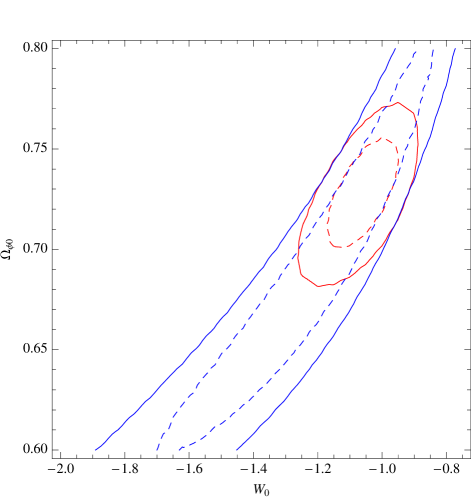
Figure 2: The $1-\sigma$ (solid) and $2-\sigma$ (dashed) contours in the plane defined by the present-day values of $\Omega_{\phi}$ and $w$ (denoted $\Omega_{\phi 0}$ and $w_{0}$ respectively) for the phantom ($w_{0}<-1$) or quintessence ($w_{0}>-1$) field, in the limit of a nearly flat potential. Blue (outer) contours are limits from SNIa alone. Red (inner) contours are SNIa+BAO.

We now compare the approximation given in equation (18) to exact numerical results. Kujat et al. KSS showed that phantom potentials with a negative kinetic term can be divided into three broad classes, depending on the late-time asymptotic behavior of $V^{\prime}(\phi)/V(\phi)$. When $V^{\prime}/V\rightarrow\pm\infty$ at late times, $w_{\phi}\rightarrow-\infty$. These models include, for instance, negative power laws. For models in which $V^{\prime}/V$ asymptotically approaches a constant, $w$ also approaches a constant, $w_{0}$, where $w_{0}<-1$. This class of models includes exponential potentials. Finally, when $V^{\prime}/V\rightarrow 0$ at late times, $w_{\phi}\rightarrow-1$. This class of models includes, for example, positive power law potentials. This final class of models, for which $w\rightarrow-1$, can be further subdivided into models which yield a future singularity (a “big rip”), and those which do not. The exact conditions necessary to avoid a big rip involve an integral function of $V(\phi)$ KSS , but for power-law potentials, the condition is simpler: for $V(\phi)=\phi^{\alpha}$, $\alpha>4$ yields a big rip, while $\alpha\leq 4$ yields no future singularity Sami ; KSS .

We have therefore chosen to compare our analytic approximation for $w(a)$ with a model from each of these four classes. The results are displayed in Fig. 1. As in the case of quintessence, the agreement between the actual evolution and our approximation in equation (18) is remarkably good, with the error in $w$ less than 0.5%. Our analytic approximation is well-fit by a linear relation, CPL

$$w(a)=w_{0}+w_{a}(1-a),$$ (19)

in the regime $a>0.5$, which corresponds to a redshift $z<1$. Further, for the value of $\Omega_{\phi 0}$ adopted here ($\Omega_{\phi 0}=0.7$), we have $w_{a}\approx-1.5(1+w_{0})$. This is the same relation between $w_{a}$ and $w_{0}$ noted empirically for linear quintessence potentials Kallosh , predicted for generic slow-roll quintessence models SS , and derived analytically for linear quintessence potentials Cahn . (Note that the latter reference gives a value of $-1.3$ rather than $-1.5$, but this difference is not significant, as the result depends on the assumed value of $\Omega_{\phi 0}$ and on the assumed definition of $w_{a}$; the latter is ambiguous since $w(a)$ is not exactly linear in $a$ in these models).

Given that equation (18) provides a generic prediction for the behavior of $w(a)$ in a wide class of phantom models, it is useful to compare this prediction to the observations. Further, since both quintessence and phantom models produce the same generic form for $w(a)$ in the limit where $V^{\prime}/V$ is small and nearly constant, we can combine the results for $w(a)$ for quintessence models from Ref. SS with the results for $w(a)$ for phantom models given here into a single likelihood plot. In Fig. 2, we compare this generic prediction for $w(a)$ to the SNIa and baryon acoustic oscillation data. The likelihoods were constructed using the 60 Essence supernovae, 57 SNLS (Supernova Legacy Survey) and 45 nearby supernovae, and the data release of 30 SNe Ia detected by HST and classified as the Gold sample by Riess et al. Riess . The combined dataset can be found in Ref. Davis . We also add the measurement of the baryon acoustic oscillation (BAO) scale at $z_{BAO}=0.35$ as observed by the Sloan Digital Sky Survey sdss .

It is important to note that Fig. 2 combines two completely different models. The portion of the figure with $w_{0}>-1$ corresponds to quintessence models, while $w_{0}<-1$ corresponds to phantom models. We have simply taken advantage of the fact that both models yield the same form for $w(a)$ as a function of $w_{0}$ and $\Omega_{\phi 0}$ in the limiting case where the potential is nearly flat.

Our main conclusion is that the analytic approximation previous derived for quintessence with a nearly flat potential SS has the same form when it is extended to phantom models with a negative kinetic term. Thus, the generic prediction for the evolution $w$ at low redshift ($z\lesssim 1$) in such models, $w(a)=w_{0}-1.5(1+w_{0})(1-a)$, can be applied to both $w_{0}>-1$ and $w_{0}<-1$.

- (1) R.A. Knop, et al., Ap.J. 598, 102 (2003).
- (2) J.L. Tonry, et al., Astrophys. J. 594, 1 (2003); B.J. Barris, et al., Astrophys. J. 602, 571 (2004); A.G. Riess, et al., Astrophys. J. 607, 665 (2004); P. Astier, et al, Astron. Astrophys. 447 31 (2006); A.G. Riess, et al., Astrophys. J. 659, 98 (2007).
- (3) E.J. Copeland, M. Sami, and S. Tsujikawa, Int. J. Mod. Phys. D 15, 1753 (2006).
- (4) W.M. Wood-Vasey, et al., Astrophys. J. 666, 694 (2007).
- (5) T.M. Davis, et al., Astrophys. J. 666, 716 (2007).
- (6) R.J. Scherrer and A.A. Sen, Phys. Rev. D77, 083515 (2008).
- (7) R. Crittenden, E. Majerotto, and F. Piazza, Phys. Rev. Lett. 98, 251301 (2007).
- (8) I.P. Neupane and C. Scherer, JCAP 0805, 009 (2008).
- (9) R.N. Cahn, R. de Putter, and E.V. Linder, arXiv:0807.1346.
- (10) R.R. Caldwell, Phys. Lett. B 545, 23 (2002).
- (11) R.R. Caldwell, M. Kamionkowski, and N.N. Weinberg, Phys. Rev. Lett. 91, 071301 (2003).
- (12) S. Nesseris and L. Perivolaropoulos, Phys. Rev. D70, 123529 (2004).
- (13) R.J. Scherrer, Phys. Rev. D71, 063519 (2005).
- (14) C.A. Egan and C.H. Lineweaver, arXiv:0712.3099.
- (15) S.M. Carroll, M. Hoffman, and M. Trodden, Phys. Rev. D68, 023509 (2003).
- (16) J.M. Cline, S. Jeon, and G.D. Moore, Phys. Rev. D70, 043543 (2004).
- (17) R.V. Buniy and S.D.H. Hsu, Phys. Lett. B 632, 543 (2006).
- (18) R.V. Buniy, S.D.H. Hsu, and B.M. Murray, hep-th/0606091.
- (19) Z.-K. Guo, Y.-S. Piao, and Y.-Z. Zhang, Phys. Lett. B 594, 247 (2004).
- (20) E. Elizalde, S. Nojiri, and S.D Odintsov, Phys. Rev. D70, 043539 (2004).
- (21) S. Nojiri and S.D. Odintsov, Phys. Rev. D70, 103522 (2004).
- (22) J.-G. Hao and X.-Z. Li, Phys. Rev. D70, 043529 (2004).
- (23) I. Ya. Aref’eva, A.S. Koshelev, and S. Yu. Vernov, astro-ph/0412619.
- (24) L. Perivolaropoulos, Phys. Rev. D71, 063503 (2005).
- (25) M. Sami, A. Toporensky, Mod. Phys. Lett. A 19, 1509 (2004).
- (26) V. Faraoni, Class. Quant. Grav. 22, 3235 (2005).
- (27) T. Chiba, Phys. Rev. D73, 063501 (2006).
- (28) J. Kujat, R.J. Scherrer, and A.A. Sen, Phys. Rev. D74, 083501 (2006).
- (29) P.J. Steinhardt, L. Wang, and I. Zlatev, Phys. Rev. D59, 123504 (1999).
- (30) M. Chevallier and D. Polarski, Int. J. Mod. Phys. D 10, 213 (2001); E.V. Linder, Phys. Rev. Lett. 90, 091301 (2003).
- (31) R. Kallosh, J. Kratochvil, A. Linde, E. V. Linder, and M. Shmakova, JCAP 0310, 015 (2003).
- (32) D.J. Eisenstein et al., Astrophys. J. 633, 560 (2005).