Multi-Particle Collision Dynamics — a Particle-Based Mesoscale Simulation Approach to the Hydrodynamics of Complex Fluids

In this review, we describe and analyze a mesoscale simulation method for fluid flow, which was introduced by Malevanets and Kapral in 1999, and is now called multi-particle collision dynamics (MPC) or stochastic rotation dynamics (SRD). The method consists of alternating streaming and collision steps in an ensemble of point particles. The multi-particle collisions are performed by grouping particles in collision cells, and mass, momentum, and energy are locally conserved. This simulation technique captures both full hydrodynamic interactions and thermal fluctuations. The first part of the review begins with a description of several widely used MPC algorithms and then discusses important features of the original SRD algorithm and frequently used variations. Two complementary approaches for deriving the hydrodynamic equations and evaluating the transport coefficients are reviewed. It is then shown how MPC algorithms can be generalized to model non-ideal fluids, and binary mixtures with a consolute point. The importance of angular-momentum conservation for systems like phase-separated liquids with different viscosities is discussed. The second part of the review describes a number of recent applications of MPC algorithms to study colloid and polymer dynamics, the behavior of vesicles and cells in hydrodynamic flows, and the dynamics of viscoelastic fluids.

PACS number(s): 47.11.-j, 05.40.-a, 02.70.Ns

1 Introduction

“Soft Matter” is a relatively new field of research that encompasses traditional complex fluids such as amphiphilic mixtures, colloidal suspensions, and polymer solutions, as well as a wide range of phenomena including chemically reactive flows (combustion), the fluid dynamics of self-propelled objects, and the visco-elastic behavior of networks in cells. One characteristic feature of all these systems is that phenomena of interest typically occur on mesoscopic length-scales—ranging from nano- to micrometers—and at energy scales comparable to the thermal energy $k_{B}T$.

Because of the complexity of these systems, simulations have played a particularly important role in soft matter research. These systems are challenging for conventional simulation techniques due to the presence of disparate time, length, and energy scales. Biological systems present additional challenges because they are often far from equilibrium and are driven by strong spatially and temporally varying forces. The modeling of these systems often requires the use of “coarse-grained” or mesoscopic approaches that mimic the behavior of atomistic systems on the length scales of interest. The goal is to incorporate the essential features of the microscopic physics in models which are computationally efficient and are easily implemented in complex geometries and on parallel computers, and can be used to predict behavior, test physical theories, and provide feedback for the design and analysis of experiments and industrial applications.

In many situations, a simple continuum description based on the Navier-Stokes equation is not sufficient, since molecular-level details—including thermal fluctuations—play a central role in determining the dynamic behavior. A key issue is to resolve the interplay between thermal fluctuations, hydrodynamic interactions, and spatio-temporally varying forces. One well-known example of such systems are microemulsions—a dynamic bicontinuous network of intertwined mesoscopic patches of oil and water—where thermal fluctuations play a central role in creating this phase. Other examples include flexible polymers in solution, where the coil state and stretching elasticity are due to the large configurational entropy. On the other hand, atomistic molecular dynamics simulations retain too many microscopic degrees of freedom, consequently requiring very small time steps in order to resolve the high frequency modes. This makes it impossible to study long timescale behavior such as self-assembly and other mesoscale phenomena.

In order to overcome these difficulties, considerable effort has been devoted to the development of mesoscale simulation methods such as Dissipative Particle Dynamics hoog_92_smh ; espa_95_hfd ; espa_95_fk , Lattice-Boltzmann mcna_88_ube ; shan_93_lbm ; he_97_tlb , and Direct Simulation Monte Carlo bird_94_mgd ; alex_97_dsm ; garc_00_nmp . The common approach of all these methods is to “average out” irrelevant microscopic details in order to achieve high computational efficiency while keeping the essential features of the microscopic physics on the length scales of interest. Applying these ideas to suspensions leads to a simplified, coarse-grained description of the solvent degrees of freedom, in which embedded macromolecules such as polymers are treated by conventional molecular dynamics simulations.

All these approaches are essentially alternative ways of solving the Navier-Stokes equation and its generalizations. This is because the hydrodynamic equations are expressions for the local conservation laws of mass, momentum, and energy, complemented by constitutive relations which reflect some aspects of the microscopic details. Frisch et al. fris_86_lan demonstrated that discrete algorithms can be constructed which recover the Navier-Stokes equation in the continuum limit as long as these conservation laws are obeyed and space is discretized in a sufficiently symmetric manner.

The first model of this type was a cellular automaton, called the Lattice-Gas-Automaton (LG). The algorithm consists of particles which jump between nodes of a regular lattice at discrete time intervals. Collisions occur when more than one particle jumps to the same node, and collision rules are chosen which impose mass and momentum conservation. The Lattice-Boltzmann method (LB)—which follows the evolution of the single-particle probability distribution at each node—was a natural generalization of this approach. LB solves the Boltzmann equation on a lattice with a small set of discrete velocities determined by the lattice structure. The price for obtaining this efficiency is numerical instabilities in certain parameter ranges. Furthermore, as originally formulated, LB did not contain any thermal fluctuations. It became clear only very recently (and only for simple liquids) how to restore fluctuations by introducing additional noise terms to the algorithm adhi_05_flb .

Except for conservation laws and symmetry requirements, there are relatively few constraints on the structure of mesoscale algorithms. However, the constitutive relations and the transport coefficients depend on the details of the algorithm, so that the temperature and density dependencies of the transport coefficients can be quite different from those of real gases or liquids. However, this is not a problem as long as the functional form of the resulting hydrodynamic equations is correct. The mapping to real systems is achieved by tuning the relevant characteristic numbers, such as the Reynolds and Peclet numbers dhon96 ; lars_99_src , to those of a given experiment. When it is not possible to match all characteristic numbers, one concentrates on those which are of order unity, since this indicates that there is a delicate balance between two effects which need to be reproduced by the simulation. On occasion, this can be difficult, since changing one internal parameter, such as the mean free path, usually affects all transport coefficients in different ways, and it may happen that a given mesoscale algorithm is not at all suited for a given application ripo_04_lhc ; ripo_05_drf ; hecht_05_scc ; padd_06_hib .

In this review we focus on the development and application of a particle-based mesoscopic simulation technique which was recently introduced by Malevanets and Kapral male_99_mms ; male_00_smd . The algorithm, which consists of discrete streaming and collision steps, shares many features with Bird’s Direct Simulation Monte Carlo (DSMC) approach bird_94_mgd . Collisions occur at fixed discrete time intervals, and although space is discretized into cells to define the multi-particle collision environment, both the spatial coordinates and the velocities of the particles are continuous variables. Because of this, the algorithm exhibits unconditional numerical stability and has an $H$-theorem male_99_mms ; ihle_03_srd_a . In this review, we will use the name multi-particle collision dynamics (MPC) to refer to this class of algorithms. In the original and most widely used version of MPC, collisions consist of a stochastic rotation of the relative velocities of the particles in a collision cell. We will refer to this algorithm as stochastic rotation dynamics (SRD) in the following.

One important feature of MPC algorithms is that the dynamics is well-defined for an arbitrary time step, $\Delta t$. In contrast to methods such as molecular dynamics simulations (MD) or dissipative particle dynamics (DPD), which approximate the continuous-time dynamics of a system, the time step does not have to be small. MPC defines a discrete-time dynamics which has been shown to yield the correct long-time hydrodynamics; one consequence of the discrete dynamics is that the transport coefficients depend explicitly on $\Delta t$. In fact, this freedom can be used to tune the Schmidt number, $Sc$ ripo_05_drf ; keeping all other parameters fixed, decreasing $\Delta t$ leads to an increase in $Sc$. For small time steps, $Sc$ is larger than unity (as in a dense fluid), while for large time steps, $Sc$ is of order unity, as in a gas.

Because of its simplicity, SRD can be considered an “Ising model” for hydrodynamics, since it is Galilean invariant (when a random grid shift of the collision cells is performed before each collision step ihle_01_srd ) and incorporates all the essential dynamical properties in an algorithm which is remarkably easy to analyze. In addition to the conservation of momentum and mass, SRD also locally conserves energy, which enables simulations in the microcanonical ensemble. It also fully incorporates both thermal fluctuations and hydrodynamic interactions. Other more established methods, such as Brownian Dynamics (BD) can also be augmented to include hydrodynamic interactions. However, the additional computational costs are often prohibitive mohan_07_utp ; kim_06_bdf . In addition, hydrodynamic interactions can be easily switched off in MPC algorithms, making it easy to study the importance of hydrodynamic interactions kiku_02_pcp ; ripo_07_hss .

It must, however, be emphasized that all local algorithms such as MPC, DPD, and LB model compressible fluids, so that it takes time for the hydrodynamic interactions to “propagate” over longer distances. As a consequence, these methods become quite inefficient in the Stokes limit, where the Reynolds number approaches zero. Algorithms which incorporate an Oseen tensor do not share this shortcoming.

The simplicity of the SRD algorithm has made it possible to derive analytic expressions for the transport coefficients which are valid for both large and small mean free paths kiku_03_tcm ; ihle_03_srd_b ; ihle_05_ect . This is usually very difficult to do for other mesoscale particle-based algorithms. Take DPD as an example: the viscosity measured in Ref. backer_05_pf is about $50\%$ smaller than the value predicted theoretically in the same paper. For SRD, the agreement is generally better than $1\%$.

MPC is particularly well suited for (i) studying phenomena where both thermal fluctuations and hydrodynamics are important, (ii) for systems with Reynolds and Peclet numbers of order $0.1$ to $10$, (iii) if exact analytical expressions for the transport coefficients and consistent thermodynamics are needed, and (iv) for modeling complex phenomena for which the constitutive relations are not known. Examples include chemically reacting flows, self-propelled objects, or solutions with embedded macromolecules and aggregates.

If thermal fluctuations are not essential or undesirable, a more traditional method such as a finite-element solver or a Lattice-Boltzmann approach is recommended. If, on the other hand, inertia and fully resolved hydrodynamics are not crucial, but fluctuations are, one might be better served using Langevin or Brownian Dynamics.

This review consists of two parts. The first part begins with a description of several widely used MPC algorithms in Sec. 2, and then discusses important features of the original SRD algorithm and a frequently used variation (MPC-AT), which effectively thermostats the system by replacing the relative velocities of particles in a collision cell with newly generated Gaussian random numbers in the collision step. After a qualitative discussion of the static and dynamic properties of MPC fluids in Sec. 3, two alternative approaches for deriving the hydrodynamic equations and evaluating the transport coefficients are described. First, in Sec. 4, discrete-time projection operator methods are discussed and the explicit form of the resulting Green-Kubo relations for the transport coefficients are given and evaluated. Subsequently, in Sec. 5, an alternative non-equilibrium approach is described. The two approaches complement each other, and the predictions of both methods are shown to be in complete agreement. It is then shown in Sec. 6 how MPC algorithms can be generalized to model non-ideal fluids and binary mixtures, Finally, various approaches for implementing slip and no-slip boundary conditions—as well as the coupling of embedded objects to a MPC solvent—are described in Sec. 7. In Sec. 8, the importance of angular-momentum conservation is discussed, in particular in systems of phase-separated fluids with different viscosities under flow. An important aspect of mesoscale simulations is the possibility to directly assert the effect of hydrodynamic interactions by switching them off, while retaining the same thermal fluctuations and similar friction coefficients; in MPC, this can be done very efficiently by an algorithm described in Sec. 9. The second part of the review describes a number of recent applications of MPC algorithms to study colloid and polymer dynamics, and the behavior of vesicles and cells in hydrodynamic flows. Sec. 10 focuses on the non-equilibrium behavior of colloidal suspensions, the dynamics of dilute solutions of linear polymers both in equilibrium and under flow conditions, and the properties of star polymers—also called ultra-soft colloids—in shear flow. Sec. 11 is devoted to the review of recent simulation results for membranes in flow. After a short introduction to the modeling of membranes with different levels of coarse-graining, the behavior of fluid vesicles and red blood cells, both in shear and capillary flow, is discussed. Finally, a simple extension of MPC for viscoelastic solvents is described in Sec. 12, where the point particles of MPC for Newtonian fluids are replaced by harmonic dumbbells.

A discussion of several complementary applications—such as chemically reactive flows and self-propelled objects—can be found in a recent review of MPC by R. Kapral kapr_08_mpc .

2 Algorithms

In the following, we use the term multi-particle collision dynamics (MPC) to describe the generic class of particle-based algorithms for fluid flow which consist of successive free-streaming and multi-particle collision steps. The name stochastic rotation dynamics (SRD) is reserved for the most widely used algorithm which was introduced by Malevanets and Kapral male_99_mms . The name refers to the fact that the collisions consist of a random rotation of the relative velocities $\delta{\bf v}_{i}={\bf v}_{i}-{\bf u}$ of the particles in a collision cell, where ${\bf u}$ is the mean velocity of all particles in a cell. There are a number of other MPC algorithms with different collision rules alla_02_mss ; nogu_07_pmh ; ihle_06_cpa . For example, one class of algorithms uses modified collision rules which provide a nontrivial “collisional” contribution to the equation of state ihle_06_cpa ; tuzel_06_ctc . As a result, these models can be used to model non-ideal fluids or multi-component mixtures with a consolute point.

2.1 Stochastic Rotation Dynamics (SRD)

In SRD, the solvent is modeled by a large number $N$ of point-like particles of mass $m$ which move in continuous space with a continuous distribution of velocities. The algorithm consists of individual streaming and collision steps. In the streaming step, the coordinates, ${\bf r}_{i}(t)$, of all solvent particles at time $t$ are simultaneously updated according to

$${\bf r}_{i}(t+\Delta t)={\bf r}_{i}(t)+\Delta t\,{\bf v}_{i}(t)\,,$$ (1)

where ${\bf v}_{i}(t)$ is the velocity of particle $i$ at time $t$ and $\Delta t$ is the value of the discretized time step.

In order to define the collisions, particles are sorted into cells, and they interact only with members of their own cell. Typically, the system is coarse-grained into cells of a regular, typically cubic, grid with lattice constant $a$. In practice, lengths are often measured in units of $a$, which corresponds to setting $a=1$. The average number of particles per cell, $M$, is typically chosen to be between three and 20. The actual number of particles in cell at a given time, which fluctuates, will be denoted by $N_{c}$. The collision step consists of a random rotation R of the relative velocities $\delta{\bf v}_{i}={\bf v}_{i}-{\bf u}$ of all the particles in the collision cell,

$${\bf v}_{i}(t+\Delta t)={\bf u}(t)+{\bf R}\cdot\delta{\bf v}_{i}(t)\,.$$ (2)

All particles in the cell are subject to the same rotation, but the rotations in different cells and at different times are statistically independent. There is a great deal of freedom in how the rotation step is implemented, and any stochastic rotation matrix which satisfies semi-detailed balance can be used. Here, we describe the most commonly used algorithm. In two dimensions, ${\bf R}$ is a rotation by an angle $\pm\alpha$, with probability $1/2$. In three dimensions, a rotation by a fixed angle $\alpha$ about a randomly chosen axis is typically used. Note that rotations by an angle $-\alpha$ need not be considered, since this amounts to a rotation by an angle $\alpha$ about an axis with the opposite orientation. If we denote the randomly chosen rotation axis by $\hat{\bf R}$, the explicit collision rule in three dimensions is

$${\bf v}_{i}(t+\Delta t)={\bf u}(t) + \delta{\bf v}_{i,\perp}(t)\cos(\alpha)$$ (3)

$$+ (\delta{\bf v}_{i,\perp}(t)\times\hat{\bf R})\sin(\alpha)+\delta{\bf v}_{i,\|}(t)\,,$$

where $\perp$ and $\|$ are the components of the vector which are perpendicular and parallel to the random axis $\hat{\bf R}$, respectively. Malevanets and Kapral male_99_mms have shown that there is an $H$-theorem for the algorithm, that the equilibrium distribution of velocities is Maxwellian, and that it yields the correct hydrodynamic equations with an ideal-gas equation of state.

In its original form male_99_mms ; male_00_smd , the SRD algorithm was not Galilean invariant. This is most pronounced at low temperatures or small time steps, where the mean free path, $\lambda=\Delta t\sqrt{k_{B}T/m}$, is smaller than the cell size $a$. If the particles travel a distance between collisions which is small compared to the cell size, essentially the same particles collide repeatedly before other particles enter the cell or some of the participating particles leave the cell. For small $\lambda$, large numbers of particles in a given cell remain correlated over several time steps. This leads to a breakdown of the molecular chaos assumption—i.e., particles become correlated and retain information of previous encounters. Since these correlations are changed by a homogeneous imposed flow field, ${\bf V}$, Galilean invariance is destroyed, and the transport coefficients depend on both the magnitude and direction of ${\bf V}$.

Ihle and Kroll ihle_01_srd ; ihle_03_srd_a showed that Galilean invariance can be restored by performing a random shift of the entire computational grid before every collision step. The grid shift constantly groups particles into new collision neighborhoods; the collision environment no longer depends on the magnitude of an imposed homogeneous flow field, and the resulting hydrodynamic equations are Galilean invariant for arbitrary temperatures and Mach number. This procedure is implemented by shifting all particles by the same random vector with components uniformly distributed in the interval $[-a/2,a/2]$ before the collision step. Particles are then shifted back to their original positions after the collision.

In addition to restoring Galilean invariance, this grid-shift procedure accelerates momentum transfer between cells and leads to a collisional contribution to the transport coefficients. If the mean free path $\lambda$ is larger than $a/2$, the violation of Galilean invariance without grid shift is negligible, and it is not necessary to use this procedure.

2.1.1 SRD with Angular Momentum Conservation

As noted by Pooley and Yeomans pool_05_ktd and confirmed in Ref. ihle_05_ect , the macroscopic stress tensor of SRD is not symmetric in $\partial_{\alpha}v_{\beta}$. The reason for this is that the multi-particle collisions do not, in general, conserve angular momentum. The problem is particularly pronounced for small mean free paths, where asymmetric collisional contributions to the stress tensor dominate the viscosity (see Sec. 4.1.1). In contrast, for mean free paths larger than the cell size, where kinetic contributions dominate, the effect is negligible.

An anisotropic stress tensor means that there is non-zero dissipation if the entire fluid undergoes a rigid-body rotation, which is clearly unphysical. However, as emphasized in Ref. ihle_05_ect , this asymmetry is not a problem for most applications in the incompressible (or small Mach number) limit, since the form of the Navier-Stokes equation is not changed. This is in accordance with results obtained in SRD simulations of vortex shedding behind an obstacle lamu_01_mcd , and vesicle nogu_04_fvv and polymer dynamics ripo_04_lhc . In particular, it has been shown that the linearized hydrodynamic modes are completely unaffected in two dimensions; in three dimensions only the sound damping is slightly modified ihle_05_ect .

However, very recently Götze et al. gotz_07_ram identified several situations involving rotating flow fields in which this asymmetry leads to significant deviations from the behavior of a Newtonian fluid. This includes (i) systems in which boundary conditions are defined by torques rather than prescribed velocities, (ii) mixtures of liquids with a viscosity contrast, and (iii) polymers with a locally high monomer density and a monomer-monomer distance on the order of or smaller than the lattice constant, $a$, embedded in a MPC fluid. A more detailed discussion will be presented in Sec. 8 below.

For the SRD algorithm, it is possible to restore angular momentum conservation by having the collision angle depend on the specific positions of the particles within a collision cell. Such a modification was first suggested by Ryder ryde_05_the for SRD in two dimensions. She showed that the angular momentum of the particles in a collision cell is conserved if the collision angle $\alpha$ is chosen such that

$${\rm sin}(\alpha)=-2AB/(A^{2}+B^{2})\,\,\,{\rm and}\,\,\,{\rm cos}(\alpha)=(A^{2}-B^{2})/(A^{2}+B^{2})$$ (4)

where

$$A=\sum_{1}^{N_{c}}\,[{\bf r}_{i}\times({\bf v}_{i}-{\bf u})]|_{z}\ \ \ {\rm and}\ \ \ B=\sum_{1}^{N_{c}}\,{\bf r}_{i}\cdot({\bf v}_{i}-{\bf u}).$$ (5)

When the collision angles are determined in this way, the viscous stress tensor is symmetric. Note, however, that evaluating Eq. (4) is time-consuming, since the collision angle needs to be computed for every collision cell every time step. This typically increases the CPU time by a factor close to two.

A general procedure for implementing angular-momentum conservation in multi-particle collision algorithms was introduced by Noguchi et al. nogu_07_pmh ; it is discussed in the following section.

2.2 Multi-Particle Collision Dynamics with Anderson Thermostat (MPC-AT)

A stochastic rotation of the particle velocities relative to the center-of-mass velocity is not the only possibility for performing multi-particle collisions. In particular, MPC simulations can be performed directly in the canonical ensemble by employing an Anderson thermostat (AT) alla_02_mss ; nogu_07_pmh ; the resulting algorithm will be referred to as MPC-AT-a. In this algorithm, instead of performing a rotation of the relative velocities, $\{\delta{\bf v}_{i}\}$, in the collision step, new relative velocities are generated. The components of $\{\delta{\bf v}^{ran}_{i}\}$ are Gaussian random numbers with variance $\sqrt{k_{B}T/m}$. The collision rule is nogu_07_pmh ; gotz_07_ram

$${\bf v}_{i}(t+\Delta t)={\bf u}(t)+\delta{\bf v}_{i}^{ran}={\bf u}(t)+{\bf v}_{i}^{ran}-\sum_{j\in cell}{\bf v}_{j}^{ran}/N_{c}\,,$$ (6)

where $N_{c}$ is the number of particles in the collision cell, and the sum runs over all particles in the cell. It is important to note that MPC-AT is both a collision procedure and a thermostat. Simulations are performed in the canonical ensemble, and no additional velocity rescaling is required in non-equilibrium simulations, where there is viscous heating.

Just as SRD, this algorithm conserves momentum at the cell level but not angular momentum. Angular momentum conservation can be restored ryde_05_the ; nogu_07_pmh by imposing constraints on the new relative velocities. This leads to an angular-momentum conserving modification of MPC-AT gotz_07_ram ; nogu_07_pmh , denoted MPC-AT$+a$. The collision rule in this case is

$${\bf v}_{i}(t+\Delta t) = {\bf u}(t)+{\bf v}_{i,ran}-\sum_{cell}{\bf v}_{i,ran}/N_{c}$$ (7)

$$+\left\{m\mbox{\boldmath$\Pi$}^{-1}\sum_{j\in cell}\left[{\bf r}_{j,c}\times({\bf v}_{j}-{\bf v}_{j}^{ran})\right]\times{\bf r}_{i,c}\right\},$$

where $\Pi$ is the moment of inertia tensor of the particles in the cell, and ${\bf r}_{i,c}={\bf r}_{i}-{\bf R}_{c}$ is the relative position of particle $i$ in the cell and ${\bf R}_{c}$ is the center of mass of all particles in the cell.

When implementing this algorithm, an unbiased multi-particle collision is first performed, which typically leads to a small change of angular momentum, $\Delta\vec{L}$. By solving the linear equation $-\Delta\vec{L}=\bf{\Pi}\cdot\vec{\omega}$, the angular velocity $\omega$ which is needed to cancel the initial change of angular momentum is then determined. The last term in Eq. (7) restores this angular momentum deficiency. MPC-AT can be adapted for simulations in the micro-canonical ensemble by imposing an additional constraint on the values of the new random relative velocities nogu_07_pmh .

2.2.1 Comparison of SRD and MPC-AT

Because $d$ Gaussian random numbers per particle are required at every iteration, where $d$ is the spatial dimension, the speed of the random number generator is the limiting factor for MPC-AT. In contrast, the efficiency of SRD is rather insensitive to the speed of the random number generator since only $d-1$ uniformly distributed random numbers are needed in every box per iteration, and even a low quality random number generator is sufficient, because the dynamics is self-averaging. A comparison for two-dimensional systems shows that MPC-AT-a is about a factor 2 to 3 times slower than SRD, and that MPC-AT+a is about a factor 1.3 to 1.5 slower than MPC-AT-a goetz_private .

One important difference between SRD and MPC-AT is the fact that relaxation times in MPC-AT generally decrease when the number of particles per cell is increased, while they increase for SRD. A longer relaxation time means that a larger number of time steps is required for transport coefficients to reach their asymptotic value. This could be of importance when fast oscillatory or transient processes are investigated. As a consequence, when using SRD, the average number of particles per cell should be in range of $3-20$; otherwise, the internal relaxation times could be no longer negligible compared to physical time scales. No such limitation exists for MPC-AT, where the relaxation times scale as $(\ln M)^{-1}$, where $M$ is the average number of particles in a collision cell.

2.3 Computationally Efficient Cell-Level Thermostating for SRD

The MPC-AT algorithm discussed in Sec. 2.2 provides a very efficient particle-level thermostating of the system. However, it is considerably slower than the original SRD algorithm, and there are situations in which the additional freedom offered by the choice of SRD collision angle can be useful.

Thermostating is required in any non-equilibrium MPC simulation, where there is viscous heating. A basic requirement of any thermostat is that it does not violate local momentum conservation, smear out local flow profiles, or distort the velocity distribution too much. When there is homogeneous heating, the simplest way to maintain a constant temperature is to just rescale velocity components by a scale factor $S$, $v^{new}_{\alpha}=Sv_{\alpha}$, which adjusts the total kinetic energy to the desired value. This can be done with just a single global scale factor, or a local factor which is different in every cell. For a known macroscopic flow profile, ${\bf u}$, like in shear flow, the relative velocities ${\bf v}-{\bf u}$ can be rescaled. This is known as a profile-unbiased thermostat; however, it has been shown to have deficiencies in molecular dynamics simulations erpe_84_svh .

Here we describe an alternative thermostat which exactly conserves momentum in every cell and is easily incorporated into the MPC collision step. It was originally developed by Heyes for constant-temperature molecular dynamics simulations; however, the original algorithm described in Ref. alle:87 violates detailed balance. The thermostat consists of the following procedure which is performed independently in every collision cell as part of the collision step.

1. Randomly select a real number $\psi\in[1,1+c]$, where $c$ is a small number between 0.05 and 0.3 which determines the strength of the thermostat.

2. Accept this number as a scaling factor $S=\psi$ with probability $1/2$; otherwise, take $S=1/\psi$.

3. Create another random number $\xi\in[0,1]$. Rescale the velocities if $\xi$ is smaller than the acceptance probability $p_{A}=\min(1,A)$, where

   $$A=S^{d\,(N_{c}-1)}{\rm exp}\left(-\frac{m}{2k_{B}T_{0}}\,\sum_{i=1}^{N_{c}}\,({\bf v}_{i}-{\bf u})^{2}\{S^{2}-1\}\right).$$ (8)

   $d$ is the spatial dimension, and $N_{c}$ is the number of particles in the cell. The prefactor in Eq. (8) is an entropic contribution which accounts for the fact that the phase-space volume changes if the velocities are rescaled.

4. If the attempt is accepted, perform a stochastic rotation with the scaled rotation matrix $S\,{\bf R}$. Otherwise, use the rotation matrix ${\bf R}$.

This thermostat reproduces the Maxwell velocity distribution and does not change the viscosity of the fluid. It gives excellent equilibration, and the deviation of the measured kinetic temperature from $T_{0}$ is smaller than $0.01\%$. The parameter $c$ controls the rate at which the kinetic temperature relaxes to $T_{0}$, and in agreement with experience from MC-simulations, an acceptance rate in the range of $50\%$ to $65\%$ leads to the fastest relaxation. For these acceptance rates, the relaxation time is of order $5-10$ time steps. The corresponding value for $c$ depends on the particle number $N_{c}$; in two dimensions, it is about $0.3$ for $N_{c}=7$ and decreases to $0.05$ for $N_{c}=100$. This thermostat has been successfully applied to SRD simulations of sedimenting charged colloids hecht_05_scc .

3 Qualitative Discussion of Static and Dynamic Properties

The previous section outlines several multi-particle algorithms. A detailed discussion of the link between the microscopic dynamics described by Eqs. (1) and (2) or (3) and the macroscopic hydrodynamic equations, which describe the behavior at large length and time scales, requires a more careful analysis of the corresponding Liouville operator ${\cal L}$. Before describing this approach in more detail, we provide a more heuristic discussion of the equation of state and of one of the transport coefficients, the shear viscosity, using more familiar approaches for analyzing the behavior of dynamical systems.

3.1 Equation of State

In a homogeneous fluid, the pressure is the normal force exerted by the fluid on one side of a unit area on the fluid on the other side; expressed somewhat differently, it is the momentum transfer per unit area per unit time across an imaginary (flat) fixed surface. There are both kinetic and virial contributions to the pressure. The first arises from the momentum transported across the surface by particles that cross the surface in the unit time interval; it yields the ideal-gas contribution, $P_{id}=Nk_{B}T/V$, to the pressure. For classical particles interacting via pair-additive, central forces, the intermolecular “potential” contribution to the pressure can be determined using the method introduced by Irving and Kirkwood irvi_50_smt . A clear discussion of this approach is given by Davis in Ref. davi_96_smp , where it is shown to lead to the virial equation of state of a homogeneous fluid,

$$P=\frac{Nk_{B}T}{V}+\frac{1}{3V}\sum_{i}\langle{\bf r}_{i}\cdot{\bf F}_{i}\rangle,$$ (9)

in three dimensions, where ${\bf F}_{i}$ is the force on particle $i$ due to all the other particles, and the sum runs over all particles of the system.

The kinetic contribution to the pressure, $P_{id}=Nk_{B}T/V$, is clearly present in all MPC algorithms. For SRD, this is the only contribution. The reason is that the stochastic rotations, which define the collisions, transport (on average) no net momentum across a fixed dividing surface. More general MPC algorithms (such as those discussed in Sec. 6) have an additional contribution to the virial equation of state. However, instead of an explicit force ${\bf F}_{i}$ as in Eq. (9), the contribution from the multi-particle collisions is a force of the form $m\Delta v_{i}/\Delta t$, and the role of the particle position, ${\bf r}_{i}$, is played by a variable which denotes the cell-partners which participate in the collision ihle_06_cpa ; tuze_07_mmf .

3.2 Shear Viscosity

Just as for the pressure, there are both kinetic and collisional contributions to the transport coefficients. We present here a heuristic discussion of these contributions to the shear viscosity, since it illustrates rather clearly the essential physics and provides background for subsequent technical discussions.

Consider a reference plane (a line in two dimensions) with normal in the $y$-direction embedded in a homogeneous fluid in equilibrium. The fluid below the plane exerts a mean force ${\bf p}_{y}$ per unit area on the fluid above the plane; by Newton’s third law, the fluid above the plane must exert a mean force $-{\bf p}_{y}$ on the fluid below the plane. The normal force per unit area is just the mean pressure, $P$, so that $p_{yy}=P$. In a homogeneous simple fluid in which there are no velocity gradients, there is no tangential force, so that, for example, $p_{yx}=0$. $p_{\alpha\beta}$ is called the pressure tensor, and the last result is just a statement of the well known fact that the pressure tensor in a homogeneous simple fluid at equilibrium has no off-diagonal elements; the diagonal elements are all equal to the mean pressure $P$.

Consider a shear flow with a shear rate $\dot{\gamma}=\partial u_{x}(y)/\partial y$. In this case, there is a tangential stress on the reference surface because of the velocity gradient normal to the plane. In the small gradient limit, the dynamic viscosity, $\eta$, is defined as the coefficient of proportionality between the tangential stress, $p_{yx}$, and the normal gradient of the imposed velocity gradient,

$$p_{yx}=-\eta\dot{\gamma}.$$ (10)

The kinematic viscosity, $\nu$, is related to $\eta$ by $\nu=\eta/\rho$, where $\rho=nm$ is the mass density, with $n$ the number density of the fluid and $m$ the particle mass.

Kinetic contribution to the shear viscosity: The kinetic contribution to the shear viscosity comes from transverse momentum transport by the flow of fluid particles. This is the dominant contribution to the viscosity of gases. The following analogy may make this origin of viscosity clearer. Consider two ships moving side by side in parallel, but with different speeds. If the sailors on the two ships constantly throw sand bags from their ship onto the other, there will be a transfer of momentum between to two ships so that the slower ship accelerates and the faster ship decelerates. This can be interpreted as an effective friction, or kinetic viscosity, between the ships. There are no direct forces between the ships, and the transverse momentum transfer originates solely from throwing sandbags from one ship to the other.

A standard result from kinetic theory is that the kinetic contribution to the shear viscosity in simple gases is reif_65

$$\eta^{kin}\sim nm\bar{v}\lambda,$$ (11)

where $\lambda$ is the mean free path and $\bar{v}$ is the thermal velocity. Using the fact that $\lambda\sim\bar{v}\Delta t$ for SRD and that $\bar{v}\sim\sqrt{k_{B}T/m}$, relation (11) implies that

$$\eta^{kin}\sim nk_{B}T\Delta t,\ \ \ \ {\rm or\ equivalently,}\ \ \ \ \nu^{kin}\sim k_{B}T\Delta t/m,$$ (12)

which is, as more detailed calculations presented later will show, the correct dependence on $n$, $k_{B}T$, and $\Delta t$. In fact, the general form for the kinetic contribution to the kinematic viscosity is

$$\nu^{kin}=\frac{k_{B}T\Delta t}{m}f_{kin}(d,M,\alpha),$$ (13)

where $d$ is the spatial dimension, $M$ is the mean number of particles per cell, and $\alpha$ is the SRD collision angle. Another way of obtaining this result is to use the analogy with a random walk: The kinematic viscosity is the diffusion coefficient for momentum diffusion. At large mean free path, $\lambda/a\gg 1$, momentum is primarily transported by particle translation (as in the ship analogy). The mean distance a particle streams during one time step, $\Delta t$, is $\lambda$. According to the theory of random walks, the corresponding diffusion coefficient scales as $\nu^{kin}\sim\lambda^{2}/\Delta t\sim k_{B}T\Delta t/m$.

Note that in contrast to a “real” gas, for which the viscosity has a square root dependence on the temperature, $\nu^{kin}\sim T$ for SRD. This is because the mean free path of a particle in SRD does not depend on density; SRD allows particles to stream right through each other between collisions. Note, however, that SRD can be easily modified to give whatever temperature dependence is desired. For example, an additional temperature-dependent collision probability can be introduced; this would be of interest, e.g., for a simulation of realistic shock-wave profiles.

Collisional contribution to the shear viscosity: At small mean free paths, $\lambda/a\ll 1$, particles “stream” only a short distance between collisions, and the multi-particle “collisions” are the primary mechanism for momentum transport. These collisions redistribute momenta within cells of linear size $a$. This means that momentum “hops” an average distance $a$ in one time step, leading to a momentum diffusion coefficient $\nu^{col}\sim a^{2}/\Delta t$. The general form of the collisional contribution to the shear viscosity is therefore

$$\nu^{col}=\frac{a^{2}}{\Delta t}f_{col}(d,M,\alpha).$$ (14)

This is indeed the scaling observed in numerical simulations at small mean free path.

The kinetic contribution dominates for $\lambda\gg a$, while the collisional contribution dominates in the opposite limit. Two other transport coefficients of interest are the thermal diffusivity, $D_{T}$, and the single particle diffusion coefficient, $D$. Both have the dimension m²/sec. As dimensional analysis would suggest, the kinetic and collisional contributions to $D_{T}$ exhibit the same characteristic dependencies on $\lambda$, $a$, and $\Delta t$ described by Eqs. (13) and (14). Since there is no collisional contribution to the diffusion coefficient, $D\sim\lambda^{2}/\Delta t$.

Two complementary approaches have been used to derive the transport coefficients of the SRD fluid. The first is an equilibrium approach which utilizes a discrete projection operator formalism to obtain Green-Kubo (GK) relations which express the transport coefficients as sums over the autocorrelation functions of reduced fluxes. This approach was first utilized by Malevanets and Kapral male_00_smd , and later extended by Ihle, Kroll and Tüzel ihle_03_srd_a ; ihle_03_srd_b ; ihle_05_ect to include collisional contributions and arbitrary rotation angles. This approach is described in Sec. 4.1.

The other approach uses kinetic theory to calculate the transport coefficients in stationary non-equilibrium situation such as shear flow. The first application of this approach to SRD was presented in Ref. ihle_01_srd , where the collisional contribution to the shear viscosity for large $M$, where particle number fluctuations can be ignored, was calculated. This scheme was later extended by Kikuchi et al. kiku_03_tcm to include fluctuations in the number of particles per cell, and then used to obtain expressions for the kinetic contributions to shear viscosity and thermal conductivity pool_05_ktd . This non-equilibrium approach is described in Sec. 5.

4 Equilibrium Calculation of Dynamic Properties

A projection operator formalism for deriving the linearized hydrodynamic equations and Green-Kubo (GK) relations for the transport coefficients of molecular fluids was originally introduced by Zwanzig zwan_61_ltp ; mori_65_tcm ; mori_65_crt and later adapted for lattice gases by Dufty and Ernst duft_89_grl . With the help of this formalism, explicit expressions for both the reversible (Euler) as well as dissipative terms of the long-time, large-length-scale hydrodynamics equations for the coarse-grained hydrodynamic variables were derived. In addition, the resulting GK relations enable explicit calculations of the transport coefficients of the fluid. This work is summarized in Sec. 4.1. An analysis of the equilibrium fluctuations of the hydrodynamic modes can then be used to directly measure the shear and bulk viscosities as well as the thermal diffusivity. This approach is described in Sec. 4.2, where SRD results for the dynamic structure factor are discussed.

4.1 Linearized Hydrodynamics and Green-Kubo Relations

The Green-Kubo (GK) relations for SRD differ from the well-known continuous versions due to the discrete-time dynamics, the underlying lattice structure, and the multi-particle interactions. In the following, we briefly outline this approach for determining the transport coefficients. More details can be found in Refs. ihle_03_srd_a ; ihle_03_srd_b .

The starting point of this theory are microscopic definitions of local hydrodynamic densities $A_{\beta}$. These “slow” variables are the local number, momentum, and energy density. At the cell level, they are defined as

$$A_{\beta}(\mbox{\boldmath$\xi$})=\sum_{i=1}^{N}a_{\beta,i}\prod_{\gamma=1}^{d}\Theta\left({a\over 2}-\left|\xi_{\gamma}+{a\over 2}-r_{i\gamma}\right|\right),$$ (15)

with the discrete cell coordinates $\mbox{\boldmath$\xi$}=a{\bf m}$, where $m_{\beta}=1,\dots,L$, for each spatial component. $a_{1,i}=1$ is the particle density, $\{a_{\beta,i}\}=m\{v_{i(\beta-1)}\}$, with $\beta=2,...,d+1$, are the components of the particle momenta, and $a_{d+2,i}=mv_{i}^{2}/2$ is the kinetic energy of particle $i$. $d$ is the spatial dimension, and ${\bf r}_{i}$ and ${\bf v}_{i}$ are position and velocity of particle $i$, respectively.

$A_{\beta}(\mbox{\boldmath$\xi$})$, for $\beta=2,\dots,d+2$, are cell level coarse-grained densities. For example, $A_{2}(\mbox{\boldmath$\xi$})$ is the $x$-component of the total momentum of all the particles in cell $\xi$ at the given time. Note that the particle density, $A_{1}$, was not coarse-grained in Ref. ihle_03_srd_a , i.e., the $\Theta$ functions in Eq. (15) were replaced by a $\delta$-function. This was motivated by the fact that during collisions the particle number is trivially conserved in areas of arbitrary size, whereas energy and momentum are only conserved at the cell level.

The equilibrium correlation functions for the conserved variables are defined by $\langle\delta A_{\beta}({\bf r},t)\delta A_{\gamma}({\bf r}^{\prime},t^{\prime})\rangle$, where $\langle\delta A\rangle=A-\langle A\rangle$, and the brackets denote an average over the equilibrium distribution. In a stationary, translationally invariant system, the correlation functions depend only on the differences ${\bf r}-{\bf r}^{\prime}$ and $t-t^{\prime}$, and the Fourier transform of the matrix of correlation functions is

$$G_{\alpha\beta}({\bf k},t)=\frac{1}{V}\langle\delta A_{\beta}^{*}({\bf k},0)\delta A_{\gamma}({\bf k},t)\rangle,$$ (16)

where the asterisk denotes the complex conjugate, and the spatial Fourier transforms of the densities are given by

$$A_{\beta}({\bf k})=\sum_{j}a_{\beta,j}{\rm e}^{i{\bf k}\cdot\mbox{\boldmath\tiny$\xi$}_{j}},$$ (17)

where $\mbox{\boldmath$\xi$}_{j}$ is the coordinate of the cell occupied by particle $j$. ${\bf k}=2\pi{\bf n}/(aL)$ is the wave vector, where $n_{\beta}=0,\pm 1,\dots,\pm(L-1),L$ for the spatial components. To simplify notation, we omit the wave-vector dependence of $G_{\alpha\beta}$ in this section.

The collision invariants for the conserved densities are

$$\sum_{j}{\rm e}^{i{\bf k}\cdot{\mbox{\boldmath\tiny$\xi$}}^{s}_{j}(t+\Delta t)}[a_{\beta,j}(t+\Delta t)-a_{\beta,j}(t)]=0,$$ (18)

where ${\mbox{\boldmath$\xi$}}^{s}_{j}$ is the coordinate of the cell occupied by particle $j$ in the shifted system. Starting from these conservation laws, a projection operator can be constructed that projects the full SRD dynamics onto the conserved fields ihle_03_srd_a . The central result is that the discrete Laplace transform of the linearized hydrodynamic equations can be written as

$$[s+ik\Omega+k^{2}\Lambda]G({\bf k},s)=\frac{1}{\Delta t}G(0)R(k),$$ (19)

where $R(k)=[1+\Delta t(ik\Omega+k^{2}\Lambda]^{-1}$ is the residue of the hydrodynamic pole ihle_03_srd_a . The linearized hydrodynamic equations describe the long-time large-length-scale dynamics of the system, and are valid in the limits of small $k$ and $s$. The frequency matrix $\Omega$ contains the reversible (Euler) terms of the hydrodynamic equations. $\Lambda$ is the matrix of transport coefficients. The discrete Green-Kubo relation for the matrix of viscous transport coefficients is ihle_03_srd_a

$$\Lambda_{\alpha\beta}(\hat{\bf k})\equiv\frac{\Delta t}{Nk_{B}T}\left.\sum_{t=0}^{\infty}\right.^{\prime}\langle\hat{k}_{\lambda}\sigma_{\alpha\lambda}(0)|\hat{k}_{\lambda^{\prime}}\sigma_{\beta\lambda^{\prime}}(t)\rangle,$$ (20)

where the prime on the sum indicates that the $t=0$ term has the relative weight 1/2. $\sigma_{\alpha\beta}=P\delta_{\alpha\beta}-p_{\alpha\beta}$ is the viscous stress tensor. The reduced fluxes in Eq. (20) are given by

$$\hat{k}_{\lambda}\sigma_{\alpha\lambda}(t)=\frac{m}{\Delta t}\sum_{j}\left(-v_{j\alpha}(t){\bf\hat{k}}\cdot[\Delta\mbox{\boldmath$\xi$}_{j}(t)+\Delta v_{j\alpha}(t)\Delta\mbox{\boldmath$\xi$}_{j}^{s}(t)]+\frac{\Delta t}{d}\hat{k}_{\alpha}v_{j}^{2}(t)\right)$$

for $\alpha=1,\dots,d$, with $\Delta\mbox{\boldmath$\xi$}_{j}(t)=\mbox{\boldmath$\xi$}_{j}(t+\Delta t)-\mbox{\boldmath$\xi$}_{j}(t)$, $\Delta\mbox{\boldmath$\xi$}^{s}_{j}(t+\Delta t)=\mbox{\boldmath$\xi$}_{j}(t+\Delta t)-\mbox{\boldmath$\xi$}^{s}_{j}(t+\Delta t)$, and $\Delta v_{xj}(t)=v_{xj}(t+\Delta t)-v_{xj}(t)$. $\mbox{\boldmath$\xi$}_{j}(t)$ is the cell coordinate of particle $j$ at time $t$, while $\mbox{\boldmath$\xi$}_{j}^{s}$ is it’s cell coordinate in the (stochastically) shifted frame. The corresponding expressions for the thermal diffusivity and self-diffusion coefficient can be found in Ref. ihle_03_srd_a .

The straightforward evaluation of the GK relations for the viscous (4.1) and thermal transport coefficients leads to three—kinetic, collisional, and mixed—contributions. In addition, it was found that for mean free paths $\lambda$ smaller than the cell size $a$, there are finite cell-size corrections which could not be summed in a controlled fashion. The origin of the problem was the explicit appearance of $\Delta\mbox{\boldmath$\xi$}$ in the stress correlations. However, it was subsequently shown ihle_04_rgr ; ihle_05_ect that the Green-Kubo relations can be re-summed by introducing a stochastic variable, $\mbox{\boldmath$B$}_{i}$, which is the difference between change in the shifted cell coordinates of particle $i$ during one streaming step and the actual distance traveled, $\Delta t\,{\bf v}_{i}$. The resulting microscopic stress tensor for the viscous modes is

$$\bar{\sigma}_{\alpha\beta}=\sum_{i}\,\left[mv_{i\alpha}v_{i\beta}+\frac{m}{\Delta t}v_{i\alpha}B_{i\beta}\right]$$ (21)

where $B_{j\beta}(t)=\xi^{s}_{j\beta}(t+\Delta t)-\xi^{s}_{j\beta}(t)-\Delta t\,v_{j\beta}(t)$. It is interesting to compare this result to the corresponding expression

$$\sigma_{\alpha\beta}=\sum_{i}\delta({\bf r}-{\bf r}_{i})\left[mv_{i\alpha}v_{i\beta}+\frac{1}{2}\sum_{j\neq i}r_{ij\alpha}{\cal F}_{ij\beta}({\bf r}_{ij})\right]$$ (22)

for molecular fluids. The first term in both expressions, the ideal-gas contribution, is the same in both cases. The collisional contributions, however, are quit different. The primary reason is that in SRD, the collisional contribution corresponds to a nonlocal (on the scale of the cell size) force which acts only at discrete time intervals.

$\mbox{\boldmath$B$}_{i}$ has a number of important properties which simplify the calculation of the transport coefficients. In particular, it is shown in Refs. ihle_04_rgr ; ihle_05_ect that stress-stress correlation functions involving one $\mbox{\boldmath$B$}_{i}$ in the GK relations for the transport coefficients are zero, so that, for example, $\Lambda_{\alpha\beta}(\hat{\bf k})=\Lambda_{\alpha\beta}^{kin}(\hat{\bf k})+\Lambda_{\alpha\beta}^{col}(\hat{\bf k})$, with

$$\Lambda_{\alpha\beta}^{kin}(\hat{\bf k})=\frac{\Delta t}{Nmk_{B}T}\left.\sum_{n=0}^{\infty}\right.^{\prime}\langle{\hat{k}}_{\lambda}\sigma^{kin}_{\alpha\lambda}(0)|{\hat{k}}_{\lambda^{\prime}}\sigma^{kin}_{\beta\lambda}(n\Delta t)\rangle$$ (23)

and

$$\Lambda_{\alpha\beta}^{col}(\hat{\bf k})=\frac{\Delta t}{Nmk_{B}T}\left.\sum_{n=0}^{\infty}\right.^{\prime}\langle{\hat{k}}_{\lambda}\sigma^{col}_{\alpha\lambda}(0)|{\hat{k}}_{\lambda^{\prime}}\sigma^{col}_{\beta\lambda}(n\Delta t)\rangle],$$

with

$$\sigma^{kin}_{\alpha\beta}(n\Delta t)=\sum_{j}mv_{j\alpha}(n\Delta t)v_{j\beta}(n\Delta t)$$ (24)

and

$$\sigma^{col}_{\alpha\beta}(n\Delta t)=\frac{1}{\Delta t}\sum_{j}mv_{j\alpha}(n\Delta t)B_{j\beta}(n\Delta t),$$ (25)

where $B_{j\beta}(n\Delta t)=\xi^{s}_{j\beta}([n+1]\Delta t)-\xi^{s}_{j\beta}(n\Delta t)-\Delta tv_{j\beta}(n\Delta t)$. Similar relations were obtained for the thermal diffusivity in Ref. ihle_05_ect .

4.1.1 Explicit Expressions for the Transport Coefficients

Analytical calculations of the SRD transport coefficients are greatly simplified by the fact that collisional and kinetic contributions to the stress-stress autocorrelation functions decouple. Both the kinetic and collisional contributions have been calculated explicitly in two and three dimension, and numerous numerical tests have shown that the resulting expressions for all the transport coefficients are in excellent agreement with simulation data. Before summarizing the results of this work, it is important to emphasize that because of the cell structure introduced to define coarse-grained collisions, angular momentum is not conserved in a collision pool_05_ktd ; ihle_05_ect ; ryde_05_the . As a consequence, the macroscopic viscous stress tensor is not, in general, a symmetric function of the derivatives $\partial_{\alpha}v_{\beta}$. Although the kinetic contributions to the transport coefficients lead to a symmetric stress tensor, the collisional do not. Before evaluating the transport coefficients, we discuss the general form of the macroscopic viscous stress tensor.

Assuming only cubic symmetry and allowing for a non-symmetric stress tensor, the most general form of the linearized Navier-Stokes equation is

$$\partial_{t}v_{\alpha}({\bf k})=-\partial_{\alpha}p+\Lambda_{\alpha\beta}(\hat{\bf k})v_{\beta}({\bf k}),$$ (26)

where

$$\Lambda_{\alpha\beta}({\bf\hat{k}}) \equiv \nu_{1}\left(\delta_{\alpha,\beta}+\frac{d-2}{d}\hat{k}_{\alpha}\hat{k}_{\beta}\right)$$

$$+ \nu_{2}\left(\delta_{\alpha,\beta}-\hat{k}_{\alpha}\hat{k}_{\beta}\right)+\gamma\hat{k}_{\alpha}\hat{k}_{\beta}+\kappa\ \hat{k}_{\alpha}^{2}\delta_{\alpha,\beta}.$$

In a normal simple liquid, $\kappa=0$ (because of invariance with respect to infinitesimal rotations) and $\nu_{2}=0$ (because the stress tensor is symmetric in $\partial_{\alpha}v_{\beta}$), so that the kinematic shear viscosity is $\nu=\nu_{1}$. In this case, Eq. (4.1.1) reduces to the well-known form ihle_03_srd_a

$$\Lambda_{\alpha\beta}({\bf\hat{k}})=\nu\left(\delta_{\alpha,\beta}+\frac{d-2}{d}\hat{k}_{\alpha}\hat{k}_{\beta}\right)+\gamma\hat{k}_{\alpha}\hat{k}_{\beta}\,,$$ (28)

where $\gamma$ is the bulk viscosity.

Kinetic contributions: Kinetic contributions to the transport coefficients dominate when the mean free path is larger than the cell size, i.e., $\lambda>a$. As can be seen from Eqs. (23) and (24), an analytic calculations of these contributions requires the evaluation of time correlation functions of products of the particle velocities. This is straightforward if one makes the basic assumption of molecular chaos that successive collisions between particles are not correlated. In this case, the resulting time-series in Eq. (23) is geometrical, and can be summed analytically. The resulting expression for the shear viscosity in two dimensions is

$$\nu^{kin}=\frac{k_{B}T\Delta t}{2m}\left(\frac{M}{(M-1+e^{-M})\sin^{2}(\alpha)}-1\right).$$ (29)

Fluctuations in the number of particles per cell are included in (29). This result agrees with the non-equilibrium calculations of Pooley et al. pool_03_the ; pool_05_ktd , measurements in shear flow kiku_03_tcm , and the numerical evaluation of the GK relation in equilibrium simulations (see Fig. 1).

The corresponding result in three dimensions for collision rule (3) is

$$\nu^{kin}=\frac{k_{B}T\Delta t}{2m}\left(\frac{5M}{(M-1+e^{-M})[2-\cos(\alpha)-\cos(2\alpha)]}-1\right).$$ (30)

The kinetic contribution to the stress tensor is symmetric, so that $\nu_{2}^{kin}=0$ and the kinetic contribution to the shear viscosity is $\nu^{kin}\equiv\nu_{1}^{kin}$.

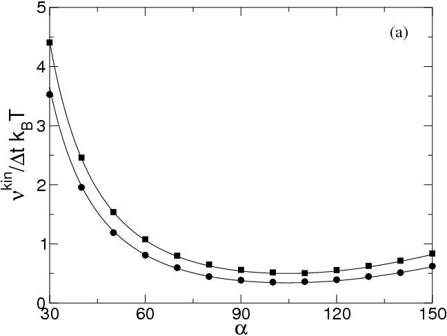
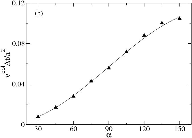
Figure 1: (a) Normalized kinetic contribution to the viscosity, $\nu^{kin}/(\Delta tk_{B}T)$, in three dimensions as a function of the collision angle $\alpha$. Data were obtained by time averaging the Green-Kubo relation over 75,000 iterations using $\lambda/a=2.309$ for $M=5$ ($\blacksquare$) and $M=20$ ($\bullet$). The lines are the theoretical prediction, Eq. (30). Parameters: $L/a=32$, $\Delta t=1$. From Ref. tuzel_03_tcs . (b) Normalized collisional contribution to the viscosity, $\nu^{col}\Delta t/a^{2}$, in three dimensions as a function of the collision angle $\alpha$. The solid line is the theoretical prediction, Eq. (37). Data were obtained by time averaging the Green-Kubo relation over 300,000 iterations. Parameters: $L/a=16$, $\lambda/a=0.1$, $M=3$, and $\Delta t=1$. From Ref. tuzel_thesis .

Collisional contributions: Explicit expressions for the collisional contributions to the viscous transport coefficients can be obtained by considering various choices for ${\bf\hat{k}}$ and $\alpha$ and $\beta$ in Eqs. (4.1), (25) and (4.1.1). Taking ${\bf\hat{k}}$ in the $y$-direction and $\alpha=\beta=1$ yields

$$\nu_{1}^{col}+\nu_{2}^{col}=\frac{1}{\Delta tNk_{B}T}\left.\sum_{t=0}^{\infty}\right.^{\prime}\sum_{i,j}\langle v_{ix}(0)B_{iy}(0)v_{ix}(t)B_{iy}(t)\rangle.$$ (31)

Other choices lead to relations between the collisional contributions to the viscous transport coefficients, namely

$$[1+(d-2)/d]\nu_{1}^{col}+\gamma^{col}+\kappa^{col}=\nu_{1}^{col}+\nu_{2}^{col}.$$ (32)

and

$$[(d-2)/d]\nu_{1}^{col}-\nu_{2}^{col}+\gamma^{col}=0.$$ (33)

These results imply that $\kappa^{col}=0$, and $\gamma^{col}-2\nu_{1}^{col}/d=\nu_{2}^{col}-\nu_{1}^{col}$. It follows that the collision contribution to the macroscopic viscous stress tensor is

$$\hat{\sigma}^{col}_{\alpha\beta}/\rho = \nu_{1}^{col}(\partial_{\beta}v_{\alpha}+\partial_{\alpha}v_{\beta})+\nu_{2}^{col}(\partial_{\beta}v_{\alpha}-\partial_{\alpha}v_{\beta})+(\nu_{2}^{col}-\nu_{1}^{col})\delta_{\alpha\beta}\partial_{\lambda}v_{\lambda}$$ (34)

$$= (\nu_{1}^{col}+\nu_{2}^{col})\partial_{\beta}v_{\alpha}+(\nu_{2}^{col}-\nu_{1}^{col})Q_{\alpha\beta},$$

where $Q_{\alpha\beta}\equiv\delta_{\alpha\beta}\partial_{\lambda}v_{\lambda}-\partial_{\alpha}v_{\beta}$. Since $Q_{\alpha\beta}$ has zero divergence, $\partial_{\beta}Q_{\alpha\beta}=0$, the term containing $Q$ in Eq. (34) will not appear in the linearized hydrodynamic equation for the momentum density, so that

$$\rho\frac{\partial{\bf v}}{\partial t}=-\nabla p+\rho(\nu^{kin}+\nu^{col})\Delta{\bf v}+\frac{d-2}{d}\nu^{kin}\nabla(\nabla\cdot{\bf v}),$$ (35)

where $\nu^{col}=\nu_{1}^{col}+\nu_{2}^{col}$. In writing Eq. (35) we have used the fact that the kinetic contribution to the microscopic stress tensor, $\bar{\sigma}^{kin}$, is symmetric, and $\gamma^{kin}=0$ ihle_03_srd_b . The viscous contribution to the sound attenuation coefficient is $\nu^{col}+2(d-1)\nu^{kin}/d$ instead of the standard result, $2(d-1)\nu/d+\gamma$, for simple isotropic fluids. The collisional contribution to the effective shear viscosity is $\nu^{col}\equiv\nu_{1}^{col}+\nu_{2}^{col}$. It is interesting to note that the kinetic theory approach discussed in Ref. pool_05_ktd is able to show explicitly that $\nu_{1}^{col}=\nu_{2}^{col}$, so that $\nu^{col}=2\nu_{1}^{col}$.

It is straightforward to evaluate the various contributions to the right hand side of (31). In particular, note that since velocity correlation functions are only required at equal times and for a time lag of one time step, molecular chaos can be assumed ihle_04_rgr . Using the relation ihle_05_ect

$$\langle B_{i\alpha}(n\Delta t)B_{j\beta}(m\Delta t)\rangle={a^{2}\over 12}\,\delta_{\alpha\beta}(1+\delta_{ij})\left[2\delta_{n,m}-\delta_{n,m+1}-\delta_{n,m-1}\right]\,,$$ (36)

and averaging over the number of particles in a cell assuming that the number of particles in any cell is Poisson distributed at each time step, with an average number $M$ of particles per cell, one then finds

$$\nu^{col}=\nu_{1}^{col}+\nu_{2}^{col}=\frac{a^{2}}{6d\Delta t}\left(\frac{M-1+e^{-M}}{M}\right)[1-\cos(\alpha)]\;,$$ (37)

for the SRD collision rules in both two and three dimensions. Eq. (37) agrees with the result of Refs. kiku_03_tcm and pool_05_ktd obtained using a completely different non-equilibrium approach in shear flow. Simulation results for the collisional contribution to the viscosity are in excellent agreement with this result (see Fig. 1).

Thermal diffusivity and self-diffusion coefficient: As with the viscosity, there are both kinetic and collisional contributions to the thermal diffusivity, $D_{T}$. A detailed analysis of both contributions is given in Ref. ihle_05_ect , and the results are summarized in Table 1. The self-diffusion coefficient, $D$, of particle $i$ is defined by

$$D=\lim_{t\to\infty}\frac{1}{2dt}\langle[{\bf r}_{i}(t)-{\bf r}_{i}(0)]^{2}\rangle=\frac{\Delta t}{d}\left.\sum_{n=0}^{\infty}\right.^{\prime}\langle{\bf v}_{i}(n\Delta t)\cdot{\bf v}_{i}(0)\rangle,$$ (38)

where the second expressions is the corresponding discrete GK relation. The self-diffusion coefficient is unique in that the collisions do not explicitly contribute to $D$. With the assumption of molecular chaos, the kinetic contributions are easily summed ihle_03_srd_b to obtain the result given in Table 1.

4.1.2 Beyond Molecular Chaos

The kinetic contributions to the transport coefficients presented in Table 1 have all been derived under the assumption of molecular chaos, i.e., that particle velocities are not correlated. Simulation results for the shear viscosity and thermal diffusivity have generally been found to be in good agreement with these results. However, it is known that there are correlation effects for $\lambda/a$ smaller than unity ripo_05_drf ; ihle_06_sdp . They arise from correlated collisions between particles that are in the same collision cell for more than one time step.

For the viscosity and thermal conductivity, these corrections are generally negligible, since they are only significant in the small $\lambda/a$ regime, where the collisional contribution to the transport coefficients dominates. In this regard, it is important to note that there are no correlation corrections to $\nu^{col}$ and $D_{T}^{col}$ ihle_05_ect . For the self-diffusion coefficient—for which there is no collisional contribution—correlation corrections dramatically increase the value of this transport coefficient for $\lambda\ll a$, see Refs. ripo_05_drf ; ihle_06_sdp . These correlation corrections, which arise from particles which collide with the same particles in consecutive time steps, are distinct from the correlations effects which are responsible for the long-time tails. This distinction is important, since long-time tails are also visible at large mean free paths, where these corrections are negligible.

	$d$	Kinetic$~{}~{}(\times k_{B}T\Delta t/2m)$	Collisional$~{}~{}(\times a^{2}/\Delta t)$
$\nu$	2	$\frac{M}{(M-1+e^{-M})\sin^{2}(\alpha)}-1$	$\frac{\left(M-1+e^{-M}\right)}{6dM}[1-\cos(\alpha)]$
	3	$\frac{5M}{(M-1+e^{-M})[2-\cos(\alpha)-\cos(2\alpha)]}-1$
$D_{T}$	2	$\frac{d}{1-\cos(\alpha)}-1+\frac{2d}{M}\left[\frac{7-d}{5}-\frac{1}{4}\,{\csc^{2}(\alpha/2)}\right]$	$\frac{(1-1/M)}{3(d+2)M}[1-\cos(\alpha)]$
	3
$D$	2	$\frac{dM}{(1-\cos(\alpha))(M-1+e^{-M})}-1$	-
	3

Table 1: Theoretical expressions for the kinematic shear viscosity $\nu$, the thermal diffusivity, $D_{T}$, and the self-diffusion coefficient, $D$, in both two ($d=2$) and three ($d=3$) dimensions. $M$ is the average number of particles per cell, $\alpha$ is the collision angle, $k_{B}$ is Boltzmann’s constant, $T$ is the temperature, $\Delta t$ is the time step, $m$ is the particle mass, and $a$ is the cell size. Except for self-diffusion constant, for which there is no collisional contribution, both the kinetic and collisional contributions are listed. The expressions for shear viscosity and self-diffusion coefficient include the effect of fluctuations in the number of particles per cell; however, for brevity, the relations for thermal diffusivity are correct only up to $O(1/M)$ and $O(1/M^{2})$ for the kinetic and collisional contributions, respectively. For the complete expressions, see Refs. ihle_05_ect ; tuzel_03_tcs ; tuzel_thesis .

4.2 Dynamic Structure Factor

Spontaneous thermal fluctuations of the density, $\rho({\bf r},t)$, the momentum density, ${\bf g}({\bf r},t)$, and the energy density, $\epsilon({\bf r},t)$, are dynamically coupled, and an analysis of their dynamic correlations in the limit of small wave numbers and frequencies can be used to measure a fluid’s transport coefficients. In particular, because it is easily measured in dynamic light scattering, x-ray, and neutron scattering experiments, the Fourier transform of the density-density correlation function—the dynamics structure factor—is one of the most widely used vehicles for probing the dynamic and transport properties of liquids berne_00_dls .

A detailed analysis of equilibrium dynamic correlation functions—the dynamic structure factor as well as the vorticity and entropy-density correlation functions—using the SRD algorithm is presented in Ref. tuzel_06_dcs . The results—which are in good agreement with earlier numerical measurements and theoretical predictions—provided further evidence that the analytic expressions or the transport coefficients are accurate and that we have an excellent understanding of the SRD algorithm at the kinetic level.

Here, we briefly summarize the results for the dynamic structure factor. The dynamic structure exhibits three peaks, a central “Rayleigh” peak caused by the thermal diffusion, and two symmetrically placed “Brillouin peaks” caused by sound. The width of the central peak is determined by the thermal diffusivity, $D_{T}$, while that of the two Brillouin peaks is related to the sound attenuation coefficient, $\Gamma$. For the SRD algorithm tuzel_06_dcs ,

$$\Gamma=D_{T}\left(\frac{c_{p}}{c_{v}}-1\right)+2\left(\frac{d-1}{d}\right)\nu^{kin}+\nu^{col}.$$ (39)

Note that in two-dimensions, the sound attenuation coefficient for a SRD fluid has the same functional dependence on $D_{T}$ and $\nu=\nu^{kin}+\nu^{col}$ as an isotropic fluid with an ideal-gas equation of state (for which $\gamma=0$).

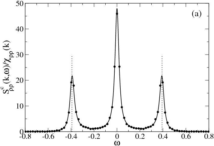
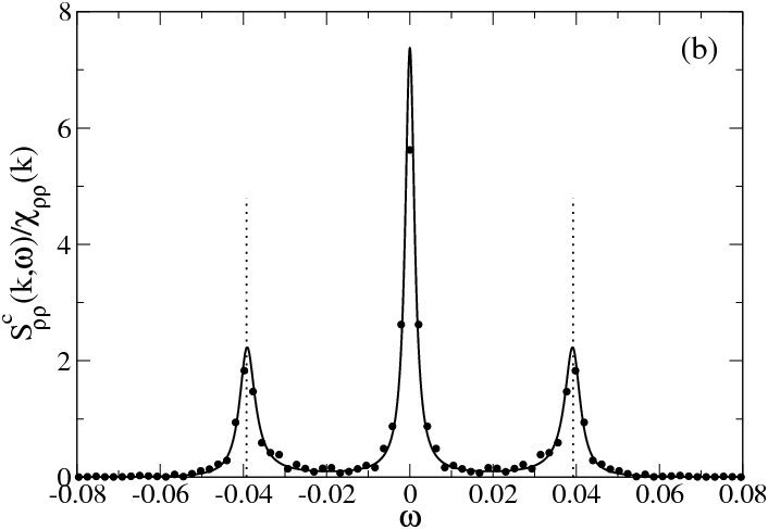
Figure 2: Normalized dynamic structure, $S^{c}_{\rho\rho}(k\omega)/\chi_{\rho\rho}(k)$, for ${\bf k}=2\pi(1,1)/L$ and (a) $\lambda/a=1.0$ with $\alpha=120^{\circ}$, and (b) $\lambda/a=0.1$ with $\alpha=60^{\circ}$. The solid lines are the theoretical prediction for the dynamic structure factor (see Eq. (36) of Ref. tuzel_06_dcs ) using values for the transport coefficients obtained using the expressions in Table 1. The dotted lines show the predicted positions of the Brillouin peaks, $\omega=\pm ck$, with $c=\sqrt{2k_{B}T/m}$. Parameters: $L/a=32$, $M=15$, and $\Delta t=1.0$. From Ref. tuzel_06_dcs .

Simulation results for the structure factor in two-dimensions with $\lambda/a=1.0$ and collision angle $\alpha=120^{\circ}$, and $\lambda/a=0.1$ with collision angle $\alpha=60^{\circ}$ are shown in Figs. 2a and 2b, respectively. The solid lines are the theoretical prediction for the dynamic structure factor (see Eq. (36) of Ref. tuzel_06_dcs ) using $c=\sqrt{2k_{B}T/m}$ and values for the transport coefficients obtained using the expressions in Table 1, assuming that the bulk viscosity $\gamma=0$. As can be seen, the agreement is excellent.

5 Non-Equilibrium Calculations of Transport Coefficients

MPC transport coefficients have also be evaluated by calculating the linear response of the system to imposed gradients. This approach was introduced by Kikuchi et al. kiku_03_tcm for the shear viscosity and then extended and refined in Ref. pool_05_ktd to determine the thermal diffusivity and bulk viscosity. Here, we summarize the derivation of the shear viscosity.

5.1 Shear Viscosity of SRD: Kinetic Contribution

Linear response theory provides an alternative, and complementary, approach for evaluating the shear viscosity. This non-equilibrium approach is related to equilibrium calculations described in the previous section through the fluctuation-dissipation theorem. Both methods yield identical results. For the more complicated analysis of the hydrodynamic equations, the stress tensor, and the longitudinal transport coefficients such as the thermal conductivity, the reader is referred to Ref. pool_05_ktd .

Following Kikuchi et al. kiku_03_tcm , we consider a two-dimensional liquid with an imposed shear $\dot{\gamma}=\partial u_{x}(y)/\partial y$. On average, the velocity profile is given by ${\bf v}=(\dot{\gamma}y,0)$. The dynamic shear viscosity $\eta$ is the proportionality constant between the velocity gradient $\dot{\gamma}$ and the frictional force acting on a plane perpendicular to $y$; i.e.

$$\sigma_{xy}=\eta\dot{\gamma},$$ (40)

where $\sigma_{xy}$ is the off-diagonal element of the viscous stress tensor. During the streaming step, particles will cross this plane only if $|v_{y}\,\Delta t|$ is greater than the distance to the plane. Assuming that the fluid particles are homogeneously distributed, the momentum flux is obtained by integrating over the coordinates and velocities of all particles that cross the plane from above and below during the time step $\Delta t$. The result is kiku_03_tcm

$$\sigma_{xy}=\rho\left({\dot{\gamma}\Delta t\over 2}\,\langle v_{y}^{2}\rangle-\langle v_{x}v_{y}\rangle\right)\,,$$ (41)

where the mass density $\rho=mM/a^{d}$, and the averages are taken over the steady-state distribution $P(v_{x}-\dot{\gamma}y,v_{y})$. It is important to note that this is not the Maxwell-Boltzmann distribution, since we are in a non-equilibrium steady state where the shear has induced correlations between $v_{x}$ and $v_{y}$. As a consequence, $\langle v_{x}v_{y}\rangle$ is nonzero. To determine the behavior of $\langle v_{x}v_{y}\rangle$, the effect of streaming and collisions are calculated separately. During streaming, particles which arrive at $y_{0}$ with positive velocity $v_{y}$ have started from $y_{0}-v_{y}\,\Delta t$; these particles bring a velocity component $v_{x}$ which is smaller than that of particles originally located at $y_{0}$. On the other hand, particles starting out at $y>y_{0}$ with negative $v_{y}$ bring a larger $v_{x}$. The velocity distribution is therefore sheared by the streaming, so that $P^{after}(v_{x},v_{y})=P^{before}(v_{x}+\dot{\gamma}v_{y}\Delta t,v_{y})$. Averaging $v_{x}v_{y}$ over this distribution gives kiku_03_tcm

$$\langle v_{x}v_{y}\rangle^{after}=\langle v_{x}v_{y}\rangle-\dot{\gamma}\Delta t\langle v_{y}^{2}\rangle\,,$$ (42)

where the superscript denotes the quantity after streaming. The streaming step therefore reduces correlations by $-\dot{\gamma}\Delta t\langle v_{y}^{2}\rangle$, making $v_{x}$ and $v_{y}$ increasingly anti-correlated.

The collision step redistributes momentum between particles and tends to reduce correlations. Making the assumption of molecular chaos, i.e., that is that the velocities of different particles are uncorrelated, and averaging over the two possible rotation directions, one finds,

$$\langle v_{x}v_{y}\rangle^{after}=\left[1-{N_{c}-1\over N_{c}}[1-\cos(2\alpha)]\right]\,\langle v_{x}v_{y}\rangle^{before}$$ (43)

The number of particles in a cell, $N_{c}$ is not constant, and density fluctuations have to be included. The probability to find $n$ uncorrelated particles in a given cell is given by the Poisson distribution, $w(n)=\exp(-M)M^{n}/n!$; the probability of a given particle being in a cell together with $n-1$ others is $nw(n)/M$. Taking an average over this distribution gives

$$\langle v_{x}v_{y}\rangle^{after}=f\,\langle v_{x}v_{y}\rangle^{before},$$ (44)

with

$$f=\left[1-\frac{M-1+\exp(-M)}{M}[1-\cos(2\alpha)]\right].$$ (45)

The difference between this result and just replacing $N_{c}$ by $M$ in Eq. (43) is small, and only important for $M\leq 3$. One sees that $\langle v_{x}v_{y}\rangle$ is first modified by streaming and then multiplied by a factor $f$ in the subsequent collision step. In the steady state, it therefore oscillates between two values. Using Eqs. (42), (44), and (45), we obtain the self-consistency condition $(\langle v_{x}v_{y}\rangle-\dot{\gamma}\Delta t\langle v_{y}^{2}\rangle)f=\langle v_{x}v_{y}\rangle$. Solving for $\langle v_{x}v_{y}\rangle$, assuming equipartition of energy, $\langle v_{y}^{2}\rangle=k_{B}T/m$, and substituting into (41), we have

$$\sigma_{xy}={\dot{\gamma}\,M\Delta tk_{B}T\over m}\left({1\over 2}+{f\over 1-f}\right)\,,$$ (46)

Inserting this result into the definition of the viscosity, (40), yields the same expression for the kinetic viscosity in two-dimensional as obtained by the equilibrium Green-Kubo approach discussed in Sec. 4.1.1.

5.2 Shear Viscosity of SRD: Collisional Contribution

The collisional contribution to the shear viscosity is proportional to $a^{2}/\Delta t$; as discussed in Sec. 3.2, it results from the momentum transfer between particles in a cell of size $a$ during the collision step. Consider again a collision cell of linear dimension $a$ with a shear flow $u_{x}(y)=\dot{\gamma}y$. Since the collisions occur in a shifted grid, they cause a transfer of momentum between neighboring cells of the original unshifted reference frame ihle_01_srd ; ihle_03_srd_b . Consider now the momentum transfer due to collisions across the line $y=h$, the coordinate of a cell boundary in the unshifted frame. If we assume a homogeneous distribution of particles in the collision cell, the mean velocities in the upper ($y>h$) and lower partitions are

$${\bf u}_{1}=\frac{1}{M_{1}}\,\sum_{i=1}^{M_{1}}\,{\bf v}_{i}\ \ \ \ {\rm and}\ \ \ \ {\bf u}_{2}=\frac{1}{M_{2}}\,\sum_{i=M_{1}+1}^{M}\,{\bf v}_{i}\,,$$ (47)

respectively, where $M_{1}=M(a-h)/a$ and $M_{2}=Mh/a$. Collisions transfer momentum between the two parts of the cell. The $x$-component of the momentum transfer is

$$\Delta p_{x}(h)\equiv\sum_{i=1}^{M_{1}}\,[v_{ix}^{after}-v_{ix}^{before}]\;\;.$$ (48)

The use of the rotation rule (2) together with an average over the sign of the stochastic rotation angle yields

$$\Delta p_{x}(h)=[\cos(\alpha)-1]M_{1}(u_{1x}-u_{x})\;\;.$$ (49)

Since $M{\bf u}=M_{1}{\bf u}_{1}+M_{2}{\bf u}_{2}$,

$$\Delta p_{x}(h)=[1-\cos(\alpha)]\,M\,(u_{2x}-u_{1x})\,\,\frac{h}{a}\,\left(1-\frac{h}{a}\right)\;\;.$$ (50)

Averaging over the position $h$ of the dividing line, which corresponds to averaging over the random shift, we find

$$\langle\Delta p_{x}\rangle=\frac{1}{a}\int_{0}^{a}\Delta p_{x}(h)dh=\frac{1}{6}[1-\cos(\alpha)]M(u_{2x}-u_{1x}).$$ (51)

Since the dynamic viscosity $\eta$ is defined as the ratio of the tangential stress, $P_{yx}$, to $\partial u_{x}/\partial y$, we have

$$\eta=\frac{\langle\Delta p_{x}\rangle/(a^{2}\Delta t)}{\partial u_{x}/\partial y}=\frac{\langle\Delta p_{x}\rangle/(a^{2}\Delta t)}{(u_{2x}-u_{1x})/(a/2)},$$ (52)

so that the kinematic viscosity, $\nu=\eta/\rho$, in two-dimensions for SRD is

$$\nu^{col}=\frac{a^{2}}{12\Delta t}[1-\cos(\alpha)]$$ (53)

in the limit of small mean free path. Since we have neglected the fluctuations in the particle number, this expression corresponds to the limit $M\rightarrow\infty$. Even though this derivation is somewhat heuristic, it gives a remarkably accurate expression; in particular, it contains the correct dependence on the cell size, $a$, and the time step, $\Delta t$, in the limit of small free path,

$$\nu^{col}=\frac{a^{2}}{\Delta t}f_{col}(d,M,\alpha),$$ (54)

as expected from simple random walk arguments. Kikuchi et al. kiku_03_tcm included particle number fluctuations and obtained identical results for the collisional contribution to the viscosity as was obtained in the Green-Kubo approach (see Table 1).

5.3 Shear Viscosity of MPC-AT

For MPC-AT, the viscosities have been calculated in Ref. nogu_07_pmh using the methods described in Secs. 5.1 and 5.2. The total viscosity of MPC-AT is given by the sum of two terms, the collisional and kinetic contributions. For MPC-AT-a, it was found for both two and three dimensions that nogu_07_pmh

$$\nu^{kin} = {k_{B}T\Delta t\over m}\left({M\over M-1+{\rm e}^{-M}}-{1\over 2}\right)\ \ \ \ \ \ {\rm and}$$

$$\nu^{col} = {a^{2}\over 12\Delta t}\left({M-1+{\rm e}^{-M}\over M}\right).$$ (55)

The exponential terms ${\rm e}^{-M}$ are due to the fluctuation of the particle number per cell and become important for $M\leq 3$. As was the case for SRD, the kinetic viscosity has no anti-symmetric component; the collisional contribution, however, does. Again, as discussed in Sec. 4.1.1 for SRD, one finds $\nu_{1}^{col}=\nu_{2}^{col}=\nu^{col}/2$. This relation is true for all $-a$ versions of MPC discussed in Refs. gg:gomp07f ; nogu_07_pmh ; nogu_08_ang . Simulation results were found to be in good agreement with theory.

For MPC-AT+a it was found for sufficiently large $M$ that gotz_07_ram ; nogu_08_ang

$$\nu^{kin} = {k_{B}T\Delta t\over m}\left({M\over M-(d+2)/4}-{1\over 2}\right),$$

$$\nu^{col} = {a^{2}\over 24\Delta t}\left({M-7/5\over M}\right).$$ (56)

MPC-AT-a and MPC-AT+a both have the same kinetic contribution to the viscosity in two dimensions; however, imposing angular-momentum conservation makes the collisional contribution to the stress tensor symmetric, so that the asymmetric contribution, $\nu_{2}$, discussed in Sec. 4.1.1 vanishes. The resulting collisional contribution to the viscosity is then reduced by a factor close to two.

6 Generalized MPC Algorithms for Dense Liquids and Binary Mixtures

The original SRD algorithm models a single-component fluid with an ideal-gas equation of state. The fluid is therefore very compressible, and the speed of sound, $c_{s}$, is low. In order to have negligible compressibility effects, as in real liquids, the Mach number has to be kept small, which means that there are limits on the flow velocity in the simulation. The SRD algorithm can be modified to model both excluded volume effects, allowing for a more realistic modeling of dense gases and liquids, as well as repulsive hard-core interactions between components in mixtures, which allow for a thermodynamically consistent modeling of phase separating mixtures.

6.1 Non-Ideal Model

As in SRD, the algorithm consists of individual streaming and collision steps. In order to define the collisions, a second grid with sides of length $2a$ is introduced, which (in $d=2$) groups four adjacent cells into one “supercell”. The cell structure is sketched in Fig. 3 (left panel). To initiate a collision, pairs of cells in every supercell are chosen at random. Three different choices are possible: a) horizontal (with $\mbox{\boldmath$\sigma$}_{1}=\hat{x}$), b) vertical ($\mbox{\boldmath$\sigma$}_{2}=\hat{y}$), and c) diagonal collisions (with $\mbox{\boldmath$\sigma$}_{3}=(\hat{x}+\hat{y})/\sqrt{2}$ and $\mbox{\boldmath$\sigma$}_{4}=(\hat{x}-\hat{y})/\sqrt{2}$).

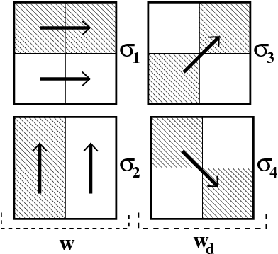
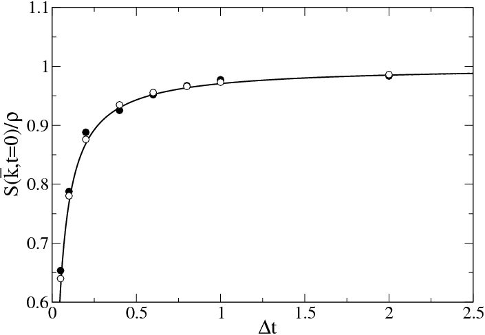
Figure 3: (left panel) Schematic of collision rules. Momentum is exchanged in three ways: a) horizontally along $\mbox{\boldmath$\sigma$}_{1}$, b) vertically along $\mbox{\boldmath$\sigma$}_{2}$, and c) diagonally along $\mbox{\boldmath$\sigma$}_{3}$ and $\mbox{\boldmath$\sigma$}_{4}$. $w$ and $w_{d}$ denote the probabilities of choosing collisions a), b), and c) respectively. (right panel) Static structure factor $S(\bar{k},t=0)$ as a function of $\Delta t$ for $M=3$. The open circles ($\circ$) show results obtained by taking the numerical derivative of the pressure. The bullets ($\bullet$) are data obtained from direct measurements of the density fluctuations. The solid line is the theoretical prediction obtained using the first term in Eq. (59) and Eq. (61). $\bar{k}$ is the smallest wave vector, $\bar{k}=(2\pi/L)(1,0)$. Parameters: $L/a=32$, $A=1/60$, and $k_{B}T=1.0$. From Ref. ihle_06_cpa .

For a mean particle velocity ${\bf u}_{n}=(1/M_{n})\,\sum_{i=1}^{M_{n}}\,{\bf v}_{i}$, of cell $n$, the projection of the difference of the mean velocities of the selected cell pairs on ${\bf\sigma}_{j}$, $\Delta u={\bf\sigma}_{j}\cdot({\bf u}_{1}-{\bf u}_{2})$, is then used to determine the probability of collision. If $\Delta u<0$, no collision will be performed. For positive $\Delta u$, a collision will occur with an acceptance probability, $p_{A}$, which depends on $\Delta u$ and the number of particles in the two cells, $N_{1}$ and $N_{2}$. The choice of $p_{A}$ determines both the equation of state and the values of the transport coefficients. While there is considerable freedom in choosing $p_{A}$, the requirement of thermodynamic consistency imposes certain restrictions ihle_06_cpa ; ihle_06_sdp ; tuzel_06_ctc . One possible choice is

$$p_{A}(M_{1},M_{2},\Delta u)=\Theta(\Delta u)\,\,{\rm tanh}(\Lambda)\ \ \ \ {\rm with}\ \ \ \ \Lambda=A\,\Delta u\,N_{1}N_{2},$$ (57)

where $\Theta$ is the unit step function and $A$ is a parameter which is used to tune the equation of state. The choice $\Lambda\sim N_{1}N_{2}$ leads to a non-ideal contribution to the pressure which is quadratic in the particle density.

The collision rule chosen in Ref. ihle_06_cpa maximizes the momentum transfer parallel to the connecting vector $\mbox{\boldmath$\sigma$}_{j}$ and does not change the transverse momentum. It exchanges the parallel component of the mean velocities of the two cells, which is equivalent to a “reflection” of the relative velocities, $v_{i}^{\|}(t+\Delta t)-u^{\|}=-(v_{i}^{\|}(t)-u^{\|})$, where $u^{\|}$ is the parallel component of the mean velocity of the particles of both cells. This rule conserves momentum and energy in the cell pairs.

Because of $x-y$ symmetry, the probabilities for choosing cell pairs in the $x$- and $y$- directions (with unit vectors $\mbox{\boldmath$\sigma$}_{1}$ and $\mbox{\boldmath$\sigma$}_{2}$ in Fig. 3) are equal, and will be denoted by $w$. The probability for choosing diagonal pairs ($\mbox{\boldmath$\sigma$}_{3}$ and $\mbox{\boldmath$\sigma$}_{4}$ in Fig. 3) is given by $w_{d}=1-2w$. $w$ and $w_{d}$ must be chosen so that the hydrodynamic equations are isotropic and do not depend on the orientation of the underlying grid. An equivalent criterion is to guarantee that the relaxation of the velocity distribution is isotropic. These conditions require $w=1/4$ and $w_{d}=1/2$. This particular choice also ensures that the kinetic part of the viscous stress tensor is isotropic tuze_07_mmf .

6.1.1 Transport Coefficients

The transport coefficients can be determined using the same Green-Kubo formalism as was used for the original SRD algorithm ihle_01_srd ; ihle_04_rgr . Alternatively, the non-equilibrium approach describe in Sec. 5 can be used. Assuming molecular chaos and ignoring fluctuations in the number of particles per cell, the kinetic contribution to the viscosity is found to be

$$\nu^{kin}={k_{B}T\over m}\,\Delta t\left({1\over p_{col}}-{1\over 2}\right)\,\ \ \ {\rm with}\ \ \ p_{col}=A\,\sqrt{k_{B}T\over m\pi}\;M^{3/2},$$ (58)

which is in good agreement with simulation data. $p_{col}$ is essentially the collision rate, and can be obtained by averaging the acceptance probability, Eq. (57). The collisional contribution to the viscosity is $\nu^{col}=p_{col}(a^{2}/3\Delta t)$ ihle_08 . The self-diffusion constant, $D$, is evaluated by summing over the velocity-autocorrelation function (see, e.g. Ref. ihle_01_srd ); which yields $D=\nu_{kin}$.

6.1.2 Equation of State

The collision rules conserve the kinetic energy, so that the internal energy should be the same as that of an ideal gas. Thermodynamic consistency therefore requires that the non-ideal contribution to the pressure is linear in $T$. This is possible if the coefficient $A$ in Eq. (57) is sufficiently small.

The mechanical definition of pressure—the average longitudinal momentum transfer across a fixed interface per unit time and unit surface area—can be used to determine the equation of state. Only the momentum transfer due to collisions needs to be considered, since that coming from streaming constitutes the ideal part of the pressure. Performing this calculation for a fixed interface and averaging over the position of the interface, one finds the non-ideal part of the pressure,

$$P_{n}=\left({1\over 2\sqrt{2}}+{1\over 4}\right){A\,M^{2}\over 2}{k_{B}T\over a\Delta t}+O(A^{3}T^{2}).$$ (59)

$P_{n}$ is quadratic in the particle density, $\rho=M/a^{2}$, as it would be expected from a virial expansion. The prefactor $A$ must be chosen small enough that higher order terms in this expansion are negligible. Prefactors $A$ leading to acceptance rates of about $15\%$ are sufficiently small to guarantee that the pressure is linear in $T$.

The total pressure is the average of the diagonal part of the microscopic stress tensor,

$$P=P_{id}+P_{n}=\frac{1}{\Delta tL_{x}\,L_{y}}\left\langle\sum_{j}\{\Delta tv_{jx}^{2}-\Delta v_{jx}\,z^{s}_{jlx}/2\}\right\rangle.$$ (60)

The first term gives the ideal part of the pressure, $P_{id}$, as discussed in Ref. ihle_01_srd . The average of the second term is the non-ideal part of the pressure, $P_{n}$. ${\bf z}^{s}_{jl}$ is a vector which indexes collision partners. The first subscript denotes the particle number and the second, $l$, is the index of the collision vectors $\mbox{\boldmath$\sigma$}_{l}$ in Fig. 3 (left panel). The components of ${\bf z}^{s}_{jl}$ are either $0$, $1$, or $-1$ ihle_06_sdp . Simulation results for $P_{n}$ obtained using Eq. (60) are in good agreement with the analytical expression, Eq. (59). In addition, measurements of the static structure factor $S(k\to 0,t=0)$ agree with the thermodynamic prediction

$$S(k\to 0,t=0)=\rho k_{B}T\partial\rho/\partial P|_{T}$$ (61)

when result (59) is used [see Fig. 3 (right panel)]. The adiabatic speed of sound obtained from simulations of the dynamic structure factor is also in good agreement with the predictions following from Eq. (59). These results provide strong evidence for the thermodynamic consistency of the model. Consistency checks are particularly important because the non-ideal algorithm does not conserve phase-space volume. This is because the collision probability depends on the difference of collision-cell velocities, so that two different states can be mapped onto the same state by a collision. While the dynamics presumably still obeys detailed—or at least semi-detailed—balance, this is very hard to prove, since it would require knowledge not only of the transition probabilities, but also of the probabilities of the individual equilibrium states. Nonetheless, no inconsistencies due to the absence of time-reversal invariance or a possible violation of detailed balance have been observed.

The structure of $S(k)$ for this model is also very similar to that of a simple dense fluid. In particular, for fixed $M$, both the depth of the minimum at small $k$ and the height of the first peak increase with decreasing $\Delta t$, until there is an order-disorder transition. The four-fold symmetry of the resulting ordered state—in which clusters of particles are concentrated at sites with the periodicity close, but not necessarily equal, to that of the underlying grid—is clearly dictated by the structure of the collision cells. Nevertheless, these ordered structures are similar to the low-temperature phase of particles with a strong repulsion at intermediate distances, but a soft repulsion at short distances. The scaling behavior of both the self-diffusion constant and the pressure persists until the order/disorder transition.

6.2 Phase-Separating Multi-Component Mixtures

In a binary mixture of A and B particles, phase separation can occur when there is an effective repulsion between A-B pairs. In the current model, this is achieved by introducing velocity-dependent multi-particle collisions between A and B particles. There are $N_{A}$ and $N_{B}$ particles of type A and B, respectively. In two dimensions, the system is coarse-grained into $(L/a)^{2}$ cells of a square lattice of linear dimension $L$ and lattice constant $a$. The generalization to three dimensions is straightforward.

Collisions are defined in the same way as in the non-ideal model discussed in the previous section. Now, however, two types of collisions are possible for each pair of cells: particles of type A in the first cell can undergo a collision with particles of type B in the second cell; vice versa, particles of type B in the first cell can undergo a collision with particles of type A in the second cell. There are no A-A or B-B collisions, so that there is an effective repulsion between A-B pairs. The rules and probabilities for these collisions are chosen in the same way as in the non-ideal single-component fluid described in Refs. ihle_06_cpa ; ihle_06_sdp . For example, consider the collision of A particles in the first cell with the B particles in the second. The mean particle velocity of A particles in the first cell is ${\bf u}_{A}=(1/N_{c,A})\,\sum_{i=1}^{N_{c,A}}\,{\bf v}_{i}$, where the sum runs over all A particles, $N_{c,A}$, in the first cell. Similarly, ${\bf u}_{B}=(1/N_{c,B})\,\sum_{i=1}^{N_{c,B}}\,{\bf v}_{i}$ is the mean velocity of B particles in the second cell. The projection of the difference of the mean velocities of the selected cell-pairs on ${\bf\sigma}_{j}$, $\Delta u_{AB}={\bf\sigma}_{j}\cdot({\bf u}_{A}-{\bf u}_{B})$, is then used to determine the probability of collision. If $\Delta u_{AB}<0$, no collision will be performed. For positive $\Delta u_{AB}$, a collision will occur with an acceptance probability

$$p_{A}(N_{c,A},N_{c,B},\Delta u_{AB})=A\,\Delta u_{AB}\,\Theta(\Delta u_{AB})\,N_{c,A}N_{c,B}\,,$$ (62)

where $\Theta$ is the unit step function and $A$ is a parameter which allows us to tune the equation of state; in order to ensure thermodynamic consistency, it must be sufficiently small that that $p_{A}<1$ for essentially all collisions. When a collision occurs, the parallel component of the mean velocities of colliding particles in the two cells, $v_{i}^{\|}(t+\Delta t)-u_{AB}^{\|}=-(v_{i}^{\|}(t)-u_{AB}^{\|})$, is exchanged, where $u_{AB}^{\|}=(N_{c,A}u^{\|}_{A}+N_{c,B}u^{\|}_{B})/(N_{c,A}+N_{c,B})$ is the parallel component of the mean velocity of the colliding particles. The perpendicular component remains unchanged. It is easy to verify that these rules conserve momentum and energy in the cell pairs. The collision of B particles in the first cell with A particles in the second is handled in a similar fashion.

Because there are no A-A and B-B collisions, additional SRD collisions at the cell level are incorporated in order to mix particle momenta. The order of A-B and SRD collision is random, i.e., the SRD collision is performed first with a probability $1/2$. If necessary, the viscosity can be tuned by not performing SRD collisions every time step. The results presented here were obtained using a SRD collision angle of $\alpha=90^{\circ}$.

The transport coefficients can be calculated in the same way as for the one-component non-ideal system. The resulting kinetic contribution to the viscosity is

$$\nu^{kin}=\frac{\Delta tk_{B}T}{2}\left(\frac{1}{A}\sqrt{\frac{2\pi}{k_{B}T}}[M_{A}M_{B}(M_{A}+M_{B})]^{-1/2}-1\right)\,,$$ (63)

where $M_{A}=\langle N_{c,A}\rangle$, $M_{B}=\langle N_{c,B}\rangle$. In deep quenches, the concentration of the minority component is very small, and the non-ideal contribution to the viscosity approaches zero. In this case, the SRD collisions provide the dominant contribution to the viscosity.

6.2.1 Free Energy

An analytic expression for the equation of state of this model can be derived by calculating the momentum transfer across a fixed surface, in much the same way as was done for the non-ideal model in Ref. ihle_06_cpa . Since there are only non-ideal collisions between A-B particles, the resulting contribution to the pressure is

$$P_{n}=\left(w+\frac{w_{d}}{\sqrt{2}}\right)AM_{A}M_{B}\frac{k_{B}T}{a\Delta t}=\Gamma\rho_{A}\rho_{B},$$ (64)

where $\rho_{A}$ and $\rho_{B}$ are the densities of A and B and $\Gamma\equiv(w+w_{d}/\sqrt{2})a^{3}A/\Delta t$. In simulations, the total pressure can be measured by taking the ensemble average of the diagonal components of the microscopic stress tensor. In this way, the pressure can be measured locally, at the cell level. In particular, the pressure in a region consisting of $N_{cell}$ cells is

$$P_{n}=\frac{1}{\Delta ta^{2}N_{cell}}\left\langle\sum_{c=1}^{N_{c}}\sum_{j\in c}[{\Delta tv_{jx}^{2}-\Delta v_{jx}z^{s}_{jlx}/2}]\right\rangle,$$ (65)

where the second sum runs over the particles in cell $c$. The first term in Eq. (65) is the ideal-gas contribution to the pressure; the second comes from the momentum transfer between cells involved in the collision indexed by ${\bf z}^{s}_{jl}$ tuze_07_mmf .

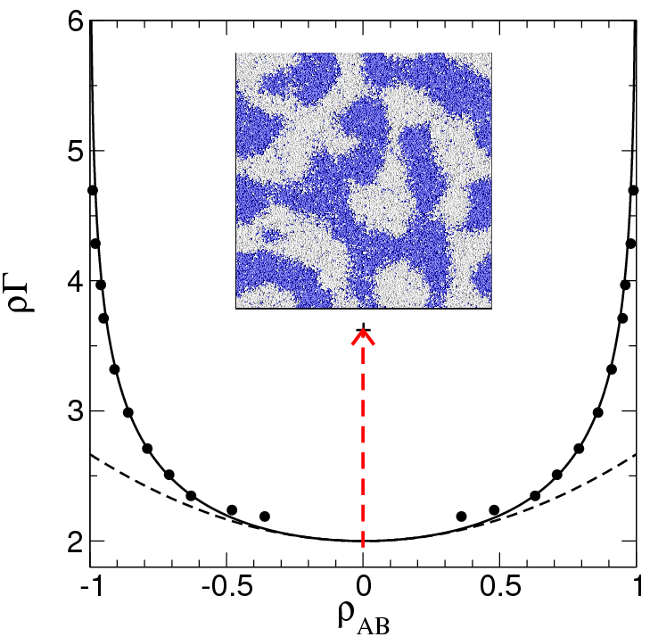
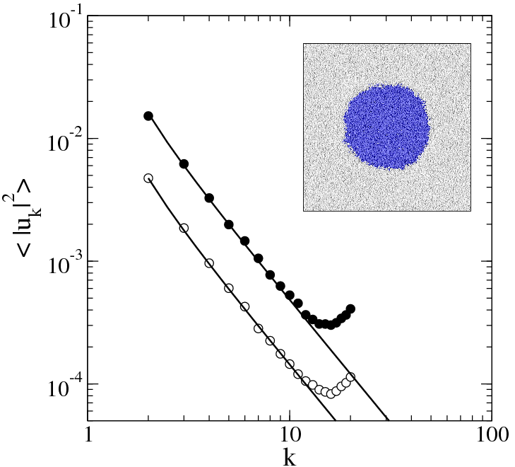
Figure 4: (left panel) Binary phase diagram. There is phase separation for $\rho\Gamma>2$. Simulation results for $\rho_{AB}$ obtained from concentration histograms are shown as bullets. The dashed line is a plot of the leading singular behavior, $\rho_{AB}=\sqrt{3(\rho\Gamma-2)/2}$, of the order parameter at the critical point. The inset shows a configuration 50,000 time steps after a quench along $\rho_{AB}=0$ to $\rho\Gamma=3.62$ (arrow). The dark (blue) and light (white) spheres are A and B particles, respectively. Parameters: $L/a=64$, $M_{A}=M_{B}=5$, $k_{B}T=0.0004$, $\Delta t=1$, and $a=1$. From Ref. tuze_07_mmf . (right panel) Dimensionless radial fluctuations, $\langle|u_{k}^{2}|\rangle$, as a function of the mode number $k$ for $A=0.45$ ($\bullet$) and $A=0.60$ ($\circ$) with $k_{B}T=0.0004$. The average droplet radii are $r_{0}=11.95\,a$ and $r_{0}=15.21\,a$, respectively. The solid lines are fits to Eq. (69). The inset shows a typical droplet configuration for $\rho_{AB}=-0.6$, $\rho\Gamma=3.62$ ($A=0.60$ and $k_{B}T=0.0004$). Parameters: $L/a=64$, $M_{A}=2$, $M_{B}=8$, $\Delta t=1$, and $a=1$. From Ref. tuze_07_mmf .

Expression (64) can be used to determine the entropy density, $s$. The ideal-gas contribution to $s$ has the form callen_60_t

$$s_{ideal}=\rho\,\varphi(T)-k_{B}[\rho_{A}\ln\rho_{A}+\rho_{B}\ln\rho_{B}],$$ (66)

where $\rho=\rho_{A}+\rho_{B}$. Since $\varphi(T)$ is independent of $\rho_{A}$ and $\rho_{B}$, this term does not play a role in the current discussion. The non-ideal contribution to the entropy density, $s_{n}$, can be obtained from Eq. (64) using the thermodynamic relation

$$P_{n}/T=-s_{n}+\rho_{A}\partial s_{n}/\partial\rho_{A}+\rho_{B}\partial s_{n}/\partial\rho_{B}.$$ (67)

The result is $s_{n}=\Gamma\rho_{A}\rho_{B}$, so that the total configurational contribution to the entropy density is

$$s=-k_{B}\left\{\rho_{A}\ln\rho_{A}+\rho_{B}\ln\rho_{B}+\Gamma\rho_{A}\rho_{B}\right\}.$$ (68)

Since there is no configurational contribution to the internal energy in this model, the mean-field phase diagram can be determined by maximizing the entropy at fixed density $\rho$. The resulting demixing phase diagram as a function of $\rho_{AB}=(\rho_{A}-\rho_{B})/\rho$ is given by the solid line in Fig. 4 (left panel). The critical point is located at $\rho_{AB}=0$, $\rho\Gamma^{*}=2$. For $\rho\Gamma<2$, the order parameter $\rho_{AB}=0$; for $\rho\Gamma>2$, there is phase separation into coexisting A- and B-rich phases. As can be seen, the agreement between the mean-field predictions and simulation results is very good except close to the critical point, where the histogram method of determining the coexisting densities is unreliable and critical fluctuations influence the shape of the coexistence curve.

6.2.2 Surface Tension

A typical configuration for $\rho_{AB}=0$, $\rho\Gamma=3.62$ is shown in the inset to Fig. 4 (left panel), and a snapshot of a fluctuating droplet at $\rho_{AB}=-0.6$, $\rho\Gamma=3.62$ is shown in the inset to Fig. 4 (right panel). The amplitude of the capillary wave fluctuations of a droplet is determined by the surface tension, $\sigma$. Using the parameterization $r(\phi)=r_{0}\left[1+\sum_{k=-\infty}^{\infty}u_{k}\exp(ik\phi)\right]$ and choosing $u_{0}$ to fix the area of the droplet, it can be shown that tuzel_thesis

$$\langle|u_{k}|^{2}\rangle=\frac{k_{B}T}{2\pi r_{0}\sigma}\left(\frac{1}{k^{2}-1}\right).$$ (69)

Figure 4 (right panel) contains a plot of $\langle|u_{k}|^{2}\rangle$ as a function of mode number $k$ for $\rho\Gamma=3.62$ and $\rho\Gamma=2.72$. Fits to the data yield $\sigma\simeq 2.9\,k_{B}T$ for $\rho\Gamma=3.62$ and $\sigma\simeq 1.1\,k_{B}T$ for $\rho\Gamma=2.72$. Mechanical equilibrium requires that the pressure difference across the interface of a droplet satisfies the Laplace equation

$$\Delta p=p_{in}-p_{out}=(d-1)\sigma/r_{0}$$ (70)

in $d$ spatial dimensions. Measurements of $\Delta p$ [using Eq. (65)] as a function of the droplet radius for $A=0.60$ at $k_{B}T=0.0005$ yield results in excellent agreement with the Laplace equation for the correct value of the surface tension tuze_07_mmf .

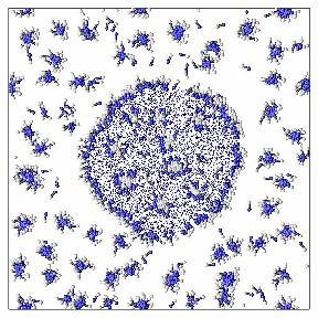
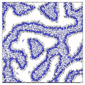
Figure 5: (left panel) Droplet configuration in a mixture with $N_{A}=8192$, $N_{B}=32768$, and $N_{d}=1500$ dimers after $10^{5}$ time steps. The initial configuration is a droplet with a homogeneous distribution of dimers. The dark (blue) and light (white) colored spheres indicate A and B particles, respectively. For clarity, A particles in the bulk are smaller and B particles in the bulk are not shown. Parameters: $L/a=64$, $M_{A}=2$, $M_{B}=8$, $A=1.8$, $k_{B}T=0.0001$, $\Delta t=1$, and $a=1$. (right panel) Typical configuration showing the bicontinuous phase for $N_{A}=N_{B}=20480$ and $N_{d}=3000$. Parameters: $L/a=64$, $M_{A}=5$, $M_{B}=5$, $A=1.8$, $k_{B}T=0.0001$, $\Delta t=1$, and $a=1$. From Ref. tuze_07_mmf .

The model therefore displays the correct thermodynamic behavior and interfacial fluctuations. It can also be extended to model amphiphilic mixtures by introducing dimers consisting of tethered A and B particles. If the A and B components of the dimers participate in the same collisions as the solvent, they behave like amphiphilic molecules in binary oil-water mixtures. The resulting model displays a rich phase behavior as a function of $\rho\Gamma$ and the number of dimers, $N_{d}$. Both the formation of droplets and micelles, as shown in Fig. 5 (left panel), and a bicontinuous phase, as illustrated in Fig. 5 (right panel), have been observed tuze_07_mmf . The coarse-grained nature of the algorithm therefore enables the study of large time scales with a feasible computational effort.

6.2.3 Color Models for Immiscible Fluids

There have been other generalizations of SRD to model binary mixtures by Hashimoto et al. hash_00_irl and Inoue et al. inou_04_msm , in which a color charge, $c_{i}=\pm 1$ is assigned to two different species of particles. The rotation angle $\alpha$ in the SRD rotation step is then chosen such that the color-weighted momentum in a cell, ${\bf m}=\sum_{i=1}^{N_{c}}c_{i}({\bf v}_{i}-{\bf u})$, is rotated to point in the direction of the gradient of the color field $\bar{c}=\sum_{i=1}^{N_{c}}c_{i}$. This rule also leads to phase separation. Several tests of the model have been performed; Laplace’s equation was verified numerically, and simulation studies of spinodal decomposition and the deformation of a falling droplet were performed hash_00_irl . Later applications include a study of the transport of slightly deformed immiscible droplets in a bifurcating channel inou_06_ams . Subsequently, the model was generalized through the addition of dumbbell-shaped surfactants to model micellization sakai_00_fmr and the behavior of ternary amphiphilic mixtures in both two and three dimensions saka_02_rlm ; sakai_02_taf . Note that since the color current after the collision is always parallel to the color gradient, thermal fluctuations of the order parameter are neglected in this approach.

7 Boundary Conditions and Embedded Objects

7.1 Collisional Coupling to Embedded Particles

A very simple procedure for coupling embedded objects such as colloids or polymers to a MPC solvent has been proposed in Ref. male_00_dsp . In this approach, every colloid particle or monomer in the polymer chain is taken to be a point-particle which participates in the SRD collision. If monomer $i$ has mass $m_{m}$ and velocity ${\bf w}_{i}$, the center of mass velocity of the particles in the collision cell is

$${\bf u}=\frac{m\sum_{i=1}^{N_{c}}{\bf v}_{i}+m_{m}\sum_{i=1}^{N_{m}}{\bf w}_{i}}{N_{c}m+N_{m}m_{m}},$$ (71)

where $N_{m}$ is the number of monomers in the collision cell. A stochastic collision of the relative velocities of both the solvent particles and embedded monomers is then performed in the collision step. This results in an exchange of momentum between the solvent and embedded monomers. The same procedure can of course be employed for other MPC algorithms, such as MPC-AT. The new monomer momenta are then used as initial conditions for a molecular-dynamics update of the polymer degrees of freedom during the subsequent streaming time step, $\Delta t$. Alternatively, the momentum exchange, $\Delta p$, can be included as an additional force $\Delta p/\Delta t$ in the molecular-dynamics integration. If there are no other interactions between monomers—as might be the case for embedded colloids—these degrees of freedom stream freely during this time interval.

When using this approach, the average mass of solvent particles per cell, $mN_{c}$, should be of the order of the monomer or colloid mass $m_{m}$ (assuming one embedded particle per cell) ripo_05_drf . This corresponds to a neutrally buoyant object which responds quickly to the fluid flow but is not kicked around too violently. It is also important to note that the average number of monomers per cell, $\langle N_{m}\rangle$, should be smaller than unity in order to properly resolve hydrodynamic interactions between the monomers. On the other hand, the average bond length in a semi-flexible polymer or rod-like colloid should also not be much larger than the cell size $a$, in order to capture the anisotropic friction of rod-like molecules due to hydrodynamic interactions gg:gomp08b (which leads to a twice as large perpendicular than parallel friction coefficient for long stiff rods doi:86 ), and to avoid an unnecessarily large ratio of the number of solvent to solute particles. For a polymer, the average bond length should therefore be of the order of $a$.

In order to use SRD to model suspended colloids with a radius of order $1\mu$m in water, this approach would require approximately 60 solvent particles per cell in order to match the Peclet number hecht_05_scc . This is much larger than the optimum number (see discussion in Sec. 2.2.1), and the relaxation to the Boltzmann distribution is very slow. Because of its simplicity and efficiency, this monomer-solvent coupling has been used in many polymer falc_03_dst ; ripo_04_lhc ; wink:04 ; muss:05 ; webs_05_mtp and colloid simulations falc_04_ihm ; hecht_05_scc ; ripo_05_drf ; hecht_07_sta .

7.2 Thermal Boundaries

In order to accurately resolve the local flow field around a colloid, more accurate methods have been proposed which exclude fluid-particles from the interior of the colloid and mimic slip male_00_smd ; lee_04_fdb or no-slip inou_02_dsm boundary conditions. The latter procedure is similar to what is known in molecular dynamics as a “thermal wall” boundary condition: fluid particles which hit the colloid particle are given a new, random velocity drawn from the following probability distributions for the normal velocity component, $v_{N}$, and the tangential component, $v_{T}$,

$$p_{N}(v_{N}) = (mv_{N}/k_{B}T)\,\exp\left(-{mv_{N}^{2}/2k_{B}T}\right)\,,\ \ {\rm with}\ \ v_{N}>0\,,$$

$$p_{T}(v_{T}) = \sqrt{m/2\pi k_{B}T}\,\exp\left(-{mv_{T}^{2}/2k_{B}T}\right)\,.$$ (72)

These probability distributions are constructed so that the probability distribution for particles near the wall remains Maxwellian. The probability distribution, $p_{T}$, for the tangential components of the velocity is Maxwellian, and both positive and negative values are permitted. The normal component must be positive, since after scattering at the surface, the particle must move away from the wall. The form of $p_{N}$ is a reflection of the fact that more particles with large $|v_{N}|$ hit the wall per unit time than with small $|v_{N}|$ inou_02_dsm .

This procedure models a no-slip boundary condition at the surface of the colloid, and also thermostats the fluid at the boundaries. For many non-equilibrium flow conditions, this may not be sufficient, and it may also be necessary to thermostat the bulk fluid also (compare Sec. 2.3). It should also be noted that Eqs. (72) will be a good approximation only if the radius of the embedded objects is much larger than the mean free path $\lambda$. For smaller particles, corrections are needed.

If a particle hits the surface at time $t_{0}$ in the interval between $n\Delta t$ and $(n+1)\Delta t$, the correct way to proceed would be to give the particle its new velocity and then have it stream the remaining time $(n+1)\Delta t-t_{0}$. However, such detailed resolution is not necessary. It has been found hecht_05_scc that good results are also obtained using the following simple stochastic procedure. If a particle is found to have penetrated the colloid during the streaming step, one simply moves it to the boundary and then stream a distance ${\bf v}_{new}\,\Delta t\,\epsilon$, where $\epsilon$ is a uniformly distributed random number in the interval [0,1].

Another subtlety is worth mentioning. If two colloid particles are very close, it can happen that a solvent particle could hit the second colloid after scattering off the first, all in the interval $\Delta t$. Naively, one might be tempted to simply forbid this from happening or ignore it. However, this would lead to a strong depletion-like attractive force between the colloids hecht_05_scc . This effect can be greatly reduced by allowing multiple collisions in which one solvent particle is repeatedly scattered off the two colloids. In every collision, momentum is transferred to one of the colloids, which pushes the colloids further apart. In practice, even allowing for up to ten multiple collisions cannot completely cancel the depletion interaction—one needs an additional repulsive force to eliminate this unphysical attraction. The same effect can occur when a colloid particle is near a wall.

Careful tests of this thermal coupling have been performed by Padding et al. padd_05_stick ; padd_06_hib , who were able to reproduce the correct rotational diffusion of a colloid. It should be noted that because the coupling between the solvent particles and the surface occurs only through the movement of the fluid particles, the coupling is quite weak for small mean free paths.

7.3 Coupling using Additional Forces

Another procedure for coupling an embedded object to the solvent has been pursued by Kapral et al. male_00_smd ; lee_01_csd ; kapr_08_mpc . They introduce a central repulsive force between the solvent particles and the colloid. This force has to be quite strong in order to prohibit a large number of solvent particles from penetrating the colloid. When implementing this procedure, a small time step $\delta t$ is therefore required in order to resolve these forces correctly, and a large number of molecular dynamics time steps are needed during the SRD streaming step. In its original form, central forces were used, so that only slip boundary conditions could be modeled. In principle, non-central forces could be used to impose no-slip conditions.

This approach is quite natural and very easy to implement; it does, however, require the use of small time steps and therefore may not be the optimal procedure for many applications.

7.4 “Ghost” or “Wall” Particles

One of the first approaches employed to impose a non-slip boundary condition at an external wall or at a moving object in a MPC solvent was to use “ghost” or “wall” particles lamu_01_mcd ; lamu_02_nsf . In other mesoscale methods such as Lattice-Boltzmann, no-slip conditions are modeled using the bounce-back rule: the velocity of particle is inverted from ${\bf v}$ to $-{\bf v}$ when it intersects a wall. For planar walls which coincide with the boundaries of the collision cells, the same procedure can be used in MPC. However, the walls will generally not coincide with, or even be parallel to, the cell walls. Furthermore, for small mean free paths, where a shift of the cell lattice is required to guarantee Galilean invariance, partially occupied boundary cells are unavoidable, even in the simplest flow geometries.

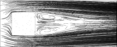
Figure 6: Velocity field of a fluid near a square cylinder in a Poiseuille flow at Reynolds number $Re=v_{max}L/\nu=30$. The channel width is eight times larger than the cylinder size $L$. A pair of stationary vortices are seen behind the obstacle, as expected for $Re\leq 60$. From Ref. lamu_02_nsf .

The simple bounce-back rule fails to guarantee no-slip boundary conditions in the case of partially filled cells. The following generalization of the bounce-back rule has therefore been suggested. For all cells that are cut by walls, fill the “wall” part of the cell with a sufficient number of virtual particles in order to make the total number of particles equal to $M$, the average number of particles per cell. The velocities of the wall particles are drawn from a Maxwell-Boltzmann distribution with zero mean velocity and the same temperature as the fluid. The collision step is then carried out using the mean velocity of all particles in the cell. Note that since Gaussian random numbers are used, and the sum of Gaussian random numbers is also Gaussian-distributed, the velocities of the individual wall particles need not to be determined explicitly. Instead, the average velocity ${\bf u}$ can be written as ${\bf u}=(\sum_{i=1}^{n}{\bf v}_{i}+{\bf a})/M$, where ${\bf a}$ is vector whose components are Gaussian random numbers with zero mean and variance $(M-n)k_{B}T$. Results for Poiseuille flow obtained using this procedure, both with and without cell shifting, were found to be in excellent agreement with the correct parabolic profile lamu_01_mcd . Similarly, numerical results for the recirculation length, the drag coefficient, and the Strouhal number for flows around a circular and square cylinder in two dimensions were shown to be in good agreement with experimental results and computational fluid dynamics data for a range of Reynolds numbers between $Re=10$ and $Re=130$ (see Fig. 6) lamu_01_mcd ; lamu_02_nsf .

8 Importance of Angular-Momentum Conservation: Couette Flow

As an example of a situation in which it is important to use an algorithm which conserves angular momentum, consider a drop of a highly viscous fluid inside a lower-viscosity fluid in circular Couette flow. In order to avoid the complications of phase-separating two-component fluids, the high viscosity fluid is confined to a radius $r<R_{1}$ by an impenetrable boundary with reflecting boundary conditions (i.e., the momentum parallel to the boundary is conserved in collisions). No-slip boundary conditions between the inner and outer fluids are guaranteed because collision cells reach across the boundary. When a torque is applied to the outer circular wall (with no-slip, bounce-back boundary conditions) of radius $R_{2}>R_{1}$, a solid-body rotation of both fluids is expected. The results of simulations with both MPC-AT$-a$ and MPC-AT$+a$ are shown in Fig. 7. While MPC-AT$+a$ reproduces the expected behavior, MPC-AT$-a$ produces different angular velocities in the two fluids, with a low (high) angular velocity in the fluid of high (low) viscosity gotz_07_ram .

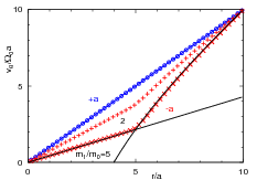
Figure 7: Azimuthal velocity of binary fluids in a rotating cylinder with $\Omega_{0}=0.01(k_{B}T/m_{0}a^{2})^{1/2}$. The viscous fluids with particle mass $m_{1}$ and $m_{0}$ are located at $r<R_{1}$ and $R_{1}<r<R_{2}$, respectively, with $R_{1}=5a$ and $R_{2}=10a$. Symbols represent the simulation results of MPC-AT$-a$ with $m_{1}/m_{0}=2$ ($+$) or $m_{1}/m_{0}=5$ ($\times$), and MPC-AT$+a$ for $m_{1}/m_{0}=5$ ($\circ$). Solid lines represent the analytical results for MPC-AT$-a$ at $m_{1}/m_{0}=5$. Error bars are smaller than the size of the symbols. From Ref. gotz_07_ram .

The origin of this behavior is that the viscous stress tensor in general has symmetric and antisymmetric contributions (see Sec. 4.1.1),

$$\sigma_{\alpha\beta}=\lambda(\partial_{\gamma}v_{\gamma})\delta_{\alpha\beta}+\bar{\eta}\left(\partial_{\beta}v_{\alpha}+\partial_{\alpha}v_{\beta}\right)+\check{\eta}\left(\partial_{\beta}v_{\alpha}-\partial_{\alpha}v_{\beta}\right),$$ (73)

where $\lambda$ is the second viscosity coefficient and $\bar{\eta}\equiv\rho\nu_{1}$ and $\check{\eta}\equiv\rho\nu_{2}$ are the symmetric and anti-symmetric components of the viscosity, respectively. The last term in Eq. (73) is linear in the vorticity $\nabla\times{\bf v}$, and does not conserve angular momentum. This term therefore vanishes (i.e., $\check{\eta}=0$) when angular momentum is conserved.

The anti-symmetric part of the stress tensor implies an additional torque, which becomes relevant when the boundary condition is given by forces. In cylindrical coordinates ($r,\theta,z$), the azimuthal stress is given by gotz_07_ram

$$\sigma_{r\theta}=(\bar{\eta}+\check{\eta})\frac{r\partial(v_{\theta}/r)}{\partial r}+2\check{\eta}\frac{v_{\theta}}{r}.$$ (74)

The first term is the stress of the angular-momentum-conserving fluid, which depends on the derivative of the angular velocity $\Omega=v_{\theta}/r$. The second term is an additional stress caused by the lack of angular momentum conservation; it is proportional to $\Omega$.

In the case of the phase-separated fluids in circular Couette flow, this implies that if both fluids rotate at the same angular velocity, the inner and outer stresses do not coincide. Thus, the angular velocity of the inner fluid $\Omega_{1}$ is smaller than the outer one, with $v_{\theta}(r)=\Omega_{1}r$ for $r<R_{1}$ and

$$v_{\theta}(r)=Ar+B/r,{\rm\ \ with\ \ }A=\frac{\Omega_{2}R_{2}^{2}-\Omega_{1}R_{1}^{2}}{R_{2}^{2}-R_{1}^{2}},\ \ B=\frac{(\Omega_{1}-\Omega_{2})R_{1}^{2}R_{2}^{2}}{R_{2}^{2}-R_{1}^{2}}$$ (75)

for $R_{1}<r<R_{2}$. $\Omega_{1}$ is then obtained from the stress balance at $r=R_{1}$, i.e., $2\check{\eta}_{1}\Omega_{1}=(8/3)\eta_{2}(\Omega_{0}-\Omega_{1})+2\check{\eta}_{2}\Omega_{1}$. This calculation reproduces the numerical results very well, see Fig. 7. Thus, it is essential to employ an $+a$ version of MPC in simulations of multi-phase flows of binary fluids with different viscosities.

There are other situations in which the lack angular momentum conservation can cause significant deviations. In Ref. gotz_07_ram , a star polymer with small monomer spacing was placed in the middle of a rotating Couette cell. As in the previous case, it was observed that the polymer fluid rotated with a smaller angular velocity than the outer fluid. When the angular momentum conservation was switched on, everything rotated at the same angular velocity, as expected.

9 MPC without Hydrodynamics

The importance of hydrodynamic interactions (HI) in complex fluids is generally accepted. A standard procedure for determining the influence of HI is to investigate the same system with and without HI. In order to compare results, however, the two simulations must differ as little as possible—apart from the inclusion of HI. A well-known example of this approach is Stokesian dynamics simulations (SD), where the original Brownian dynamics (BD) method can be extended by including hydrodynamic interactions in the mobility matrix by employing the Oseen tensor doi:86 ; dhon96 .

A method for switching off HI in MPC has been proposed in Refs. kiku_02_pcp ; kiku_03_tcm . The basic idea is to randomly interchange velocities of all solvent particles after each collision step, so that momentum (and energy) are not conserved locally. Hydrodynamic correlations are therefore destroyed, while leaving friction coefficients and fluid self-diffusion coefficients largely unaffected. Since this approach requires the same numerical effort as the original MPC algorithm, a more efficient method has been suggested recently in Ref. ripo_07_hss . If the velocities of the solvent particles are not correlated, it is no longer necessary to follow their trajectories. In a random solvent, the solvent-solute interaction in the collision step can thus be replaced by the interaction with a heat bath. This strategy is related to that proposed in Ref. lamu_01_mcd to model no-slip boundary conditions of solvent particles at a planar wall, compare Sec. 7.4. Since the positions of the solvent particles within a cell are not required in the collision step, no explicit particles have to be considered. Instead, each monomer is coupled with an effective solvent momentum ${\bf P}$ which is directly chosen from a Maxwell-Boltzmann distribution of variance $mMk_{B}T$ and a mean given by the average momentum of the fluid field—which is zero at rest, or $(mM\dot{\gamma}r^{i}_{y},0,0)$ in the case of an imposed shear flow. The total center-of-mass velocity, which is used in the collision step, is then given by ripo_07_hss

$${\bf v}_{cm,i}=\frac{m_{m}{\bf v}_{i}+{\bf P}}{mM+m_{m}},$$ (76)

where $m_{m}$ is the mass of the solute particle. The solute trajectory is then determined using MD, and the interaction with the solvent is performed every collision time $\Delta t$.

The random MPC solvent therefore has similar properties to the MPC solvent, except that there are no HI. The relevant parameters in both methods are the average number of particles per cell, $M$, the rotation angle $\alpha$, and the collision time $\Delta t$ which can be chosen to be the same. For small values of the density ($M<5$), fluctuation effects have been noticed kiku_03_tcm and could also be included in the random MPC solvent by a Poisson-distributed density. The velocity autocorrelation functions ripo_05_drf of a random MPC solvent show a simple exponentially decay, which implies some differences in the solvent diffusion coefficients. Other transport coefficients such as the viscosity depend on HI only weakly tuzel_06_dcs and consequently are expected to be essentially identical in both solvents.

10 Applications to Colloid and Polymer Dynamics

The relevance of hydrodynamic interactions for the dynamics of complex fluids—such as dilute or semidilute polymer solutions, colloid suspensions, and microemulsions—is well known doi:86 ; dhon96 . From the simulation point of view, however, these systems are difficult to study because of the large gap in length- and time-scales between solute and solvent dynamics. One possibility for investigating complex fluids is the straightforward application of molecular dynamics simulations (MD), in which the fluid is course-grained and represented by Lennard-Jones particles. Such simulations provide valuable insight into polymer dynamics pier:91 ; duen:91 ; pier:92 ; duen:93 ; aust:99 . Similarly, mesoscale algorithms such as Lattice-Boltzmann and dissipative particle dynamics have been widely used for modeling of colloidal and polymeric systems boek97 ; ahlr:98 ; ahlr:01 ; spen:00 ; lowe:04 .

Solute molecules, e.g., polymers, are typically composed of a large number of individual particles, whose interactions are described by a force-field. As discussed in Sec. 7, the particle-based character of the MPC solvent allows for an easy and controlled coupling between the solvent and solute particles. Hybrid simulations combining MPC and molecular dynamics simulations are therefore easy to implement. Results of such hybrid simulations are discussed in the following.

10.1 Colloids

Many applications in chemical engineering, geology, and biology involve systems of particles immersed in a liquid or gas flow. Examples include sedimentation processes, liquid-solid fluidized beds, and flocculation in suspensions.

Long-ranged solvent-mediated hydrodynamic interactions have a profound effect on the non-equilibrium properties of colloidal suspensions, and the many-body hydrodynamic backflow effect makes it difficult to answer even relatively simple questions such what happens when a collection of particles sediments through a viscous fluid. Batchelor batch_72_sed calculated the lowest-order volume fraction correction to the average sedimentation velocity, $v_{s}=v_{s}^{0}(1-6.55\,\phi)$, of hard spheres of hydrodynamic radius $R_{H}$ where $v_{s}^{0}$ is the sedimentation velocity of a single sphere. Due to the complicated interplay between short-ranged contact forces and long-ranged HI, it is hard to extend this result to the high volume fraction suspensions of interest for ceramics and soil mechanics. An additional complication is that the Brownian motion of solute particles in water cannot be neglected if they are smaller than $1\mu m$ in diameter.

The dimensionless Peclet number $Pe=v_{s}^{0}R_{H}/D$, where $D$ is the self-diffusion coefficient of the suspended particles, measures the relative strength of HI and thermal motion. Most studies of sedimentation have focused on the limit of infinite Peclet number, where Brownian forces are negligible. For example, Ladd ladd_97_lba employed a Lattice-Boltzmann method (LB), and Hoefler and Schwarzer hoef_00_nss used a marker-and-cell Navier-Stokes solver to simulate such non-Brownian suspensions. The main difficulty with such algorithms is the solid-fluid coupling which can be very tricky: in LB simulations, special “boundary nodes” were inserted on the colloid surface, while in Ref. hoef_00_nss , the coupling was mediated by inertia-less markers which are connected to the colloid by stiff springs and swim in the fluid, effectively dragging the colloid, but also exerting a force on the fluid. Several methods for coupling embedded particles to an MPC solvent were discussed in Sec. 7.

Using the force-based solvent-colloid coupling described in Sec. 7.3, Padding and Louis padd_04_hbf investigated the importance of HI during sedimentation at small Peclet numbers. Surprisingly, they found that the sedimentation velocity does not change if the Peclet number is varied between 0.1 and 15 for a range of volume fractions. For small volume fractions, the numerical results agree with the Batchelor law; for intermediate $\phi$ they are consistent with the semi-empirical Richardson-Zaki law, $v_{s}=v_{s}^{0}(1-\phi)^{n}$, $n=6.55$. Even better agreement was found with theoretical predictions by Hayakawa and Ichiki haya_95_sph ; haya_97_shs , who took higher order HI into account. Purely hydrodynamic arguments are therefore still valid in an average sense at low $Pe$, i.e., for strong Brownian motion and relatively weak HI. This also means that pure Brownian simulations without HI, which lead to $v_{s}=v_{s}^{0}(1-\phi)$, strongly underestimate the effect of backflow.

On the other hand, it is known that the velocity autocorrelation function of a colloidal particle embedded in a fluctuating liquid at equilibrium exhibits a hydrodynamic long-time tail, $\langle v(t)v(0)\rangle\sim t^{-d/2}$, where $d$ is the spatial dimension ernst_70_atb . These tails have been measured earlier for point-like SRD particles in two ihle_01_srd ; ihle_03_srd_b and three ripo_05_drf spatial dimensions, and found to be in quantitative agreement with analytic predictions, with no adjustable parameters. It is therefore not surprising that good agreement was also obtained for embedded colloids padd_04_hbf . MPC therefore correctly describes two of the most important effects in colloidal suspensions, thermal fluctuations and hydrodynamic interactions.

In a series of papers, Hecht et al. hecht_05_scc ; hecht_06_she ; hecht_07_sta used hybrid SRD-molecular dynamics simulations to investigate a technologically important colloidal system—$Al_{2}O_{3}$-particles of diameter $0.5\mu m$ (which is often used in ceramics) suspended in water—with additional colloid-colloid interactions. These colloids usually carry a charge which, by forming an electric double layer with ions in water, results in a screened electrostatic repulsion. The interaction can be approximated by the Derjaguin-Landau-Verwey-Overbeek (DLVO) theory DLVO_1 ; DLVO_2 . The resulting potential contains a repulsive Debye-Hückel contributions, $V_{EL}\sim{\rm exp}(-\kappa[r-d])/r$, where $d$ is the particle diameter, $\kappa$ is the inverse screening length, and $r$ is the distance of the particle centers. The second part of the DLVO-potential is a short-range van der Waals attraction,

$$V_{vdW}=-{A_{H}\over 12}\left[{d^{2}\over r^{2}-d^{2}}+{d^{2}\over r^{2}}+2{\rm ln}\left({r^{2}-d^{2}\over r^{2}}\right)\right],$$ (77)

which turns out to be important at the high volume fractions ($\phi>20\%$) and high salt concentrations of interest. $A_{H}$ is the Hamaker constant which involves the polarizability of the particles and the solvent. DLVO theory makes the assumption of linear polarizability and is valid only at larger distances. It therefore does not include the so-called primary potential minimum at particle contact, which is observed experimentally and is about $30k_{B}T$ deep. Because of this potential minimum, colloids which come in contact rarely become free again. In order to ensure numerical stability for reasonable values of the time step, this minimum was modeled by an additional parabolic potential with depth of order $6k_{B}T$. The particle Reynolds number of the real system is very small, of order $10^{-6}$ to $10^{-7}$. Since it would be too time-consuming to model this Reynolds number, the simulations were performed at $Re\approx 0.02$, which still ensures that the contribution of momentum convection is negligible compared to that of momentum diffusion. However, due to the remaining inertial effects and the non-zero time step, it was still possible that particles partially overlapped in the simulation. This overlap was penalized by an additional potential, frequently used in simulations of granular matter, given by a Hertz-law,

$$V_{Hertz}\sim(d-r)^{5/2}\;\;\;\;{\rm if\;}r<d\,.$$ (78)

SRD correctly describes long-range HI, but it can only resolve hydrodynamic interactions on scales larger than both the mean free path $\lambda$ and the cell size $a$. In a typical simulation with about 1000 colloid particles, a relatively small colloid diameter of about four lattice units was chosen for computational efficiency. This means that HI are not fully resolved at interparticle distances comparable to the colloid diameter, and lubrication forces have to be inserted by hand. Only the most divergent mode, the so-called squeezing mode, was used, $F_{lub}\sim v_{rel}/r_{rel}$, where $r_{rel}$ and $v_{rel}$ are the relative distance and velocity of two colloids, respectively. This system of interacting $Al_{2}O_{3}$-particles was simulated in order to study the dependence of the suspension’s viscosity and structure on shear rate, pH, ionic strength and volume fraction. The resulting stability diagram of the suspension as a function of ionic strength and pH value is shown in Fig. 8 (plotted at zero shear) hecht_07_sta . The pH controls the surface charge density which, in turn, affects the electrostatic interactions between the colloids. Increasing the ionic strength, experimentally achieved by “adding salt”, decreases the screening length $1/\kappa$, so that the attractive forces become more important; the particles start forming clusters. Three different states are observed: (i) a clustered regime, where particles aggregate when van der Waals attractions dominate, (ii) a suspended regime where particles are distributed homogeneously and can move freely—corresponding to a stable suspension favored when electrostatic repulsion prevents clustering but is not strong enough to induce order. At very strong Coulomb repulsion the repulsive regime (iii) occurs, where the mobility of the particles is restricted, and particles arrange in local order which maximizes nearest neighbor distances.

The location of the phase boundaries in Fig. 8 depends on the shear rate. In the clustered phase, shear leads to a breakup of clusters, and for the shear rate $\dot{\gamma}=1000\,s^{-1}$, there are many small clusters which behave like single particles. In the regime where the particles are slightly clustered, or suspended, shear thinning is observed. Shear thinning is more pronounced in the slightly clustered state, because shear tends to reduce cluster size. Reasonable agreement with experiments was achieved, and discrepancies were attributed to polydispersity and the manner in which lubrication forces were approximated, as well as uncertainties how the pH and ionic strength enter the model force parameters.

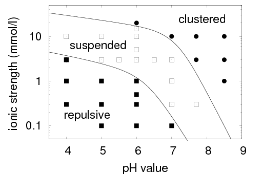
Figure 8: Phase diagram of a colloidal suspension (plotted at zero shear and volume fraction $\phi=35\%$) in the ionic-strength-pH plane depicting three regions: a clustered region, a suspended regime, and a repulsive structure. From Ref. hecht_07_sta .

In the simulations of Hecht et al. hecht_05_scc , the simple collisional coupling procedure described in Sec. 7.1 was used. This means that the colloids were treated as point particles, and solvent particles could flow right through them. Hydrodynamic interactions were therefore only resolved in an average sense, which is acceptable for studies of the general properties of an ensemble of many colloids. The heat from viscous heating was removed using the stochastic thermostat described in Sec. 2.3.

Various methods for modeling no-slip boundary conditions at colloid surfaces—such as the thermal wall coupling described in Sec. 7.2—were systematically investigated in Ref. padd_05_stick . No-slip boundary conditions are important, since colloids are typically not completely spherical or smooth, and the solvent molecules also transfer angular momentum to the colloid. Using the SRD algorithm without angular momentum conservation, it was found that the rotational friction coefficient was larger than predicted by Enskog-theory when the ghost-particle coupling was used padding_private . On the other hand, in a detailed study of the translational and rotational velocity autocorrelation function of a sphere coupled to the solvent by the thermal-wall boundary condition, quantitative agreement with Enskog theory was observed at short times, and with mode-coupling theory at long times. However, it was also noticed that for small particles, the Enskog and hydrodynamic contributions to the friction coefficients were not clearly separated. Specifically, mapping the system to a density matched colloid in water, it appeared that the Enskog and the hydrodynamic contributions are equal at a particle radius of $6\,nm$ for translation and $35.4\,nm$ for rotation; even for a particle radius of $100\,nm$, the Enskog contribution to the friction is still of order $30\%$ and cannot be ignored.

In order to clarify the detailed character of the hydrodynamic interactions between colloids in SRD, Lee and Kapral lee_05_tfm numerically evaluated the fixed-particle friction tensor for two nano-spheres embedded in an SRD solvent. They found that for intercolloidal spacings less than $1.2\,d$, where $d$ is the colloid diameter, the measured friction coefficients start to deviate from the expected theoretical curve. The reader is referred to the review by Kapral kapr_08_mpc for more details.

10.2 Polymer Dynamics

The dynamical behavior of macromolecules in solution is strongly affected or even dominated by hydrodynamic interactions kirk:48 ; erpe:58 ; doi:86 . From a theoretical point of view, scaling relations predicted by the Zimm model for, e.g., the dependencies of dynamical quantities on the length of the polymer are, in general, accepted and confirmed petr:06 . Recent advances in experimental single-molecule techniques provide insight into the dynamics of individual polymers, and raise the need for a quantitative theoretical description in order to determine molecular parameters such as diffusion coefficients and relaxation times. Mesoscale hydrodynamic simulations can be used to verify the validity of theoretical models. Even more, such simulations are especially valuable when analytical methods fail, as for more complicated molecules such as polymer brushes, stars, ultrasoft colloids, or semidilute solutions, where hydrodynamic interactions are screened to a certain degree. Here, mesoscale simulations still provide a full characterization of the polymer dynamics.

We will focus on the dynamics of polymer chains in dilute solution. In order to compare simulation results with theory—in particular the Zimm approach zimm:56 ; doi:86 —and scaling predictions, we address the dynamics of Gaussian as well as self-avoiding polymers.

10.2.1 Simulation Method and Model

Polymer molecules are composed of a large number of equal repeat units called monomers. To account for the generic features of polymers, such as their conformational freedom, no detailed modeling of the basic units is necessary. A coarse-grained description often suffices, where several monomers are comprised in an effective particle. Adopting such an approach, a polymer chain is introduced into the MPC solvent by adding $N_{m}$ point particles, each of mass $m_{m}$, which are connected linearly by bonds. Two different models are considered, a Gaussian polymer and a polymer with excluded-volume (EV) interactions. Correspondingly, the following potentials are applied:
(i) Gaussian chain: The monomers, with the positions ${\vec{r}}_{i}$ ($i=1,\ldots,N_{m}$), are connected by the harmonic potential

$$U_{G}=\frac{3k_{B}T}{2b^{2}}\sum_{i=1}^{N_{m}-1}\left({\vec{r}}_{i+1}-{\vec{r}}_{i}\right)^{2},$$ (79)

with zero mean bond length, and $b$ the root-mean-square bond length. Here, the various monomers freely penetrated each other. This simplification allows for an analytical treatment of the chain dynamics as in the Zimm model zimm:56 ; doi:86 .
(ii) Excluded-volume chain: The monomers are connected by the harmonic potential

$$U_{B}=\frac{\kappa}{2}\sum_{i=1}^{N_{m}-1}\left(|{\vec{r}}_{i+1}-{\vec{r}}_{i}|-b\right)^{2},$$ (80)

with mean bond length $b$. The force constant $\kappa$ is chosen such that the fluctuations of the bond lengths are on the order of a percent of the mean bond length. In addition, non-bonded monomers interact via the repulsive, truncated Lennard-Jones potential

$$U_{LJ}=\left\{\begin{array}[]{cc}4\epsilon\left[\left(\frac{\displaystyle\sigma}{\displaystyle r}\right)^{12}-\left(\frac{\displaystyle\sigma}{\displaystyle r}\right)^{6}\right]+\epsilon,&r<2^{1/6}\sigma\\ 0,&\mbox{otherwise}\end{array}.\right.$$ (83)

The excluded volume leads to swelling of the polymer structure compared to a Gaussian chain, which is difficult to fully account for in analytical calculations muss:05 .

The dynamics of the chain monomers is determined by Newtons’ equations of motion between the collisions with the solvent. These equations are integrated using the velocity Verlet algorithm with the time step $\Delta t_{p}$. The latter is typically smaller than the collision time $\Delta t$. The monomer-solvent interaction is taken into account by inclusion of the monomer of mass $m_{m}=\rho m$ in the collision step male_00_dsp ; muss:05 , compare Sec. 7.1. Alternatively, a Lennard-Jones potential can be used to account for the monomer-MPC particle interaction, where a MPC particle is of zero interaction range male_00_smd ; lee:06 .

We scale length and time according to $\hat{x}=x/a$ and $\hat{t}=t\sqrt{k_{B}T/ma^{2}}$, which corresponds to the choice $k_{B}T=1$, $m=1$, and $a=1$. The mean free path of a fluid particle $\Delta t\sqrt{k_{B}T/m}$ is then given by $\lambda=\Delta\hat{t}$. In addition, we set $b=a$, $\sigma=a$, and $\epsilon/k_{B}T=1$.

The equilibrium properties of a polymer are not affected by hydrodynamic interactions. Indeed, the results for various equilibrium quantities—such as the radius of gyration—of MPC simulation are in excellent agreement with the results of molecular dynamics of Monte Carlo simulations without explicit solvent muss:05 .

Simulations of Gaussian chains, i.e., polymers with the bond potential (79), can be compared with analytical calculations based on the Zimm approach zimm:56 ; doi:86 . Note, however, that the simulations are not performed in the Zimm model. The Zimm approach relies on the preaveraging approximation of hydrodynamic interactions, whereas the simulations take into account the configurational dependence of the hydrodynamic interactions, and therefore hydrodynamic fluctuations. Hence, the comparison can serve as a test of the validity of the approximations employed in the Zimm approach.

The Zimm model rests upon the Langevin equation for over-damped motion of the monomers, i.e., it applies for times larger than the Brownian time scale $\tau_{B}\gg m_{m}/\zeta$, where $\zeta$ is Stokes’ friction coefficient dhon96 . On such time scales, velocity correlation functions have decayed to zero and the monomer momenta are in equilibrium with the solvent. Moreover, hydrodynamic interactions between the various parts of the polymer are assumed to propagate instantaneously. This is not the case in our simulations. First of all, the monomer inertia term is taken into account, which implies non-zero velocity autocorrelation functions. Secondly, the hydrodynamic interactions build up gradually. The center-of-mass velocity autocorrelation function displayed in Fig. 9 reflects these aspects. The correlation function exhibits a long-time tail, which decays as $\left\langle{\vec{v}}_{cm}(t){\vec{v}}_{cm}(0)\right\rangle\sim t^{-3/2}$ on larger time scales. The algebraic decay is associated with a coupling between the motion of the polymer and the hydrodynamic modes of the fluid ernst_70_atb ; ernst_71_atbc ; hansen_86_tsl . A scaling of time with the diffusion coefficient $D$ shows that the correlation function is a universal function of $Dt$. This is in agreement with results of DPD simulations of dilute polymer systems lowe:04 .

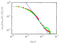
Figure 9: Center-of-mass velocity autocorrelation functions for Gaussian polymers of length $N_{m}=20$, $N_{m}=40$, and $\lambda=0.1$ as a function of $Dt$. The solid line is proportional to $(Dt)^{-3/2}$. From Ref. muss:05 .

The polymer center-of-mass diffusion coefficient follows either via the Green-Kubo relation from the velocity autocorrelation function or by the Einstein relation from the center-of-mass mean square displacement. According to the Kirkwood formula kirk:48 ; erpe:58 ; liu:03

$$D^{(K)}=\frac{D_{0}}{N_{m}}+\frac{k_{B}T}{6\pi\eta}\frac{1}{R_{H}},$$ (84)

where the hydrodynamic radius $R_{H}$ is defined as

$$\frac{1}{R_{H}}=\frac{1}{N_{m}^{2}}\left\langle\sum_{i=1}^{N_{m}}\sum_{j=1}^{N_{m}}{{}^{\prime}}\frac{1}{|{\vec{r}}_{i}-{\vec{r}}_{j}|}\right\rangle$$ (85)

and the prime indicates that the term with $j=i$ has to be left out in the summation. The diffusion coefficient is composed of the local friction contribution $D_{0}/N_{m}$, where $D_{0}$ is the diffusion coefficient of a single monomer in the same solvent, and the hydrodynamic contribution.

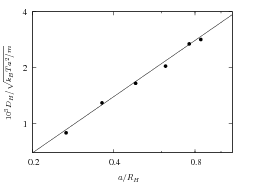
Figure 10: Dependence of the hydrodynamic part of the diffusion coefficient, $D_{H}=D-D_{0}/N_{m}$, on the hydrodynamic radius for Gaussian chains of lengths $N_{m}=5$, $10$, $20$, $40$, $80$, and $160$ (right to left). The mean free path is $\lambda=0.1$. From Ref. muss:05 .

Simulation results for the hydrodynamic contribution, $D_{H}=D-D_{0}/N_{m}$, to the diffusion coefficient are plotted in Fig. 10 as a function of the hydrodynamic radius (85). In the limit $N_{m}\gg 1$, the diffusion coefficient $D$ is dominated by the hydrodynamic contribution $D_{H}$, since $D_{H}\sim N_{m}^{-1/2}$. For shorter chains, $D_{0}/N_{m}$ cannot be neglected, and therefore has to be subtracted in order to extract the scaling behavior of $D_{H}$. The hydrodynamic part of the diffusion coefficient $D_{H}$ exhibits the dependence predicted by the Kirkwood formula and the Zimm theory, i.e., $D_{H}\sim 1/R_{H}$. The finite-size corrections to $D$ show a dependence $D=D_{\infty}-{\rm const}./L$ on the size $L$ of a periodic system, in agreement with previous studies male_00_dsp ; duen:99 ; spen:00 . Simulations for various system sizes for polymers of lengths $N_{m}=10$, $20$, and $40$ allow an extrapolation to infinite system size, which yields $D_{0}/\sqrt{k_{B}Ta^{2}/m}\approx 1.7\times 10^{-2}$, in good agreement with the diffusion coefficient of a monomer in the same solvent. The values of $D_{\infty}$ are about $30\%$ larger than the finite-system-size values presented in Fig. 10. Similarly the diffusion coefficient for a polymer chain with excluded volume interactions displays the dependence $D_{H}\sim 1/R_{H}$ muss:05 .

The Kirkwood formula neglects hydrodynamic fluctuations and is thus identical with the preaveraging result of the Zimm approach. When only the hydrodynamic part is considered, the Zimm model yields the diffusion coefficient

$$D_{Z}=0.192\frac{k_{B}T}{b\eta\sqrt{N_{m}}}.$$ (86)

MPC simulations for polymers of length $N_{m}=40$ yield $D_{Z}/\sqrt{k_{B}Ta^{2}/m}=0.003$. This value agrees with the numerical value for an infinite system, $D_{H}/\sqrt{k_{B}Ta^{2}/m}=0.0027$, within $10\%$. The MPC simulations yield a diffusion coefficient smaller than $D^{(K)}$, in agreement with previous studies presented in Refs. doi:86 ; fixm:83 ; liu:03 . Note that the experimental values are also smaller by about $15\%$ than those predicted by the Zimm approach doi:86 ; schm:81 ; stoc:84 .

To further characterize the internal dynamics of the molecular chain, a mode analysis in terms of the eigenfunctions of the discrete Rouse model rous:53 ; doi:86 has been performed. The mode amplitudes ${\vec{\chi}}_{p}$ are calculated according to

$${\vec{\chi}}_{p}=\sqrt{\frac{2}{N_{m}}}\sum_{i=1}^{N_{m}}{\vec{r}}_{i}\cos\left[\frac{p\pi}{N_{m}}\left(i-\frac{1}{2}\right)\right],\ p=1\ldots N_{m}.$$ (87)

Due to hydrodynamic interactions, Rouse modes are no longer eigenfunctions of the chain molecule. However, within the Zimm theory, they are reasonable approximations and the autocorrelation functions of the mode amplitudes decay exponentially, i.e.,

$$\left\langle{\vec{\chi}}_{p}(t){\vec{\chi}}_{p}(0)\right\rangle=\left\langle{\vec{\chi}}_{p}^{2}\right\rangle\exp\left(-t/\tau_{p}\right).$$ (88)

For the Rouse model, the relaxation times $\tau_{p}$ depend on chain length and mode number according to $\tau_{p}\sim 1/\sin^{2}\left(p\pi/2N_{m}\right)$, whereas for the Zimm model the dependence

$$\tau_{p}\sim(p/N_{m})^{1/2}/\sin^{2}\left(p\pi/2N_{m}\right)$$ (89)

is obtained. The extra contribution $\sqrt{p/N_{m}}$ follows from the eigenfunction representation of the preaveraged hydrodynamic tensor, under the assumption that its off-diagonal elements do not significantly contribute to the relaxation behavior.

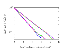
Figure 11: Correlation functions of the Rouse-mode amplitudes for the modes $p=1-4$ of Gaussian polymers. The chain lengths are $N_{m}=20$ (right) and $N_{m}=40$ (left). From Ref. muss:05 .

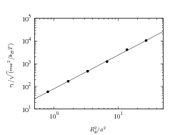
Figure 12: Dependence of the longest relaxation time $\tau_{1}$ on the radius of gyration for Gaussian chains of the lengths given in Fig. 10. From Ref. muss:05 .

In Fig. 11, the autocorrelation functions for the mode amplitudes are shown for the mean free path $\lambda=0.1$. Within the accuracy of the simulations, the correlation functions decay exponentially and exhibit the scaling behavior predicted by the Zimm model. Hence, for the small mean free path, hydrodynamic interactions are taken into account correctly. This is no longer true for the large mean free path, $\lambda=2$. In this case, a scaling behavior between that predicted by the Rouse and Zimm models is observed. This implies that hydrodynamic interactions are present, but are not fully developed or are small compared to the local friction of the monomers. We obtain pure Rouse behavior for a system without solvent by simply rotating the velocities of the individual monomers muss:05 .

The dependence of the longest relaxation time on the radius of gyration is displayed in Fig. 12 for $\lambda=0.1$. The scaling behavior $\tau_{1}\sim R^{3}_{g}$ is in very good agreement with the predictions of the Zimm theory. We even find almost quantitative agreement; the relaxation time of the $p=1$ mode of our simulations is approximately $30$ % larger than the Zimm value doi:86 .

The scaling behavior of equilibrium properties of single polymers with excluded-volume interactions has been studied extensively doi:86 ; dege:79 ; decl:90 ; cepe:81 ; krem:88 . It has been found that even very short chains already follow the scaling behavior expected for much longer chains. In particular, the radius of gyration increases like $R_{G}\sim N_{m}^{\nu}$ with the number of monomers, and the static structure factor $S({\vec{q}})$ exhibits a scaling regime for $2\pi/R_{G}\ll q\ll 2\pi/\sigma$, with a $q^{-1/\nu}$ decay as a function of the scattering vector $q$ and the exponent $\nu\approx 0.6$. For the interaction potentials (80), (83) with the parameters $b=\sigma=a$, $\epsilon/k_{B}T=1$, the exponent $\nu\approx 0.62$ is obtained from the chain-length dependence of the radius of gyration, the mean square end-to-end distance, as well as the $q-$dependence of the static structure factor muss:05 .

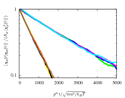
Figure 13: Correlation functions of the Rouse-mode amplitudes for various modes as a function of the scaled time $tp^{\alpha}$ for polymers with excluded volume interactions. The chain lengths are $N_{m}=20$ (left) and $N_{m}=40$ (right). The calculated correlations where fitted by $A_{p}\exp(-t/\tau_{p})$ and have been divided by $A_{p}$. The scaling exponents of the mode numbers are $\alpha=1.93$ ($N_{m}=20$) and $\alpha=1.85$ ($N_{m}=40$), respectively. From Ref. muss:05 .

An analysis of the intramolecular dynamics in terms of the Rouse modes yields non-exponentially decaying autocorrelation functions of the mode amplitudes. At very short times, a fast decay is found, which turns into a slower exponential decay which is well fitted by $A_{p}\exp(-t/\tau_{p})$, see Fig. 13. Within the accuracy of these calculations, the correlation functions exhibit universal behavior. Zimm theory predicts the dependence $\tau_{p}\sim p^{-3\nu}$ for the relaxation times on the mode number for polymers with excluded-volume interactions doi:86 . With $\nu=0.62$, the exponent $\alpha$ for the polymer of length $N_{m}=40$ is found to be in excellent agreement with the theoretical prediction. The exponent for the polymers with $N_{m}=20$ is slightly larger.

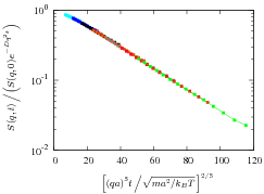
Figure 14: Normalized dynamic structure factor $S({\bf q},t)/(S({\bf q},0)\exp\left(-Dq^{2}t\right))$ of polymers with excluded volume interactions for $N_{m}=40$ and various $q$-values in the range $0.7<qa<2$ as a function of $q^{2}t^{2/3}$. From Ref. muss:05 .

Zimm theory predicts that the dynamic structure factor, which is defined by

$$S({\vec{q}},t)=\frac{1}{N_{m}}\sum_{i=1}^{N_{m}}\sum_{j=1}^{N_{m}}\left\langle\exp\left(i{\vec{q}}[{\vec{r}}_{i}(t)-{\vec{r}}_{j}(0)]\right)\right\rangle,$$ (90)

scales as doi:86

$$S({\vec{q}},t)=S({\vec{q}},0)f(q^{\alpha}t)$$ (91)

with $\alpha=3$ for $qR_{G}\gg 1$, independent of the solvent conditions ($\Theta$ or good solvent). To extract the scaling relation for the intramolecular dynamics, which corresponds to the prediction (91), we resort to the following considerations. As is well known, the dynamic structure factor for a Gaussian distribution of the differences ${\vec{r}}_{i}(t)-{\vec{r}}_{j}(0)$ and a linear equation of motion is given by doi:86 ; wink:97

$$S({\vec{q}},t) = S({\vec{q}},0)e^{-Dq^{2}t}\frac{1}{N_{m}}\sum_{i=1}^{N_{m}}\sum_{j=1}^{N_{m}}\exp\left(-q^{2}\left\langle({\vec{r}}^{\prime}_{i}(t)-{\vec{r}}^{\prime}_{j}(0))^{2}\right\rangle/6\right),$$ (92)

where $Dq^{2}t$ accounts for the center-of-mass dynamics and ${\vec{r}}^{\prime}_{i}$ denotes the position of monomer $i$ in the center-of-mass reference frame. Therefore, in order to obtain the dynamics in the center-of-mass reference frame, we plot $S({\vec{q}},t)/(S({\vec{q}},0)\exp\left(-Dq^{2}t\right))$. The simulation results for the polymer of length $N_{m}=40$, shown in Fig. 14, confirm the predicted scaling behavior. Thus, MPC-MD hybrid simulations are very well suited to study the dynamics of even short polymers in dilute solution.

As mentioned above, the structure of a polymer depends on the nature of the solvent. In good solvent excluded volume interactions lead to expanded conformations and under bad solvent conditions the polymer forms a dense coil. In a number of simulations the influence of hydrodynamic interactions on the transition from an extended to a collapsed state has been studied, when the solvent quality is abruptly changed. Both, molecular dynamics simulations with an explicit solvent chan:01 as well as MPC simulations yeo02 ; yeo05b ; lee:06 yield a significant different dynamics in the presence of hydrodynamic interactions. Specifically, the collapse is faster, with a much weaker dependence of the characteristic time on polymer length yeo05b ; lee:06 , and the folding path is altered.

Similarly, a strong influence of hydrodynamic interactions has been found on the polymer translocation dynamics through a small hole in a wall ali:05 or in polymer packing in a virus capsid ali:04 ; ali:06 . Cooperative backflow effects lead to a rather sharp distribution of translocation times with a peak at relatively short times. The fluid flow field, which is created as a monomer moves through the hole, guides following monomers to move in the same direction.

10.3 Polymers in Flow Fields

Simulations of a MPC fluid confined between surfaces and exposed to a constant external force yield the expected parabolic velocity profile for appropriate boundary conditions lamu_01_mcd ; alla_02_mss ; wata:07 . The ability of MPC to account for the flow behavior of mesoscale objects, such as polymers, under non-equilibrium conditions has been demonstrate for a number of systems. Rod-like colloids in shear flow exhibit flow induced alignment wink:04 . The various diagonal components of the radius of gyration tensor exhibit a qualitative and quantitative different behavior. Due to the orientation, the component in the flow direction increases with increasing Peclet number larger than united and saturates at large shear rates because of finite size effects. The transverse components decrease with shear rate, where the component in the gradient direction is reduced to a greater extent. The rod rotational velocity in the shear plane shows two distinct regimes. For Peclet numbers much smaller than unity, the rotational velocity increases linearly with the shear rate, because the system is isotropic. At Peclet numbers much larger than unity, the shear induced anisotropies lead to a slower increase of the rotational velocity with the shear rate wink:04 .

The simulations of a tethered polymer in a Poiseuille flow webs_05_mtp yield a series of morphological transitions from sphere to deformed sphere to trumpet to stem and flower to rod, similar to theoretically predicted structures broch:93 ; broch:94 ; broch:95 . The crossovers between the various regimes occur at flow rates close to the theoretical estimates for a similar system. Moreover, the simulations in Ref. webs_05_mtp show that backflow effects lead to an effective increase in viscosity, which is attributed to the fluctuations of the free polymer end rather than its shape.

The conformational, structural, and transport properties of free flexible polymers in microchannel flow have been studied in Refs. wata:07 ; cann:07 by hybrid MPC-molecular dynamics simulations. These simulations confirm the cross streamline migration of the molecules as previously observed in Refs. agar:94 ; jend:04 ; usta:06 ; khar:06 ; stei:06 ; usta:07 . In addition, various other polymer properties are addressed in Ref. cann:07 .

All these hybrid simulations confirm that MPC is an excellent method to study the non-equilibrium behavior of polymers in flow fields. In the next section, we will provide a more detailed example for a more complicated object, namely an ultrasoft colloid in shear flow.

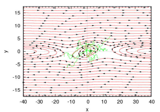
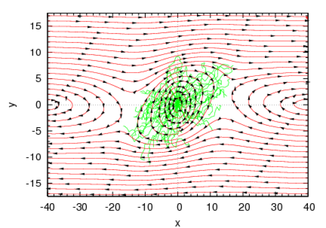
Figure 15: Fluid flow lines in the flow-gradient plane of the star polymer’s center of mass reference frame for $f=10$ (top) and $f=50$ (bottom) arms, both with $L_{f}=20$ monomers per arm and an applied shear field with ${\rm Wi}=\dot{\gamma}\tau=22$. From Ref. ripo_07_hss .

10.4 Ultra-soft Colloids in Shear Flow

Star polymers present a special macromolecular architecture, in which several linear polymers of identical length are linked together by one of their ends at a common center. This structure is particularly interesting because it allows for an almost continuous change of properties from that of a flexible linear polymer to a spherical colloidal particle with very soft interactions. Star polymers are therefore also often called ultrasoft colloids. The properties of star polymers in and close to equilibrium have been studied intensively, both theoretically gres:87 ; liko:01 and experimentally vlas:01 . A star polymer is a ultrasoft colloid, where the core extension is very small compared to the length of an arm. By anchoring polymers on the surface of a hard colloid, the softness can continuously be changed from ultrasoft to hard by increasing the ratio between the core and shell radius at the expense of the thickness of the soft polymer corona. Moreover, star polymers have certain features in common with vesicles and droplets. Although their shell can be softer than that of the other objects, the dense packing of the monomers will lead to a cooperative dynamical behavior resembling that of vesicles or droplets ripo:06 .

Vesicles and droplets encompass fluid which is not exchanged with the surrounding. In contrast, for star-like molecules fluid is free to penetrate into the molecule and internal fluid is exchanged with the surrounding in the course of time. This intimate coupling of the star-polymer dynamics and the fluid flow leads to a strong modification of the flow behavior at and next to the ultrasoft colloid particular in non-equilibrium systems.

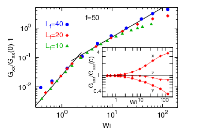
Figure 16: Normalized component $G_{xx}$ of the average gyration tensor as a function of the Weissenberg number ${\rm Wi}$, for star polymers of $f=50$ arms and the arm lengths $L_{f}=10$, $20$, and $40$ monomers. Power-law behaviors with quadratic and linear dependencies on $\rm Wi$ are indicated by lines. The inset shows all three diagonal components of the gyration tensor (for $L_{f}=20$). From Ref. ripo:06 .

In the following, we will discuss a few aspects in the behavior of star polymers in shear flow as a function of arm number $f$, arm length $L_{f}$, and shear rate $\dot{\gamma}$. The polymer model is the same as described in Sec. 10.2.1, where the chain connectivity is determined by the bond potential (80) and the excluded-volume interaction is described by the Lennard-Jones potential (83). A star polymer of functionality $f$ is modeled as $f$ linear polymer chains of $L_{f}$ monomers each, with one of their ends linked to a central particle. Linear polymer molecules are a special case of star polymers with functionality $f=2$. Lees-Edwards boundary conditions alle:87 are employed in order to impose a linear velocity profile $(v_{x},v_{y},v_{z})=(\dot{\gamma}r_{y},0,0)$ in the fluid in the absence of a polymer. For small shear rates, the conformations of star polymers remain essentially unchanged compared to the equilibrium state. Only when the shear rate exceeds a characteristic value, a structural anisotropy as well as an alignment is induced by the flow (cf. Fig. 15). The shear rate dependent quantities are typically presented in terms of the Weissenberg number $\rm Wi=\dot{\gamma}\tau$ rather than the shear rate itself, where $\tau$ is the longest characteristic relaxation time of the considered system. For the star polymers, the best data collapse for stars of various arm lengths is found when the relaxation time $\tau=\eta b^{3}L^{2}_{f}/k_{B}T$ is used ripo:06 . Remarkably, there is essentially no dependence on the functionality. Within the range of investigated star sizes, this relaxation time has to be considered as consistent with the prediction for the blob model of Ref. gres:89 , where $\tau\sim L^{1.8}_{f}f^{0.1}$ for the Flory exponent $\nu=0.6$.

In Fig. 15, typical star conformations are shown which indicate the alignment and induced anisotropy in the flow. Moreover, the figure reveals the intimate coupling of the polymer dynamics and the emerging fluid flow field. In the region, where the fluid coexists with the star polymer, the externally imposed flow field is strongly screened and the fluid velocity is no longer aligned with the shear flow direction, but rotates around the polymer center of mass. The fluid stream lines are calculated by integration of the coarse-grained fluid velocity field. Outside the region covered by the star polymer, the fluid adapts to the central rotation by generating two counter-rotating vortices, and correspondingly two stagnation points of vanishing fluid velocity ripo_07_hss .

The fluid flow in the vicinity of the star polymer is distinctively different from that of a sphere but resembles the flow around an ellipsoid miku:04 . In contrast to the latter, the fluid penetrates into the area covered by the star polymer. While the fluid in the core of the star rotates together with the polymer, the fluid in the corona follows the external flow to a certain extent.

A convenient quantity to characterize the structural properties and alignment of polymers in flow is the average gyration tensor, which is defined as

$$G_{\alpha\beta}({\dot{\gamma}})=\frac{1}{N_{m}}\sum_{i=1}^{N_{m}}\langle r^{\prime}_{i,\alpha}r^{\prime}_{i,\beta}\rangle\ ,$$ (93)

where $N_{m}=fL_{f}+1$ is the total number of monomers, $r^{\prime}_{i,\alpha}$ is the position of monomer $i$ relative to the polymer center of mass, and $\alpha\in\{x,y,z\}$. The average gyration tensor is directly accessible in scattering experiments. Its diagonal components $G_{\alpha\alpha}(\dot{\gamma})$ are the squared radii of gyration of the star polymer along the axes of the reference frame. In the absence of flow, scaling considerations predict gres:87 $G_{xx}(0)=G_{yy}(0)=G_{zz}(0)=R_{g}^{2}(0)/3\sim L_{f}^{2\nu}f^{1-\nu}$.

The diagonal components $G_{\alpha\alpha}$ of the average gyration tensor are shown in Fig. 16 as a function of the Weissenberg number for various functionalities and arm lengths. We find that the extension of a star increases with increasing shear rate in the shear direction ($x$), decreases in the gradient direction ($y$), and is almost independent of $\rm Wi$ in the vorticity direction ($z$). The deviation from spherical symmetry exhibits a ${\rm Wi}^{2}$ power-law dependence for small shear rates for all functionalities. A similar behavior has been found for rod-like colloids wink:04 (due to the increasing alignment with the flow direction) and for linear polymers doi:86 . However, for stars of not too small functionality, a new scaling regime appears, where the deformation seems to scales linearly with the Weissenberg number. For large shear rates, finite-size effects appear due to the finite monomer number. These effects emerge when the arms are nearly stretched, and therefore occur at higher Weissenberg numbers for larger arm lengths.

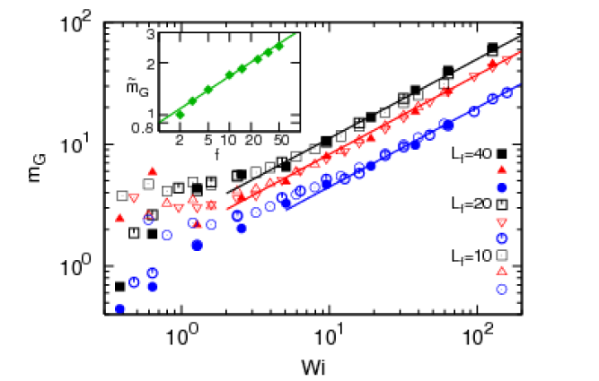
Figure 17: Orientational resistance $m_{G}$ as a function of the Weissenberg number $\rm Wi$ for star polymers with functionalities $f=2$ (circles), $f=15$ (triangles), and $f=50$ (squares), and different arm lengths indicated in the figure. Lines correspond to the power law $m_{G}={\tilde{m}}_{G}(f){\rm Wi}^{0.65}$. The inset shows that the amplitude also follows a power-law behavior with $\tilde{m}_{G}(f)\sim f^{0.27}$. From Ref. ripo:06 .

The average flow alignment of a (star) polymer can be characterized by the orientation angle $\chi_{G}$, which is the angle between the eigenvector of the gyration tensor with the largest eigenvalue and the flow direction. It follows straightforwardly aust:99 from the simulation data via

$$\tan(2\chi_{G})=2G_{xy}/(G_{xx}-G_{yy})\equiv m_{G}/{\rm Wi},$$ (94)

where the right-hand-side of the equation defines the orientation resistance parameter $m_{G}$ link:93 . It has been shown for several systems including rod-like colloids and linear polymers without self-avoidance doi:86 that close to equilibrium $G_{xy}\sim{\dot{\gamma}}$ and $(G_{xx}-G_{yy})\sim{\dot{\gamma}}^{2}$, so that $m_{G}$ is independent of $\rm Wi$. Our results for the orientation resistance are presented in Fig. 17 for various functionalities $f$ and arm lengths $L_{f}$. Data for different $L_{f}$ collapse onto universal curves, which approach a plateau for small shear rates, as expected. For larger shear rates, ${\rm Wi}\gg 1$, a power-law behavior ripo:06

$$m_{G}({\rm Wi})\sim f^{\alpha}\ {\rm Wi}^{\mu},$$ (95)

is obtained with respect to the Weissenberg number and the functionality, where $\alpha=0.27\pm 0.02$ and $\mu=0.65\pm 0.05$. For self-avoiding linear polymers, a somewhat smaller exponent $\mu=0.54\pm 0.03$ was obtained in Refs. aust:99 ; teix:05 , whereas theoretical calculations predict $\sim{\rm Wi}^{2/3}$ in the limit of large Weissenberg numbers wink:06 .

The data for the average orientation and deformation of a star polymer described so far seem to indicate that the properties vary smoothly and monotonically from linear polymers to star polymers of high functionality. However, this picture changes when the dynamical behavior is considered. It is well known by now that linear polymers show a tumbling motion in flow, with alternating collapsed and stretched configurations during each cycle dege:74 ; ledu:99 ; smit:99 ; teix:05 . For large Weissenberg numbers, this leads to very large fluctuations of the largest intramolecular distance of a linear polymer with time, as demonstrated experimentally in Refs. smit:99 ; teix:05 , and reproduced in the MPC simulations ripo:06 , see Fig. 18. A similar behavior is found for $f=3$. However, for $f>5$, a quantitatively different behavior is observed as displayed in Fig. 19. Now, the fluctuations of the largest intramolecular distance are much smaller and decrease with increasing Weissenberg number as shown in Fig. 18, and the dynamics resembles much more the continuous tank-treading motion of fluid droplets and capsules. The shape and orientation of such stars depends very little on time, while the whole object is rotating. On the other hand, a single, selected arm resembles qualitatively the behavior of a linear polymer—it also collapses and stretches during the tank-treading motion. The successive snapshots of Fig. 20 illustrate the tank-treating motion. Following the top left red polymer in the top left image, we see that the extended polymer collapses in the course of time, moves to the right and stretches again. In parallel, other polymers exhibit a similar behavior on the bottom side. Moreover, the images show that the orientation of a star hardly changes in the course of time.

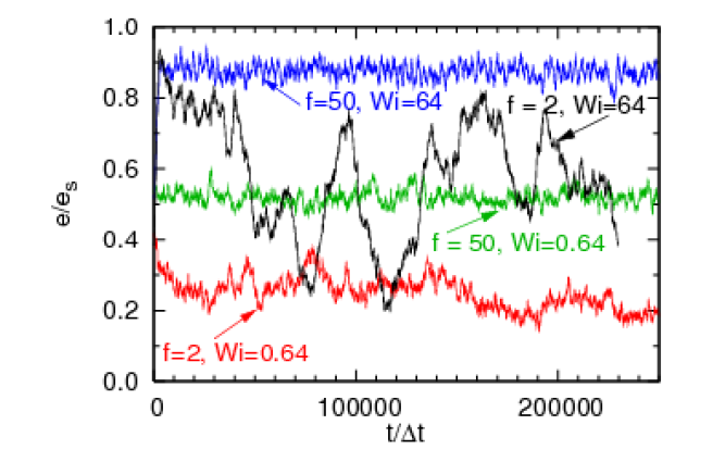
Figure 18: Temporal evolution of the largest intramolecular distance $e=\max_{ij}|{\bf r}_{i}-{\bf r}_{j}|$ of a linear polymer and a star polymer with $50$ arms, for the Weissenberg numbers $\rm Wi=0.64$ and $\rm Wi=64$. In both cases, $L_{f}=40$. The time $t$ is measured in units of the collision time $\delta t$. $e_{s}$ corresponds to the fully stretched arms. From Ref. ripo:06 .

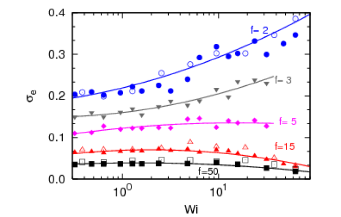
Figure 19: Widths of the distribution functions of the largest intramolecular distances, $\sigma_{e}=(\langle e^{2}\rangle-\langle e\rangle^{2})/\langle e\rangle^{2}$, of a linear polymer and star polymers with up to $50$ arms as a function of the Weissenberg number. From Ref. ripo:06 .

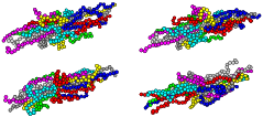
Figure 20: Successive snapshots of a star polymer of functionality $f=25$ and arm length $L_{f}=20$, which illustrate the tank-treating motion.

The rotational dynamics of a star polymer can be characterized quantitatively by calculating the rotation frequency

$$\omega_{\alpha}=\sum_{\beta=x}^{z}\langle\Theta_{\alpha\beta}^{-1}L_{\beta}\rangle$$ (96)

of a star, where

$$\Theta_{\alpha\beta}=\sum_{i=1}^{N_{m}}[{\vec{r}^{\prime}}_{i}^{2}\delta_{\alpha\beta}-r^{\prime}_{i,\alpha}r^{\prime}_{i,\beta}]$$ (97)

is the instantaneous moment-of-inertia tensor and $L_{\beta}$ is the instantaneous angular momentum. Since the rotation frequency for all kinds of soft objects—such as rods, linear polymers, droplets and capsules—depends linearly on $\dot{\gamma}$ for small shear rates, the reduced rotation frequency $\omega/{\dot{\gamma}}$ is shown in Fig. 21 as a function of the Weissenberg number. The data approach $\omega/{\dot{\gamma}}=1/2$ for small $\rm Wi$, as expected aust:99 ; aust:02 . For larger shear rates, the reduced frequency decreases due to the deformation and alignment of the polymers in the flow field. With increasing arm number, the decrease of $\omega/{\dot{\gamma}}$ at a given Weissenberg number becomes smaller, since the deviation from the spherical shape decreases. Remarkably, the frequency curves for all stars with $f>5$ are found to collapse onto a universal scaling function when $\omega/{\dot{\gamma}}$ is plotted as a function of a rescaled Weissenberg number, see Fig. 21. For high shear rates, $\omega/{\dot{\gamma}}$ decays as ${\rm Wi}^{-1}$, which implies that the rotation frequency becomes independent of $\dot{\gamma}$. A similar behavior has been observed for capsules at high shear rates navo:98 .

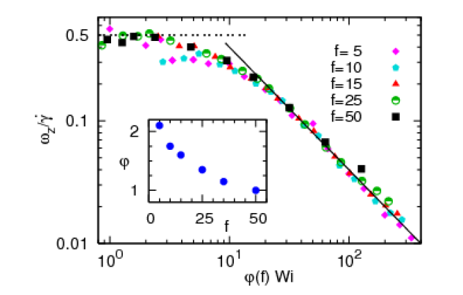
Figure 21: Scaled rotation frequencies as function of a rescaled Weissenberg number for various functionalities. Dashed and full lines correspond to $\omega/{\dot{\gamma}}=1/2$ for small $\rm Wi$, and $\omega/{\dot{\gamma}}\sim 1/{\rm Wi}$ for large $\rm Wi$, respectively. The inset shows the dependence of the rescaling factor $\varphi$ on the functionality. From Ref. ripo:06 .

The presented results show that star polymers in shear flow show a very rich structural and dynamical behavior. With increasing functionality, stars in flow change from linear-polymer-like to capsule-like behavior. These macromolecules are therefore interesting candidates to tune the viscoelastic properties of complex fluids.

11 Vesicles and Cells in Hydrodynamic Flows

11.1 Introduction

The flow behavior of fluid droplets, capsules, vesicles and cells is of enormous importance in science and technology. For example, the coalescence and break-up of fluid droplets is essential for emulsion formation and stability. Capsules and vesicles are discussed and used as drug carriers. Red blood cells (RBC) flow in the blood stream, and may coagulate or be torn apart under unfavorable flow conditions. Red blood cells also have to squeeze through narrow capillaries to deliver their oxygen cargo. White blood cells in capillary flow adhere to, roll along and detach again from the walls of blood vessels under normal physiological conditions; in inflamed tissue, leukocyte rolling leads to firm adhesion and induces an immunological response.

These and many other applications have induced an intensive theoretical and simulation activity to understand and predict the behavior of such soft, deformable objects in flow. In fact, there are some general, qualitative properties in simple shear flow, which are shared by droplets, capsules, vesicles and cells. When the internal viscosity is low and when they are highly deformable, a tank-treading motion is observed (in the case of droplets for not too high shear rates), where the shape and orientation are stationary, but particles localized at the interface or attached to the membrane orbit around the center of mass with a rotation axis in the vorticity direction. On the other hand, for high internal viscosity or small deformability, the whole object performs a tumbling motion, very much like a colloidal rod in shear flow. However, if we take a more careful look, then the behavior of droplets, capsules, vesicles and cells is quite different. For example, droplets can break up easily at higher shear rates, because their shape is determined by the interfacial tension; fluid vesicles can deform much more easily then capsules, since their membrane has no shear elasticity; etc. We focus here on the behavior of fluid vesicles and red blood cells.

11.2 Modeling Membranes

11.2.1 Modeling Lipid-Bilayer Membranes

The modeling of lipid bilayer membranes depends very much on the length scale of interest. The structure of the bilayer itself or the embedding of membrane proteins in a bilayer are best studied with atomistic models of both lipid and water molecules. Molecular dynamics simulations of such models are restricted to about $10^{3}$ lipid molecules. For larger system sizes, coarse-grained models are required goet98 ; gg:gomp99a ; otte03 . Here, the hydrocarbon chains of lipid molecules are described by short polymer chains of Lennard-Jones particles, which have a repulsive interaction with the lipid head groups as well as with the water molecules, which are also modeled as single Lennard-Jones spheres. Very similar models, with Lennard-Jones interactions replaced by linear “soft” dissipative-particle dynamics (DPD) potentials, have also been employed intensively shil02 ; rekv04 ; lara04 ; orti05 ; vent06 . For the investigation of shapes and thermal fluctuations of single- or multi-component membranes, the hydrodynamics of the solvent is irrelevant. In this case, it can be advantageous to use a solvent-free membrane model, in which the hydrophobic effect of the water molecules is replaced by an effective attraction among the hydrocarbon chains nogu01b ; nogu02c ; fara03 ; cook05a . This approach is advantageous in the case of membranes in dilute solution, because it reduces the number of molecules—and thus the degrees of freedom to be simulated—by orders of magnitude. However, it should be noticed that the basic length scale of atomistic and coarse-grained or solvent-free models is still on the same order of magnitude.

In order to simulate larger systems, such as giant unilamellar vesicles (GUV) or red blood cells (RBC), which have a radius on the order of several micrometers, a different approach is required. It has been shown that in this limit the properties of lipid bilayer membranes are described very well by modeling the membrane as a two-dimensional manifold embedded in three-dimensional space, with the shape and fluctuations controlled by the curvature elasticity helf73 ,

$${\cal H}=\int dS\ 2\kappa H^{2}\ ,$$ (98)

where $H=(c_{1}+c_{2})/2$ is the mean curvature, with the local principal curvatures $c_{1}$ and $c_{2}$, and the integral is over the whole membrane area. To make the curvature elasticity amenable to computer simulations, it has to be discretized. This can be done either by using triangulated surfaces gg:gomp97f ; gg:gomp04c , or by employing particles with properly designed interactions which favor the formation of self-assembled, nearly planar sheets drou91 ; nogu06 . In the latter case, both scalar particles with isotropic multi-particle interactions (and a curvature energy obtained from a moving least-squares method) nogu06 as well as particles with an internal spin variable and anisotropic, multi-body forces drou91 have been employed and investigated.

11.2.2 Dynamically Triangulated Surfaces

In a dynamically-triangulated surface model ho90 ; gg:gomp92a ; boal92a ; gg:gomp97f ; gg:gomp04c of vesicles and cells, the membrane is described by $N_{mb}$ vertices which are connected by tethers to form a triangular network of spherical topology, see Fig. 22. The vertices have excluded volume and mass $m_{mb}$. Two vertices connected by a bond have an attractive interaction, which keeps their distance below a maximum separation $\ell_{0}$. A short-range repulsive interaction among all vertices makes the network self-avoiding and prevents very short bond lengths. The curvature energy can be discretized in different ways gg:gomp96b ; gg:gomp97f . In particular, the discretization itzy86 ; gg:gomp96b

$$U_{cv}=\frac{\kappa}{2}\sum_{i}\frac{1}{\sigma_{i}}\left\{\sum_{j(i)}\frac{\sigma_{i,j}{\bf r}_{i,j}}{r_{i,j}}\right\}^{2}$$ (99)

has been found to give reliable results in comparison with the continuum expression (98). Here, the sum over $j(i)$ is over the neighbors of a vertex $i$ which are connected by tethers. The bond vector between the vertices $i$ and $j$ is ${\bf r}_{i,j}$, and $r_{i,j}=|{\bf r}_{i,j}|$. The length of a bond in the dual lattice is $\sigma_{i,j}=r_{i,j}[\cot(\theta_{1})+\cot(\theta_{2})]/2$, where the angles $\theta_{1}$ and $\theta_{2}$ are opposite to bond $ij$ in the two triangles sharing this bond. Finally, $\sigma_{i}=0.25\sum_{j(i)}\sigma_{i,j}r_{i,j}$ is the area of the dual cell of vertex $i$.

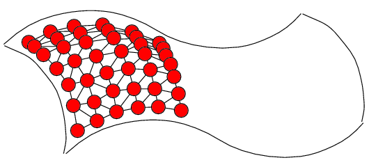
Figure 22: Triangulated-network model of a fluctuating membrane. All vertices have short-range repulsive interactions symbolized by hard spheres. Bonds represent attractive interactions with imply a maximum separation $\ell_{0}$ of connected vertices. From Ref. gomp02_FS .

To model the fluidity of the membrane, tethers can be flipped between the two possible diagonals of two adjacent triangles. A number $\psi N_{b}$ of bond-flip attempts is performed with the Metropolis Monte Carlo method gg:gomp96b at time intervals $\Delta t_{BF}$, where $N_{b}=3(N_{mb}-2)$ is the number of bonds in the network, and $0<\psi<1$ is a parameter of the model. Simulation results show that the vertices of a dynamically triangulated membrane show diffusion, i.e., the squared distance of two initially neighboring vertices increases linearly in time.

11.2.3 Vesicle Shapes

Since the solubility of lipids in water is very low, the number of lipid molecules in a membrane is essentially constant over typical experimental time scales. Also, the osmotic pressure generated by a small number of ions or macromolecules in solution, which cannot penetrate the lipid bilayer, keeps the internal volume essentially constant. The shape of fluid vesicles seif91b is therefore determined by the competition of the curvature elasticity of the membrane, and the constraints of constant volume $V$ and constant surface area $S$. In the simplest case of vanishing spontaneous curvature, the curvature elasticity is given by Eq. (98). In this case, the vesicle shape in the absence of thermal fluctuations depends on a single dimensionless parameter, the reduced volume $V^{*}=V/V_{0}$, where $V_{0}=(4\pi/3)R_{0}^{3}$ and $R_{0}=(S/4\pi)^{1/2}$ are the volume and radius of a sphere of the same surface area $S$, respectively. The calculated vesicle shapes are shown in Fig. 23. There are three phases. For reduced volumes not too far from the sphere, elongated prolate shapes are stable. In a small range of reduced volumes of $V^{*}\in[0.592,0.651]$, oblate discocyte shapes have the lowest curvature energy. Finally, at very low reduced volumes, cup-like stomatocyte shapes are found.

These shapes are very well reproduced in simulations with dynamically triangulated surfaces gg:gomp94k ; gg:gomp95a ; gg:gomp03c ; nogu_05_dfv .

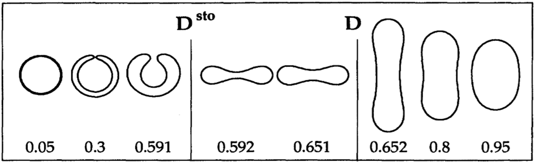
Figure 23: Shapes of fluid vesicles as a function of the reduced volume $V^{*}$. $D$ and $D^{sto}$ denote the discontinuous prolate-oblate and oblate-stomatocyte transitions, respectively. All shapes display rotational symmetry with respect to the vertical axis. From Ref. seif91b .

11.2.4 Modeling Red Blood Cells

Red blood cells have a biconcave disc shape, which can hardly be distinguished from the discocyte shape of fluid vesicles with reduced volume $V^{*}\simeq 0.6$, compare Fig. 23. However, the membrane of red blood cells is more complex, since a spectrin network is attached to the plasma membrane albe07 , which helps to retain the integrity of the cell in strong shear gradients or capillary flow. Due to the spectrin network, the red blood cell membrane has a non-zero shear modulus $\mu$.

The bending rigidity $\kappa$ of RBCs has been measured by micropipette aspiration moha94 and atomic force microscopy sche01 to be approximately $\kappa=50k_{B}T$. The shear modulus of the composite membrane, which is induced by the spectrin network, has been determined by several techniques; it is found to be $\mu=2\times 10^{-6}$ N/m from optical tweezers manipulation leno01 , while the value $\mu=6\times 10^{-6}$ N/m is obtained from micropipette aspiration moha94 . Thus, the dimensionless ratio $\mu R_{0}^{2}/\kappa\simeq 100$, which implies that bending and stretching energies are roughly of equal importance.

Theoretically, the shapes of RBCs in the absence of flow have been calculated very successfully on the basis of a mechanical model of membranes, which includes both curvature and shear elasticity disc98 ; lim02 . In particular, it has been shown recently that the full stomatocyte-discocyte-echinocyte sequence of RBCs can be reproduced by this model lim02 .

The composite membrane of a red blood cell, consisting of the lipid bilayer and the spectrin network, can be modeled as a composite network, which consists of a dynamically-triangulated surface as in the case of fluid vesicles, coupled to an additional network of harmonic springs with fixed connectivity (no bond-flip) disc98 ; gg:gomp05g . Ideally, the bond length of the elastic network is larger than of the fluid mesh disc98 —in order to mimic the situation of the red blood cell membrane, where the average distance of anchoring points is about 70 nm, much larger than the size of a lipid molecule—and thereby allow, for example, for thermal fluctuations of the distances between neighboring anchoring points. On the other hand, to investigate the behavior of cells on length scales much larger the mesh size of the spectrin network, it is more efficient to use the same number of the bonds for both the fluid and the tethered networks gg:gomp05g . The simplest case is a harmonic tethering potential, $(1/2)k_{\rm{el}}({\bf r}_{i}-{\bf r}_{j})^{2}$. This tether network generates a shear modulus $\mu=\sqrt{3}k_{\rm{el}}$.

11.3 Modeling Membrane Hydrodynamics

Solvent-free models, triangulated surfaces and other discretized curvature models have the disadvantage that they do not contain a solvent, and therefore do not describe the hydrodynamic behavior correctly. However, this apparent disadvantage can be turned into an advantage by combining these models with a mesoscopic hydrodynamics technique. This approach has been employed for dynamically triangulated surfaces nogu_04_fvv ; nogu_05_dfv and for meshless membrane models in combination with MPC gg:gomp06h , as well as for fixed membrane triangulations in combination with both MPC gg:gomp05g and the Lattice Boltzmann method (LBM) dupi07 .

The solvent particles of the MPC fluid interact with the membrane in two ways to obtain an impermeable membrane with no-slip boundary conditions. First, the membrane vertices are included in the MPC collision procedure, as suggested for polymers in Ref. male_00_dsp , compare Sec. 7.1. Second, the solvent particles are scattered with a bounce-back rule from the membrane surface. Here, solvent particles inside ($1\leq i\leq N_{in}$) and outside ($N_{in}<i\leq N_{s}$) of the vesicle have to be distinguished. The membrane triangles are assumed to have a finite but very small thickness $\delta=2l_{bs}$. The scattering process is then performed at discrete time steps $\Delta t_{BS}$, so that scattering does not occur exactly on the membrane surface, but the solvent particles can penetrate slightly into the membrane film nogu_05_dfv . A similar procedure has bee suggested in Ref. kiku_03_tcm for spherical colloidal particles embedded in a MPC solvent. Particles which enter the membrane film, i.e., which have a distance to the triangulated surface smaller than $l_{bs}$, or interior particles which reach the exterior volume and vice versa, are scattered at the membrane triangle with the closest center of mass. Explicitly nogu_05_dfv ,

$${\bf v}^{(new)}_{s}(t) = {\bf v}_{s}(t)-\frac{6m_{mb}}{m_{s}+3m_{mb}}({\bf v}_{s}(t)-{\bf v}_{tri}(t))$$ (100)

$${\bf v}^{(new)}_{tri}(t) = {\bf v}_{tri}(t)+\frac{2m_{s}}{m_{s}+3m_{mb}}({\bf v}_{s}(t)-{\bf v}_{tri}(t)),$$ (101)

when $({\bf v}_{s}(t)-{\bf v}_{tri}(t))\cdot{\bf n}_{tri}<0$, where ${\bf v}_{s}(t)$ and ${\bf v}_{tri}(t)$ are the velocities of the solvent particle and of the center of mass of the membrane triangle, respectively, and ${\bf n}_{tri}$ is the normal vector of the triangle, which is oriented towards the outside (inside) for external (internal) particles.

The bond flips provide a very convenient way to vary the membrane viscosity $\eta_{mb}$, which increases with decreasing probability $\psi$ for the selection of a bond for a bond-flip attempt. The membrane viscosity has been determined quantitatively from a simulation of a flat membrane in two-dimensional Poiseuille flow. The triangulated membrane is put in a rectangular box of size $L_{x}\times L_{y}$ with periodic boundary conditions in the $x$-direction. The edge vertices at the lower and upper boundary ($y=\pm L_{y}/2$) are fixed at their positions. A gravitational force $(m_{mb}g,0)$ is applied to all membrane vertices to induce a flow. Rescaling of relative velocities is employed as a thermostat. Then, the membrane viscosity is calculated from $\eta_{mb}=\rho_{mb}gL_{y}/8v_{max}$, where $\rho_{mb}$ is average mass density of the membrane particles, and $v_{max}$ the maximum velocity of the parabolic flow profile. The membrane viscosity $\eta_{mb}$, which is obtained in this way, is shown in Fig. 24. As $\psi$ decreases, it takes longer and longer for a membrane particle to escape from the cage of its neighbors, and $\eta_{mb}$ increases. This is very similar to the behavior of a hard-sphere fluid with increasing density. Finally, for $\psi=0$, the membrane becomes solid.

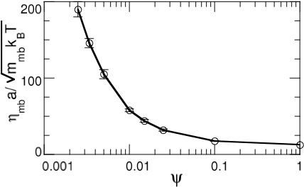
Figure 24: Dependence of the membrane viscosity $\eta_{mb}$ on the probability $\psi$ for the selection of a bond for a bond-flip attempt, for a membrane with $N_{mb}=1860$ vertices. From Ref. nogu_05_dfv .

11.4 Fluid Vesicles in Shear Flow

The dynamical behavior of fluid vesicles in simple shear flow has been studied experimentally haas97 ; kant05 ; kant06 ; made06 , theoretically kell82 ; seco82 ; seco83 ; tran84 ; seif99b ; misb06 ; dank07b ; lebe07 , numerically with the boundary-integral technique krau96 ; beau04b or the phase-field method beau04b ; bibe05 , and with mesoscale solvents nogu_04_fvv ; nogu_05_dfv ; gg:gomp07c . The vesicle shape is now determined by the competition of the curvature elasticity of the membrane, the constraints of constant volume $V$ and constant surface area $S$, and the external hydrodynamic forces.

Shear flow is characterized (in the absence of vesicles or cells) by the flow field ${\bf v}=\dot{\gamma}y{\bf e}_{x}$, where ${\bf e}_{x}$ is a unit vector, compare Sec. 10.4. The control parameter of shear flow is the shear rate $\dot{\gamma}$, which has the dimension of an inverse time. Thus, a dimensionless, scaled shear rate $\dot{\gamma}^{*}=\dot{\gamma}\tau$ can be defined, where $\tau$ is the longest relaxation time of a vesicle. It is given by $\tau=\eta_{0}R_{0}^{3}/\kappa$, where $\eta_{0}$ is the solvent viscosity, $R_{0}$ the average radius, and $\kappa$ the bending rigidity broc75 . For $\dot{\gamma}^{*}<1$, the internal vesicle dynamics is fast compared to the external perturbation, so that the vesicle shape is hardly affected by the flow field, whereas for $\dot{\gamma}^{*}>1$, the flow forces dominate and the vesicle is in a non-equilibrium steady state.

One of the difficulties in theoretical studies of the hydrodynamic effects on vesicle dynamics is the no-slip boundary condition for the embedding fluid on the vesicle surface, which changes its shape dynamically under the effect of flow and curvature forces. In early studies, a fluid vesicle was therefore modeled as an ellipsoid with fixed shape kell82 . This simplified model is still very useful as a reference for the interpretation of simulation results.

11.4.1 Generalized Keller-Skalak Theory

The theory of Keller and Skalak kell82 describes the hydrodynamic behavior of vesicles of fixed ellipsoidal shape in shear flow, with the viscosities $\eta_{in}$ and $\eta_{0}$ of the internal and external fluids, respectively. Despite of the approximations needed to derive the equation of motion for the inclination angle $\theta$, which measures the deviation of the symmetry axis of the ellipsoid with the flow direction, this theory describes vesicles in flow surprisingly well. It has been generalized later tran84 to describe the effects of a membrane viscosity $\eta_{mb}$.

The main result of the theory of Keller and Skalak is the equation of motion for the inclination angle kell82 ,

$$\frac{d}{dt}{\theta}=\frac{1}{2}\dot{\gamma}\{-1+B\cos(2\theta)\},$$ (102)

where $B$ is a constant, which depends on the geometrical parameters of the ellipsoid, on the viscosity contrast $\eta_{in}^{*}=\eta_{in}/\eta_{0}$, and the scaled membrane viscosity $\eta_{mb}^{*}=\eta_{mb}/(\eta_{0}R_{0})$ kell82 ; tran84 ; nogu_05_dfv ,

$$B=f_{0}\left\{f_{1}+\frac{f_{1}^{-1}}{1+f_{2}(\eta_{in}^{*}-1)+f_{2}f_{3}\eta_{mb}^{*}}\right\},$$ (103)

where $f_{0}$, $f_{1}$, $f_{2}$, and $f_{3}$ are geometry-dependent parameters. In the spherical limit, $B\to\infty$. Eq. (102) implies the following behavior:

• For $B>1$, there is a stationary solution, with $\cos(2\theta)=1/B$. This corresponds to a tank-treading motion, in which the orientation of the vesicle axis is time independent, but the membrane itself rotates around the vorticity axis.

• For $B<1$, no stationary solution exists, and the vesicle shows a tumbling motion, very similar to a solid rod-like colloidal particle in shear flow.

• The shear rate $\dot{\gamma}$ only determines the time scale, but does not affect the tank-treading or tumbling behavior. Therefore, a transition between these two types of motion can only be induced by a variation of the vesicle shape or the viscosities.

However, the vesicle shape in shear flow is often not as constant as assumed by Keller and Skalak. In these situations, it is very helpful to compare simulation results with a generalized Keller-Skalak theory, in which shape deformation and thermal fluctuations are taken into account. Therefore, a phenomenological model has been suggested in Ref. nogu_05_dfv , in which in addition to the inclination angle $\theta$ a second parameter is introduced to characterize the vesicle shape and deformation, the asphericity rudn86

$$\alpha=\frac{({\lambda_{1}}-{\lambda_{2}})^{2}+({\lambda_{2}}-{\lambda_{3}})^{2}+({\lambda_{3}}-{\lambda_{1}})^{2}}{2R_{g}^{4}},$$ (104)

where ${\lambda_{1}}\leq{\lambda_{2}}\leq{\lambda_{3}}$ are the eigenvalues of the moment-of-inertia tensor and the squared radius of gyration $R_{g}^{2}=\lambda_{1}+\lambda_{2}+\lambda_{3}$. This implies $\alpha=0$ for spheres (with $\lambda_{1}={\lambda_{2}}={\lambda_{3}}$), $\alpha=1$ for long rods (with $\lambda_{1}={\lambda_{2}}\ll{\lambda_{3}}$), and $\alpha=1/4$ for flat disks (with $\lambda_{1}\ll{\lambda_{2}}={\lambda_{3}}$). The generalized Keller-Skalak model is then defined by the stochastic equations

$$\zeta_{\alpha}\frac{d}{dt}{\alpha}=-\partial F/\partial\alpha+{A}\dot{\gamma}\sin(2\theta)+\zeta_{\alpha}g_{\alpha}(t)$$ (105)

$$\frac{d}{dt}{\theta}=\frac{1}{2}\dot{\gamma}\{-1+B(\alpha)\cos(2\theta)\}+g_{\theta}(t),$$ (106)

with Gaussian white noises $g_{\alpha}$ and $g_{\theta}$, which are determined by

$$\langle g_{\alpha}(t)\rangle=\langle g_{\theta}(t)\rangle = \langle g_{\alpha}(t)g_{\theta}(t^{\prime})\rangle=0,$$

$$\langle g_{\alpha}(t)g_{\alpha}(t^{\prime})\rangle = 2D_{\alpha}\delta(t-t^{\prime}),$$ (107)

$$\langle g_{\theta}(t)g_{\theta}(t^{\prime})\rangle = 2D_{\theta}\delta(t-t^{\prime}),$$

friction coefficients $\zeta_{\alpha}$ and $\zeta_{\theta}$, and diffusion constants $D_{\alpha}=k_{\rm B}T/\zeta_{\alpha}$ and $D_{\theta}=k_{\rm B}T/\zeta_{\theta}$. Note that $\zeta_{\theta}$ does not appear in Eq. (106); it drops out because the shear force is also caused by friction.

The form of the stochastic equations (105) and (106) is motivated by the following considerations. The first term in Eq. (105), $\partial F/\partial\alpha$, is the thermodynamic force due to bending energy and volume constraints; it is calculated from the free energy $F(\alpha)$. The second term of Eq. (105) is the deformation force due to the shear flow. Since the hydrodynamic forces elongate the vesicle for $0<\theta<\pi/2$ but push to reduce the elongation for $-\pi/2<\theta<0$, the flow forces should be proportional to $\sin(2\theta)$ to leading order. The amplitude $A$ is assumed to be independent of the asphericity $\alpha$. $\zeta_{\alpha}$ and $A$ can be estimated gg:gomp07c from the results of a perturbation theory misb06 in the quasi-spherical limit. Eq. (106) is adapted from Keller-Skalak theory. While $B$ is a constant in Keller-Skalak theory, it is now a function of the (time-dependent) asphericity $\alpha$ in Eq. (106).

11.4.2 Effects of Membrane Viscosity: Tank-Treading and Tumbling

The theory of Keller and Skalak kell82 predicts for fluid vesicles a transition from tank-treading to tumbling with increasing viscosity contrast $\eta_{in}/\eta_{0}$. This has been confirmed in recent simulations based on a phase-field model beau04b .

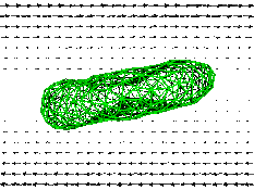
Figure 25: Snapshot of a discocyte vesicle in shear flow with reduced shear rate $\dot{\gamma}^{*}=0.92$, reduced volume $V^{*}=0.59$, membrane viscosity $\eta_{mb}^{*}=0$ and viscosity contrast $\eta_{in}/\eta_{0}=1$. The arrows represent the velocity field in the $xz$-plane. From Ref. nogu_05_dfv .

The membrane viscosity $\eta_{mb}$ is also an important factor for the vesicle dynamics in shear flow. For example, the membrane of red blood cells becomes more viscous on aging tran84 ; nash83 or in diabetes mellitus tsuk01 . Experiments indicate that the energy dissipation in the membrane is larger than that inside a red blood cell seco83 ; tran84 . Furthermore, it has been shown recently that vesicles can not only be made from lipid bilayers, but also from bilayers of block copolymers disc99 . The membrane viscosity of these “polymersomes” is several orders of magnitude larger than for liposomes, and can be changed over a wide range by varying the polymer chain length dimo02 .

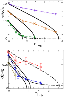
Figure 26: Average inclination angle $\langle\theta\rangle$ as a function of reduced membrane viscosity $\eta_{mb}^{*}$, for the shear rate $\dot{\gamma}^{*}=0.92$ and various reduced volumes $V^{*}$. Results are presented for prolate (circles) and discocyte (squares) vesicles with $V^{*}=0.59$, as well as prolate vesicles with $V^{*}=0.66$ (triangles), $0.78$ (diamonds), $0.91$ (crosses), and $V^{*}=0.96$ (pluses). The solid and dashed lines are calculated by K-S theory, Eqs. (102) and (103), for prolate ($V^{*}=0.59$, $0.66$, $0.78$, $0.91$, and $0.96$) and oblate ellipsoids ($V^{*}=0.59$), respectively. The dashed-dotted lines are calculated from Eq. (106) with thermal fluctuations, for $V^{*}=0.66$, $V^{*}=0.78$, and the rotational Peclet number $\dot{\gamma}/D_{\theta}=600$ (where $D_{\theta}$ is the rotational diffusion constant). From Ref. nogu_05_dfv .

A variation of the membrane viscosity can be implemented easily in dynamically triangulated surface models of membranes, as explained in Sec. 11.2.2. An example of a discocyte in tank-treading motion, which is obtained by such a membrane model nogu_05_dfv , is shown in Fig. 25. Simulation results for the inclination angle as a function of the reduced membrane viscosity $\eta^{*}_{mb}=\eta_{mb}/(\eta_{0}R_{0})$ are shown in Fig. 26. This demonstrates the tank-treading to tumbling transition of fluid vesicles with increasing membrane viscosity. The threshold shear rate decreases with decreasing reduced volume $V^{*}$, since with increasing deviation from the spherical shape, the energy dissipation within the membrane increases. Interestingly, the discocyte shape is less affected by the membrane viscosity than the prolate shape for $V^{*}=0.59$, since it is more compact—in contrast to a vesicle with viscosity contrast $\eta_{in}/\eta_{0}>1$, where the prolate shape is affected less nogu_05_dfv .

Figure 26 also shows a comparison of the simulation data with results of K-S theory for fixed shape, both without and with thermal fluctuations. Note that there are no adjustable parameters. The agreement of the results of theory and simulations is excellent in the case of vanishing membrane viscosity, $\eta_{mb}=0$. For small reduced volumes, $V^{*}\simeq 0.6$, the tank-treading to tumbling transition is smeared out by thermal fluctuations, with an intermittent tumbling motion occurring in the crossover region. This behavior is captured very well by the generalized K-S model with thermal fluctuations. For larger reduced volumes and non-zero membrane viscosity, significant deviations of theory and simulations become visible. The inclination angle $\theta$ is found to decrease much more slowly with increasing membrane viscosity than expected theoretically. This is most likely due to thermal membrane undulations, which are not taken into account in K-S theory.

11.4.3 Swinging of Fluid Vesicles

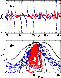
Figure 27: Temporal evolution of vesicle deformation $\alpha_{D}$ and inclination angle $\theta$, for $V^{*}=0.78$ and $\eta_{mb}^{*}=2.9$. Here, $\alpha_{D}=(L_{1}-L_{2})/(L_{1}+L_{2})$, where $L_{1}$ and $L_{2}$ are the maximum lengths in the direction of the eigenvectors of the gyration tensor in the vorticity plane. The solid (red) and dashed (blue) lines represent simulation data for $\dot{\gamma}^{*}=3.68$ and $0.92$ ($\kappa/k_{B}T=10$ and $40$, with $\dot{\gamma}\eta_{0}R_{0}^{3}/k_{B}T=36.8$), respectively. The solid lines in (b) are obtained from Eqs. (105), (106) without thermal noise for $\dot{\gamma}^{*}=1.8$, $3.0$, and $10$ (from top to bottom). From Ref. gg:gomp07c .

Recently, of a new type of vesicle dynamics in shear flow has been observed experimentally kant06 , which is characterized by oscillations of the inclination angle $\theta$ with $\theta(t)\in[-\theta_{0},\theta_{0}$] and $\theta_{0}<\pi/2$. The vesicles were found to transit from tumbling to this oscillatory motion with increasing shear rate $\dot{\gamma}$. Simultaneously with the experiment, a “vacillating-breathing” mode for quasi-spherical fluid vesicles was predicted theoretically, based on a spherical-harmonics expansion of the equations of motion to leading order (without thermal fluctuations) misb06 . This mode exhibits similar dynamical behavior as seen experimentally; however, it “coexists” with the tumbling mode, and its orbit depends on the initial deformation, i.e., it is not a limit cycle. Furthermore, the shear rate appears only as the basic time scale, and therefore cannot induce any shape transitions. Hence it does not explain the tumbling-to-oscillatory transition seen in the experiments kant06 .

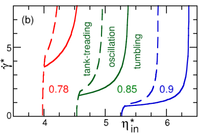
Figure 28: Dynamical phase diagram as a function of viscosity contrast $\eta_{in}^{*}=\eta_{in}/\eta_{0}$, for $\eta_{\rm{mb}}^{*}=0$ and various reduced volumes $V^{*}$, calculated from Eqs. (105), (106) without thermal noise. The tank-treading phase is located on the left-hand-side of the dashed lines. The solid lines represent the tumbling-to-swinging transitions. From Ref. gg:gomp07c .

Simulation data for the oscillatory mode—which has also been denoted “trembling” kant06 or “swinging” gg:gomp07c mode—are shown in Fig. 27. The simulation results demonstrate that the transition can indeed be induced by increasing shear rate, and that it is robust to thermal fluctuations. Figure 27 also shows that the simulation data are well captured by the generalized K-S model, Eqs. (105) and (106), which takes into account higher-order contributions in the curvature energy of a vesicle. The theoretical model can therefore be used to predict the full dynamic phase diagram of prolate vesicles as a function of shear rate and membrane viscosity or viscosity contrast, compare Fig. 28. The swinging phase appears at the boundary between the tank-treading and the tumbling phase for sufficiently large shear rates. The phase diagram explains under which conditions the swinging phase can be reached from the tumbling phase with increasing shear rate—as observed experimentally kant06 .

The generalized K-S model is designed to capture the vesicle flow behavior for non-spherical shapes sufficiently far from a sphere. For quasi-spherical vesicles, a derivation of the equations of motion by a systematic expansion in the undulation amplitudes gives quantitatively more reliable results. An expansion to third order results in a phase diagram dank07b ; lebe07 , which agrees very well with Fig. 28.

11.4.4 Flow-Induced Shape Transformations

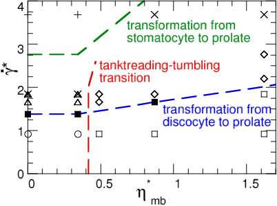
Figure 29: Dynamical phase diagram of a vesicle in shear flow for reduced volume $V^{*}=0.59$. Symbols show simulated parameter values, and indicate tank-treading discocyte and tank-treading prolate ($\circ$), tank-treading prolate and unstable discocyte ($\triangle$), tank-treading discocyte and tumbling (transient) prolate ($\square$), tumbling with shape oscillation ($\diamond$), unstable stomatocyte ($+$), stable stomatocyte ($\times$), and near transition ($\blacksquare$). The dashed lines are guides to the eye. From Ref. nogu_05_dfv .

Shear flow does not only induce different dynamical modes of prolate and oblate fluid vesicles, it can also induce phase transformations. The simplest case is a oblate fluid vesicle with $\eta_{mb}=0$ and viscosity contrast $\eta_{in}/\eta_{0}=1$. When the reduced shear rate reaches $\dot{\gamma}^{*}\simeq 1$, the discocyte vesicles are stretched by the flow forces into a prolate shape krau96 ; nogu_04_fvv ; nogu_05_dfv . A similar transition is found for stomatocyte vesicles, except that in this case a larger shear rate $\dot{\gamma}^{*}\simeq 3$ is required. In the case of non-zero membrane viscosity, a rich phase behavior appears, see Fig. 29.

Surprisingly, flow forces can not only stretch vesicles into a more elongated shape, but can also induce a transition from an elongated prolate shape into a more compact discocyte shape nogu_05_dfv . Simulation results for the latter transition are shown in Fig. 30. This transition is possible, because in a range of membrane viscosities, the prolate shape is in the tumbling phase, while the oblate shape is tank-treading, compare Fig. 26. Of course, this requires that the free energies of the two shapes are nearly equal, which implies a reduced volume of $V^{*}\simeq 0.6$. Thus, a prolate vesicle in this regime starts tumbling; as the inclination angle becomes negative, shear forces push to shrink the long axis of the vesicle; when this force is strong enough to overcome the free-energy barrier between the prolate and the oblate phase, a shape transformation can be induced, compare Fig. 30. The vesicle then remains in the stable tank-treading state.

At higher shear rates, on intermittent behavior has been observed, in which the vesicle motion changes in irregular intervals between tumbling and tank-treading nogu_05_dfv .

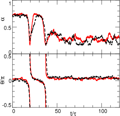
Figure 30: Time dependence of asphericity $\alpha$ and inclination angle $\theta$, for $\dot{\gamma}^{*}=1.84$, $\eta_{\rm{mb}}^{*}=1.62$, and $V^{*}=0.59$. The dashed lines are obtained from Eqs. (105) and (106), with $\zeta_{\alpha}=100$, $A=12$, and $B(\alpha)=1.1-0.17\alpha$. From Ref. gg:gomp05i .

11.4.5 Vesicle Fluctuations under Flow in Two Dimensions

At finite temperature, stochastic fluctuations of the membrane due to thermal motion affect the dynamics of vesicles. Since the calculation of thermal fluctuations under flow conditions requires long times and large membrane sizes (in order to have a sufficient range of undulation wave vectors), simulations have been performed for a two-dimensional system in the stationary tank-treading state gg:gomp08xxc . For comparison, in the limit of small deformations from a circle, Langevin-type equations of motion have been derived, which are highly nonlinear due to the constraint of constant perimeter length gg:gomp08xxc .

The effect of the shear flow is to induce a tension in the membrane, which reduces the amplitude of thermal membrane undulations. This tension can be extracted directly from simulation data for the undulation spectrum. The reduction of the undulation amplitudes also implies that the fluctuations of the inclination angle $\theta$ get reduced with increasing shear rate. The theory for quasi-circular shapes predicts a universal behavior as a function of the scaled shear rate $\dot{\gamma}^{*}\Delta^{1/2}\kappa/(R_{0}k_{B}T)$, where $\dot{\gamma}^{*}=\dot{\gamma}\eta_{0}R_{0}^{3}/\kappa$ is the reduced shear rate in two dimensions, and $\Delta$ is the dimensionless excess membrane length. Theory and simulation results for the inclination angle as a function of the reduced shear rate are shown in Fig. 31. There are no adjustable parameters. The agreement is excellent as long as the deviations from the circular shape are not too large gg:gomp08xxc .

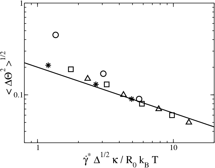
Figure 31: Fluctuations of the inclination angle $\langle\Delta\theta^{2}\rangle^{1/2}$ of a two-dimensional fluctuating vesicle in shear flow, as a function of scaled shear rate $\dot{\gamma}^{*}\Delta^{1/2}\kappa/(R_{0}k_{B}T)$, where $\Delta$ is the dimensionless excess membrane length. Symbols indicate simulation data for different internal vesicle areas $A$ for fixed membrane length, with $A^{*}\equiv A/\pi R_{0}^{2}=0.95$ (squares), $A^{*}=0.90$ (triangles), $A^{*}=0.85$ (stars), and $A^{*}=0.7$ (circles). The solid line is the theoretical result in the quasi-circular limit. From Ref. gg:gomp08xxc .

11.5 Fluid Vesicles and Red Blood Cells in Capillary Flow

11.5.1 RBC Deformation in Narrow Capillaries

The deformation of single RBCs and single fluid vesicles in capillary flows were studied theoretically by lubrication theories seco86 ; skal90 ; brui96 and boundary-integral methods queg97 ; pozr05a ; pozr05b . In most of these studies, axisymmetric shapes which are coaxial with the center of the capillary were assumed and cylindrical coordinates were employed. In order to investigate non-axisymmetric shapes as well as flow-induced shape transformations, a fully three-dimensional simulation approach is required.

We focus here on the behavior of single red blood cells in capillary flow gg:gomp05g , as described by a triangulated surface model for the membrane (compare Sec. 11.2.4) immersed in a MPC solvent (see Sec. 11.2.4). The radius of the capillary, $R_{cap}$, is taken to be slightly larger than the mean vesicle or RBC radius, $R_{0}=\sqrt{S/4\pi}$, where $S$ is the membrane area. Snapshots of vesicle and RBC shapes in flow are shown in Fig. 32 for a reduced volume of $V^{*}=0.59$, where the vesicle shape at rest is a discocyte. For sufficiently small flow velocities, the discocyte shape is retained. However, the discocyte is found not in a coaxial orientation; instead the shortest eigenvalue of the gyration tensor is oriented perpendicular to the cylinder axis gg:gomp05g . Since two opposite sides of the rim of the discocyte are closer to wall where the flow velocity is small, the rotational symmetry is slightly disturbed and the top view looks somewhat triangular, see Fig. 32A. With increasing flow velocity, a shape transition to an axisymmetric shape occurs. In the case of fluid vesicles this is a prolate shape, while in the case of RBCs a parachute shape is found. Such parachute shapes of red blood cells have previously been observed experimentally skal69 ; tsuk01 .

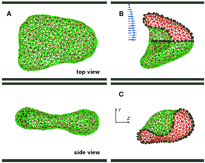
Figure 32: Snapshots of vesicles in capillary flow, with bending rigidity $\kappa/k_{B}T=20$ and capillary radius $R_{cap}=1.4R_{0}$. (A) Fluid vesicle with discoidal shape at the mean fluid velocity $v_{m}\tau/R_{cap}=41$, both in side and top views. (B) Elastic vesicle (RBC model) with parachute shape at $v_{m}\tau/R_{cap}=218$ (with shear modulus $\mu R_{0}^{2}/k_{B}T=110$). The blue arrows represent the velocity field of the solvent. (C) Elastic vesicle with slipper-like shape at $v_{m}\tau/R_{cap}=80$ (with $\mu R_{0}^{2}/k_{B}T=110$). The inside and outside of the membrane are depicted in red and green, respectively. The upper front quarter of the vesicle in (B) and the front half of the vesicle in (C) are removed to allow for a look into the interior; the black circles indicate the lines where the membrane has been cut in this procedure. Thick black lines indicate the walls the cylindrical capillary. From Ref. gg:gomp05g .

The fundamental difference between the flow behaviors of fluid vesicles and red blood cells at high flow velocities is due to the shear elasticity of the spectrin network. Its main effect for $\mu R_{0}^{2}/\kappa\gtrsim 1$ is to suppress the discocyte-to-prolate transition, because the prolate shape would acquire an elastic energy of order $\mu R_{0}^{2}$. In comparison, the shear stress in the parachute shape is much smaller.

Some diseases, such as diabetes mellitus and sickle cell anemia, change the mechanical properties of RBCs; a reduction of RBC deformability was found to be responsible for an enhanced flow resistance of blood chie87 . Therefore, it is very important to understand the relation of RBC elasticity and flow properties in capillaries. The flow velocity at the discocyte-to-prolate transition of fluid vesicles and at the discocyte-to-parachute transition is therefore shown in Fig. 33 as a function of the bending rigidity and the shear modulus, respectively. In both cases, an approximately linear dependence is obtained gg:gomp05g ,

$$v_{m}^{c}\frac{\tau}{R_{cap}}=0.1\frac{\mu R_{0}^{2}}{k_{B}T}+4.0\frac{\kappa}{k_{B}T}.$$ (108)

This result suggests that parachute shapes of RBCs should appear for flow velocities larger than $v_{m}^{c}=800R_{cap}/\tau$ $\simeq 0.2$mm/s under physiological conditions. This is consistent with the experimental results of Ref. suzu96 , and is in the range of micro-circulation in the human body.

Figure 33 (right) also shows that there is a metastable region, where discocytes are seen for increasing flow velocity, but parachute shapes for decreasing flow velocity. This hysteresis becomes more pronounced with increasing shear modulus. It is believed to be due to a suppression of thermal fluctuations with increasing $\mu R_{0}^{2}/k_{B}T$.

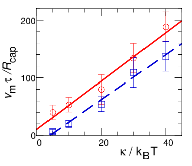
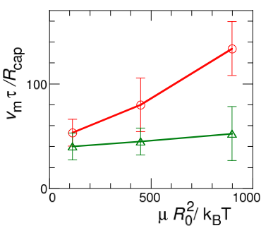
Figure 33: Critical flow velocity $v_{m}$ of the discocyte-to-parachute transition of elastic vesicles and of the discocyte-to-prolate transition of fluid vesicles, as a function of the bending rigidity $\kappa$. From Ref. gg:gomp05g .

11.5.2 Flow in Wider Capillaries

The flow of many red blood cells in wider capillaries has also been investigated by several simulation techniques. Discrete fluid-particle simulations—an extension of dissipative-particle dynamics (DPD)—in combination with bulk-elastic discocyte cells (in contrast to the membrane elasticity of real red blood cells) have been employed to investigate the dynamical clustering of red blood cells in capillary vessels bory03 ; dzwi03 . An immersed finite-element model—a combination of the immersed boundary method for the solvent hydrodynamics eggl98 and a finite-element method to describe the membrane elasticity—has been developed to study red blood cell aggregation liu06 . Finally, it has been demonstrated that the Lattice-Boltzmann method for the solvent in combination with a triangulated mesh model with curvature and shear elasticity for the membrane can be used efficiently to simulate RBC suspensions in wider capillaries dupi07 .

12 Viscoelastic Fluids

One of the unique properties of soft matter is its viscoelastic behavior lars_99_src . Due to the long structural relaxation times, the internal degrees of freedom cannot relax sufficiently fast in an oscillatory shear flow already at moderate frequencies, so that there is an elastic restoring force which pushes the system back to its previous state. Well studied examples of viscoelastic fluids are polymer solutions and polymer melts doi:86 ; lars_99_src .

The viscoelastic behavior of polymer solutions leads to many unusual flow phenomena, such as viscoelastic phase separation tana_00_vps . There is also a second level of complexity in soft matter systems, in which a colloidal component is dispersed in a solvent, which is itself a complex fluid. Examples are spherical or rod-like colloids dispersed in polymer solutions. Shear flow can induce particle aggregation and alignment in these systems verm_05_fis .

It is therefore desirable to generalize the MPC technique to model viscoelastic fluids, while retaining as much as possible of the computational simplicity of standard MPC for Newtonian fluids. This can be done by replacing the point particles of standard MPC by harmonic dumbbells with spring constant $K$ tao_08 .

As for point particles, the MPC algorithm consists of two steps, streaming and collisions. In the streaming step, within a time interval $\Delta t$, the motion of all dumbbells is governed by Newton’s equations of motion. The center-of-mass coordinate of each dumbbell follows a simple ballistic trajectory. The evolution of the relative coordinates of dumbbell $i$, which consists of two monomers at positions ${\bf r}_{i1}(t)$ and ${\bf r}_{i2}(t)$ with velocities ${\bf v}_{i1}(t)$ and ${\bf v}_{i2}(t)$, respectively, is determined by the harmonic interaction potential, so that

$${\bf r}_{i1}(t+\Delta t)-{\bf r}_{i2}(t+\Delta t) = {\bf A}_{i}(t)\cos(\omega_{0}\Delta t)+{\bf B}_{i}(t)\sin(\omega_{0}\Delta t)\;;$$ (109)

$${\bf v}_{i1}(t+\Delta t)-{\bf v}_{i2}(t+\Delta t) = -\omega_{0}{\bf A}_{i}(t)\sin(\omega_{0}\Delta t)$$ (110)

$$\hskip 56.9055pt+\omega_{0}{\bf B}_{i}(t)\cos(\omega_{0}\Delta t)\;,$$

with angular frequency $\omega_{0}=\sqrt{2K/m}$. The amplitudes ${\bf A}_{i}(t)$ and ${\bf B}_{i}(t)$ are determined by the initial positions and velocities at time $t$. The collision step is performed for the two point particles constituting a dumbbell in exactly the same way as for MPC point-particle fluids. This implies, in particular, that the various collision rules of MPC, such as SRD, AT-a or AT+a, can all be employed also for simulations of viscoelastic solvents, depending on the requirements of the system under consideration. Since the streaming step is only a little more time consuming and the collision step is identical, simulations of the viscoelastic MPC fluid can be performed with essentially the same efficiency as for the standard point-particle fluid.

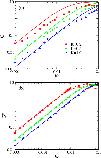
Figure 34: (a) Storage $G^{\prime}$ and (b) loss moduli $G^{\prime\prime}$, as function of oscillation frequency $\omega$ on a double-logarithmic scale, for systems of dumbbells with various spring constants ranging from $K=0.2$ to $K=1.0$. Simulations are performed in two dimensions with the SRD collision rule. The wall separation and the collision time are $L_{y}=10$ and $\Delta t=0.02$, respectively. From Ref. tao_08 .

The behavior of harmonic dumbbells in dilute solution has been studied in detail analytically bird_87_dpl . These results can be used to predict the zero-shear viscosity $\eta$ and the storage and loss moduli, $G^{\prime}(\omega)$ and $G^{\prime\prime}(\omega)$ in oscillatory shear with frequency $\omega$, of the MPC dumbbell fluid. This requires the solvent viscosity and diffusion constant of monomers in the solvent. Since the viscoelastic MPC fluid consists of dumbbells only, the natural assumption is to employ the viscosity $\eta_{MPC}$ and diffusion constant $D$ of an MPC point-particle fluid of the same density. The zero-shear viscosity is then found to be tao_08

$$\eta=\eta_{MPC}\,+\frac{\rho}{2}\,\frac{k_{B}T}{\omega_{H}},$$ (111)

where

$$\omega_{H}=\frac{4K}{\zeta}=\frac{4DK}{k_{B}T}.$$ (112)

Similarly, the storage and loss modulus, and the average dumbbell extension, are predicted to be tao_08

$$G^{\prime} = \frac{\rho k_{B}T}{2}\,\frac{(\omega/\omega_{H})^{2}}{1+(\omega/\omega_{H})^{2}},$$ (113)

$$G^{\prime\prime} = \eta_{MPC}\,\omega+\frac{\rho k_{B}T}{2}\,\frac{\omega/\omega_{H}}{1+(\omega/\omega_{H})^{2}},$$ (114)

and

$$\frac{\langle r^{2}\rangle}{\langle r^{2}\rangle_{\rm eq}}=1+\frac{2}{3}(\dot{\gamma}/\omega_{H})^{2}.$$ (115)

Simulation data are shown in Fig. 34, together with the theoretical predications (113) and (114). The comparison shows a very good agreement. This includes not only the linear and quadratic frequency dependence of $G^{\prime\prime}$ and $G^{\prime}$ for small $\omega$, respectively, but also the leveling off when $\omega$ reaches $\omega_{H}$. In case of $G^{\prime\prime}$, there is quantitative agreement without any adjustable parameters, whereas $G^{\prime}$ is somewhat overestimated by Eq. (113) for small spring constants $K$. The good agreement of theory and simulations implies that the characteristic frequency decreases linearly with decreasing spring constant $K$ and mean free path $\lambda$ (since $D\sim\lambda$). A comparison of other quantities, such as the zero-shear viscosity, shows a similar quantitative agreement tao_08 .

13 Conclusions and Outlook

In the short time since Malevanets and Kapral introduced multi-particle collision (MPC) dynamics as a particle-based mesoscale simulation technique for studying the hydrodynamics of complex fluids, there has been enormous progress. It has been shown that kinetic theory can be generalized to calculate transport coefficients, several collision algorithms have been proposed and employed, and the method has been generalized to describe multi-phase flows and viscoelastic fluids. The primary applications to date—which include studies of the equilibrium dynamics and flow properties of colloids, polymers, and vesicles in solution—have dealt with mesoscopic particles embedded in a single-component Newtonian solvent. An important advantage of this algorithm is that it is very straightforward to model the dynamics for the embedded particles using a hybrid MPC-molecular dynamics simulations approach. The results of these studies are in excellent quantitative agreement with both theoretical predictions and results obtained using other simulation techniques.

How will the method develop in the future? This is of course difficult to predict. However, it seems clear that there will be two main directions, a further development of the method itself, and its application to new problems in Soft Matter hydrodynamics. On the methodological front, there are several very recent developments, like angular-momentum conservation, multi-phase flows and viscoelastic fluids, which have to be explored in more detail. It will also be interesting to combine them to study, e.g., multi-phase flows of viscoelastic fluids. On the application side, the trend will undoubtedly be towards more complex systems, in which thermal fluctuations are important. In such systems, the method can play out its strengths, because the interactions of colloids, polymers, and membranes with the mesoscale solvent can all be treated on the same basis.

- (1) P. J. Hoogerbrugge and J. M. V. A. Koelman, Europhys. Lett. 19, 155 (1992).
- (2) P. Espanol, Phys. Rev. E 52, 1734 (1995).
- (3) P. Espanol and P. B. Warren, Europhys. Lett. 30, 191 (1995).
- (4) G. R. McNamara and G. Zanetti, Phys. Rev. Lett. 61, 2332 (1988).
- (5) X. Shan and H. Chen, Phys. Rev. E 47, 1815 (1993).
- (6) X. He and L.-S. Luo, Phys. Rev. E 56, 6811 (1997).
- (7) G. A. Bird, Molecular Gas Dynamics and the Direct Simulation of Gas Flows (Oxford University Press, Oxford, 1994).
- (8) F. J. Alexander and A. L. Garcia, Comp. in Phys. 11, 588 (1997).
- (9) A. L. Garcia, Numerical Methods for Physics (Prentice Hall, 2000).
- (10) U. Frisch, B. Hasslacher, and Y. Pomeau, Phys. Rev. Lett. 56, 1505 (1986).
- (11) R. Adhikari, K. Stratford, M. E. Cates, and A. J. Wagner, Europhys. Lett. 71, 473 (2005).
- (12) J. K. G. Dhont, An Introduction to Dynamics of Colloids (Elsevier, Amsterdam, 1996).
- (13) R. G. Larson, The Structure and Rheology of Complex Fluids (Oxford University Press, Oxford, 1999).
- (14) M. Ripoll, K. Mussawisade, R. G. Winkler, and G. Gompper, Europhys. Lett. 68, 106 (2004).
- (15) M. Ripoll, K. Mussawisade, R. G. Winkler, and G. Gompper, Phys. Rev. E 72, 016701 (2005).
- (16) M. Hecht, J. Harting, T. Ihle, and H. J. Herrmann, Phys. Rev. E 72, 011408 (2005).
- (17) J. T. Padding and A. A. Louis, Phys. Rev. E 74, 031402 (2006).
- (18) A. Malevanets and R. Kapral, J. Chem. Phys. 110, 8605 (1999).
- (19) A. Malevanets and R. Kapral, J. Chem. Phys. 112, 7260 (2000).
- (20) T. Ihle and D. M. Kroll, Phys. Rev. E 67, 066705 (2003).
- (21) T. Ihle and D. M. Kroll, Phys. Rev. E 63, 020201(R) (2001).
- (22) A. Mohan and P. S. Doyle, Macromolecules 40, 4301 (2007).
- (23) J. M. Kim and P. S. Doyle, J. Chem. Phys. 125, 074906 (2006).
- (24) N. Kikuchi, A. Gent, and J. M. Yeomans, Eur. Phys. J. E 9, 63 (2002).
- (25) M. Ripoll, R. G. Winkler, and G. Gompper, Eur. Phys. J. E 23, 349 (2007).
- (26) N. Kikuchi, C. M. Pooley, J. F. Ryder, and J. M. Yeomans, J. Chem. Phys. 119, 6388 (2003).
- (27) T. Ihle and D. M. Kroll, Phys. Rev. E 67, 066706 (2003).
- (28) T. Ihle, E. Tüzel, and D. M. Kroll, Phys. Rev. E 72, 046707 (2005).
- (29) J. A. Backer, C. P. Lowe, H. C. J. Hoefsloot, and P. D. Iedema, J. Chem. Phys. 122, 1 (2005).
- (30) R. Kapral, Adv. Chem. Phys., to appear (2008).
- (31) E. Allahyarov and G. Gompper, Phys. Rev. E 66, 036702 (2002).
- (32) N. Noguchi, N. Kikuchi, and G. Gompper, Europhys. Lett. 78, 10005 (2007).
- (33) T. Ihle, E. Tüzel, and D. M. Kroll, Europhys. Lett. 73, 664 (2006).
- (34) E. Tüzel, T. Ihle, and D. M. Kroll, Math. Comput. Simulat. 72, 232 (2006).
- (35) C. M. Pooley and J. M. Yeomans, J. Phys. Chem. B 109, 6505 (2005).
- (36) A. Lamura, G. Gompper, T. Ihle, and D. M. Kroll, Europhys. Lett. 56, 319 (2001).
- (37) H. Noguchi and G. Gompper, Phys. Rev. Lett. 93, 258102 (2004).
- (38) I. O. Götze, H. Noguchi, and G. Gompper, Phys. Rev. E 76, 046705 (2007).
- (39) J. F. Ryder, Mesoscopic Simulations of Complex Fluids, Ph.D. thesis, University of Oxford (2005).
- (40) I. O. Götze, private communication (2007).
- (41) J. Erpenbeck, Phys. Rev. Lett. 52, 1333 (1984).
- (42) M. P. Allen and D. J. Tildesley, Computer Simulation of Liquids (Clarendon Press, Oxford, 1987).
- (43) J. H. Irving and J. G. Kirkwood, J. Chem. Phys. 18, 817 (1950).
- (44) H. T. Davis, Statistical Mechanics of Phases, Interfaces, and Thin Films (VCH Publishers, Inc., 1996).
- (45) E. Tüzel, G. Pan, T. Ihle, and D. M. Kroll, Europhys. Lett. 80, 40010 (2007).
- (46) F. Reif, Fundamentals of Statistical and Thermal Thysics (Mc-Graw Hill, 1965).
- (47) R. Zwanzig, Lectures in Theoretical Physics, vol. 3 (Wiley, New York, 1961).
- (48) H. Mori, Prog. Theor. Phys. 33, 423 (1965).
- (49) H. Mori, Prog. Theor. Phys. 34, 399 (1965).
- (50) J. W. Dufty and M. H. Ernst, J. Phys. Chem. 93, 7015 (1989).
- (51) T. Ihle, E. Tüzel, and D. M. Kroll, Phys. Rev. E 70, 035701(R) (2004).
- (52) C. M. Pooley, Mesoscopic Modelling Techniques for Complex Fluids, Ph.D. thesis, University of Oxford (2003).
- (53) E. Tüzel, M. Strauss, T. Ihle, and D. M. Kroll, Phys. Rev. E 68, 036701 (2003).
- (54) E. Tüzel, Particle-bases mesoscale modeling of flow and transport in complex fluids, Ph.D. thesis, University of Minnesota (2006).
- (55) T. Ihle and E. Tüzel, Static and dynamic properties of a particle-based algorithm for non-ideal fluids and binary mixtures (2006), cond-mat/0610350.
- (56) B. J. Berne and R. Pecora, Dynamic Light Scattering: With Applications to Chemistry, Biology and Physics (Wiley, New York, 1976).
- (57) E. Tüzel, T. Ihle, and D. M. Kroll, Phys. Rev. E 74, 056702 (2006).
- (58) H. Noguchi and G. Gompper, Europhys. Lett. 79, 36002 (2007).
- (59) H. Noguchi and G. Gompper, Phys. Rev. E 78, 016706 (2008).
- (60) T. Ihle, submitted to J. Phys.: Condens. Matter (2008).
- (61) H. B. Callen, Thermodynamics (Wiley, New York, 1960).
- (62) Y. Hashimoto, Y. Chen, and H. Ohashi, Comp. Phys. Commun. 129, 56 (2000).
- (63) Y. Inoue, Y. Chen, and H. Ohashi, Comp. Phys. Commun. 201, 191 (2004).
- (64) Y. Inoue, S. Takagi, and Y. Matsumoto, Comp. Fluids 35, 971 (2006).
- (65) T. Sakai, Y. Chen, and H. Ohashi, Comp. Phys. Commun. 129, 75 (2000).
- (66) T. Sakai, Y. Chen, and H. Ohashi, Phys. Rev. E 65, 031503 (2002).
- (67) T. Sakai, Y. Chen, and H. Ohashi, Colloids Surf., A 201, 297 (2002).
- (68) A. Malevanets and J. M. Yeomans, Europhys. Lett. 52, 231 (2000).
- (69) J. Elgeti and G. Gompper, in NIC Symposium 2008, edited by G. Münster, D. Wolf, and M. Kremer (Neumann Institute for Computing, Jülich, 2008), vol. 39 of NIC series, pp. 53–61.
- (70) M. Doi and S. F. Edwards, The Theory of Polymer Dynamics (Oxford University Press, Oxford, 1986).
- (71) E. Falck, O. Punkkinen, I. Vattulainen, and T. Ala-Nissila, Phys. Rev. E 68, 050102(R) (2003).
- (72) R. G. Winkler, K. Mussawisade, M. Ripoll, and G. Gompper, J. Phys.: Condens. Matter 16, S3941 (2004).
- (73) K. Mussawisade, M. Ripoll, R. G. Winkler, and G. Gompper, J. Chem. Phys. 123, 144905 (2005).
- (74) M. A. Webster and J. M. Yeomans, J. Chem. Phys. 122, 164903 (2005).
- (75) E. Falck, J. M. Lahtinen, I. Vattulainen, and T. Ala-Nissila, Eur. Phys. J. E 13, 267 (2004).
- (76) M. Hecht, J. Harting, and H. J. Herrmann, Phys. Rev. E 75, 051404 (2007).
- (77) S. H. Lee and R. Kapral, J. Chem. Phys. 121, 11163 (2004).
- (78) Y. Inoue, Y. Chen, and H. Ohashi, J. Stat. Phys. 107, 85 (2002).
- (79) J. T. Padding, A. Wysocki, H. Löwen, and A. A. Louis, J. Phys.: Condens. Matter 17, S3393 (2005).
- (80) S. H. Lee and R. Kapral, Physica A 298, 56 (2001).
- (81) A. Lamura and G. Gompper, Eur. Phys. J. E 9, 477 (2002).
- (82) J. T. Padding, private communication (2007).
- (83) C. Pierleoni and J.-P. Ryckaert, Phys. Rev. Lett. 61, 2992 (1991).
- (84) B. Dünweg and K. Kremer, Phys. Rev. Lett. 66, 2996 (1991).
- (85) C. Pierleoni and J.-P. Ryckaert, J. Chem. Phys. 96, 8539 (1992).
- (86) B. Dünweg and K. Kremer, J. Chem. Phys. 99, 6983 (1993).
- (87) C. Aust, M. Kröger, and S. Hess, Macromolecules 32, 5660 (1999).
- (88) E. S. Boek, P. V. Coveney, H. N. W. Lekkerkerker, and P. van der Schoot, Phys. Rev. E 55, 3124 (1997).
- (89) P. Ahlrichs and B. Dünweg, Int. J. Mod. Phys. C 9, 1429 (1998).
- (90) P. Ahlrichs, R. Everaers, and B. Dünweg, Phys. Rev. E 64, 040501 (2001).
- (91) N. A. Spenley, Europhys. Lett. 49, 534 (2000).
- (92) C. P. Lowe, A. F. Bakker, and M. W. Dreischor, Europhys. Lett. 67, 397 (2004).
- (93) G. K. Batchelor, J. Fluid Mech. 52, 245 (1972).
- (94) A. J. C. Ladd, Phys. Fluids 9, 481 (1997).
- (95) K. Höfler and S. Schwarzer, Phys. Rev. E 61, 7146 (2000).
- (96) J. T. Padding and A. A. Louis, Phys. Rev. Lett. 93, 220601 (2004).
- (97) H. Hayakawa and K. Ichiki, Phys. Rev. E 51, R3815 (1995).
- (98) H. Hayakawa and K. Ichiki, Phys. Fluids 9, 481 (1997).
- (99) M. H. Ernst, E. H. Hauge, and J. M. J. van Leeuwen, Phys. Rev. Lett. 25, 1254 (1970).
- (100) M. Hecht, J. Harting, M. Bier, J. Reinshagen, and H. J. Herrmann, Phys. Rev. E 74, 021403 (2006).
- (101) B. V. Derjaguin and D. P. Landau, Acta Phys. Chim. 14, 633 (1941).
- (102) W. B. Russel, D. A. Saville, and W. Schowalter, Colloidal dispersions (Cambridge University Press, Cambridge, 1995).
- (103) S. H. Lee and R. Kapral, J. Chem. Phys. 122, 214916 (2005).
- (104) J. G. Kirkwood and J. Riseman, J. Chem. Phys. 16, 565 (1948).
- (105) J. P. Erpenbeck and J. G. Kirkwood, J. Chem. Phys. 29, 909 (1958).
- (106) E. P. Petrov, T. Ohrt, R. G. Winkler, and P. Schwille, Phys. Rev. Lett. 97, 258101 (2006).
- (107) B. H. Zimm, J. Chem. Phys. 24, 269 (1956).
- (108) S. H. Lee and R. Kapral, J. Chem. Phys 124, 214901 (2006).
- (109) M. H. Ernst, E. H. Hauge, and J. M. J. van Leeuwen, Phys. Rev. A 4, 2055 (1971).
- (110) J.-P. Hansen and I. R. McDonald, Theory of Simple Liquids (Academic Press, London, 1986).
- (111) B. Liu and B. Dünweg, J. Chem. Phys. 118, 8061 (2003).
- (112) P. Ahlrichs and B. Dünweg, J. Chem. Phys. 111, 8225 (1999).
- (113) M. Fixmann, J. Chem. Phys. 78, 1594 (1983).
- (114) M. Schmidt and W. Burchard, Macromolecules 14, 210 (1981).
- (115) W. H. Stockmayer and B. Hammouda, Pure & Appl. Chem. 56, 1373 (1984).
- (116) P. E. Rouse, J. Chem. Phys. 21, 1272 (1953).
- (117) P. G. de Gennes, Scaling Concepts in Polymer Physics (Cornell University, Ithaca, 1979).
- (118) J. des Cloizeaux and G. Jannink, Polymer Solutions: Their Modelling and Structure (Clarendon Press, Oxford, 1990).
- (119) D. Ceperly, M. H. Kalos, and J. L. Lebowitz, Macromolecules 14, 1472 (1981).
- (120) K. Kremer and K. Binder, Comput. Phys. Rep. 7, 261 (1988).
- (121) R. G. Winkler, L. Harnau, and P. Reineker, Macromol. Theory Simul. 6, 1007 (1997).
- (122) R. Chang and A. Yethiraj, J. Chem. Phys. 114, 7688 (2001).
- (123) N. Kikuchi, A. Gent, and J. M. Yeomans, Eur. Phys. J. E 9, 63 (2002).
- (124) N. Kikuchi, J. F. Ryder, C. M. Pooley, and J. M. Yeomans, Phys. Rev. E 71, 061804 (2005).
- (125) I. Ali and J. M. Yeomans, J. Chem. Phys. 123, 234903 (2005).
- (126) I. Ali and J. M. Yeomans, J. Chem. Phys. 121, 8635 (2004).
- (127) I. Ali, D. Marenduzzo, and J. F. D. Yeomans, Phys. Rev. Lett. 96, 208102 (2006).
- (128) N. Watari, M. Makino, N. Kikuchi, R. G. Larson, and M. Doi, J. Chem. Phys. 126, 094902 (2007).
- (129) F. Brochard-Wyart, Europhys. Lett. 23, 105 (1993).
- (130) F. Brochard-Wyart, H. Hervet, and P. Pincus, Europhys. Lett. 26, 511 (1994).
- (131) F. Brochard-Wyart, Europhys. Lett. 30, 210 (1995).
- (132) L. Cannavacciuolo, R. G. Winkler, and G. Gompper, EPL 83, 34007 (2008).
- (133) U. S. Agarwal, A. Dutta, and R. A. Mashelkar, Chem. Eng. Sci. 49, 1693 (1994).
- (134) R. M. Jendrejack, D. C. Schwartz, J. J. de Pablo, and M. D. Graham, J. Chem. Phys. 120, 2513 (2004).
- (135) O. B. Usta, J. E. Butler, and A. J. C. Ladd, Phys. Fluids 18, 031703 (2006).
- (136) R. Khare, M. D. Graham, and J. J. de Pablo, Phys. Rev. Lett. 96, 224505 (2006).
- (137) D. Stein, F. H. J. van der Heyden, W. J. A. Koopmans, and C. Dekker, Proc. Natl. Acad. Sci. USA 103, 15853 (2006).
- (138) O. B. Usta, J. E. Butler, and A. J. C. Ladd, Phys. Rev. Lett. 98, 098301 (2007).
- (139) G. S. Grest, K. Kremer, and T. A. Witten, Macromolecules 20, 1376 (1987).
- (140) C. N. Likos, Phys. Rep. 348, 267 (2001).
- (141) D. Vlassopoulos, G. Fytas, T. Pakula, and J. Roovers, J. Phys.: Condens. Matter 13, R855 (2001).
- (142) M. Ripoll, R. G. Winkler, and G. Gompper, Phys. Rev. Lett. 96, 188302 (2006).
- (143) G. S. Grest, K. Kremer, S. T. Milner, and T. A. Witten, Macromolecules 22, 1904 (1989).
- (144) D. R. Mikulencak and J. F. Morris, J. Fluid Mech. 520, 215 (2004).
- (145) A. Link and J. Springer, Macromolecules 26, 464 (1993).
- (146) R. E. Teixeira, H. P. Babcock, E. S. G. Shaqfeh, and S. Chu, Macromolecules 38, 581 (2005).
- (147) R. G. Winkler, Phys. Rev. Lett. 97, 128301 (2006).
- (148) P. G. de Gennes, J. Chem. Phys. 60, 5030 (1974).
- (149) P. LeDuc, C. Haber, G. Bao, and D. Wirtz, Nature (London) 399, 564 (1999).
- (150) D. E. Smith, H. P. Babcock, and S. Chu, Science 283, 1724 (1999).
- (151) C. Aust, M. Kröger, and S. Hess, Macromolecules 35, 8621 (2002).
- (152) Y. Navot, Phys. Fluids 10, 1819 (1998).
- (153) R. Goetz and R. Lipowsky, J. Chem. Phys. 108, 7397 (1998).
- (154) R. Goetz, G. Gompper, and R. Lipowsky, Phys. Rev. Lett. 82, 221 (1999).
- (155) W. K. den Otter and W. J. Briels, J. Chem. Phys. 118, 4712 (2003).
- (156) J. C. Shillcock and R. Lipowsky, J. Chem. Phys. 117, 5048 (2002).
- (157) L. Rekvig, B. Hafskjold, and B. Smit, Phys. Rev. Lett. 92, 116101 (2004).
- (158) M. Laradji and P. B. S. Kumar, Phys. Rev. Lett. 93, 198105 (2004).
- (159) V. Ortiz, S. O. Nielsen, D. E. Discher, M. L. Klein, R. Lipowsky, and J. Shillcock, J. Phys. Chem. B 109, 17708 (2005).
- (160) M. Venturoli, M. M. Sperotto, M. Kranenburg, and B. Smit, Phys. Rep. 437, 1 (2006).
- (161) H. Noguchi and M. Takasu, J. Chem. Phys. 115, 9547 (2001).
- (162) H. Noguchi, J. Chem. Phys. 117, 8130 (2002).
- (163) O. Farago, J. Chem. Phys. 119, 596 (2003).
- (164) I. R. Cooke, K. Kremer, and M. Deserno, Phys. Rev. E 72, 011506 (2005).
- (165) W. Helfrich, Z. Naturforsch. 28c, 693 (1973).
- (166) G. Gompper and D. M. Kroll, J. Phys.: Condens. Matter 9, 8795 (1997).
- (167) G. Gompper and D. M. Kroll, in Statistical Mechanics of Membranes and Surfaces, edited by D. R. Nelson, T. Piran, and S. Weinberg (World Scientific, Singapore, 2004), pp. 359–426, 2nd ed.
- (168) J. M. Drouffe, A. C. Maggs, and S. Leibler, Science 254, 1353 (1991).
- (169) H. Noguchi and G. Gompper, Phys. Rev. E 73, 021903 (2006).
- (170) J.-S. Ho and A. Baumgärtner, Europhys. Lett. 12, 295 (1990).
- (171) D. M. Kroll and G. Gompper, Science 255, 968 (1992).
- (172) D. H. Boal and M. Rao, Phys. Rev. A 45, R6947 (1992).
- (173) G. Gompper and D. M. Kroll, J. Phys. I France 6, 1305 (1996).
- (174) C. Itzykson, in Proceedings of the GIFT Seminar, Jaca 85, edited by J. Abad, M. Asorey, and A. Cruz (World Scientific, Singapore, 1986), pp. 130–188.
- (175) G. Gompper, in Soft Matter – Complex Materials on Mesoscopic Scales, edited by J. K. G. Dhont, G. Gompper, and D. Richter (Forschungszentrum Jülich, Jülich, 2002), vol. 10 of Matter and Materials.
- (176) U. Seifert, K. Berndl, and R. Lipowsky, Phys. Rev. A 44, 1182 (1991).
- (177) G. Gompper and D. M. Kroll, Phys. Rev. Lett. 73, 2139 (1994).
- (178) G. Gompper and D. M. Kroll, Phys. Rev. E 51, 514 (1995).
- (179) H.-G. Döbereiner, G. Gompper, C. Haluska, D. M. Kroll, P. G. Petrov, and K. A. Riske, Phys. Rev. Lett. 91, 048301 (2003).
- (180) H. Noguchi and G. Gompper, Phys. Rev. E 72, 011901 (2005).
- (181) B. Alberts, A. Johnson, J. Lewis, M. Raff, K. Roberts, and P. Walter, Molecular Biology of the Cell (Garland, New York, 2007), 5th ed.
- (182) N. Mohandas and E. Evans, Annu. Rev. Biophys. Biomol. Struct. 23, 787 (1994).
- (183) L. Scheffer, A. Bitler, E. Ben-Jacob, and F. Korenstein, Eur. Biophys. J. 30, 83 (2001).
- (184) G. Lenormand, S. Hénon, A. Richert, J. Siméon, and F. Gallet, Biophys. J. 81, 43 (2001).
- (185) D. E. Discher, D. H. Boal, and S. K. Boey, Biophys. J. 75, 1584 (1998).
- (186) G. Lim, M. Wortis, and R. Mukhopadhyay, Proc. Natl. Acad. Sci. USA 99, 16766 (2002).
- (187) H. Noguchi and G. Gompper, Proc. Natl. Acad. Sci. USA 102, 14159 (2005).
- (188) H. Noguchi and G. Gompper, J. Chem. Phys. 125, 164908 (2006).
- (189) M. M. Dupin, I. Halliday, C. M. Care, L. Alboul, and L. L. Munn, Phys. Rev. E 75, 066707 (2007).
- (190) K. H. de Haas, C. Blom, D. van den Ende, M. H. G. Duits, and J. Mellema, Phys. Rev. E 56, 7132 (1997).
- (191) V. Kantsler and V. Steinberg, Phys. Rev. Lett. 95, 258101 (2005).
- (192) V. Kantsler and V. Steinberg, Phys. Rev. Lett. 96, 036001 (2006).
- (193) M. A. Mader, V. Vitkova, M. Abkarian, A. Viallat, and T. Podgorski, Eur. Phys. J. E 19, 389 (2006).
- (194) S. R. Keller and R. Skalak, J. Fluid Mech. 120, 27 (1982).
- (195) T. W. Secomb and R. Skalak, Q. J. Mech. Appl. Math. 35, 233 (1982).
- (196) T. W. Secomb, T. M. Fischer, and R. Skalak, Biorheology 20, 283 (1983).
- (197) R. Tran-Son-Tay, S. P. Sutera, and P. R. Rao, Biophys. J. 46, 65 (1984).
- (198) U. Seifert, Eur. Phys. J. B 8, 405 (1999).
- (199) C. Misbah, Phys. Rev. Lett. 96, 028104 (2006).
- (200) G. Danker, T. Biben, T. Podgorski, C. Verdier, and C. Misbah, Phys. Rev. E 76, 041905 (2007).
- (201) V. V. Lebedev, K. S. Turitsyn, and S. S. Vergeles, Phys. Rev. Lett. 99, 218101 (2007).
- (202) M. Kraus, W. Wintz, U. Seifert, and R. Lipowsky, Phys. Rev. Lett. 77, 3685 (1996).
- (203) J. Beaucourt, F. Rioual, T. Séon, T. Biben, and C. Misbah, Phys. Rev. E 69, 011906 (2004).
- (204) T. Biben, K. Kassner, and C. Misbah, Phys. Rev. E 72, 041921 (2005).
- (205) H. Noguchi and G. Gompper, Phys. Rev. Lett. 98, 128103 (2007).
- (206) F. Brochard and J. F. Lennon, J. Phys. France 36, 1035 (1975).
- (207) J. Rudnick and G. Gaspari, J. Phys. A 19, L191 (1986).
- (208) G. B. Nash and H. J. Meiselman, Biophys. J. 43, 63 (1983).
- (209) K. Tsukada, E. Sekizuka, C. Oshio, and H. Minamitani, Microvasc. Res. 61, 231 (2001).
- (210) B. M. Discher, Y.-Y. Won, D. S. Ege, J. C.-M. Lee, F. S. Bates, D. E. Discher, and D. A. Hammer, Science 284, 1143 (1999).
- (211) R. Dimova, U. Seifert, B. Pouligny, S. Förster, and H.-G. Döbereiner, Eur. Phys. J. E 7, 241 (2002).
- (212) H. Noguchi and G. Gompper, J. Phys.: Condens. Matter 17, S3439 (2005).
- (213) R. Finken, A. Lamura, U. Seifert, and G. Gompper, Eur. Phys. J. E 25, 309 (2008).
- (214) T. W. Secomb, R. Skalak, N. Özkaya, and J. F. Gross, J. Fluid Mech. 163, 405 (1986).
- (215) R. Skalak, Biorheology 27, 277 (1990).
- (216) R. Bruinsma, Physica A 234, 249 (1996).
- (217) C. Quéguiner and D. Barthès-Biesel, J. Fluid Mech. 348, 349 (1997).
- (218) C. Pozrikidis, Phys. Fluids 17, 031503 (2005).
- (219) C. Pozrikidis, Ann. Biomed. Eng. 33, 165 (2005).
- (220) R. Skalak, Science 164, 717 (1969).
- (221) S. Chien, Ann. Rev. Physiol. 49, 177 (1987).
- (222) Y. Suzuki, N. Tateishi, M. Soutani, and N. Maeda, Microcirc. 3, 49 (1996).
- (223) K. Boryczko, W. Dzwinel, and D. A. Yuen, J. Mol. Modeling 9, 16 (2003).
- (224) W. Dzwinel, K. Boryczko, and D. A. Yuen, J. Colloid Int. Sci. 258, 163 (2003).
- (225) C. D. Eggleton and A. S. Popel, Phys. Fluids 10, 1834 (1998).
- (226) Y. Liu and W. K. Liu, J. Comput. Phys. 220, 139 (2006).
- (227) H. Tanaka, J. Phys.: Condens. Matter 12, R207 (2000).
- (228) J. Vermant and M. J. Solomon, J. Phys.: Condens. Matter 17, R187 (2005).
- (229) Y.-G. Tao, I. O. Götze, and G. Gompper, J. Chem. Phys. 128, 144902 (2008).
- (230) R. B. Bird, C. F. Curtis, R. C. Armstrong, and O. Hassager, Dynamics of Polymeric Liquids, vol. Volume 2: Kinetic Theory (Wiley, New York, 1987).